Fuel Poverty and Health: a Panel Data Analysis

Romanic Baudu, Dorothée Charlier,

Bérangère Legendre

WP 2020.04

Suggested citation: R. Baudu, D. Charlier, B. Legendre (2020). Fuel Poverty and Health: a Panel Data Analysis. FAERE Working Paper, 2020.04.

ISSN number: 2274-5556

www.faere.fr

1

Fuel Poverty and Health: a Panel Data Analysis

Romanic Baudu1, Dorothée Charlier2 and Bérangère Legendre3

December 2019

Protecting and improving health and mitigation of climate change have a shared agenda. In

this paper, we contribute to the literature by assessing the link between fuel poverty and health

over a lengthy recent period. Using dynamic probit models, we examine the influence of fuel

poverty on health. We control for state dependency of health as we regard health status to be

closely related to previous health trajectories. Considering that unobserved heterogeneity

might influence health status and fuel poverty simultaneously, we have corrected for the

endogeneity bias that could affect our results. We conclude that being fuel-poor increases the

risk of bad health by slightly more than a factor of 7 for those whose health is already poor and

by 1.82 for those in good health. For policy makers, combatting fuel poverty reduces sources

of discomfort which might also severely affect the health of a dwelling’s inhabitants.

Keywords: Fuel poverty; Health; Dynamic Probit; Panel dataset

JEL codes: C33; I14; Q41

1/ Introduction

Protecting and improving health and mitigation of climate change have a shared agenda. Public

policies intended to respond to climate change can help reduce health problems. Various

policies can reduce greenhouse gas emissions and produce important health co-benefits (Zivin

& Neidell, 2013) notably through retrofitting of housing (WHO Regional Office for Europe,

1 Université Savoie Mont-Blanc. IREGE. 4 chemin de Bellevue. 74940 Annecy le vieux, FRANCE. 2 Université Savoie Mont-Blanc. IREGE. 4 chemin de Bellevue. 74940 Annecy le vieux, FRANCE. 3 Université Savoie Mont-Blanc. IREGE. 4 chemin de Bellevue. 74940 Annecy le vieux, FRANCE.

2

2004). In northern countries, many households live in homes that have poor thermal conditions

and are therefore expensive to heat, accounting for a substantial share of emissions which in

turn contribute to climate change. Inadequate thermal performance and ventilation of existing

buildings are two of the biggest challenges for the European housing sector with respect to the

sustainability and health of the built environment. Moreover, recent research has demonstrated

that it is possible to improve indoor environmental quality, health and well-being of building

occupants along with improved energy efficiency (Pampuri, Caputo, & Valsangiacomo, 2018;

Prasauskas et al., 2016; Rashid & Zimring, 2008; Stabile, Buonanno, Frattolillo, & Dell’Isola,

2019).

Low-income households may have difficulty paying for energy due to the poor thermal

conditions of the buildings they occupy combined with rising energy prices, and therefore

restrict their energy consumption. These households are considered to be fuel-poor (Boardman,

1991, 2010; Hills, 2011, 2012) and are subject to increased health problems due to the inferior

energy performance of the buildings they live in. Thus, in this paper we contribute to the

literature exploring the impact of being fuel poor on health. The literature on the relationship

between fuel poverty and health is quite limited, while research into the determinants of health

is extensive.

Indeed, the economic and epidemiologic literature on the nexus between air pollution and health

is vast (Contoyannis & Jones, 2004; Neidell, 2004). Local air quality exposure is a significant

driver of health problems (Currie, Neidell, & Schmieder, 2009; Jans, Johansson, & Nilsson,

2018). By reducing air pollution levels, countries can reduce the burden of disease from stroke,

heart disease, lung cancer, and both chronic and acute respiratory diseases, including asthma

(WHO, 2013, 2018). The relationship between socioeconomic characteristics and health is

well-established. . Negative health behaviors and psychosocial characteristics are clustered in

low socioeconomic status groups (Lynch, Kaplan, & Salonen, 1997). The notion that low

socioeconomic status, mainly due to low income, causes poor health is widely supported by

empirical research (Contoyannis, Jones, & Rice, 2004): poverty is associated with poor health

even in advanced industrial societies (Benzeval & Judge, 2001). Education has been also found

to have a positive association with physical and mental health (the so-called education-health

gradient) because individuals invest in their health more effectively and allocate their resources

better (Cutler & Lleras-Muney, 2006). Older people are often in poor health also (Ohrnberger,

Fichera, & Sutton, 2017). While many studies have focused on the drivers of health, they have

3

largely neglected to evaluate the magnitude of fuel poverty on health. Assessing the impact of

fuel poverty on health is necessary for the development of health-related housing policies.

Highlighting this impact would point to the need for coordinated policies. Indeed, housing

improvement policies and energy performance are costly, but these costs should also be

compared with the gains, particularly in terms of health savings.

Additionally, a better understanding of the profile of households in poor health can help policy

makers prevent other households from falling into this state and reduce future health

expenditures. In this context, our objective is to contribute to the literature by assessing the link

between fuel poverty and health over a lengthy recent period (2008-2016). Identifying a precise,

direct and mid-term link between fuel poverty and health seems crucial in the design of relevant

public policies. Implementing an effective policy implies anticipating both intermediate and

final objectives: tackling fuel poverty as the intermediate objective and improving public health

as the final objective. Thus, we use panel data (EU-SILC) to consider individual health and

household fuel poverty trajectories, but also to avoid obtaining results affected by 1-year

climate variables. We focus on the French situation where the direct medical cost related to

poor housing is estimated to be 930 million euros (Eurofound, 2016). The indirect annual costs

are estimated to be 20.3 billion euros. Using dynamic probit models, we tested the influence of

fuel poverty on health. We controlled for state dependency of health as we consider health status

to be closely related to health status in the previous year. We also controlled for initial

conditions (Heckman, 1981). Considering that unobserved heterogeneity might have an impact

on health status and fuel poverty simultaneously, we corrected for the endogeneity bias that

could affect our results. In order to improve the living conditions of households in fuel poverty,

both short- and long-term policies are needed. Supplementing the household income and

reducing energy costs will help in the short term, but improving the energy efficiency of housing

(e.g. modernizing heating systems, installing thermal insulation) is the long-term solution to

address fuel poverty and its health consequences. Energy-efficient housing not only has benefits

for the health of occupants, but also for society as a whole.

The next section presents the existing literature on the relationship between energy efficiency

and health. The theoretical background is then introduced. Data are presented in the fourth

section, and the empirical strategy is introduced in the fifth section. The results are presented

in Section 6, along with a key policy recommendation. We conclude in Section 7.

4

2. Methods

2.1 Literature on energy efficiency and health

The literature extensively documents the impact of cold, damp housing and mold on health

(Maidment, Jones, Webb, Hathway, & Gilbertson, 2014; Peat, Dickerson, & Li, 1998; Platt,

Martin, Hunt, & Lewis, 1989). There is much evidence that poor housing conditions, combined

with financial constraints may worsen both mental and physical health (Hills, 2012; Hunt, 1988;

Maidment et al., 2014; Platt et al., 1989; University College, Team, & Earth, 2011). Persistently

low temperatures in housing lead to respiratory tract infections and coronary problems,

increased blood pressure, worsening arthritis, along with more frequent accidents in the home

and adverse effects on children’s education and nutrition (National Heart Forum, 2003).

Dampness and mold that accumulate in cold homes increase respiratory symptoms including

asthma, coughing and wheezing (Dales, Zwanenburg, Burnett, & Franklin, 1991; Jaakkola,

Hwang, & Jaakkola, 2005; Peat et al., 1998). In their meta-analysis Fisk, Lei-Gomez, and

Mendell (2007) conclude that dampness and mold are associated with increases of 30–50% in

respiratory and asthma-related health problems. Cold and damp housing may also affect well-

being and cause stress and depression in its inhabitants (Khanom, 2000; Lowry, 1991; Shortt

& Rugkåsa, 2007). Poor-quality housing can expose households to cancer risks , due to

exposure to radon, or to formaldehyde from combustion or off-gassing (Braubach, Jacobs, &

Ormandy, 2011).

Thus, improving energy efficiency reduces health problems. In an experiment conducted in

south Devon in the UK, Barton et al. (2007) concluded that improving heating and insulation

reduces chest problems and asthma symptoms, at least in the short term. After conducting a

fuel poverty program in 54 rural homes in Ireland, Shortt and Rugkåsa (2007) showed that the

installation of central heating systems and development of energy-efficiency awareness led to

a significant decrease in both the numbers of householders reporting arthritis/rheumatism and

other forms of illness. A pilot study in Cornwall established that installation of central heating

was an effective measure for reducing nocturnal cough and asthma in children, and

consequently time lost from school (Sorrell, Dimitropoulos, & Sommerville, 2009). Other

5

studies have demonstrated the general impact of fuel poverty on health (Liddell & Morris,

2010).

Public policies such as retrofitting and saving energy pursue an intermediate objective which is

the reduction of fuel poverty, but also have an impact on public health as a final objective. For

households, retrofitting increases comfort, as housing conditions are improved. The quality of

the dwelling might be improved through heating upgrades (Chapman, Howden-Chapman,

Viggers, O'Dea, & Kennedy, 2009), better insulation (Bourdon, Van Mien, & Normand-Cyrot,

1992; Homøe, Christensen, & Bretlau, 1999; Vandentorren et al., 2006), draftproofing/sealing

around doors or windows (P. Howden-Chapman et al., 2005; Philippa Howden-Chapman,

Phipps, & Cunningham, 2007), glazing improvements (Iversen, Bach, & Lundqvist, 1986) or a

combination of different measures (Lloyd, Callau, Bishop, & Smith, 2008).

The literature includes many case studies which were carried out with experimental data. Some

of them explore the direct impact of retrofitting plans, housing improvements and/or energy-

saving programs on health4 (Chapman et al., 2009; Philippa Howden-Chapman et al., 2007;

Lloyd et al., 2008) (Chapman et al., 2009; Ezratty, Duburcq, Emery, & Lambrozo, 2009;

Thomson & Snell, 2013). Others do not measure the impact on health but assess domestic

energy use after retrofitting in order to estimate the likely health impact of an intervention from

an intermediate outcome, such as temperature or air quality and carbon emissions (Rosenow &

Galvin, 2013). Some studies evaluate the actual impact of energy consumption and fuel poverty

(Rosenow & Galvin, 2013) (Grimes et al., 2016; Webber, Gouldson, & Kerr, 2015).

Case studies and experiments make it possible to precisely evaluate the impact of policies on a

given region at a particular point in time, thus providing useful guidance for designing or

improving public policy. However, they fail to establish a clear causal relationship between fuel

poverty and health in the absence of any retrofitting, energy-saving measures or housing

improvements. When non-experimental studies confirm a link between fuel poverty and health

(Chaton & Lacroix, 2018; Lacroix & Chaton, 2015; Liddell & Morris, 2010), the results are

based on cross-sectional data, ignoring the effects of health trajectories and climate hazards on

4 See Maidment et al. (2014) for a meta-analysis including 36 studies which evaluate the relationship between household energy-efficiency interventions and the health of the occupants

6

fuel poverty. The effects of climate hazards are then determined by conducting an evaluation

ex-ante, and/or ex-post and by carrying out a non-experimental study.

2.3 Data

In this study, we wish to shed light on the potential causal effect of energy precariousness on

the health of individuals. Thus, econometric analysis was conducted using the French portion

of the EU-SILC5 database (European Union – Community Statistics on Income and Living

Conditions). We chose data from 2008 until 2016, which is the last survey to date. This time

frame was selected since the year 2008 marked significant changes, such as improving the

accuracy of household resources using data from public institutions, and specifying the type of

energy used inside dwellings instead of a global indicator, which is fundamental to the

construction of relevant fuel poverty indicators (Hills, 2011, 2012). The database also includes

some health indicators, such as self-assessed health condition, the presence of chronic diseases

and handicaps, potentially unfulfilled needs to see a specialist and the reasons for this, and other

health-related variables, thus providing a good set of tools for describing and controlling the

effect of fuel poverty on health. The database also contains many variables characterizing socio-

economic status, demographic status and living conditions related to housing and energy use of

individuals, thus provides a solid basis for assessing health and fuel poverty under the many

aspects and definitions reviewed in the literature. The entire sample consisted of 239,477

observations over nine years.

Our health indicator is the self-assessed health status of the respondents; this will be our binary

dependent variable, with 1 for poor health. Some 8.3% of individuals declared a status of poor

health over the period studied. While a categorical self-assessed health variable is a wide

measure of one’s mental and physical condition, its reliability could be questionable (Crossley

& Kennedy, 2002). However it remains one of the best tools available to measure health as it

predicts future mortality and morbidity adequately (Idler & Kasl, 1995; Lundberg &

Manderbacka, 1996). We also use a stated binary variable for chronic disease as a control

(robustness check); 37.3% of individuals in the sample report a chronic disease. A chi square

test of independence shows that having a chronic disease is not independent from declaring a

5 The EU-SILC project was established in response to a request from the European Commission and is led by Eurostat. The French part of the project is called SRCV (Statistiques sur les Ressources et Conditions de Vie)

7

status of poor health. Among people who declared a status of poor health, 94% had a chronic

disease. In this study, we are interested in the possible continuity of health status. In our sample,

the 95.9% of individuals who reported a status of good health, reported this over the entire

period. Only 4.1% of individuals saw their health deteriorate, whereas 41% reported a status of

poor health at the beginning of the period and saw their health improve.

To measure fuel poverty, we chose to apply the most common indicators of fuel poverty defined

and used in the literature (which will be our main predictors): the 10% ratio6 (Boardman, 1991)

and Low Income High Costs (LIHC) 7 (Hills, 2011, 2012). Both of these measures are calculated

based on the standard of living8 (SL) of the households observed rather than the disposable

income of the household. The 10% ratio permits comparisons and serves as a reference. We

built it by aggregating electricity, natural gas and other heating expenditures whether or not

included in the rent, and calculating its share of the SL which gives us the energy effort rate of

individuals, and compared it to the 10% threshold, resulting in a binary variable (1=fuel poor,

0=not fuel poor). There is some criticism in the literature about this measure of fuel poverty,

mainly due to the fact that high income individuals who spend a lot on energy can be considered

to be fuel poor while being nowhere near fuel poverty socially speaking (Healy & Clinch,

2002), so we have also compared our results with the LIHC indicator9. We did this by

comparing an individual’s SL to a poverty threshold10 on the one hand and then comparing the

individual’s fuel expenditures to an expenditure threshold11. If one has a SL below the poverty

threshold, and spends more on energy than the expenditure threshold, the individual is then

considered to be fuel poor (1=fuel poor, 0=not fuel poor). In our sample 4.78% are fuel poor

according to the 10% ratio and 5.74% according to the LIHC.

We tested the independence of fuel poverty (10% definition) and health status. The chi square

test allows us to reject the hypothesis of independence between fuel poverty and poor health at

the 1% level. Similar results are obtained if we consider another definition of fuel poverty or

6 Based on the first measure used in the UK, 10% representing the ratio between the double median of heating energy expenditure of the population and their income. If one’s own ratio is over this threshold, then the individual is considered to be fuel poor. 7 The LIHC is used in the analysis to prove the robustness of results obtained later. 8 Disposable income / consumption unit (OECD equivalent scale) 9 Due to the cultural heterogeneity of European countries, as well as EU resistance to acknowledge a pan-European definition of fuel poverty (Thomson et al., 2017), the debate on how to measure it precisely and exhaustively is still raging. Our objective in this paper is not to discuss measurement of fuel poverty, but to determine if fuel-poor individuals have a worse health status that those who are not fuel-poor. 10 This particular threshold is fixed at 60% of the median of income after energy costs by consumption unit. 11 Which is the median fuel expenditure among the observed population.

8

another measure of health i.e. having a chronic disease. Generally speaking, more fuel-poor

households are in poor health (Figure 1).

Figure 1 Health status according to fuel poverty definition

Finally, we introduced variables for controlling for health status: socio-demographic

characteristics and local conditions (weather and pollution).

Degree level and home ownership are especially used as proxies to better control the standard

of living and the wealth of individuals.

Health status might also be linked to climate (WHO, 2013). Our dataset gave us access to

information about the climate zone where each household is located. This was matched with

meteorological data of Meteo France (unified degree days12) to provide a proxy for the actual

meteorological conditions. Finally, we approximated the income variable with level of

education to avoid multicollinearity with fuel poverty (based on income). The descriptive

statistics are presented in Table 1, and all variables are defined in Appendix 1.

12 Unified Degree Days express the severity of cold weather in a specific time period taking into consideration actual outdoor temperature and an average reference temperature previously recorded.

9

Table 1 Descriptive statistics

Variable Mean Std Dev Min Max Observations Poor health overall 0.084 0.277 0.000 1.000 N = 187817 between 0.246 0.000 1.000 n = 53430 within 0.166 -0.805 0.972 Chronic disease overall 0.372 0.483 0.000 1.000 N = 187803 between 0.423 0.000 1.000 n = 53438 within 0.264 -0.516 1.261 Fuel poverty 10% overall 0.048 0.213 0.000 1.000 N = 239477 between 0.178 0.000 1.000 n = 67030 within 0.137 -0.841 0.937 Fuel poverty LIHC overall 0.057 0.233 0.000 1.000 N = 239477 between 0.197 0.000 1.000 n = 67030 within 0.153 -0.832 0.946 Pollution overall 0.121 0.326 0.000 1.000 N = 239477 between 0.273 0.000 1.000 n = 67030 within 0.213 -0.768 1.010 Number of children overall 1.282 1.298 0.000 11.000 N = 239475 between 1.290 0.000 11.000 n = 67030 within 0.297 -2.718 4.949 Age overall 40.507 23.586 0.000 102.000 N = 239475 between 23.840 0.000 101.000 n = 67030 within 1.565 13.507 54.507 Undergraduate degree overall 0.082 0.274 0.000 1.000 N = 239477

between 0.257 0.000 1.000 n = 67030 within 0.099 -0.807 0.971 Homeowner overall 0.676 0.468 0.000 1.000 N = 239477 between 0.463 0.000 1.000 n = 67030 within 0.138 -0.213 1.564 Medical density overall 302.65 39.64 243.70 403.00 N = 239477 between 38.77 243.70 403.00 n = 67030 within 10.50 203.73 392.98 Dark dwelling overall 0.077 0.267 0.000 1.000 N = 239452 between 0.232 0.000 1.000 n = 67026 within 0.166 -0.812 0.966 Electricity price overall 0.162 0.035 0.000 0.200 N = 239477 between 0.028 0.000 0.200 n = 67030 within 0.025 0.007 0.329 Gas price overall 0.051 0.037 0.000 0.130 N = 239477 between 0.033 0.000 0.130 n = 67030 within 0.021 -0.054 0.165 Unified degree days overall 1928 355 1054 2683 N = 219431 between 297 1054 2683 n = 61324 within 214 906 2904

10

2.4 Empirical model

This paper presents an approach based on traditional consumer theory where

representation of individual preferences is based on the bundle of goods they have chosen to

maximize their utility or well-being. Theoretical foundations are presented in appendix

(Appendix 2).

We estimate the impact of fuel poverty on the probability of being in poor health

controlling for other characteristics (based on equation 3, section 2). We use panel probit

models and propose four configurations, first to control for state-dependence of health

(Contoyannis et al., 2004), and second to control for endogeneity of fuel poverty (Awaworyi

Churchill & Smyth, 2018).

So, we have as the first model specification (Model 1):

ℎ ∗#$= 𝛼𝑋#$ + 𝛽𝑊#$ + 𝛾𝐹𝑃#$ + 𝑢# + 𝑣#$ (4)

With:

𝑖 = 1,… ,𝑁𝑎𝑛𝑑𝑡 = 1,… , 𝑇

ℎ#$ = 1if ℎ#$∗ > 0 and 0 otherwise

ℎ#$ represents the health status of the individual 𝑖 in 𝑡, equal to 1 for good health at time t, 𝑋#$

is the vector of observed variables (including age, level of education, etc.), 𝑊#< is a vector of

living conditions including local air pollution and climate, 𝐹𝑃#$ is the fuel poverty regressor,

equal to 1 for a fuel-poor individual, according to the 10% threshold., 𝑢# the individual-specific

effect assumed to be unrelated to control variables, and 𝑣#$ the idiosyncratic error term.

However, health status has a certain degree of persistence over time (Contoyannis et al.,

2004), which leads to the first configuration being biased. To account for this state-dependence

(Carro & Traferri, 2014; Halliday, 2008), we include a lagged health status variable

representing the health of individuals in the previous year.

So, we propose a dynamic random effect model:

11

ℎ#$∗ = 𝛿ℎ#$>? + 𝛼𝑋#$ + 𝛽𝑊#$ + 𝛾𝐹𝑃#$ + 𝑢# + 𝑣#$ (5)

ℎ#$>? representing the lagged health status.

The use of a lagged variable presents the initial conditions problem (Heckman, 1981). The

historic stochastic process of health status is not observed at the beginning. The initial values

of this variable cannot be considered exogenous (Akay, 2009). Health during childhood, or

other exogenous parameters affect the entire health trajectory for example (Contoyannis et al.,

2004; Halliday, 2008). So, we can express health at the first period in the panel as following:

ℎ#@∗ = 𝛾𝑍#@ + 𝜃𝑢# + 𝜀# (6)

With 𝑍#@ including exogenous attributes affecting health status in the first period. The initial

conditions problem leads 𝑦#@ then to be correlated with the unobserved heterogeneity.

Consequently, in equation (2) we have 𝐸(𝑢#|𝑦#@) ≠ 0 when 𝜃 ≠ 0.

In order to treat the initial conditions problem, we use the inverse of Mills’ ratio13 within the

Orme’s two-step method (Arulampalam & Stewart, 2007; Orme, 1997). We estimate a probit

of the probability of being in good health in the first year in the panel. The medical density14

i.e. the ratio of physicians (practitioners or specialists) to the population in a geographic area,

is used as an exogenous instrument (𝑍#@) to explain the health status at time 𝑡@ (Chaix,

Veugelers, Boëlle, & Chauvin, 2005; Macinko, Starfield, & Shi, 2003).

Our second specification, correcting the initial conditions problem, might be expressed as

follows (Model 2):

ℎ#$∗ = 𝛿ℎ#$>? + 𝛼𝑋#$ + 𝛽𝑊#$ + 𝛾𝐹𝑃#$ + 𝜎𝐸[𝑢#|𝑦#@] + 𝑢#∗ + 𝑣#$ (7)

in which 𝐸[𝑢#|𝑦#@]has been estimated in the first step as:

13 Which is a monotone decreasing function of the probability of the selection of an observation in the sample (Heckman, 1979) 14 Data from the French Atlas of Medical Demography14, carried out annually by the French Medical Board,

adjusted by national territory divisions have been used to construct the variable of medical density.

12

𝐸[𝑢#|𝑦#@] = 𝐸[𝑢#|𝜃𝑢# + 𝜀# ≥ −𝛾𝑍#$] = 𝜙(𝛾𝑍#$)Φ(𝛾𝑍#$)

The third specification of the model accounts for the potential endogeneity of fuel

poverty as we cannot rule out that unobserved heterogeneity simultaneously affects health and

fuel poverty (Awaworyi Churchill & Smyth, 2018). We adopt a two-step instrumental method

(Heckman, 1979) by first estimating fuel poverty. Electricity and natural gas prices are used as

instruments as they are the most commonly used sources of energy for heating (Ambrosio,

Belaid, Bair, & Teissier, 2015). Energy prices are often recognized as one of the most important

determinants of residential energy demand (see Labandeira, 2017 Labandeira, Labeaga, and

López-Otero (2017) for a literature review) and as a consequence of energy expenditures, a

main component of fuel poverty (Charlier & Kahouli, 2019; ONPE 2014). We extrapolate the

fuel price rate of each individual using the surface area of their dwelling and their fuel bills. In

order to estimate fuel poverty more precisely, we also introduce a variable to consider energy

efficiency from the solar exposure of the dwelling (Charlier & Kahouli, 2019), a binary variable

if the dwelling is dark.

The predicted value of fuel poverty is thus obtained using equation 8:

𝐹𝑃#$∗ = 𝜃?𝑋#$ + 𝜃R𝑊#$ + 𝜃S𝐺𝑎𝑠_𝑝#$ + 𝜃X𝐸𝑙𝑒𝑐_𝑝#$ + 𝜃\𝐺𝑎𝑠𝐸𝑙𝑒𝑐_𝑝#$ + 𝜃]𝐷#$ + 𝑢#_ + 𝑣#$_

(8)

With 𝑝#$ = 1if 𝑝#$∗ > 0 and 0 otherwise.

𝐺𝑎𝑠_𝑝#$, 𝐸𝑙𝑒𝑐_𝑝#$ are the gas price and the electricity price, 𝐺𝑎𝑠𝐸𝑙𝑒𝑐_𝑝#$ the interaction

parameter between both energy prices to account for potential multicollinearity between

evolution of energy prices15 and 𝐷#$, a dummy variable indicating if the dwelling is dark.

The third specification of the model is a dynamic probit model, with correction of the

endogeneity bias caused by the fuel poverty variable (Model 3):

15 Before 2008, energy prices rose rapidly and fell sharply during the 2009 crisis, which explains why energy expenditures were quite low during this period compared to the previous. However, since 2010, the price of oil increased as did household energy expenditures, reaching a peak in 2013. Then, considering France had recorded several mild winters, the share of energy expenditure in the overall budget continued to grow ((ONPE, 2018))

13

ℎ#$∗ = 𝛿𝑦#$>? + 𝛼𝑋#$ + 𝛽𝑊#$ + 𝛾𝐹𝑃 $a + 𝜎𝐸[𝑢#|𝑦#@] + 𝑢#∗ + 𝑣#$ (5)

Finally, the fourth specification controls the sensitivity to the choice of health variable. We

estimate the third model and replace the health variable with a binary variable for chronic

disease (Model 4). Then, we apply bootstrap techniques in each step to avoid bias (Efron &

Tibshirani, 1993; Horowitz, 2003).

3. Results and discussion

The main results are reported in Table 2. For the sake of clarity, the results of the initial

conditions equation and the endogeneity treatment of fuel poverty equation are reported in the

Appendix (See Appendix 3).

The results of the four models are reported in Table 2, but there is no doubt that only models 3

and 4 contribute to correctly identifying the causal effect of fuel poverty on health. We will

therefore discuss these results directly.

The estimates confirm the negative impact of fuel poverty on health status, as expected in the

theoretical model, and as previously established in different cross-sectional case studies (Table

2, Models 1 to 4).

The impact of fuel poverty appears to be strong (Table 2, Model 3): being fuel poor increases

the risk of bad health by more than a factor of 7 (Table 3, Model 3) for those already in poor

health, and by a factor of 1.82 for those who were in good health in the previous year. Finally,

to test the robustness of the results established by Models 1 to 3, we use an objective measure

of health, the existence of chronic diseases (Model 4). This last model confirms that being fuel

poor multiplies the risk of chronic disease by more than a factor of 6.14 (Table 3, Model 4) for

those in good health (no chronic disease) in the previous year, and by 7.88 for those who already

declared at least one chronic disease. If we account for the unobserved heterogeneity affecting

exposure to fuel poverty and deteriorating health simultaneously, we can conclude there is a

very strong causal relationship between both phenomena.

The empirical strategy adopted first shows that the nature of the health variable has to be

accounted for, and second that neglecting endogeneity of fuel poverty would lead to a

14

significant underestimation of the health risk. The entire health trajectory of each individual has

to be controlled: the intermediate estimate consisting of the control of initial conditions shows

that medical density is a good instrument to explain the health of individuals before their entry

in the panel (Table 6, Appendix 3A). Medical density significantly decreases the probability of

being in poor health and of having a chronic disease.

The effects of path dependency in health are evident in Tables 2 and 3, and confirms the

necessity to control initial conditions: being in poor health in the previous period significantly

increases first the risk of poorer health and secondly the impact of fuel poverty. A self-

perpetuating spiral, reinforced by energy insecurity, is then triggered.

The first step in Models 3 and 4 which provides the estimated fuel poverty probability also

allows us to conclude that energy prices are good instruments and strongly affect exposure to

fuel poverty (Table 7 in Appendix 3B). When electricity and gas prices increase, the risk of fuel

poverty increases significantly for each individual. Having a dark dwelling also significantly

increases the probability of being poor. This step enables us to provide a good prediction of

fuel poverty: the correct prediction rate is about 87%.

To test the robustness of the results established in the Models 3 and 4, we introduced an

alternative indicator of fuel poverty: the low-income high cost indicator. According to this

definition, households are fuel-poor if they have an income after fuel costs that is below the

poverty threshold16 as well as fuel costs above the median population fuel cost. These estimates

are reported in the Appendix (Table 8 in Appendix 3C). We have validated the results and

particularly the size of the effect: being fuel poor leads to an increase in the risk of bad health

by more than a factor of 2 for a person previously in good health and by more than 8 for those

already in poor health (Table 9 model 3). The risk of declaring a chronic disease increases by a

factor of 4.38 for a healthy person (Table 9 Model 4).

16 This poverty threshold is set at 60% of the population income, from which fuel costs have been deducted.

15

Table 2 results - probability of being in poor health

Model 1 Model 2 Model 3 Model 4 To be in poor health

(lag)

1.611*** 1.609***

(0.0328) (0.0328)

Fuel poverty 10% 0.252*** 0.198***

(0.0332) (0.0630)

Number of children 0.0824*** 0.0353*** 0.0188** 0.00461 (0.0127) (0.0118) (0.00857) (0.00607)

Unified Degree Days (log)

0.0527 0.0306 -0.0280 -0.0823***

(0.0466) (0.0361) (0.0371) (0.0252) Age 0.0529*** 0.0216*** 0.00139 -0.000319

(0.00100) (0.00651) (0.00272) (0.00190) Pollution problem 0.186*** 0.142*** 0.0202 0.0708***

(0.0247) (0.0515) (0.0273) (0.0179) Undergraduate degree -0.365*** -0.186*** 0.0287 0.0160

(0.0469) (0.0718) (0.0397) (0.0176) Homeowner -0.642*** -0.281*** -0.0208 0.00102

(0.0274) (0.0915) (0.0392) (0.0158) Mills’ ratio

-0.0219 -0.836*** -0.895*** (0.293) (0.119) (0.0994)

Predicted fuel poverty 10%

21.39*** 25.15***

(3.357) (2.964)

Chronic disease (lag)

1.548*** (0.0210)

Constant -5.568*** -3.068*** -0.242 0.526* (0.362) (0.828) (0.431) (0.286)

Observations 173,88 122,362 122,347 122,32 Number of individuals 49,422 37,855 37,855 37,861

Robust standard errors in parentheses

*** p<0.01, ** p<0.05, * p<0.1

16

Table 3 Marginal effect of fuel poverty (10%) on poor health

Model 1 0.019***

Good health in t-1 Poor health in t-1

Model 2 0.017*** 0.065***

Model 3 1.82*** 7.05***

Model 4 6.14*** 7.88*** *** p<0.01, ** p<0.05, * p<0.1

Finally, using the same methodology, we wanted to identify the threshold where the effort rate

significantly increases the probability of being in poor health . Results for predictive values are

presented in Figure 2 below. We note that from a predicted effort rate of 25%, the probability

of being in poor health is greater than being in good health.

Figure 2: Predictive margins for effort rate – linear prediction

The concept revealed in Figure 2 is confirmed when replaced in Model 3 (the most complete,

the variable of fuel poverty multiplied by the effort rate). The results are reported in Table 4:

17

when the effort rate increases marginally, the risk of declaring a state of poor health increases

by 5.5.

Table 4 Results - probability of being in poor health

Poor health (lag) 1.613*** (0.0329)

Predicted effort rate 5.505*** (1.522)

Number of children 0.0158* (0.00936)

Unified Degree Days (log) -0.0245 (0.0408)

Age 0.00172 (0.00370)

Pollution problem 0.0203 (0.0334)

Undergraduate degree 0.0514 (0.0482)

Homeowner -0.0560 (0.0537)

Mills’ ratio -0.853*** (0.165)

Panel-level variance (log) -1.727*** (0.132)

Constant -0.433 (0.526)

Observations 122,345 Number of individuals 37,855

Robust standard errors in parentheses – Bootstrap 5000 replications

*** p<0.01, ** p<0.05, * p<0.1

Our results reinforce the estimates provided by the National Housing Federation in 2010: the

cost for treating ill health resulting from poor housing conditions has been estimated at GBP

2.5 billion per year in the UK. Eurofound (2016) models the cost of housing inadequacies and

estimated that in France, 930 million euros in medical expenses would be saved by repairing

inadequate housing. The previous reports combined with our results lead us to conclude that

spillover effects exist in public policy: implementing policies which promote energy efficiency,

18

such as encouraging investment in retrofitting are useful tools for tackling fuel poverty and

also reduce medical spending.

Retrofitting policies, in this sense, go beyond the simple monetary benefits: a household could

occupy an energy-inefficient dwelling and cope with it by means of a high income. Retrofitting

measures would still be highly beneficial to them due to improvement of the environment. In

the context of continuous increases in energy prices in Europe as shown by Eurostat (2019),

investment opportunities created by the need for energy efficiency are vast and highly profitable

(Amstalden, Kost, Nathani, & Imboden, 2007). Retrofitting plans and energy efficiency

measures have an impact on fuel poverty through different channels. First, they directly and

robustly improve living conditions (reduce cold, dampness, mold). Second, they lead indirectly

to a decrease in energy costs, particularly because the housing becomes less energy-intensive.

Finally, reducing residential energy consumption/demand reduces carbon dioxide emissions,

which is an important component of the preservation of climate and natural resources, and the

environment as a whole. “For example, cleaner energy systems could reduce carbon emissions,

and cut the burden of household air pollution, which causes some 4.3 million deaths per year,

and ambient air pollution, which causes about 3 million deaths every year” (WHO, 2018).

More broadly, our results beg the question whether it is possible to achieve energy transition

without considering the impact of fuel costs on fuel poverty and the indirect impact on public

health. Achieving energy transition without incurring excessive economic and social costs

requires anticipating long chain reactions.

7/ Conclusion Fuel poverty has been treated extensively in recent literature. But very few studies target the

causal link between fuel poverty and poor health. Numerous papers focus on specific

experiments assessing the link between some timely retrofitting policies and the health of

occupants (Chapman et al., 2009; Ezratty et al., 2009; Philippa Howden-Chapman, 2015;

Philippa Howden-Chapman et al., 2007; Lloyd et al., 2008; Thomson & Snell, 2013). To the

best of our knowledge only two papers (Lacroix & Chaton, 2015; Liddell & Morris, 2010)

describe non-experimental and cross-sectional research on the relationship between fuel

poverty and health. Our study aims to go beyond the limits of this previous work, namely the

19

overly specific aspects of experimental studies and the non-generalizable results of cross-

sectional research that neglect climate hazards and the path dependency of health.

In the present paper, we estimate the causal effect of fuel poverty on health status. To do this,

we used panel data from the EU-SILC over a lengthy recent period (2008-2016) and estimated

probit panel models in four steps. We begin with a simple probit model without controlling for

state dependency of health and endogeneity of fuel poverty, and finish with a dynamic probit

model controlling for both biases.

We conclude that fuel poverty has a significant impact on health. Being fuel poor increases the

risk of bad health by slightly more than a factor of 7 for those already in poor health (1.82 for

those in good health) and by 7.88 the risk of having a chronic disease for those who already

have a chronic disease (6.14 for those previously in good health). In terms of policy

recommendations, we stress the importance of energy-efficiency retrofits. This type of policy

will not only make it possible, to improve the housing conditions of households and their well-

being, but also to reduce their energy bills and thus their exposure to fuel poverty. Indirectly,

our work suggests that such policies could also have a positive impact on health spending.

Lessons learned from our empirical strategy also allow us to conclude that neglecting path

dependency of health and endogeneity of fuel poverty leads to a substantial underestimation of

the impact on health. By controlling both biases, we first show that medical density must be

accounted for to achieve a good understanding of the health history of each individual.

Secondly, as energy prices are good instruments for controlling endogeneity, our results

question the inextricably linked issues of energy transition, combatting fuel poverty and

safeguarding public health. Is it possible to achieve energy transition without excessive

economic and social costs, i.e. without increasing fuel poverty and damaging public health?

Acknowledgment

This work was supported by Auvergne-Rhône-Alpes FRANCE region (Pack Ambition

Recherche)

20

References

Akay, A. (2009). The Wooldridge Method for the Initial Values Problem is Simple: What about Performance? , 42.

Ambrosio, G., Belaid, F., Bair, S., & Teissier, O. (2015). Observatoire de la Precarite Energe tique. 59.

Amstalden, R. W., Kost, M., Nathani, C., & Imboden, D. M. (2007). Economic potential of energy-efficient retrofitting in the Swiss residential building sector: The effects of policy instruments and energy price expectations. Energy Policy, 35(3), 1819-1829. doi:10.1016/j.enpol.2006.05.018

Arulampalam, W., & Stewart, M. B. (2007). Simplified Implementation of the Heckman Estimator of the Dynamic Probit Model and a Comparison with Alternative Estimators.

Awaworyi Churchill, S., & Smyth, R. (2018). Energy Poverty and Health: Panel Data Evidence from Australia.

Barton, A., Basham, M., Foy, C., Buckingham, K., Somerville, M., & Torbay Healthy Housing, G. (2007). The Watcombe Housing Study: the short term effect of improving housing conditions on the health of residents. Journal of epidemiology and community health, 61(9), 771-777. doi:10.1136/jech.2006.048462

Benzeval, M., & Judge, K. (2001). Income and health: the time dimension. Social Science & Medicine, 52(9), 1371-1390. doi:https://doi.org/10.1016/S0277-9536(00)00244-6

Boardman, B. (1991). Fuel Poverty: From Cold Homes to Affordable Warmth. London: Belhaven Press.

Boardman, B. (2010). Fixing Fuel Poverty: Challenges and Solutions. London: Earthscan.

Bourdon, P., Van Mien, H. D., & Normand-Cyrot, D. (1992). Power Plants: Nonlinear Modelling. In D. P. A. Borne (Ed.), Concise Encyclopedia of Modelling & Simulation (pp. 358-363). Oxford: Pergamon.

Braubach, M., Jacobs, D. E., & Ormandy, D. (2011). Environmental burden of disease associated with inadequate housing: a method guide to the quantification of health effects of selected housing riss in the WHO European Region. Copenhagen: World Health Organization, Regional Office for Europe.

Carro, J. M., & Traferri, A. (2014). STATE DEPENDENCE AND HETEROGENEITY IN HEALTH USING A BIAS-CORRECTED FIXED-EFFECTS ESTIMATOR: STATE DEPENDENCE AND HETEROGENEITY IN HEALTH. Journal of Applied Econometrics, 29(2), 181-207. doi:10.1002/jae.2301

Chaix, B., Veugelers, P. J., Boëlle, P.-Y., & Chauvin, P. (2005). Access to general practitioner services: the disabled elderly lag behind in underserved areas. European Journal of Public Health, 15(3), 282-287. doi:10.1093/eurpub/cki082

21

Chapman, R., Howden-Chapman, P., Viggers, H., O'Dea, D., & Kennedy, M. (2009). Retrofitting houses with insulation: a cost-benefit analysis of a randomised community trial. Journal of Epidemiology & Community Health, 63(4), 271-277.

Charlier, D., & Kahouli, S. (2019). From Residential Energy Demand to Fuel Poverty: Income-induced Non-linearities in the Reactions of Households to Energy Price Fluctuations. Energy Journal, 40(2), 101-137.

Chaton, C., & Lacroix, E. (2018). Does France have a fuel poverty trap? Energy Policy, 113, 258-268. doi:https://doi.org/10.1016/j.enpol.2017.10.052

Contoyannis, P., & Jones, A. M. (2004). Socio-economic Status, Health and Lifestyle. Journal of Health Economics, 23(5), 965-995. doi:http://www.sciencedirect.com/science/journal/01676296

Contoyannis, P., Jones, A. M., & Rice, N. (2004). The dynamics of health in the British Household Panel Survey. Journal of Applied Econometrics, 19(4), 473-503. doi:10.1002/jae.755

Crossley, T. F., & Kennedy, S. (2002). The reliability of self-assessed health status. Journal of Health Economics, 21(4), 643-658. doi:10.1016/S0167-6296(02)00007-3

Currie, J., Neidell, M., & Schmieder, J. F. (2009). Air Pollution and Infant Health: Lessons from New Jersey. Journal of Health Economics, 28(3), 688-703. doi:http://www.sciencedirect.com/science/journal/01676296

Cutler, D. M., & Lleras-Muney, A. (2006). Education and Health: Evaluating Theories and Evidence. National Bureau of Economic Research Working Paper Series, No. 12352.

Dales, R. E., Zwanenburg, H., Burnett, R., & Franklin, C. A. (1991). Respiratory Health Effects of Home Dampness and Molds among Canadian Children. American Journal of Epidemiology, 134, 473–503.

Efron, B., & Tibshirani, R. J. (1993). An introduction to the Bootstrap: Boca Raton, FL: Chapman & Hall.

Eurofound. (2016). Inadequate Housing in Europe : costs and consequences. Retrieved from

Ezratty, V., Duburcq, A., Emery, C., & Lambrozo, J. (2009). Liens entre l’efficacité énergétique du logement et la santé des résidents : résultats de l’étude européenne LARES. Environnement, Risques & Santé, 8(6), 497-506.

Fisk, W. J., Lei-Gomez, Q., & Mendell, M. J. (2007). Meta-analyses of the associations of respiratory health effects with dampness and mold in homes. Indoor Air, 17, 284-296. doi:https://doi.org/10.1111/j.1600-0668.2007.00475.x

Grimes, A., Preval, N., Young, C., Arnold, R., Denne, T., Howden-Chapman, P., & Telfar-Barnard, L. (2016). Does Retrofitted Insulation Reduce Household Energy Use? Theory and Practice. Energy Journal, 37(4), 165-186. doi:10.5547/01956574.37.4.agri

22

Halliday, T. J. (2008). Heterogeneity, state dependence and health. Econometrics Journal, 11(3), 499-516. doi:10.1111/j.1368-423X.2008.00256.x

Healy, J. D., & Clinch, J. P. (2002). Fuel poverty in Europe A cross-country analysis using a new composite measurement. Retrieved from http://hdl.handle.net/10068/504189

Heckman, J. J. (1979). Sample Selection Bias as a Specification Error. Econometrica, 47(1), 153. doi:10.2307/1912352

Heckman, J. J. (1981). The Incidental Parameters Problem and the Problem of Initial Conditions in Estimating a Discrete Time - Discrete Data Stochastic Process. In C. M. Press (Ed.), chapter Structural Analysis of Discrete Data with Econometric Applications: Cambridge MIT Press.

Hills, J. (2011). Fuel Poverty: The problem and its measurement. Retrieved from

Hills, J. (2012). Getting the measure of fuel poverty. Retrieved from

Homøe, P., Christensen, R. B., & Bretlau, P. (1999). Acute otitis media and sociomedical risk factors among unselected children in Greenland. International Journal of Pediatric Otorhinolaryngology, 49(1), 37-52. doi:https://doi.org/10.1016/S0165-5876(99)00044-0

Horowitz, J. L. (2003). The Bootstrap in Econometrics. Statistical Science, 18(2), 211-218. doi:10.2307/3182851

Howden-Chapman, P. (2015). How real are the health effects of residential energy efficiency programmes? Social Science & Medicine, 133, 189-190. doi:10.1016/j.socscimed.2015.03.017

Howden-Chapman, P., Crane, J., Matheson, A., Viggers, H., Cunningham, M., Blakely, T., . . . Waipara, N. (2005). Retrofitting houses with insulation to reduce health inequalities: Aims and methods of a clustered, randomised community-based trial. Social Science & Medicine, 61(12), 2600-2610. doi:10.1016/j.socscimed.2005.04.049

Howden-Chapman, P., Phipps, R., & Cunningham, M. (2007). Warmer houses reduce children’s asthma. Build August/September 2007, p 40-41.

Hunt, V. D. (1988). 8 - Definitions A to Z. In V. D. Hunt (Ed.), Robotics Sourcebook (pp. 73-295): Elsevier.

Idler, E. L., & Kasl, S. V. (1995). Self-Ratings of Health: Do they also Predict change in Functional Ability? The Journals of Gerontology Series B: Psychological Sciences and Social Sciences, 50B(6), S344-S353. doi:10.1093/geronb/50B.6.S344

Iversen, M., Bach, E., & Lundqvist, G. R. (1986). Health and comfort changes among tenants after retrofitting of their housing. Environment International, 12(1), 161-166. doi:https://doi.org/10.1016/0160-4120(86)90026-7

Jaakkola, J. J. K., Hwang, B.-F., & Jaakkola, N. (2005). Home Dampness and Molds, Parental Atopy, and Asthma in Childhood: A Six-Year Population-Based Cohort Study. Environmental Health Perspectives, 113, 357-361. doi: https://doi.org/10.1289/ehp.7242

23

Jans, J., Johansson, P., & Nilsson, J. P. (2018). Economic Status, Air Quality, and Child Health: Evidence from Inversion Episodes. Journal of Health Economics, 61, 220-232.

Khanom, L. (2000). Impact of fuel poverty on health in TowerHamlets. In Cutting the Cost of Cold - Affordable Warmth for Healthier Homes. London: Routledge.

Labandeira, X., Labeaga, J. M., & López-Otero, X. (2017). A meta-analysis on the price elasticity of energy demand. Energy Policy, 102, 549-568. doi:https://doi.org/10.1016/j.enpol.2017.01.002

Lacroix, E., & Chaton, C. (2015). Fuel poverty as a major determinant of perceived health: the case of France. Public Health, 129(5), 517-524. doi:10.1016/j.puhe.2015.02.007

Liddell, C., & Morris, C. (2010). Fuel poverty and human health: A review of recent evidence. Energy Policy, 38(6), 2987-2997. doi:10.1016/j.enpol.2010.01.037

Lloyd, C. R., Callau, M. F., Bishop, T., & Smith, I. J. (2008). The efficacy of an energy efficient upgrade program in New Zealand. Energy and Buildings, 40(7), 1228-1239. doi:https://doi.org/10.1016/j.enbuild.2007.11.006

Lowry, S. (1991). Housing and Health: British Medical Journal.

Lundberg, O., & Manderbacka, K. (1996). Assessing reliability of a measure of self-rated health. Scandinavian Journal of Social Medicine, 24(3), 218-224. doi:10.1177/140349489602400314

Lynch, J. W., Kaplan, G. A., & Salonen, J. T. (1997). Why do poor people behave poorly? Variation in adult health behaviours and psychosocial characteristics by stages of the socioeconomic lifecourse. Social Science & Medicine, 44(6), 809-819. doi:https://doi.org/10.1016/S0277-9536(96)00191-8

Macinko, J., Starfield, B., & Shi, L. (2003). The Contribution of Primary Care Systems to Health Outcomes within Organization for Economic Cooperation and Development (OECD) Countries, 1970–1998. Health Services Research, 38(3), 831-865. doi:10.1111/1475-6773.00149

Maidment, C. D., Jones, C. R., Webb, T. L., Hathway, E. A., & Gilbertson, J. M. (2014). The impact of household energy efficiency measures on health: A meta-analysis. Energy Policy, 65, 583-593. doi:10.1016/j.enpol.2013.10.054

Neidell, M. J. (2004). Air Pollution, Health, and Socio-economic Status: The Effect of Outdoor Air Quality on Childhood Asthma. Journal of Health Economics, 23(6), 1209-1236. doi:http://www.sciencedirect.com/science/journal/01676296

Nijman, T., Verbeek, M., & van Soest, A. (1991). The efficiency of rotating-panel designs in an analysis-of-variance model. Journal of Econometrics, 49(3), 373-399. doi:10.1016/0304-4076(91)90003-V

24

Ohrnberger, J., Fichera, E., & Sutton, M. (2017). The dynamics of physical and mental health in the older population. The Journal of the Economics of Ageing, 9, 52-62. doi:https://doi.org/10.1016/j.jeoa.2016.07.002

ONPE (2014). Définitions, indicateurs, premiers résultats et recommendations - Premier rapport de l'ONPE. Retrieved from

ONPE. (2018). Tableau de bord de la précarité énergétique. Retrieved from

Orme, C. D. (1997). The Initial Conditions Problem and Two Step Estimations in Discrete Panel Data Models: Mimeo, University of Manchester

.

Pampuri, L., Caputo, P., & Valsangiacomo, C. (2018). Effects of buildings’ refurbishment on indoor air quality. Results of a wide survey on radon concentrations before and after energy retrofit interventions. Sustainable Cities and Society, 42, 100-106. doi:https://doi.org/10.1016/j.scs.2018.07.007

Peat, J. K., Dickerson, J., & Li, J. (1998). Effects of damp and mould in the home on respiratory health: a review of the literature. Allergy, 53, 120-128.

Platt, S. D., Martin, C. J., Hunt, S. M., & Lewis, C. W. (1989). Damp housing, mould growth, and symptomatic health state. BMJ 298, 1673–1678. doi:https://doi.org/10.1136/bmj.298.6689.1673

Prasauskas, T., Martuzevicius, D., Kalamees, T., Kuusk, K., Leivo, V., & Haverinen-Shaughnessy, U. (2016). Effects of Energy Retrofits on Indoor Air Quality in Three Northern European Countries. Energy Procedia, 96, 253-259. doi:https://doi.org/10.1016/j.egypro.2016.09.134

Rashid, M., & Zimring, C. (2008). A Review of the Empirical Literature on the Relationships Between Indoor Environment and Stress in Health Care and Office Settings: Problems and Prospects of Sharing Evidence. Environment and Behavior, 40(2), 151-190. doi:10.1177/0013916507311550

Rosenow, J., & Galvin, R. (2013). Evaluating the evaluations: Evidence from energy efficiency programmes in Germany and the UK. Energy and Buildings, 62(0), 450-458.

Shortt, N., & Rugkåsa, J. (2007). The walls were so damp and cold" fuel poverty and ill health in Northern Ireland: results from a housing intervention. Health Place, 13(1), 99-110.

Sorrell, S., Dimitropoulos, J., & Sommerville, M. (2009). Empirical estimates of the direct rebound effect: A review. Energy Policy, 37(4), 1356-1371.

Stabile, L., Buonanno, G., Frattolillo, A., & Dell’Isola, M. (2019). The effect of the ventilation retrofit in a school on CO2, airborne particles, and energy consumptions. Building and Environment, 156, 1-11. doi:https://doi.org/10.1016/j.buildenv.2019.04.001

25

Thomson, H., & Snell, C. (2013). Quantifying the prevalence of fuel poverty across the European Union. Energy Policy, 52, 563-572. doi:10.1016/j.enpol.2012.10.009

University College, L., Team, M. R., & Earth, F. o. t. (2011). The health impacts of cold homes and fuel poverty. London: Friends of the Earth & the Marmot Review Team.

Vandentorren, S., Bretin, P., Zeghnoun, A., Mandereau-Bruno, L., Croisier, A., Cochet, C., . . . Ledrans, M. (2006). August 2003 Heat Wave in France: Risk Factors for Death of Elderly People Living at Home. European Journal of Public Health, 16(6), 583-591. doi:10.1093/eurpub/ckl063

Webber, P., Gouldson, A., & Kerr, N. (2015). The impacts of household retrofit and domestic energy efficiency schemes: A large scale, ex post evaluation. Energy Policy, 84(0), 35-43. doi:http://dx.doi.org/10.1016/j.enpol.2015.04.020

WHO. (2013). Review of evidence on health aspects of air pollution – REVIHAAP project: final technical report. Retrieved from

WHO. (2018). Ambient (outdoor) air quality and health.

WHO Regional Office for Europe. (2004). Paper presented at the Fourth Ministerial Conference on Environment and Health, Budapest, Hungary.

Zivin, J. G., & Neidell, M. (2013). Environment, Health, and Human Capital. Journal of Economic Literature, 51(3), 689-730.

26

Appendix 1

Table 5 Description of variables

Variables and Header Description Source

Expected effect on

health status

Dependent variables Health status Dummy: 1 if in poor health, 0 otherwise EU-SILC

Chronic disease Dummy: 1 if individual has a chronic disease, 0 otherwise EU-SILC

Control variables for fuel poverty

Fuel poverty LIHC

Equalized net income ≤ 60% (Equalized median net income) and Equalized fuel expenditures ≥ Required

national median fuel expenditures Equalized fuel expenditures are calculated by dividing fuel expenditures by the number of

consumption units in the case of the LIHC (cu) indicator

Equalized net income =( Disposable income - Housing costs - Domestic fuel costs) divided by

number of consumption units

EU-SILC +

Fuel poverty 10%

(Actual) Fuel costs Divided by Equalized disposable income (before

housing costs) (cu) Dummy: 1 if fuel-poor household, the ratio is greater

than 10%, 0 otherwise

EU-SILC +

Control variables for health condition -Climate and environmental characteristics

Unified degree days

Continuous - A degree day is a measure of heating need. The air temperature in a building is on average

2–3 C higher than that of the air outside. A temperature of 18 C indoors corresponds to an outside temperature of about 15.5 C. If the air

temperature outside is below 15.5 C, then heating is required to maintain a temperature of about 18 C. If

the outside temperature is 1 C below the average temperature it is accounted as 1 degree-day. The sum of the degree days over periods such as a month or an

entire heating season is used in calculating the amount of heating required for a building.

Meteo France – Merged

with EU-SILC

climate zone

+

Pollution

Pollution and environmental problems of other pollutants related to industry or road traffic

dust, bad odors or water pollution Dummy: 1 if local air pollution, 0 otherwise

EU-SILC +

Control variable for health condition - Socio-demographic characteristics Number of children Number of children in the household EU-SILC -/+

Age In years EU-SILC + Homeowner Dummy: 1 if a homeowner, 0 otherwise EU-SILC -

Undergraduate degree Dummy: 1 if a homeowner, 0 otherwise EU-SILC +

Medical density Number of doctors by region

Atlas de la démographie médicale en France

-

Control variable for fuel poverty - instruments

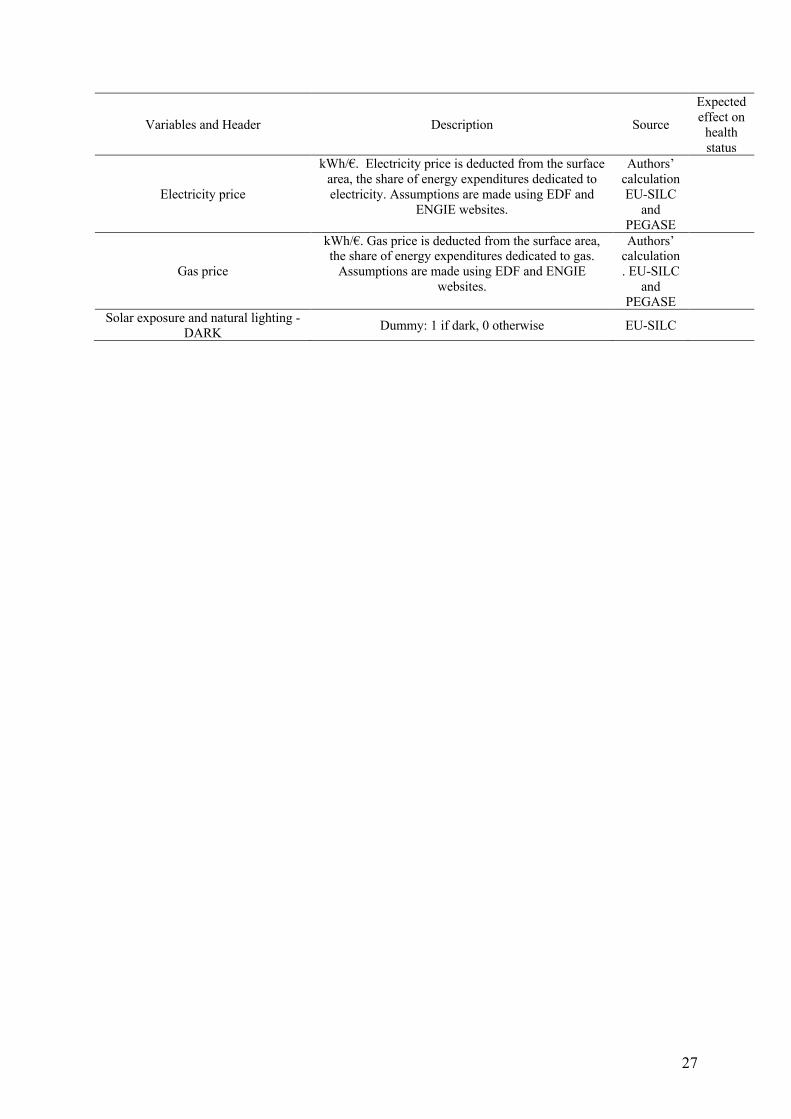
27

Variables and Header Description Source

Expected effect on

health status

Electricity price

kWh/€. Electricity price is deducted from the surface area, the share of energy expenditures dedicated to electricity. Assumptions are made using EDF and

ENGIE websites.

Authors’ calculation EU-SILC

and PEGASE

Gas price

kWh/€. Gas price is deducted from the surface area, the share of energy expenditures dedicated to gas.

Assumptions are made using EDF and ENGIE websites.

Authors’ calculation. EU-SILC

and PEGASE

Solar exposure and natural lighting - DARK Dummy: 1 if dark, 0 otherwise EU-SILC

28

Appendix 2: Theoretical foundations of the empirical strategy

This paper presents an approach based on traditional consumer theory where representation of

individual preferences is based on the bundle of goods they have chosen to maximize their

utility or well-being. So, we characterize individual preferences as 𝑈(𝐺,𝐻).

𝐺 as a whole spectrum of other goods that has nothing to do with medical services and products,

but which definitely contribute to quality of life. Let 𝐻 be the care demand that is directly

derived from a health status h. We assume that a person in good health has a relatively low

health care demand. Then the budget constraint of the individual is simply 𝑚 = 𝑝ℎ𝐻 + 𝑝𝑔𝐺

, where m is just the income of the individual, pg the price of other goods prices and ph the price

of medical care.

The specification of household medical care demand is based on a utility model with R* the

stochastic indirect utility function of the households, which we assume to be unobserved.

Indirect utility V depends on the price of medical care 𝑝ℎ and income m, household

characteristics X, fuel poverty condition FP, climatic and environmental conditions W, and is

defined conditionally on health status j.

Therefore, we have:

𝑅#<∗ = 𝑉#<[𝑝ℎ#,𝑚#, 𝑋#,𝑊#, 𝐹𝑃#] + 𝑣#< (1)

where j=0,1 is health status, i=1, ...., N that of the individual, and vij the error term. The Roy's

identity gives us the household Marshallian demand function for medical care:

𝐻#<(𝑝ℎ#,𝑚, 𝑋#,𝑊#, 𝐹𝑃#) =ijkl(mnk,ok,pk,qk)/imskijkl(mnk,ok,pk,qk)/iok

(2)

𝑝ℎ is the numéraire in the model and equal to 1. In France, the government assumes

responsibility for health expenditures, especially for the poorest households.

On simplification, the medical care demand function conditional on health status j by household

i can be written as follows:

29

𝑞#< = 𝛼#<𝑋#< + 𝛽#<𝑊#< + 𝛾#<𝐹𝑃#< + 𝜂#< (3)

where qij is the quantity of medical care consumed by household i in health status j, Xij is a

vector of household characteristics, Wij is a vector of climatic and environmental conditions,

FPij is the fuel poor variable, 𝛼#<, 𝛽#< and 𝛾#<are vectors of the related parameters, and 𝜂#< the

error term taking into account the influence of unobservable parameters. In our empirical

strategy, we analyzed health status denoted h depending on the same vector variables with a

particular focus on fuel poverty exposure.

Appendix 3: Results

3A – Estimated results for controlling initial conditions To ensure that medical density is a good variable to explain the initial health status, we perform

a Wald test. Based on the p value, we are able to reject the null hypothesis, indicating that the

coefficient for medical density is not equal to zero, meaning that including this variable creates

a statistically significant improvement in the fit of the model at the 1% level.

Table 6 Estimated results for controlling initial conditions

Poor health Chronic disease Coef. St.Err. Sig Coef. St.Err. Sig Fuel poverty 10% 0.246 0.032 *** 0.170 0.027 *** Number of Children 0.039 0.009 *** -0.038 0.006 *** UDD (log) -0.071 0.052 -0.053 0.037 Age 0.027 0.001 *** 0.027 0.000 *** Pollution problem 0.203 0.024 *** 0.174 0.018 *** Undergraduate degree -0.261 0.038 *** -0.079 0.022 *** Homeowner -0.382 0.019 *** -0.176 0.014 *** Medical density -0.001 0.000 *** -0.001 0.000 *** Constant -1.882 0.428 *** -0.752 0.306 ** Observations

45918 45921

Pseudo R-squared

0.117 0.115

Chi-square 3249.936 6953.236 Percent correctly predicted 90.9% 69.5% Wald test chi2( 1) = 7.71 p= 0.0055 chi2( 1) = 62.54 p= 0.0000 LR test chi2( 1) = 7.74 p= 0.0054 chi2( 1) = 62.71 p= 0.0000

*** p<0.01, ** p<0.05, * p<0.1- Bootstrap 5000 replications

3B – Estimated results for binary probit regression on fuel poverty

30

It is quite difficult to test the consistency of instruments. But it is possible to test whether

parameters are significant and significantly improve the fit of the model. In our estimates,

energy prices are significant, especially the price of gas which is significant at 1%. It is also

possible to perform a Wald test, and a likelihood-ratio test. The Wald test performs simple and

composite linear hypotheses about the parameters of the most recently fit model. Based on the

p value, we are able to reject the null hypothesis, indicating that the coefficients for gas price,

electricity price and the interaction parameter for energy prices are not simultaneously equal to

zero, meaning that including these variables creates a statistically significant improvement in

the fit of the model. Finally, the likelihood-ratio test performs a likelihood-ratio test of the null

hypothesis that the parameter vector of a statistical model satisfies some smooth constraint.

Adding the energy price parameters as predictor variables together (not just individually) results

in a statistically significant improvement in the model fit.

Table 7 Estimated results for binary probit regression on fuel poverty

Fuel poverty 10% Fuel poverty LIHC Coef. St.Err. p value Coef. St.Err. p

value

Number of Children -0.156 0.012 *** 0.049 0.010 *** UDD (log) 0.511 0.050 *** 0.183 0.044 *** Age 0.014 0.001 *** 0.005 0.001 *** Pollution problem -0.075 0.028 *** -0.028 0.024 Undergraduate degree

-0.446 0.047 *** -0.498 0.044 ***

Homeowner -0.020 0.026 -0.417 0.022 *** Dark dwelling 0.308 0.030 *** 0.185 0.027 *** Electricity price 1.821 0.328 *** 0.938 0.293 *** Gas price 1.860 1.024 * 5.793 0.906 *** Interaction parameter

0.997 5.949 -19.134 5.285 ***

Constant -7.877 0.388 *** -4.527 0.339 *** Observations 219,404 *** Wald test on electricity price, gas price, darkness and interaction parameter

chi2( 4) = 247.62 p= 0.0000 chi2( 4) = 198.44 p= 0.0000

LR test chi2(3) = 120.62 p= 0.0000 chi2(3) = 143.45 p= 0.0000 Percent correctly predicted 87.2% 86.7%

*** p<0.01, ** p<0.05, * p<0.1 - Bootstrap 5000 replications

3C – Results : probability of being in poor health using the LIHC indicator

31

Table 8 Results - probability of being in poor health using the LIHC indicator

Model 1 Model 2 Model 3 Model 4 Poor health (lag)

1.611*** 1.609***

(0.0328) (0.0328)

Fuel poverty 10% 0.252*** 0.198***

(0.0332) (0.0630)

Number of children 0.0824*** 0.0353*** 0.0188** 0.00461 (0.0127) (0.0118) (0.00857) (0.00607)

Unified Degree Days (log) 0.0527 0.0306 -0.0280 -0.0823*** (0.0466) (0.0361) (0.0371) (0.0252)

Age 0.0529*** 0.0216*** 0.00139 -0.000319 (0.00100) (0.00651) (0.00272) (0.00190)

Pollution problem 0.186*** 0.142*** 0.0202 0.0708*** (0.0247) (0.0515) (0.0273) (0.0179)

Undergraduate degree -0.365*** -0.186*** 0.0287 0.0160 (0.0469) (0.0718) (0.0397) (0.0176)

Homeowner -0.642*** -0.281*** -0.0208 0.00102 (0.0274) (0.0915) (0.0392) (0.0158)

Mills’ ratio

-0.0219 -0.836*** -0.895*** (0.293) (0.119) (0.0994)

Predicted fuel poverty 10%

21.39*** 25.15*** (3.357) (2.964)

Chronic disease (lag)

1.548*** (0.0210)

Constant -5.568*** -3.068*** -0.242 0.526* (0.362) (0.828) (0.431) (0.286)

Observations 173,88 122,362 122,347 122,32 Number of individuals 49,422 37,855 37,855 37,861

*** p<0.01, ** p<0.05, * p<0.1 - Bootstrap 5000 replications

Table 9 Marginal effects of fuel poverty (LIHC) on poor health

Model 1 0.02***

Good health in t-1 Poor health in t-1

Model 2 0.02*** 0.09***

Model 3 2.30*** 8.89***

Model 4 4.38*** 5.62***

*** p<0.01, ** p<0.05, * p<0.1 - Bootstrap 5000 replications

32