analysis of existing bridge for fatigue life · the following classes of live loads as per irc are:...
TRANSCRIPT
http://www.iaeme.com/IJCIET/index.asp 1056 [email protected]
International Journal of Civil Engineering and Technology (IJCIET)
Volume 8, Issue 12, December 2017, pp. 1056–1076, Article ID: IJCIET_08_12_114
Available online at http://http://www.iaeme.com/ijciet/issues.asp?JType=IJCIET&VType=8&IType=12
ISSN Print: 0976-6308 and ISSN Online: 0976-6316
© IAEME Publication Scopus Indexed
ANALYSIS OF EXISTING BRIDGE FOR
FATIGUE LIFE
Vijayashree M
Assistant Professor, Department of Civil Engineering,
Sri Venkateshwara College of Engineering, Bengaluru, India
Shwetha Shetty M R
Assistant Professor, Department of Civil Engineering,
Sri Venkateshwara College of Engineering, Bengaluru, India
Anil Kumar M S
Assistant Professor, Department of Civil Engineering,
Sri Venkateshwara College of Engineering, Bengaluru, India
Santhosh N
Assistant Professor, Department of Civil Engineering,
Sambhram Institute of Technology, Karnataka, India
ABSTRACT
Indian road congress (IRC) recommends a design procedure, prescribed in IRC 21
for design of bridges for flexure. The procedure takes a “Hypothetical vehicles” to be
considered across the bridge for analysis. However in real situation, the vehicles
which move on the bridge are quite different from the hypothetical vehicle considered
in IRC. Hence, this procedure does not reflect the realistic scenario. It is felt that the
effect of movement of real vehicles has to be examined. The bridge when designed
only for flexure may be subjected to premature failure as the concept of fatigue is not
accounted which is an important parameter to be analysed for estimating life of
structure. Considering “Real vehicles” for analysis purpose makes more sense.
“Moving load analysis” conducted to determine the design bending moment will yield
more realistic and reliable data. Hence fatigue analysis is carried out by considering
real vehicles obtained from traffic survey and its implicit factor was found.
Therefore in this work one of the existing bridges have been evaluated for fatigue
life using finite element package as per Indian standard codes.
Key words: cyclic loading, C Program, fatigue, Indian road congress, implicit factor,
load cycles, moving load analysis, rain flow counting, SAP 2000, stress range.
Cite this Article: Vijayashree M, Shwetha Shetty M R, Anil Kumar M S and
Santhosh N, Analysis of Existing Bridge for Fatigue Life. International Journal of
Civil Engineering and Technology, 8(12), 2017, pp. 1056-1076.
http://www.iaeme.com/IJCIET/issues.asp?JType=IJCIET&VType=8&IType=12

Analysis of Existing Bridge for Fatigue Life
http://www.iaeme.com/IJCIET/index.asp 1057 [email protected]
1. INTRODUCTION
Bridge symbolizes the ideas and aspirations of humanity. They are designed differ in the way
they support loads. These loads include the weight of the bridges themselves, the weight of
the material used to build the bridges, and the weight and stresses of the vehicles crossing
them. In flexural analysis for short span bridges or culverts, main loads to be considered are
dead load, live load and impact effect of live loads. For design purpose hypothetical vehicles
as prescribed by IRC is used.
The following classes of live loads as per IRC are:
IRC class AA loading
IRC class A loading
IRC class B loading
1.1. Fatigue
The word „fatigue‟ originated from the Latin expression „fatigue‟ which means „to tire‟. The
phenomenon of fatigue refers to the behaviour of structures under the action of repeated
application of loads. It is a progressive, internal and permanent structural change in the
material. At the beginning of the loading the propagation of the microcracks is rather slow
and as loading continues the micro-cracks will proceed, propagate and lead to macro-cracks,
which may grow further. The macro-cracks determine the remaining fatigue life caused by
stress until failure occurs.
1.2. Different Approaches to Fatigue Analysis
According to the definition of the fatigue life, the approaches for fatigue analysis can be
classified into
The crack propagation method or Fracture Mechanics approach.
The strain-life method and
The stress-life method or S-N curve approach:
The Stress Life, S-N method was the first approach used in attempt to understand and
quantify fatigue. It was the standard fatigue design method for almost 100 years. The S-N
approach is still widely used in design applications.
In order to obtain the curve, each of the tested specimens is exposed to a cyclic loading
with constant amplitude. Then the number of cycles until failure in the specimen is observed.
The logarithm of the number of load cycles to failure, N, at a specific maximum stress level,
σmax is plotted in a diagram. One such curve is valid for a constant ratio between maximum
and minimum stress. To obtain statistically reasonable information for each curve, it is
necessary to test several specimens at each different numbers of cycles to failure.
During the propagation portion of fatigue, damage can be related to crack length. Methods
have been developed which can relate loading sequence to crack extension. The important
point is that during propagation, damage can be related to an observable and measurable
phenomenon. This has been used for a great advantage in the aerospace industry, where
regular inspections are incorporated into the design of damage tolerant structures.
From IRC-58 2011

Vijayashree M, Shwetha Shetty M R, Anil Kumar M S and Santhosh N
http://www.iaeme.com/IJCIET/index.asp 1058 [email protected]
Where SR is stress ratio, N = number of cycles to failure.
1.2.1. Linear damage rule
The linear damage rule was first proposed by Palmgren in 1924 and was further developed by
Miner in 1945.Today,this method is commonly known as Miner‟s Rule. The following
terminology will be used in the discussion
cycle ratio =n/N
Where n is number of cycles at stress level S
N is the fatigue life in cycle at stress level S
The damage fraction D is defined as the fraction of life used up by an event or a series of
events failure in any of the cumulative damage theories is assumed to occur when the
summation of damage fractions equals 1 or ∑Di ≥1
The linear damage rule states that the damage fraction Di, at stress level Si is equal to the
cycle ratio
. For example, the damage fraction D, due to one cycle of loading is
. In
other words, the application of one cycle of loading consumes
of the fatigue life. The
failure criterion for variable amplitude loading can now be stated as ∑
≥ 1
n =
Here Sr-stress level
m – Empirical constant assumed as 3 for concrete.
1.2.2. Load Cycles
A load cycle is a closed loop in “load space”. For harmonic loading, the load cycles starts
from a certain load magnitude, moves through a max-value and a min-value back to the start
magnitude (or the other way around).The load cycle is then completely defined by the
amplitude and mid value.
Figure 1 Harmonic cycle Figure 2 Non harmonic cycle
0
1
2
3
0 20 40 60
stre
ss in
Mp
a
position of load head in meters

Analysis of Existing Bridge for Fatigue Life
http://www.iaeme.com/IJCIET/index.asp 1059 [email protected]
The problem in identifying a load cycle comes when we are not dealing with harmonic
loadpaths. Since the stress variations obtained is of variable amplitudes and the effect of this
is important in fatigue analysis we adopt rainflow counting method.
1.2.3. Cycle Counting
It is necessary to reduce the complex history into a number of events which can be compared
which can be compared to the available constant amplitude test data. This process of reducing
a complex load history into a number of constant amplitude events involves what is termed as
cycle counting.
Counting methods have initially been developed for the study of fatigue damage generated
in aeronautical structures. Since different results have been obtained from different methods,
errors could be taken in the calculations for some of them. Level crossing counting, peak
counting, simple range counting and rain flow counting are the methods which are using
stress or deformation ranges. One of the preferred methods is the rain flow counting method.
The origin of the name of rain flow counting method which is called „Pagoda Roof
Method‟ can be explained as that the time axis is vertical and the random stress S(t) represents
a series of roofs on which waterfalls.
1.2.4. Rain flow Counting
The first step in implementing this procedure is to draw the strain-time history so that the time
is oriented vertically, with increasing time downward. One could now imagine that the strain
history forms a number of “Pogada roofs”. Cycles are then defined by the manner in which
rain is allowed to “drip” or “fall” down the roofs (This is previously mentioned analogy used
by Matsuishi and Endo, from which the rainflow method of cycle counting received its name).
A number of rules are imposed on the dripping rain so as to identify closed hysteresis loops.
The rules specifying the manner in which rain falls are as follows:
To eliminate the counting of half cycles, the strain time history is drawn so as to begin and
end at the strain value of greatest magnitude.
A flow of rain begun at each strain reversal in the history and is allowed to continue to flow
unless:
o The rain began at a local maximum point (peak) and falls opposite a local maximum
point greater than that from which it came.
o The rain began at a local minimum point (valley) and falls opposite to local minimum
point greater (in magnitude) than that from which it came.
o It encounters a previous rainflow.
Figure 3 Example to show rainflow counting

Vijayashree M, Shwetha Shetty M R, Anil Kumar M S and Santhosh N
http://www.iaeme.com/IJCIET/index.asp 1060 [email protected]
As shown in the “Fig 3”, the given strain –time history begins and ends at the strain value
of greatest magnitude (pointA). Rainflow is now initiated at each reversal in the strain history.
A. Rainflow from point A over points B and D and continues to the end of the history since
none of the conditions for stopping rainflow are satisfied.
B. Rainflow from point B over point C and stops opposite point D, since both B and D are
local maximums and the magnitude of D is greater than B(rule 2a)
C. Rainflow from point C and must stop upon meeting the rainflow from point A (rule 2c)
D. Rainflows from point D over points E and G, continues to the end of the history since none
of the conditions for stopping rainflow are satisfied.
E. Rainflows from point E over point F and stops opposite point G, since both E and G are
local minimums and the magnitude of G is greater than E(rule2b)
F. Rainflows from point F and must stops upon meeting the flow from point D(rule2c)
G. Rainflows from point G over point H and stops opposite point A, since both G and A are
local minimums and the magnitude of A is greater than G(rule2b)
H. Rainflows from point H and must stop upon meeting the rainflow from point D(rule2c)
Having completed the above, we are now able to combine events to form completed
cycles. In these example events A-D and D-A are combined to form a full cycle. Event B-C
combines with event C-B (of strain range C-D) to form an additional cycle. Similarly, cycles
are formed at E-F and G-H.
2. CASE STUDY ON A BRIDGE ON NH 169-A ACROSS SWARNA
RIVER IN SHIVAPURA
A Bridge on NH 169-A across Swarna River in Shivapura - Thirthahalli Malpe section and
for the chosen bridge fatigue behavior is studied using S-N approach and life to failure is
determined.
2.1. Objectives
To obtain the maximum bending moment and stresses that bridge would suffer from the
moving load analysis for different composition of traffic using SAP2000.
To find out the fatigue life of the existing reinforced concrete bridge under moving load.
To find out the uncertainty of the bridges by comparing the fatigue life.
To develop C Program to determine the maximum bending moment and stresses that bridge
would suffer from the moving load analysis for different composition of traffic.
To compare variations of the stresses found from C-program and from SAP2000.
To find out the implicit factors by comparing the bending moment at mid span for real
vehicles and hypothetic vehicles as prescribed in IRC for different spans.
Analysis of Existing Bridge for Fatigue Life
http://www.iaeme.com/IJCIET/index.asp 1061 [email protected]
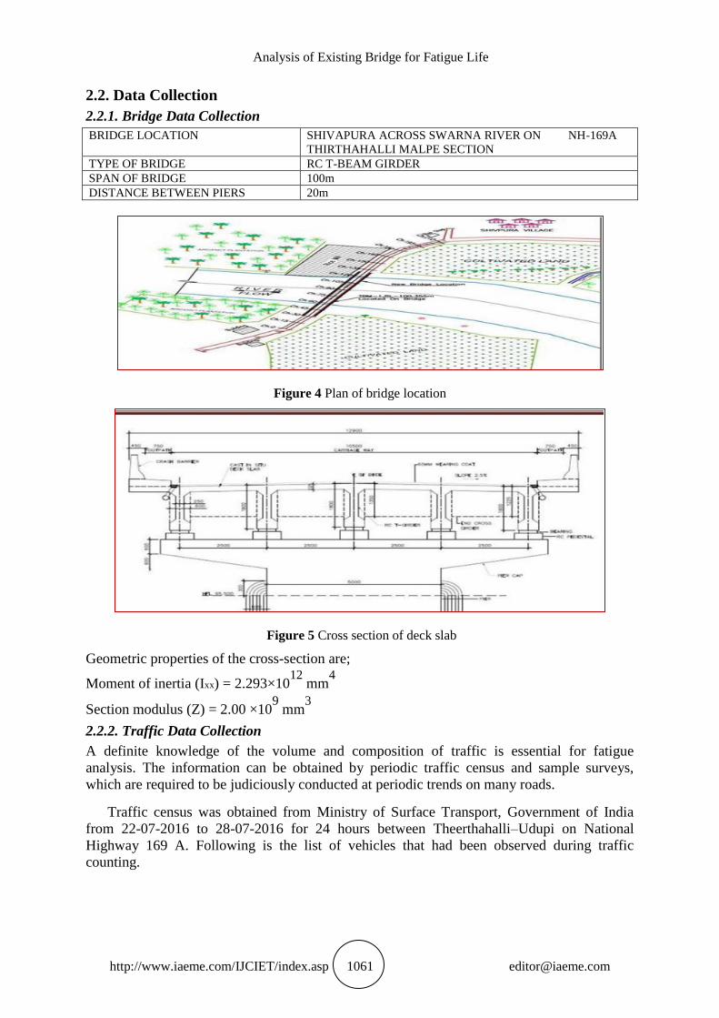
2.2. Data Collection
2.2.1. Bridge Data Collection
BRIDGE LOCATION SHIVAPURA ACROSS SWARNA RIVER ON NH-169A
THIRTHAHALLI MALPE SECTION
TYPE OF BRIDGE RC T-BEAM GIRDER
SPAN OF BRIDGE 100m
DISTANCE BETWEEN PIERS 20m
Figure 4 Plan of bridge location
Figure 5 Cross section of deck slab
Geometric properties of the cross-section are;
Moment of inertia (Ixx) = 2.293×10¹²
mm4
Section modulus (Z) = 2.00 ×109 mm
3
2.2.2. Traffic Data Collection
A definite knowledge of the volume and composition of traffic is essential for fatigue
analysis. The information can be obtained by periodic traffic census and sample surveys,
which are required to be judiciously conducted at periodic trends on many roads.
Traffic census was obtained from Ministry of Surface Transport, Government of India
from 22-07-2016 to 28-07-2016 for 24 hours between Theerthahalli–Udupi on National
Highway 169 A. Following is the list of vehicles that had been observed during traffic
counting.

Vijayashree M, Shwetha Shetty M R, Anil Kumar M S and Santhosh N
http://www.iaeme.com/IJCIET/index.asp 1062 [email protected]
Table 1 List of Vehicles That Had Been Observed During the Traffic Counting
SL NO VEHICLE TYPE NUMBER(PCU)
1 Cars/ Jeeps/ Taxies Van/ Three Wheelers (Auto Rickshaw) 4170
2 Two Wheeler (motor Cycle / Scooter Etc...) 2120
3 LCV (Light Commercial vehicles eg. Mini Truck) 1419
4 Bus 1590
5 Two Axle Trax/Tanker 1197
6 Multi Axle Truck/Truck Trailer/Tanker 652.5
7 Agricultural Tractor / with Trailer 49.5
8 Cycle/Cycle Rickshaw/Other Human Powered 45
9 Bullock Cart / Horse Cart/Other Animal Powered 0
10 Others (Specify) 0
TOTAL 11243
As per IRC: SP: 72 – 2007, The large number of cars, two wheelers and light commercial
vehicles are of little consequence and only the motorized commercial vehicles of gross laden
weight of 3 tones and above (i.e. BS, 2AT and MAT) are to be considered for computation of
design traffic. The details of the vehicles considered along with its specification are tabulated
in “Table 2”.
Table 2 Real Vehicles Considered For the Case Study
Vehicle type BUS (BS) 2AT MAT
vehicle name LPO 1618 LPK 1613 LPK 2518
Wheel base 6.3 m 3.58 m 3.88 m & 4.88 m
Total length of vehicle 12 m 6.365 m 7.08 m
Width of vehicle 2.6 m 2.115 m 2.44 m
Front axle load-FAW (unloaded) 14.4 kN 16 kN 16 kN
Rear axle load-RAW (unloaded) 34 kN 32.1 kN 41.8 kN
Max permissible FAW 54 kN 60 kN 60 kN
Max permissible RAW 108 kN 102 kN 190 kN
Figure 6 LPO 1618 Figure 7 LPK 2518 Figure 8 LPK 1613
2.3. Moving Load Analysis for the Collected Data
In practical situations, live loads such as vehicular loads act on bridges. “The loads whose
position changes with respect to time are called moving load”. By virtue of its motion, such
loads generally induce a dynamic response in the structure. The loads due to the self-weight
of the bridge act at specified points while rolling loads on an account of vehicle passing over
the bridge act at critical points, producing maximum effects.
In the moving loads, when a system of loading crosses a beam, the Shear Force (negative
as well as positive) and Bending Moments at any section of the beam varies as the system of
loads move from one end of the beam to the other end.
Analysis of Existing Bridge for Fatigue Life
http://www.iaeme.com/IJCIET/index.asp 1063 [email protected]
2.3.1. Assumption for Analysis
Critical section is mid span section. The mid span section is assumed to suffer maximum BM
which is usually true.
The slab is simply supported.
Concrete suffers fatigue failure prior to steel.
For the traffic data obtained, following assumptions are made;
The position of the vehicle in lateral direction is not considered.
The load train moving on one lane will exactly occur on the other lane at the same time.
Impact factor = 25 %
The train of loads moves from left to right.
High Speed- 50 Kmph; Low Speed- 25 Kmph
2.3.2. Vehicle Combinations Considered
L - LOADED
UL - UNLOADED
MAT - MULTIAXLED TRUCKS
2AT – TWO AXLED TRUCKS
BS – BUS
Table 3 Vehicles combinations Considered For the Case Study
Vehicle combination high low Vehicle combination high low
LBS+ULBS Case1 Case2 LMAT+ULMAT Case11 Case12
L2AT+UL2AT Case3 Case4 LBS+ULMAT Case13 Case14
LBS+UL2AT Case5 Case6 LMAT+UL2AT Case15 Case16
ULBS+L2AT Case7 Case8 ULBS+LMAT Case17 Case18
L2AT+LBS Case9 Case10 L2AT+ULMAT Case19 Case20
“Table3” shows vehicle combinations and are further considered for two types of
movements:
Scenario 1 high – Fast moving vehicles – 50Kmph vehicle speed (Clear spacing between
vehicles is 2.5 m).
Scenario 2 low– Slow moving vehicles - 25Kmph vehicle speed (Clear spacing between
vehicles is 1.5m)
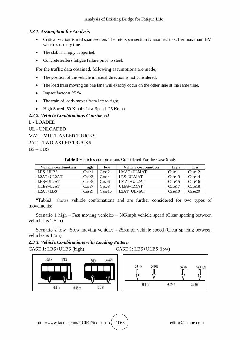
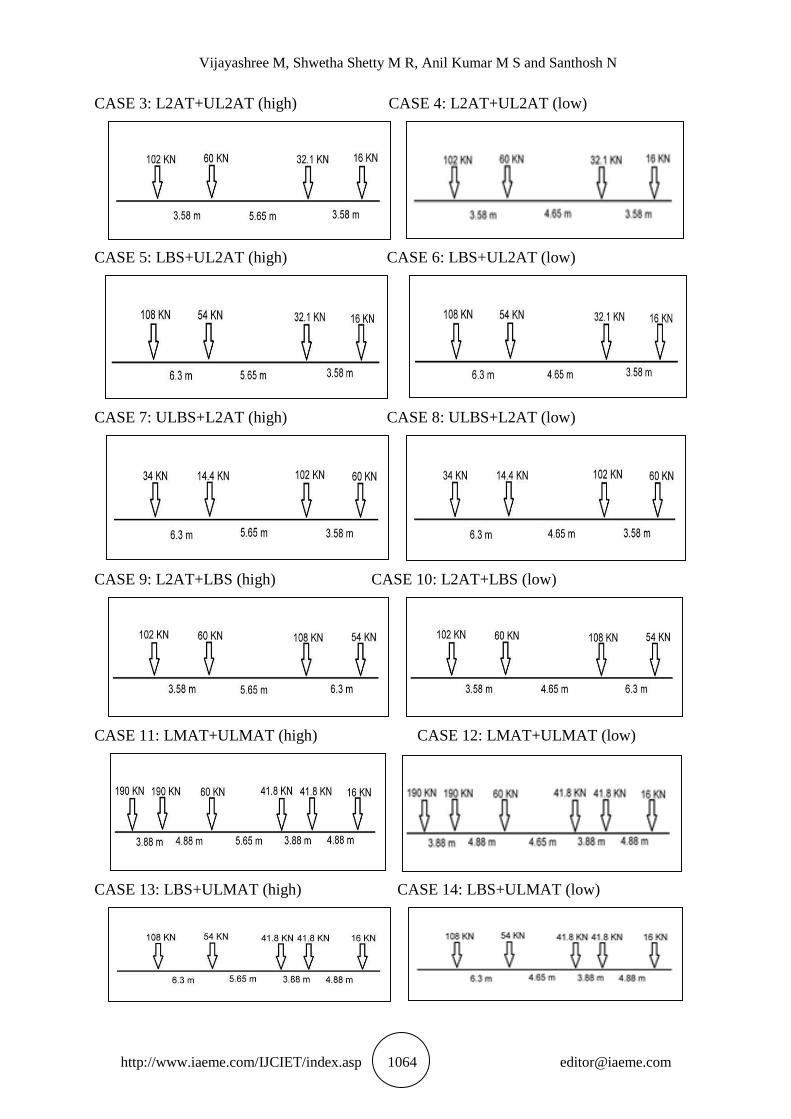
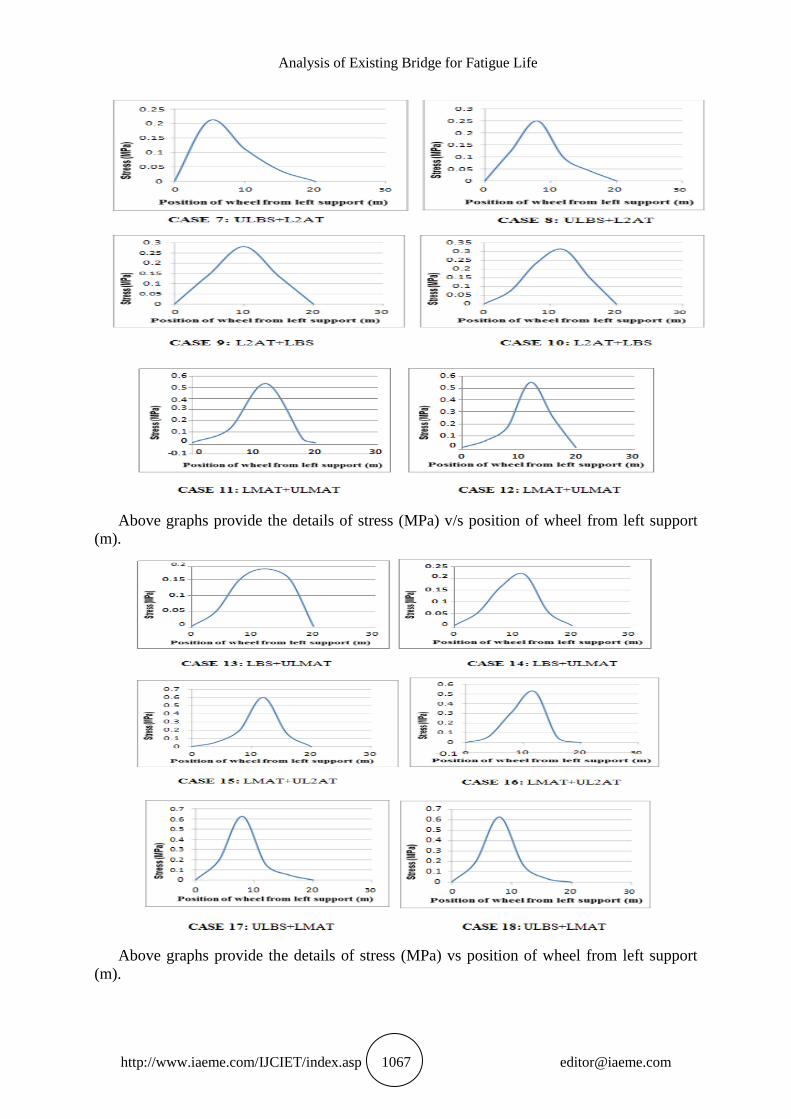
2.3.3. Vehicle Combinations with Loading Pattern
CASE 1: LBS+ULBS (high) CASE 2: LBS+ULBS (low)
Vijayashree M, Shwetha Shetty M R, Anil Kumar M S and Santhosh N
http://www.iaeme.com/IJCIET/index.asp 1064 [email protected]
CASE 3: L2AT+UL2AT (high) CASE 4: L2AT+UL2AT (low)
CASE 5: LBS+UL2AT (high) CASE 6: LBS+UL2AT (low)
CASE 7: ULBS+L2AT (high) CASE 8: ULBS+L2AT (low)
CASE 9: L2AT+LBS (high) CASE 10: L2AT+LBS (low)
CASE 11: LMAT+ULMAT (high) CASE 12: LMAT+ULMAT (low)
CASE 13: LBS+ULMAT (high) CASE 14: LBS+ULMAT (low)

Analysis of Existing Bridge for Fatigue Life
http://www.iaeme.com/IJCIET/index.asp 1065 [email protected]
CASE 15: LMAT+UL2AT (high) CASE 16: LMAT+UL2AT (low)
CASE 17: ULBS+LMAT (high) CASE 18: ULBS+LMAT (low)
CASE 19: L2AT+ULMAT (high) CASE 20: L2AT+ULMAT (low)
2.4. Moving Load Analysis using SAP 2000
Bridge superstructure was modelled in SAP 2000 v-14 which is shown in the “figure 9”. It
consists of three interior girders and two exterior girders. The total width of bridge is 12900
mm which includes crash barrier and foot path. The bridge is provided with two lanes of 3.5
m each.
Figure 9 Bridge Superstructure
2.4.1. Results of Moving Load Analysis
The vehicle combination is defined here on bridge is LBS+ULBS with speed 50 Kmph. This
combination is defined to study Bending Moment and Stress distribution variation on the
entire bridge section. In the moving load analysis, we know that Bending Moment and the
stresses are higher under the load. In the “figure10” the bending moment variation along the

Vijayashree M, Shwetha Shetty M R, Anil Kumar M S and Santhosh N
http://www.iaeme.com/IJCIET/index.asp 1066 [email protected]
bridge section which are obtained from SAP-2000 are shown. From those figures, we can
conclude that SAP-2000 is valid software and can be used for present study.
Moving load analysis is thus done for two types of vehicle movements (fast moving
vehicles and slow moving vehicles). From the obtained bending moment stresses are found
from bending moment equation and are represented graphically in below.
Following are the bending moment diagrams obtained from moving load analysis for the
Case1: LBS+ULBS
Figure 10 Bending moment diagrams obtained from moving load analysis for the Case1: LBS+ULBS
Above graphs provide the details of stress (MPa) vs position of wheel from left support
(m).
Analysis of Existing Bridge for Fatigue Life
http://www.iaeme.com/IJCIET/index.asp 1067 [email protected]
Above graphs provide the details of stress (MPa) v/s position of wheel from left support
(m).
Above graphs provide the details of stress (MPa) vs position of wheel from left support
(m).

Vijayashree M, Shwetha Shetty M R, Anil Kumar M S and Santhosh N
http://www.iaeme.com/IJCIET/index.asp 1068 [email protected]
All the graphs provide the details of stress (MPa) vs position of wheel from left support
(m).Stress values for different vehicle combination which are taken from the graph are shown
in “table 4”.Since the graph follows harmonic loading, cycle is counted as 1.
Table 4 Maximum stress and Cycle obtained for different vehicle combination
Case Vehicle Combinations Speed Cycle Sr Max Mpa
Case 1 LBS+ULBS high 1 0.205
Case 2 LBS+ULBS low 1 0.204
Case 3 L2AT+UL2AT high 1 0.269
Case 4 L2AT+UL2AT low 1 0.266
Case 5 LBS+UL2AT high 1 0.176
Case 6 LBS+UL2AT low 1 0.206
Case 7 ULBS+L2AT high 1 0.21
Case 8 ULBS+L2AT low 1 0.2488
Case 9 L2AT+LBS high 1 0.281
Case 10 L2AT+LBS low 1 0.3125
Case 11 LMAT+ULMAT high 1 0.533
Case 12 LMAT+ULMAT low 1 0.5475
Case 13 LBS+ULMAT high 1 0.186
Case 14 LBS+ULMAT low 1 0.2174
Case 15 LMAT+UL2AT high 1 0.603
Case 16 LMAT+UL2AT low 1 0.524
Case 17 ULBS+LMAT high 1 0.625
Case 18 ULBS+LMAT low 1 0.627
Case19 L2AT+ULMAT high 1 0.2475
Case 20 L2AT+ULMAT low 1 0.2568
2.4.2. Fatigue life calculations (as per the procedure given in the IRC 58)-“equation1”
Considering no growth in traffic:
Let us consider loading case 1: LBS+ULBS
The maximum stress obtained from table; for case 1 is 0.205MPa.
The minimum stress obtained from table; for case 1 is 0 MPa.
= 1 + ∑[SrSr
maxmin
]m
Here, Sr- Stress level; m - Empirical constant assumed as 3 for concrete.
Therefore,
n =1 + [0.2050]3
n= 1.00 cycles
n /year = n*365
= 365 cycles
From IRC: 58 - 2011

Analysis of Existing Bridge for Fatigue Life
http://www.iaeme.com/IJCIET/index.asp 1069 [email protected]
N=unlimited for SR <0.45
N =[
4.4 577
]3.268 When 0.45<=SR<=0.55
SR−0.43
Log10 N =
0.9718−SR
For SR >0.55
0.0828
Where, SR is stress ratio, Nf = Number of cycles to failure.
Here SR =stress caused at maximum load
modulus of rupture of concerte= 0.7*√fck (Assuming fck= 30 MPa) = 3.83 MPa
S R= 0.205/ 3.83= 0.053
Since SR<0.45 therefore assume Nf =2×10⁶
Cumulative damage= ∑ Nfn
Cumulative damage = [20×365
2X10^6] = 0.00365
Life to failure= 273.9726 years.
Similar calculations are carried out for other cases and tabulated as shown in “table5”
Table 5 Two Vehicle Combinations without Traffic Growth
Case Vehicle
Combinations Speed
Cycl
e
Sr
Max
Mpa
n
n/year
(cycles
)
SR
Cum.
Dama
ge
Life
to
failu
re
Case 1 LBS+ULBS high 1 0.205 1 365 0.053
0.0036
5
274
Case 2 LBS+ULBS low 1 0.204 1 365 0.0532
Case 3 L2AT+UL2AT high 1 0.269 1 365 0.07
Case 4 L2AT+UL2AT low 1 0.266 1 365 0.069
Case 5 LBS+UL2AT high 1 0.176 1 365 0.046
Case 6 LBS+UL2AT low 1 0.206 1 365 0.054
Case 7 ULBS+L2AT high 1 0.21 1 365 0.055
Case 8 ULBS+L2AT low 1 0.2488 1 365 0.065
Case 9 L2AT+LBS high 1 0.281 1 365 0.073
Case 10 L2AT+LBS low 1 0.3125 1 365 0.082
Case 11 LMAT+ULMAT high 1 0.533 1 365 0.139
Case 12 LMAT+ULMAT low 1 0.5475 1 365 0.143
Case 13 LBS+ULMAT high 1 0.186 1 365 0.049
Case 14 LBS+ULMAT low 1 0.2174 1 365 0.057
Case 15 LMAT+UL2AT high 1 0.603 1 365 0.157
Case 16 LMAT+UL2AT low 1 0.524 1 365 0.137
Case 17 ULBS+LMAT high 1 0.625 1 365 0.163
Case 18 ULBS+LMAT low 1 0.627 1 365 0.164
Case19 L2AT+ULMAT high 1 0.2475 1 365 0.065
Case 20 L2AT+ULMAT low 1 0.2568 1 365 0.067

Vijayashree M, Shwetha Shetty M R, Anil Kumar M S and Santhosh N
http://www.iaeme.com/IJCIET/index.asp 1070 [email protected]
Table 6 Two Vehicle Combinations with 25 years of traffic Growth
Case Vehicle Combinations Speed Cycle Sr Max
Mpa n
n/year
(cycles) SR
Cum.
Damage
Life
to
failur
e
Case 1 LBS+ULBS high 13.5 0.205 1 4927.5 0.053
0.0092 109
Case 2 LBS+ULBS low 32.2 0.204 1 11763.9 0.053
Case 3 L2AT+UL2AT high 8.55 0.269 1 3122.5 0.07
Case 4 L2AT+UL2AT low 20.4 0.266 1 7456.03 0.069
Case 5 LBS+UL2AT high 22 0.176 1 8048.3 0.046
Case 6 LBS+UL2AT low 52.6 0.206 1 19216.3 0.054
Case 7 ULBS+L2AT high 22 0.21 1 8048.25 0.055
Case 8 ULBS+L2AT low 52.6 0.2488 1 19216.3 0.065
Case 9 L2AT+LBS high 22 0.281 1 8048.3 0.073
Case 10 L2AT+LBS low 52.3 0.3125 1 19246.3 0.082
Case 11 LMAT+ULMAT high 3.37 0.533 1 1230.96 0.139
Case 12 LMAT+ULMAT low 8.05 0.5475 1 2940.9 0.143
Case 13 LBS+ULMAT high 6.8 0.186 1 6157.3 0.049
Case 14 LBS+ULMAT low 40.2 0.2174 1 14702.2 0.057
Case 15 LMAT+UL2AT high 11.9 0.603 1 4354.5 0.157
Case 16 LMAT+UL2AT low 28.4 0.524 1 10397 0.137
Case 17 ULBS+LMAT high 16.8 0.625 1 6157.6 0.163
Case 18 ULBS+LMAT low 40.28 0.627 1 14702.2 0.164
Case19 L2AT+ULMAT high 11.93 0.2475 1 4354.5 0.065
Case 20 L2AT+ULMAT low 28 0.2568 1 10397 0.037
Table 7 Two Vehicle Combinations with 50 years of traffic Growth
Case Vehicle
Combinations Speed Cycle
Sr
Max
Mpa
n n/year
(cycles) SR
Cum.
Damage
Life
to
failur
e
Case 1 LBS+ULBS high 82.3 0.205 1 30039.5 0.053
0.03883
26
Case 2 LBS+ULBS low 196.5 0.204 1 71722.5 0.0532
Case 3 L2AT+UL2AT high 52.2 0.269 1 19042.96 0.07
Case 4 L2AT+UL2AT low 124.6 0.266 1 45468.96 0.069
Case 5 LBS+UL2AT high 134.5 0.176 1 49080.64 0.046
Case 6 LBS+UL2AT low 3.21 0.206 1 1171.65 0.054
Case 7 ULBS+L2AT high 134.46 0.21 1 49080.64 0.055
Case 8 ULBS+L2AT low 3.21 0.2488 1 1171.65 0.065
Case 9 L2AT+LBS high 134.46 0.281 1 49080.64 0.073
Case 10 L2AT+LBS low 3.21 0.3125 1 1171.65 0.082
Case 11 LMAT+ULMAT high 20.56 0.533 1 7509.875 0.139
Case 12 LMAT+ULMAT low 49.13 0.5475 1 17932.45 0.143
Case 13 LBS+ULMAT high 102.87 0.186 1 37547.55 0.049
Case 14 LBS+ULMAT low 245.63 0.2174 1 89654.04 0.057
Case 15 LMAT+UL2AT high 72.745 0.603 1 26551.93 0.157
Case 16 LMAT+UL2AT low 173.7 0.524 1 63397.76 0.137
Case 17 ULBS+LMAT high 102.87 0.625 1 37547.55 0.163
Case 18 ULBS+LMAT low 245.63 0.627 1 89654.04 0.164
Case19 L2AT+ULMAT high 72.745 0.2475 1 26551.93 0.065
Case 20 L2AT+ULMAT low 173.7 0.2568 1 63397.76 0.067
2.5. Moving load analysis using C Program
Program to carryout moving load analysis is shown below:
#include<stdio.h>
#include<conio.h>
Void main ()
{
int n,i;

Analysis of Existing Bridge for Fatigue Life
http://www.iaeme.com/IJCIET/index.asp 1071 [email protected]
float p[10],l,c,a,x[10],m[10],t=0,y;
printf("enter the span\n");
scanf("%f",&l);
printf("enter number of loads\n");
scanf("%d",&n);
for(i=0;i<n;i++)
{
printf("enter the weights of the loads %d \n",i+1); scanf("%f",&p[i]);
printf("enter the distance of load %d \n",i+1);
scanf("%f",&x[i]);
}
c=l/2;
printf("enter the increment length \n");
scanf("%f",&a);
x[0]=x[0]-a;
for(i=0;i<n;i++)
{
x[i]=x[0]-x[i];
}
y=x[n-1];
while(y<=l)
{
for(i=0;i<n;i++)
{
if(x[i]>=0 && x[i]<=c)
{
m[i]=t+((p[i]*x[i]*(l-c))/l);
t=m[i];
//printf("t 1st condition is %f\n",t);
}
else if(x[i]>c && x[i]<=l)
{
m[i]=t+((p[i]*(l-x[i])*c)/l);
t=m[i];
//printf("t 2nd condition is %f\n",t);
}
else
{
m[i]=0;
//printf("t 3rd condition is %f\n",t);
}
Vijayashree M, Shwetha Shetty M R, Anil Kumar M S and Santhosh N
http://www.iaeme.com/IJCIET/index.asp 1072 [email protected]
}
printf("bending moment at this iteration is %f\n",t);
t=0;
y=y+a;
for(i=0;i<n;i++)
{
x[i]=x[i]+a;
}
}
getch();
}
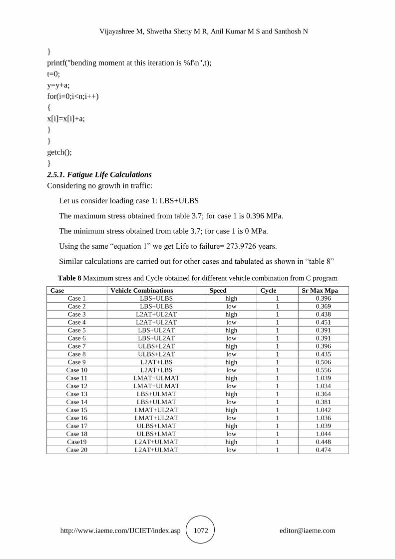
2.5.1. Fatigue Life Calculations
Considering no growth in traffic:
Let us consider loading case 1: LBS+ULBS
The maximum stress obtained from table 3.7; for case 1 is 0.396 MPa.
The minimum stress obtained from table 3.7; for case 1 is 0 MPa.
Using the same “equation 1” we get Life to failure= 273.9726 years.
Similar calculations are carried out for other cases and tabulated as shown in “table 8”
Table 8 Maximum stress and Cycle obtained for different vehicle combination from C program
Case Vehicle Combinations Speed Cycle Sr Max Mpa
Case 1 LBS+ULBS high 1 0.396
Case 2 LBS+ULBS low 1 0.369
Case 3 L2AT+UL2AT high 1 0.438
Case 4 L2AT+UL2AT low 1 0.451
Case 5 LBS+UL2AT high 1 0.391
Case 6 LBS+UL2AT low 1 0.391
Case 7 ULBS+L2AT high 1 0.396
Case 8 ULBS+L2AT low 1 0.435
Case 9 L2AT+LBS high 1 0.506
Case 10 L2AT+LBS low 1 0.556
Case 11 LMAT+ULMAT high 1 1.039
Case 12 LMAT+ULMAT low 1 1.034
Case 13 LBS+ULMAT high 1 0.364
Case 14 LBS+ULMAT low 1 0.381
Case 15 LMAT+UL2AT high 1 1.042
Case 16 LMAT+UL2AT low 1 1.036
Case 17 ULBS+LMAT high 1 1.039
Case 18 ULBS+LMAT low 1 1.044
Case19 L2AT+ULMAT high 1 0.448
Case 20 L2AT+ULMAT low 1 0.474
Analysis of Existing Bridge for Fatigue Life
http://www.iaeme.com/IJCIET/index.asp 1073 [email protected]
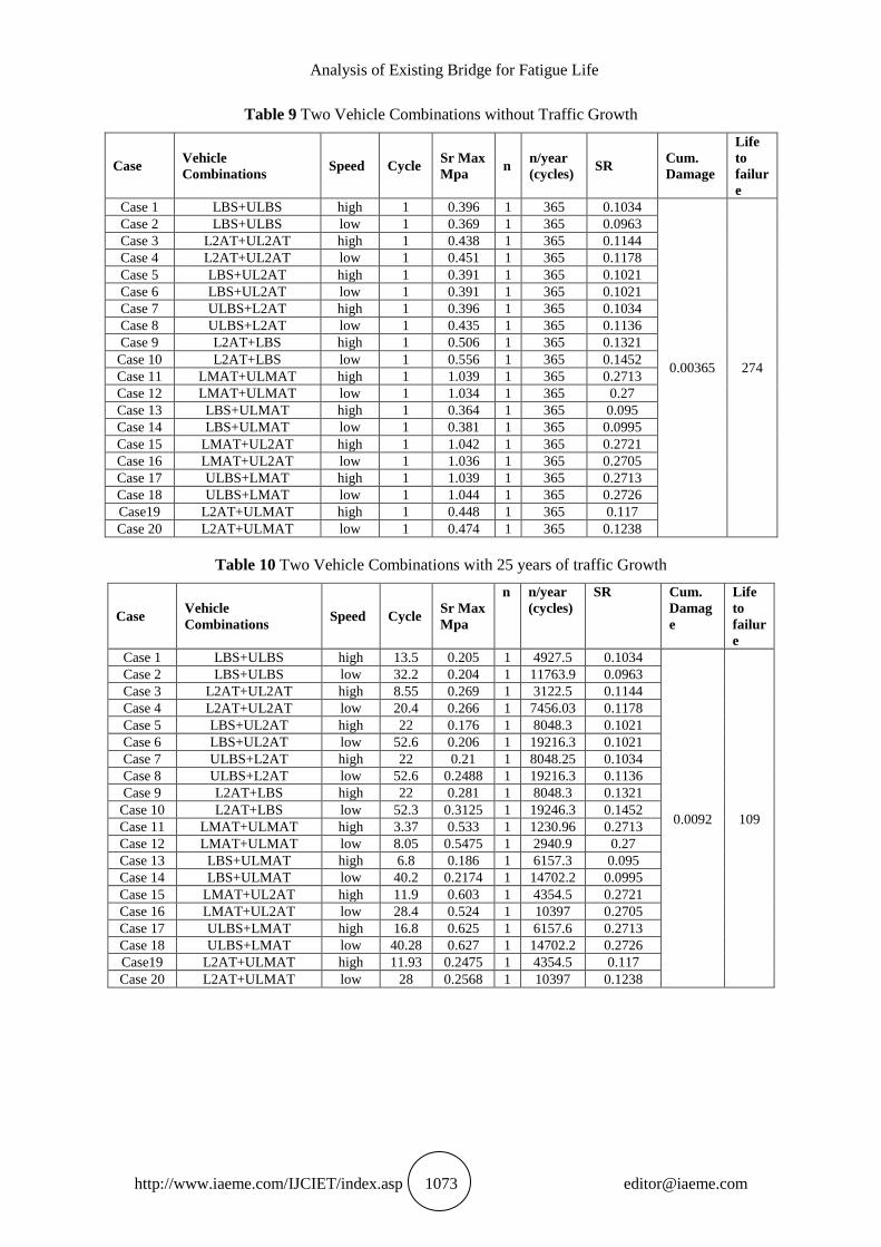
Table 9 Two Vehicle Combinations without Traffic Growth
Case Vehicle
Combinations Speed Cycle
Sr Max
Mpa n
n/year
(cycles) SR
Cum.
Damage
Life
to
failur
e
Case 1 LBS+ULBS high 1 0.396 1 365 0.1034
0.00365 274
Case 2 LBS+ULBS low 1 0.369 1 365 0.0963
Case 3 L2AT+UL2AT high 1 0.438 1 365 0.1144
Case 4 L2AT+UL2AT low 1 0.451 1 365 0.1178
Case 5 LBS+UL2AT high 1 0.391 1 365 0.1021
Case 6 LBS+UL2AT low 1 0.391 1 365 0.1021
Case 7 ULBS+L2AT high 1 0.396 1 365 0.1034
Case 8 ULBS+L2AT low 1 0.435 1 365 0.1136
Case 9 L2AT+LBS high 1 0.506 1 365 0.1321
Case 10 L2AT+LBS low 1 0.556 1 365 0.1452
Case 11 LMAT+ULMAT high 1 1.039 1 365 0.2713
Case 12 LMAT+ULMAT low 1 1.034 1 365 0.27
Case 13 LBS+ULMAT high 1 0.364 1 365 0.095
Case 14 LBS+ULMAT low 1 0.381 1 365 0.0995
Case 15 LMAT+UL2AT high 1 1.042 1 365 0.2721
Case 16 LMAT+UL2AT low 1 1.036 1 365 0.2705
Case 17 ULBS+LMAT high 1 1.039 1 365 0.2713
Case 18 ULBS+LMAT low 1 1.044 1 365 0.2726
Case19 L2AT+ULMAT high 1 0.448 1 365 0.117
Case 20 L2AT+ULMAT low 1 0.474 1 365 0.1238
Table 10 Two Vehicle Combinations with 25 years of traffic Growth
Case Vehicle
Combinations Speed Cycle
Sr Max
Mpa
n n/year
(cycles)
SR Cum.
Damag
e
Life
to
failur
e
Case 1 LBS+ULBS high 13.5 0.205 1 4927.5 0.1034
0.0092
109
Case 2 LBS+ULBS low 32.2 0.204 1 11763.9 0.0963
Case 3 L2AT+UL2AT high 8.55 0.269 1 3122.5 0.1144
Case 4 L2AT+UL2AT low 20.4 0.266 1 7456.03 0.1178
Case 5 LBS+UL2AT high 22 0.176 1 8048.3 0.1021
Case 6 LBS+UL2AT low 52.6 0.206 1 19216.3 0.1021
Case 7 ULBS+L2AT high 22 0.21 1 8048.25 0.1034
Case 8 ULBS+L2AT low 52.6 0.2488 1 19216.3 0.1136
Case 9 L2AT+LBS high 22 0.281 1 8048.3 0.1321
Case 10 L2AT+LBS low 52.3 0.3125 1 19246.3 0.1452
Case 11 LMAT+ULMAT high 3.37 0.533 1 1230.96 0.2713
Case 12 LMAT+ULMAT low 8.05 0.5475 1 2940.9 0.27
Case 13 LBS+ULMAT high 6.8 0.186 1 6157.3 0.095
Case 14 LBS+ULMAT low 40.2 0.2174 1 14702.2 0.0995
Case 15 LMAT+UL2AT high 11.9 0.603 1 4354.5 0.2721
Case 16 LMAT+UL2AT low 28.4 0.524 1 10397 0.2705
Case 17 ULBS+LMAT high 16.8 0.625 1 6157.6 0.2713
Case 18 ULBS+LMAT low 40.28 0.627 1 14702.2 0.2726
Case19 L2AT+ULMAT high 11.93 0.2475 1 4354.5 0.117
Case 20 L2AT+ULMAT low 28 0.2568 1 10397 0.1238
Vijayashree M, Shwetha Shetty M R, Anil Kumar M S and Santhosh N
http://www.iaeme.com/IJCIET/index.asp 1074 [email protected]
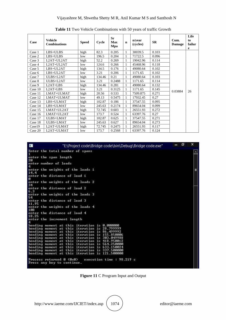
Table 11 Two Vehicle Combinations with 50 years of traffic Growth
Case Vehicle
Combinations Speed Cycle
Sr
Max
Mpa
n n/year
(cycles) SR
Cum.
Damage
Life
to
failur
e
Case 1 LBS+ULBS high 82.3 0.205 1 30039.5 0.103
0.03884
26
Case 2 LBS+ULBS low 196.5 0.204 1 71722.5 0.096
Case 3 L2AT+UL2AT high 52.2 0.269 1 19042.96 0.114
Case 4 L2AT+UL2AT low 124.6 0.266 1 45468.96 0.118
Case 5 LBS+UL2AT high 134.5 0.176 1 49080.64 0.102
Case 6 LBS+UL2AT low 3.21 0.206 1 1171.65 0.102
Case 7 ULBS+L2AT high 134.46 0.21 1 49080.64 0.103
Case 8 ULBS+L2AT low 3.21 0.2488 1 1171.65 0.114
Case 9 L2AT+LBS high 134.46 0.281 1 49080.64 0.132
Case 10 L2AT+LBS low 3.21 0.3125 1 1171.65 0.145
Case 11 LMAT+ULMAT high 20.56 0.533 1 7509.875 0.271
Case 12 LMAT+ULMAT low 49.13 0.5475 1 17932.45 0.27
Case 13 LBS+ULMAT high 102.87 0.186 1 37547.55 0.095
Case 14 LBS+ULMAT low 245.63 0.2174 1 89654.04 0.099
Case 15 LMAT+UL2AT high 72.745 0.603 1 26551.93 0.272
Case 16 LMAT+UL2AT low 173.7 0.524 1 63397.76 0.27
Case 17 ULBS+LMAT high 102.87 0.625 1 37547.55 0.271
Case 18 ULBS+LMAT low 245.63 0.627 1 89654.04 0.273
Case19 L2AT+ULMAT high 72.745 0.2475 1 26551.93 0.117
Case 20 L2AT+ULMAT low 173.7 0.2568 1 63397.76 0.124
Figure 11 C Program Input and Output
Analysis of Existing Bridge for Fatigue Life
http://www.iaeme.com/IJCIET/index.asp 1075 [email protected]
3. RESULTS AND DISCUSSIONS
The results for the case study on the Bridge on NH 169-A across Swarna River in Shivapura -
Thirthahalli Malpe section and for the chosen bridge fatigue behavior is studied using S-N
approach and life to failure is determined and also the results are compared and validated by
using SAP 2000 Software and C –program.
3.1. Fatigue Life Comparison
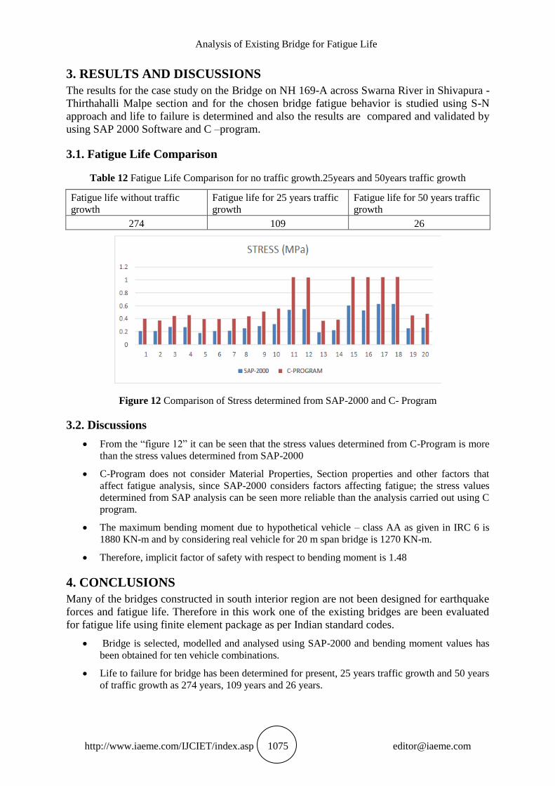
Table 12 Fatigue Life Comparison for no traffic growth.25years and 50years traffic growth
Fatigue life without traffic
growth
Fatigue life for 25 years traffic
growth
Fatigue life for 50 years traffic
growth
274 109 26
Figure 12 Comparison of Stress determined from SAP-2000 and C- Program
3.2. Discussions
From the “figure 12” it can be seen that the stress values determined from C-Program is more
than the stress values determined from SAP-2000
C-Program does not consider Material Properties, Section properties and other factors that
affect fatigue analysis, since SAP-2000 considers factors affecting fatigue; the stress values
determined from SAP analysis can be seen more reliable than the analysis carried out using C
program.
The maximum bending moment due to hypothetical vehicle – class AA as given in IRC 6 is
1880 KN-m and by considering real vehicle for 20 m span bridge is 1270 KN-m.
Therefore, implicit factor of safety with respect to bending moment is 1.48
4. CONCLUSIONS
Many of the bridges constructed in south interior region are not been designed for earthquake
forces and fatigue life. Therefore in this work one of the existing bridges are been evaluated
for fatigue life using finite element package as per Indian standard codes.
Bridge is selected, modelled and analysed using SAP-2000 and bending moment values has
been obtained for ten vehicle combinations.
Life to failure for bridge has been determined for present, 25 years traffic growth and 50 years
of traffic growth as 274 years, 109 years and 26 years.

Vijayashree M, Shwetha Shetty M R, Anil Kumar M S and Santhosh N
http://www.iaeme.com/IJCIET/index.asp 1076 [email protected]
The reasons for reduction in life to failure towards increase in traffic growth are mainly due to
increase in cyclic loading.
C program has been developed to carryout moving load analysis for case study and respective
stress values are determined for different vehicular combinations and obtained results is found
almost twice that of stress values determined from SAP.
The reason for variation in stress in two methods of analysis is mainly due to factors that
affect fatigue life such as material property, stress ratio, cycle to failure, section property etc.
Implicit factor of safety for case study with respect to bending moment is 1.48
REFERENCES
[1] Mohammad Reza Saberi, Bridge Fatigue Service-Life Estimation Using Operational
Strain Measurement, 10.1061/(ASCE)BE.1943-5592.0000860-2016
[2] HabeebaA, Sabeena M.V, Anjusha R, Fatigue Evaluation of Reinforced Concrete
Highway Bridge, Vol. 4, Issue 4- April 2015
[3] Dr. Raquib Ahsan ,Fatigue in Concrete Structures (2013)
[4] Patrick Fehlmannand Thomas, Experimental Investigations on the Fatigue
[5] Behavior of Concrete Bridges, IABSE Reports, Vol. 96- 2009
[6] W. Derkowski, Fatigue life of reinforced concrete beams under bending strengthened with
composite materials, Vol. 6-2006
[7] R Ranganathan, Reliability analysis and design of structures
[8] Indian Road Congress (IRC) 6:2010, Standard Specifications and Code of Practice for
Road Bridges
[9] Indian Road Congress (IRC) (2002) IRC 58, Guidelines for design of rigid pavements,
Indian Road Congress, New Delhi, India
[10] Indian Road Congress (IRC) 21-2000, Standard Specifications and Code of Practice for
Road Bridges
[11] Indian Road Congress (IRC) 9-1972 Traffic census on non-urban roads, Indian Road
Congress, New Delhi, India
[12] Satyam Kumar, Dr. Uday Krishna Ravella , Atul Kuma r Shrivastava, Dr.Midathoda Anil
and Dr. S. K. Kumar Swamy A Review on Human Cervical Fatigue Measurement
Technologies and Data Analysis Methods. International Journal of Mechanical
Engineering and Technology, 8(7), 2017, pp. 1474–1484.
[13] D. Rajesh, V. Balaji, A. Devaraj and D. Yogaraj. An Investigation on Effects of Fatigue
Load on Vibration Characteristics of Woven Fabric Glass/Carbon Hybrid Composite
Beam under Fixed-Free End Condition using Finite Element Method. International
Journal of Mechanical Engineering and Technology, 8(7), 2017, pp. 85–91