analysis of kinect for mobile robots (unofficial kinect data sheet on page 27)
DESCRIPTION
Contains an unofficial Kinect-datasheet which has proven to be useful for others working with this sensor (p27).TRANSCRIPT

Mikkel Viager
Analysis of Kinect for mobile robots Individual course report, March 2011


Mikkel Viager
Analysis of Kinect for mobile robots Individual course report, March 2011

Analysis of Kinect for mobile robots Report written by: Mikkel Viager Advisor: Jens Christian Andersen
DTU Electrical Engineering Technical University of Denmark 2800 Kgs. Lyngby Denmark [email protected]
Project period:
10/02/2011 - 14/03/ 2011
ECTS:
5 Points
Education:
M. Science
Field:
Electrical Engineering
Class:
Public
Remarks:
This report is submitted as partial fulfillment of the requirements for graduation in the above education at the Technical University of Denmark.
Copyrights: © Mikkel Viager, 2011

Analysis of kinect for mobile robots Mi 5
Mikkel Viager, March 2011
Abstract
Through this project, a data sheet containing more detailed specifications on the pre-
cision of the Kinect, than are available from official sources, has been created. Fur-
thermore, an evaluation of several important aspects when considering the use of
Kinect for mobile robots has been conducted, making it possible to conclude that the
Kinect is to be considered as a very viable choice for use with mobile robots.

6 Analysis of kinect for mobile robots .
Mikkel Viager, March 2011
Resumé Ved udførelsen af dette projekt er sammensat et datablad indeholdende detaljerede
informationer om Kinect-sensorens specifikationer, som ikke er tilgængelige fra offi-
cielle kilder. Yderligere er vigtige aspekter, i forbindelse med brug af Kinect for mobile
robotter, blevet gennemgået. Dette har ført til konklusionen at Kinect er en særdeles
brugbar sensor-løsning til anvendelse i forbindelse med mobile robotter.

Analysis of kinect for mobile robots Mi 7
Mikkel Viager, March 2011
Table of Contents 1. Introduction .............................................................................................................. 9
1.1 Documentation overview .................................................................................... 9
2. Light Coding with the Kinect .................................................................................. 11
3. Spatial and depth resolution ................................................................................... 13
3.1 Spatial X and Y resolution .................................................................................. 15
3.2 Depth resolution................................................................................................ 16
4. Actual distance from sensor value ...........................................................................17
5. Interference caused by multiple Kinects ................................................................. 19
5.1 Overlapping of projected IR-patterns ................................................................ 19
5.2 Further work ...................................................................................................... 20
6. General considerations ........................................................................................... 21
6.1 Field of View ...................................................................................................... 21
6.2 Hardware .......................................................................................................... 22
6.3 Power consumption .......................................................................................... 23
6.4 Robustness ........................................................................................................ 23
6.5 Outdoor use ...................................................................................................... 23
7. Conclusion .............................................................................................................. 25
Appendix A ................................................................................................................. 27
Appendix B ................................................................................................................. 29
Appendix C ................................................................................................................. 31
Appendix D ................................................................................................................. 33
Appendix E ................................................................................................................. 35
References...................................................................................................................37
CD Contents ............................................................................................................... 39
Treat_data.m – MATLAB code ................................................................................... 40


Analysis of kinect for mobile robots Mi 9
Mikkel Viager, March 2011
1. Introduction
In order to successfully navigate a mobile robot, obtaining detailed information on the
robots’ immediate environment is a main concern. If the collected data is correct and
sufficiently detailed, developers are given the opportunity to create accordingly so-
phisticated navigation software.
Numerous sensor technologies are available, and they each provide unique advantag-
es for use in specific environments or situations. In addition to sensor types, the de-
sired number of dimensions to track can vary. A simple range finder can detect a dis-
tance in 1 dimension, and more complex scanners can do 2D or 3D scan sweeps. Whe-
reas an additional dimension greatly increases the detail and overall usability of the
collected data, it also causes a major leap in the purchasing price of the sensor.
Recently a whole new type of sensor technology called Light Coding has become
available for purchase at only a small fraction of the price of other 3D range finders.
The technology has been developed by the company PrimeSense [1], and is currently
implemented and sold by Microsoft in the “Kinect” for the game console Xbox 360.
The goal of this project is to analyse the usability of the Kinect for mobile robots, by
evaluating the ability of robust data collection and general applicability to this field.
All test and measurements have been carried out in Linux on the Mobotware[2] plat-
form, with a plugin based on open source Kinect drivers [3].
1.1 Documentation overview
This report is mainly focused on the produced data sheet in Appendix A. Thus, all main
results can be derived from plots and values presented there.
For details on how the measurements were made, as well as evaluation of the results
obtained, the following chapters will provide an overview.
Chapter 2: A brief explanation on how Light Coding works.
Chapter 3: Determining the resolution accuracy for spatial X/Y and depth Z coord.
Chapter 4: Finding the relation between sensor value and actual distance.
Chapter 5: Interference from use of multiple Kinects in the same environment.
Chapter 6: Other considerations of relevance when using Kinect for mobile robots.
Chapter 7: Conclusion
Appendix A: Data sheet


Analysis of kinect for mobile robots Mi 11
Mikkel Viager, March 2011
2. Light Coding with the Kinect Many current range-finding technologies uses time-of-flight to determine the dis-
tance to an object by measuring the time it takes for a flash of light to travel to and
reflect back from its surface. Light Coding uses an entirely different approach where
the light source is constantly turned on, greatly reducing the need for precision timing
of the measurements.
A laser source emits invisible light (approximately at the infrared wavelength) which
passes through a filter and is scattered into a semi-random but constant pattern of
small dots which is projected onto the environment in front of the sensor. The reflect-
ed pattern is then detected by an infrared (IR) camera and analyzed. In Figure 1 the
sensor and the projected light pattern is shown on an image taken with an IR camera.
Figure 1: The projected infrared pattern [5].
Supported by the nine brighter dots in the centers of the slightly noticeable checker-
pattern, the reflection of each dot is evaluated on its position. From knowledge on the
emitted light pattern, lens distortion, and distance between emitter and receiver, the
distance to each dot can be estimated by calculation. To achieve a rate of 30 com-
pleted scans per second, the process makes use of values from neighboring points.
This is done internally in the Kinect, and the final depth image is directly available.


Analysis of kinect for mobile robots Mi 13
Mikkel Viager, March 2011
3. Spatial and depth resolution
The specifications given with the reference model from PrimeSense on the depth im-
age resolution is only for 2m distance measurements. At this range is given both spa-
tial x/y resolution, as well as depth (z) resolution. The provided values at 2m are shown
below in Table 1.
Spatial x/y resolution (@ 2m distance) 3mm
Depth z resolution (@ 2m distance) 1cm
Table 1: Provided resolution values for PrimeSense reference model
This very limited information is insufficient for evaluation in this case, as the resolu-
tion can be expected to vary with distance.
By collecting measurement data for various distances, a better insight in the resolu-
tion properties has been uncovered. The setup for the experiments is shown in Figure
2 (the corresponding depth scan can be found in Appendix B)
Figure 2: Experiment setup
The Kinect sensor is kept at a stationary point, and a flat plate colored semi-matte
white of size 378 x 392mm (h x w) is placed (and vertically leveled) at measured dis-
tances. Because of the floor surface being a white carpet, the sensor is not able to get
any usable reflections from it, making extraction of data for only the plate relatively

14 Analysis of kinect for mobile robots .
Mikkel Viager, March 2011
easy. Once extracted, the data is ported to MATLAB for further analysis. An example
of depth data for the plate is shown in Figure 3, where a color gradient is used to vi-
sualize the depth values.
Figure 3: Depth data for the plate at a distance of 1.2m
At distances of below 1m, the reflection in the center of the plate was too bright to be
properly detected. This is due to reflective properties of the white surface, and is es-
timated to have only a minor impact on the results. An example of this can be seen on
the picture in Appendix B, or by plotting the measurement data using the MATLAB
file on the CD.
A total of 40 such measurements were taken, in 0.1m interval from 0.6m to 4.6m. The
overall interval is chosen to be greater than the 0.8-3.5m operation interval suggested
by PrimeSense, in order to also see if these boundaries are reasonable.
Analysis of kinect for mobile robots Mi 15
Mikkel Viager, March 2011
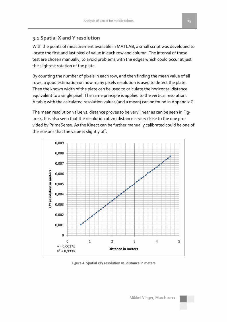
3.1 Spatial X and Y resolution
With the points of measurement available in MATLAB, a small script was developed to
locate the first and last pixel of value in each row and column. The interval of these
test are chosen manually, to avoid problems with the edges which could occur at just
the slightest rotation of the plate.
By counting the number of pixels in each row, and then finding the mean value of all
rows, a good estimation on how many pixels resolution is used to detect the plate.
Then the known width of the plate can be used to calculate the horizontal distance
equivalent to a single pixel. The same principle is applied to the vertical resolution.
A table with the calculated resolution values (and a mean) can be found in Appendix C.
The mean resolution value vs. distance proves to be very linear as can be seen in Fig-
ure 4. It is also seen that the resolution at 2m distance is very close to the one pro-
vided by PrimeSense. As the Kinect can be further manually calibrated could be one of
the reasons that the value is slightly off.
Figure 4: Spatial x/y resolution vs. distance in meters
y = 0,0017x
R² = 0,9998
0
0,001
0,002
0,003
0,004
0,005
0,006
0,007
0,008
0,009
0 1 2 3 4 5
X/Y
re
solu
tio
n i
n m
ete
rs
Distance in meters

16 Analysis of kinect for mobile robots .
Mikkel Viager, March 2011
3.2 Depth resolution
For small distances, the depth resolution can be approximated as
∆�∆�
Where ∆� is a distance interval, and ∆� is the interval in measurement values for the
same distance. By applying this to each of the 0.1m intervals from the measurements,
a function describing the depth resolution as a function of distance is estimated as
shown in Figure 5.
Figure 5: Depth (z) resolution vs. distance
The calculated values are listed in Appendix D.
y = 0,0033x2 - 0,0017x
R² = 0,967
0
0,01
0,02
0,03
0,04
0,05
0,06
0,07
0 1 2 3 4 5
De
pth
re
solu
tio
n i
n m
ete
rs
Distance in meters

Analysis of kinect for mobile robots Mi 17
Mikkel Viager, March 2011
4. Actual distance from sensor value For each pixel in the depth picture of 640x480 px resolution is provided a depth value
in the interval 0-2048 (11bit). In order to make use of this information, a relation be-
tween the sensor value and actual distance has to be established.
The approach is illustrated in Figure 6.
Figure 6: Diagram of the applied theory for distance measurement
The angle can be calculated from trigonometry as
� = arctan � ��
Where the distance between the IR emitter and receiver is = 0.075�, and � is the
distance from sensor to the measured object.
By comparing the calculated angles for all of the measurements with their corres-
ponding sensor values (�), a linear relation can be expressed as
� = −4636.3 � + 1092.5
Thus, inserting the expression for � in the above gives
� = −4636.3 arctan �0.075� � + 1092.5 ⟺
� = − 0.075tan�0.0002157� − 0.2356� ��
Which calculates the actual distance for a given measurement value.
A plot showing both the measured and calculated sensor values vs. distance are
shown in Figure 7. The dots are the measured values, and the line is the calculated.

18 Analysis of kinect for mobile robots .
Mikkel Viager, March 2011
Figure 7: Measured (dots) and calculated (line) sensor values vs. distance
The equation for getting an actual distance from a measurement value is simple, and
should be easily implementable in desired applications. Whereas this can be applied to
any Kinect, even better results might be achievable by recalculating the relation be-
tween � and � after calibration, which can be done each individual Kinect unit.
It is very reasonable to assume that the distance as a function of measurement value is
usable for distances outside the tested interval as well. The Kinect has a build in lower
threshold of around 0.4m, but no maximum.
Taking into account that the precision of the gathered data decays with distance, it
should be possible to use this approach for distances from 0.4m up to as much as 6, 8
or even 10m, depending on the requirements for precision.
0
200
400
600
800
1000
1200
0 0,5 1 1,5 2 2,5 3 3,5 4 4,5 5
Me
asu
rem
en
t v
alu
e
Distance in meters

Analysis of kinect for mobile robots Mi 19
Mikkel Viager, March 2011
5. Interference caused by multiple Kinects By placing the Kinect on a mobile robot, there is the possibility that multiple Kinects in
the same area will at some point will be a noise source for one another. This can be by
overlapping IR-light patters in the environment, or by directly facing another sensor
and thus blinding it with IR-light.
5.1 Overlapping of projected IR-patterns
If two sensors are positioned in a way causing an overlap of the projected light pat-
terns, both sensors suddenly have multiple “alien” dots to process. By experimenting
with this issue, tests have shown that the noise is very well handled in the depth im-
ages. The Kinect flags uncertain or noisy points as being infinitely far away, without
affecting the accuracy of any surrounding points (or clusters of points). In Figure 8 are
shown depth images of a wall at 1m distance with different IR pattern conflicts.
Figure 8: Depth images for sensor conflicts. White spots are detected as infinitely far away.
Image 1: Noise inducing Kinect is placed 0.6m from the wall. 00 incidence difference.
Image 2: Kinects placed very close, and adjusted for calibration point conflicts.
Image 3: Noise inducing Kinect is placed 1m from the wall. 450 incidence difference.
Image 4: Kinects looking directly at each other. IR-image is in Appendix E.

20 Analysis of kinect for mobile robots .
Mikkel Viager, March 2011
It is clear that the disturbance is most significant in cases where the angle difference
between the two sensors is very small. Worst case is when several calibration dots (the
nine brighter ones) are conflicting, as this can cause two sets of distance surfaces to
be wrongfully detected as shown in Figure 9.
The results from image 2 and 4 are however difficult to obtain, as the sensors has to
be placed very precise to achieve the shown conflicts. These are thus worst-case sce-
narios, and the situations shown in image 1 and 3 are what will be commonly seen.
By keeping the interfering Kinect in motion, the impact of the overlapping pattern
was greatly reduced. This should be kept in mind for use with mobile robots, as one or
both patterns will most likely be in motion during many overlaps.
Figure 9: Depth image values for conflicts with calibration dots (same as Figure 8.2)
5.2 Further work
Even though two overlapping patterns are not fatal for the basic information in the
depth image, this could very well be the case for conflicts including 3 or more Kinects.
This has yet to be tested and documented.
Additionally, a piece of software capable of handling the obvious holes in the depth
data as a result of the conflict would be advantageous to have for future developed
software using the Kinect sensor. This could be a plugin which handles the potentially
conflicted depth image from the Kinect, and passing it on in a smoothened version.

Analysis of kinect for mobile robots Mi 21
Mikkel Viager, March 2011
6. General considerations While analyzing the Kinect for the primary aspects of interest, several additional de-
tails of relevance to the analysis have been uncovered. These topics are mentioned in
this chapter.
6.1 Field of View
The VGA camera and IR camera are individual components placed 25mm apart, which
leads to a slight difference in the area shown on the depth image and VGA image as
expected. This however proves to be a minor detail compared to the difference in field
of view.Through measurements with both VGA and IR cameras, the two fields of view
are approximated as shown in the below Table 2.
VGA IR
Horizontal ~62o ~58 o
Vertical ~48 o ~44 o
Diagonal ~72 o ~69 o
Table 2: Measured field of view for VGA and IR cameras
Compared to the official values provided by PrimeSense for their reference design,
the field of view for the IR camera matches very well. The VGA camera has a slightly
larger field of view, which makes it necessary to do scaling or cropping to make the
two images better reflect the same environment details and positions.

22 Analysis of kinect for mobile robots .
Mikkel Viager, March 2011
6.2 Hardware
Figure 10: The Kinect sensor [4]
The Kinect is constructed to stand in front or on top of a television and thus has a sin-
gle foot for stable positioning. On the earliest released European versions the connec-
tion between foot and sensor was silver colored, but is black as the rest of the case on
current versions. Inside the foot is a joint which makes it possible to tilt the head of the
Kinect. The tilt function is motorized, and can adjust the vertical direction of the sen-
sor head approximately ±27o.
The several printed circuit boards inside the cabinet are cooled with a small fan, and
equipped with an accelerometer for detection of the sensor head alignment. Along
the bottom side of the sensor head is an array of multiple microphones, and on front
(from left to right as seen on Figure 10) is the IR transmitter, multicolor LED, VGA
camera and IR camera.
From current experience the connection to the foot and tilt mechanism is the weakest
spot of the Kinect. After a short time of use, the sensor head positions itself slightly to
the right, rotated in relation to its foot. This is no big issue for the intended use, but for
use in mobile robotics, the way of mounting the sensor on a robot should definitely be
considered. A much more reliable setup can be achieved by mounting the sensor
without utilizing the foot. This way the build in accelerometer can also be used to
detect the acceleration of the robot.

Analysis of kinect for mobile robots Mi 23
Mikkel Viager, March 2011
6.3 Power consumption
The Kinect is powered through either a special USB-like connection only available on
the Xbox 360 “slim”, or with the supplied 12V power adapter for use with any other
standard USB connection.
Tests have shown that the power consumption of the external power source is approx-
imately:
Power consumption (idle) ~3.3W
Power consumption (active) ~4.7W
The amount of power drawn from the USB2.0 connection has not been measured
here. Information from PrimeSense does however imply that the core system is using
only 2.25W, and that this is attainable through the USB2.0 connection alone.
6.4 Robustness
During continuous operation with the Linux drivers, the Kinect sometimes shut down
entirely. Whether this is a hardware or software related issue is not. However, since
the problem results in a complete shutdown of the sensor, it is plausible that the cause
is either a hardware safety measure or a problem with the Linux USB driver.
The problem seems to be caused by moving the Kinect while it is running, which
would be a major issue for use with mobile robots.
6.5 Outdoor use
Whereas the sensor seems to be almost immune to all indoor ambient light, as proc-
laimed by PrimeSense, it is definitely not suited for outdoor use. Tests have shown
that no depth information is available for most outdoor scenarios.
As long as a certain part of the environment in view is not subjected to too much am-
bient light, the Kinect can also obtain reasonably detailed information on surfaces
subjected to much ambient light. The reason might be the need for calibration. If one
part of the depth image is calibrated, the method of detecting neighboring points has
an origin to begin from.
The Kinect is thus not reliable for use outdoors, even though collection of successful
readings is very likely possible in individual cases where walls or other smooth featu-
rues are detectable in shadows.
Whether the Kinect provides reliable data in outdoor environments during the night,
haven’t been tested.


Analysis of kinect for mobile robots Mi 25
Mikkel Viager, March 2011
7. Conclusion Through this project, a data sheet containing more detailed specifications on the pre-
cision of the Kinect than are available from official sources has been created. Fur-
thermore, an evaluation of several important aspects when considering the use of
Kinect for mobile robots has been conducted, making it possible to conclude that the
Kinect should be considered as a very viable choice for use with mobile robots.
The results achieved match the few simple values provided by PrimeSense for their
reference model, raising the expected reliability of the constructed data sheet.
Considering the results achieved and difficulties experienced, the Kinects applicability
to mobile robots are evaluated in the following three categories:
Precision / resolution
As expected, the resolution is best at short distances and is reduced along with in-
creasing distance. The relation is however predictable, making it easy to decide if the
precision is sufficient for an intended use.
Within the distance interval 0.6m – 4.6m, the conducted test have shown that the
Kinect delivers sufficiently detailed and precise data for use with mobile robots.
It should however be noticed that the Kinect has a minimum range of at least 0.4m,
making it a less viable choice for use without additional sensors.
Interference from another Kinect is acceptable to some extent, even though it has a
significant negative impact on the details in acquired depth images.
Performance
The Kinect performs very well, with a full VGA sized depth image available at a rate of
30 frames per second. Processing of the data should definitely be kept internally in the
software applications, as the depth images take up approximately 1.3MB space each,
and thus takes up processing power if written to and read from a file.
Reliability / robustness
The general physical construction of the Kinect seems suited for mobile use. The tilt
ability and connection to the “foot” is however lacking in precision and robustness.
Furthermore, an issue causing the Kinect to completely shut down seems to be caused
when the sensor is moved around while running. This issue has to be identified and
fixed before the Kinect can be considered a reliable data source for use with mobile
robots.


Analysis of kinect for mobile robots Mi 27
Mikkel Viager, March 2011
Appendix A
Kinect Data Sheet
Distance vs. 11-bit sensor value
!�"� = −0.075tan�0.0002157" − 0.2356� ��
Depth resolution vs. distance
!�"� = 0.0033"# − 0.0017" ��
Depth image size VGA(640x480)
Operation range 0.6m - 4.6m (at least)
Data interface USB2.0
External power voltage 12V
Power consumption (idle)
(external power source value) ~3.3W
Power consumption (active)
(external power source value) ~4.7W
Field of view
VGA IR
Horizontal ~62o ~58
o
Vertical ~48 o
~44 o
Diagonal ~72 o
~69 o
Spatial x/y resolution vs. distance
!�"� = 0.0017" �� This datasheet contains values based on measurements, and are subject to possible variations for use with
other Kinects than those used in this specific case.
0
0,5
1
1,5
2
2,5
3
3,5
4
4,5
5
500 600 700 800 900 1000 1100
Dis
tan
ce i
n m
ete
rs
Measurement value
0
0,01
0,02
0,03
0,04
0,05
0,06
0,07
0 1 2 3 4 5
De
pth
re
solu
tio
n i
n m
ete
rs
Distance in meters
0
0,001
0,002
0,003
0,004
0,005
0,006
0,007
0,008
0,009
0 1 2 3 4 5
X/Y
re
solu
tio
n i
n m
ete
rs
Distance in meters


Analysis of kinect for mobile robots Mi 29
Mikkel Viager, March 2011
Appendix B
Figure 11: The depth scan taken with the setup shown in Figure 2.


Analysis of kinect for mobile robots Mi 31
Mikkel Viager, March 2011
Appendix C Measurement and calculation table for spatial x/y resolution.
Dist.
Horizontal
pix. mean
Vertical
pix. mean
Horizontal
res. [m]
Vertical
res. [m]
Mean res.
[m]
0.6 374.60 362.76 0.0010 0.0010 0.001044 0.7 325.27 314.44 0.0012 0.0012 0.001204
0.8 283.64 274.43 0.0014 0.0014 0.001380
0.9 253.12 244.35 0.0015 0.0015 0.001548 1.0 229.13 220.77 0.0017 0.0017 0.001712
1.1 208.07 200.91 0.0019 0.0019 0.001883 1.2 191.27 184.29 0.0020 0.0021 0.002050
1.3 176.10 170.75 0.0022 0.0022 0.002220
1.4 164.04 158.65 0.0024 0.0024 0.002386 1.5 152.85 148.68 0.0026 0.0025 0.002553
1.6 144.18 138.89 0.0027 0.0027 0.002720 1.7 136.58 130.64 0.0029 0.0029 0.002882
1.8 129.49 122.97 0.0030 0.0031 0.003051 1.9 121.70 117.24 0.0032 0.0032 0.003223
2.0 116.42 111.44 0.0034 0.0034 0.003380
2.1 109.89 106.11 0.0036 0.0036 0.003565 2.2 104.86 101.52 0.0037 0.0037 0.003731
2.3 101.06 96.67 0.0039 0.0039 0.003895 2.4 96.76 93.71 0.0041 0.0040 0.004042
2.5 92.01 90.04 0.0043 0.0042 0.004229
2.6 89.13 85.58 0.0044 0.0044 0.004407 2.7 86.33 83.57 0.0045 0.0045 0.004532
2.8 83.43 79.33 0.0047 0.0048 0.004732 2.9 80.90 77.28 0.0048 0.0049 0.004868
3.0 77.39 76.91 0.0051 0.0049 0.004990 3.1 75.37 71.74 0.0052 0.0053 0.005235
3.2 72.88 70.11 0.0054 0.0054 0.005385
3.3 70.67 67.22 0.0055 0.0056 0.005585 3.4 68.70 66.34 0.0057 0.0057 0.005702
3.5 66.86 64.57 0.0059 0.0059 0.005859 3.6 65.42 60.89 0.0060 0.0062 0.006100
3.7 64.04 60.46 0.0061 0.0063 0.006187
3.8 61.68 59.12 0.0064 0.0064 0.006375 3.9 61.08 57.78 0.0064 0.0065 0.006480
4.0 60.22 56.18 0.0065 0.0067 0.006619 4.1 58.06 55.32 0.0068 0.0068 0.006792
4.2 56.66 53.52 0.0069 0.0071 0.006991 4.3 55.02 52.14 0.0071 0.0072 0.007187
4.4 53.78 50.46 0.0073 0.0075 0.007390
4.5 52.79 49.69 0.0074 0.0076 0.007516 4.6 51.14 48.65 0.0077 0.0078 0.007718
Table 3: Measurement and calculation table for spatial x/y resolution.


Analysis of kinect for mobile robots Mi 33
Mikkel Viager, March 2011
Appendix D Calculated depth resolution values.
Distance
Interval
end value
Depth Z
Res. [m]
0.6 -
0.7 0.00130
0.8 0.00157 0.9 0.00211
1.0 0.00261 1.1 0.00316
1.2 0.00384
1.3 0.00447 1.4 0.00529
1.5 0.00607 1.6 0.00695
1.7 0.00763 1.8 0.00871
1.9 0.01006
2.0 0.01068 2.1 0.01210
2.2 0.01402 2.3 0.01428
2.4 0.01522
2.5 0.01736 2.6 0.01841
2.7 0.01941 2.8 0.02336
2.9 0.02212 3.0 0.02403
3.1 0.02717
3.2 0.02739 3.3 0.02949
3.4 0.03205 3.5 0.03690
3.6 0.03236
3.7 0.03984 3.8 0.04386
3.9 0.03802 4.0 0.04950
4.1 0.04201 4.2 0.06135
4.3 0.04405
4.4 0.06578 4.5 0.05319
4.6 0.06289
Table 4: Calculated depth resolution values for the 0.1m up to the distance value indicated


Analysis of kinect for mobile robots Mi 35
Mikkel Viager, March 2011
Appendix E
Figure 12: A Kinect sensor blinding the one used to take this picture


Analysis of kinect for mobile robots Mi 37
Mikkel Viager, March 2011
References [1] PrimeSense website: http://www.primesense.com
[2] Mobotware website: http://timmy.elektro.dtu.dk/rse/wiki/index.php/Main_Page#Mobotware
[3] OpenKinect website: http://openkinect.org
[4] ifixit teardown: http://www.ifixit.com/Teardown/Microsoft-Kinect-Teardown/4066/1
[5] Futurepicture blog: http://www.futurepicture.org/?p=129


Analysis of kinect for mobile robots Mi 39
Mikkel Viager, March 2011
CD Contents The CD contains the depth data images used in this report, as well as the MATLAB
script files used to process them. Images and video of a disassembled Kinect is also
available, along with pdf’s of this report and the patent description for Light Coding.
Folders on the CD:
Spatial_and_depth_resolution
Contains all measurement data for the 40 measurements, along with MATLAB script
for data processing, and excel sheet for plots.
2xKinect_conflicts
Contains measurement data for the experiments with several Kinects
aukinect
Contains the modified Kinect plugin for Mobotware used for data collection. The
command “Kinect savedepth” saves the current view to a 11-bit resolution depth im-
age on a specific drive location.
Media
Contains Images and video of a Kinect teardown from “ifixit”, along with images of
the projected IR pattern on a wall.
Contains a pdf version of this report, the reference design specifications from Prime-
Sense, as well as a patent on the idea behind Light Coding.

40 Analysis of kinect for mobile robots .
Mikkel Viager, March 2011
Treat_data.m – MATLAB code
clear all;
%run this script in the data directory, and uncomment the distance to
%analyze.
%xmin=120; xmax=700; ymin=-700; ymax=700; min=511; max=529; file = load('60cm'); vresminx=200; vresmaxx=500; hresminy=50; hresmaxy=400;
xmin=0; xmax=510; ymin=-700; ymax=700; min=588; max=605; file = load('70cm'); vresminx=200; vresmaxx=500; hresminy=100; hresmaxy=350;
%xmin=150; xmax=700; ymin=-700; ymax=700; min=655; max=665; file = load('80cm'); vresminx=200; vresmaxx=450; hresminy=100; hresmaxy=350;
%xmin=150; xmax=500; ymin=0; ymax=350; min=701; max=715; file = load('90cm'); vresminx=200; vresmaxx=440; hresminy=120; hresmaxy=320;
%xmin=200; xmax=700; ymin=-700; ymax=700; min=742; max=749; file = load('100cm'); vresminx=230; vresmaxx=430; hresminy=130; hresmaxy=320;
%xmin=200; xmax=500; ymin=-700; ymax=700; min=774; max=780; file = load('110cm'); vresminx=250; vresmaxx=420; hresminy=140; hresmaxy=320;
%xmin=200; xmax=500; ymin=-700; ymax=700; min=800; max=806; file = load('120cm'); vresminx=250; vresmaxx=410; hresminy=150; hresmaxy=310;
%xmin=200; xmax=500; ymin=-700; ymax=700; min=822; max=828; file = load('130cm'); vresminx=250; vresmaxx=410; hresminy=150; hresmaxy=300;
%xmin=200; xmax=700; ymin=-700; ymax=700; min=841; max=847; file = load('140cm'); vresminx=250; vresmaxx=400; hresminy=160; hresmaxy=300;
%xmin=200; xmax=500; ymin=-700; ymax=700; min=858; max=863; file = load('150cm'); vresminx=260; vresmaxx=390; hresminy=160; hresmaxy=290;
%xmin=200; xmax=700; ymin=-700; ymax=700; min=872; max=879; file = load('160cm'); vresminx=260; vresmaxx=390; hresminy=170; hresmaxy=290;
%xmin=200; xmax=500; ymin=-700; ymax=700; min=885; max=890; file = load('170cm'); vresminx=270; vresmaxx=380; hresminy=170; hresmaxy=280;
%xmin=250; xmax=450; ymin=-700; ymax=700; min=896; max=902; file = load('180cm'); vresminx=280; vresmaxx=380; hresminy=170; hresmaxy=280;
%xmin=250; xmax=450; ymin=-700; ymax=700; min=907; max=912; file = load('190cm'); vresminx=270; vresmaxx=380; hresminy=180; hresmaxy=280;
%xmin=250; xmax=450; ymin=-700; ymax=700; min=916; max=921; file = load('200cm'); vresminx=270; vresmaxx=380; hresminy=180; hresmaxy=280;
%xmin=250; xmax=450; ymin=-700; ymax=700; min=924; max=930; file = load('210cm'); vresminx=280; vresmaxx=370; hresminy=180; hresmaxy=280;
%xmin=250; xmax=450; ymin=-700; ymax=700; min=932; max=936; file = load('220cm'); vresminx=280; vresmaxx=370; hresminy=180; hresmaxy=270;
%xmin=250; xmax=400; ymin=-700; ymax=700; min=939; max=943; file = load('230cm'); vresminx=280; vresmaxx=370; hresminy=190; hresmaxy=270;
%xmin=250; xmax=400; ymin=-700; ymax=700; min=945; max=950; file = load('240cm'); vresminx=280; vresmaxx=360; hresminy=190; hresmaxy=270;
%xmin=250; xmax=400; ymin=-700; ymax=700; min=951; max=956; file = load('250cm'); vresminx=280; vresmaxx=360; hresminy=190; hresmaxy=270;
%xmin=250; xmax=400; ymin=-700; ymax=700; min=957; max=962; file = load('260cm'); vresminx=280; vresmaxx=360; hresminy=190; hresmaxy=265;
%xmin=250; xmax=400; ymin=-700; ymax=700; min=961; max=966; file = load('270cm'); vresminx=290; vresmaxx=360; hresminy=190; hresmaxy=265;
%xmin=250; xmax=400; ymin=-700; ymax=700; min=966; max=970; file = load('280cm'); vresminx=280; vresmaxx=360; hresminy=190; hresmaxy=265;
%xmin=250; xmax=380; ymin=-700; ymax=700; min=971; max=975; file = load('290cm'); vresminx=285; vresmaxx=360; hresminy=195; hresmaxy=265;
%xmin=250; xmax=380; ymin=-700; ymax=700; min=975; max=979; file = load('300cm'); vresminx=290; vresmaxx=355; hresminy=190; hresmaxy=255;
%xmin=250; xmax=380; ymin=-700; ymax=700; min=979; max=983; file = load('310cm'); vresminx=290; vresmaxx=355; hresminy=190; hresmaxy=255;
%xmin=250; xmax=380; ymin=-700; ymax=700; min=982; max=986; file = load('320cm'); vresminx=290; vresmaxx=355; hresminy=190; hresmaxy=255;
%xmin=250; xmax=380; ymin=-700; ymax=700; min=986; max=990; file = load('330cm'); vresminx=290; vresmaxx=355; hresminy=195; hresmaxy=255;
%xmin=250; xmax=380; ymin=-700; ymax=700; min=989; max=993; file = load('340cm'); vresminx=290; vresmaxx=355; hresminy=195; hresmaxy=255;
%xmin=0; xmax=700; ymin=-700; ymax=700; min=992; max=996; file = load('350cm'); vresminx=290; vresmaxx=350; hresminy=195; hresmaxy=250;
%xmin=0; xmax=700; ymin=-700; ymax=700; min=994; max=1000; file = load('360cm'); vresminx=295; vresmaxx=350; hresminy=200; hresmaxy=255;
%xmin=0; xmax=700; ymin=-700; ymax=700; min=997; max=1001; file = load('370cm'); vresminx=295; vresmaxx=350; hresminy=205; hresmaxy=255;
%xmin=0; xmax=700; ymin=-700; ymax=300; min=999; max=1003; file = load('380cm'); vresminx=295; vresmaxx=345; hresminy=205; hresmaxy=255;
%xmin=0; xmax=700; ymin=-700; ymax=700; min=1001; max=1007; file = load('390cm'); vresminx=295; vresmaxx=345; hresminy=205; hresmaxy=255;
%xmin=0; xmax=700; ymin=-700; ymax=700; min=1004; max=1009; file = load('400cm'); vresminx=295; vresmaxx=345; hresminy=205; hresmaxy=255;
%xmin=0; xmax=700; ymin=-700; ymax=700; min=1006; max=1011; file = load('410cm'); vresminx=295; vresmaxx=345; hresminy=205; hresmaxy=255;
%xmin=0; xmax=700; ymin=-700; ymax=700; min=1008; max=1013; file = load('420cm'); vresminx=295; vresmaxx=345; hresminy=205; hresmaxy=255;
%xmin=290; xmax=700; ymin=-700; ymax=700; min=1011; max=1015; file = load('430cm'); vresminx=295; vresmaxx=345; hresminy=205; hresmaxy=254;
%xmin=280; xmax=700; ymin=-700; ymax=700; min=1012; max=1017; file = load('440cm'); vresminx=295; vresmaxx=345; hresminy=205; hresmaxy=250;
%xmin=280; xmax=700; ymin=-700; ymax=700; min=1013; max=1019; file = load('450cm'); vresminx=297; vresmaxx=345; hresminy=207; hresmaxy=250;
%xmin=280; xmax=700; ymin=-700; ymax=300; min=1015; max=1021; file = load('460cm'); vresminx=292; vresmaxx=340; hresminy=208; hresmaxy=252;
%load data
i = 1;
for i=1:480
A(i,:) = file(i,:);
end
%divide with this for lower resolution
res=1;
%3D plot
infPoint = 0;
for i=1:res:480
for j=1:res:640
if (A(i,j) <= min || A(i,j) >= max || i < ymin || i > ymax || j < xmin || j > xmax)
infPoint = infPoint+1;
end
end
end
poi = (480/res)*(640/res)-infPoint;
PM = zeros(3,poi);
verticalminmax = zeros(vresmaxx-vresminx,2);
verticalminmax(:,1)=1000;
horisontalminmax = zeros(hresmaxy-hresminy,2);
horisontalminmax(:,1)=1000;
totalval=0;
count=1;
previ = 1;

Analysis of kinect for mobile robots Mi 41
Mikkel Viager, March 2011
for i=1:res:480
if (i > ymin && i < ymax)
for j=1:res:640
if (j > xmin && j < xmax)
if (A(i,j) >= min && A(i,j) <= max)
PM(1,count)=j;
PM(2,count)=i;
PM(3,count)=A(i,j);
count=count+1;
totalval = totalval + A(i,j);
if(i > hresminy && i <= hresmaxy)
if (j < horisontalminmax(i-hresminy,1))
horisontalminmax(i-hresminy,1) = j;
end
if (j > horisontalminmax(i-hresminy,2))
horisontalminmax(i-hresminy,2) = j;
end
end
if(j > vresminx && j <= vresmaxx)
if (i < verticalminmax(j-vresminx,1))
verticalminmax(j-vresminx,1) = i;
end
if (i > verticalminmax(j-vresminx,2))
verticalminmax(j-vresminx,2) = i;
end
end
end
end
end
end
CompletionInPercent = count/(((640/res)*(480/res))-infPoint)*100
end
meanDepthVal = totalval/count
%horisontal resolution
htotal = 0;
for (i=1:hresmaxy-hresminy)
htotal = htotal + horisontalminmax(i,2) - horisontalminmax(i,1);
end
hResMean = htotal/(hresmaxy-hresminy)
%vertical resolution
vtotal = 0;
for (i=1:vresmaxx-vresminx)
vtotal = vtotal + verticalminmax(i,2) - verticalminmax(i,1);
end
vResMean = vtotal/(vresmaxx-vresminx)
figure(3)
scatter3(PM(1,:),PM(3,:),-PM(2,:),10,-PM(3,:),'filled'); %'filled'
%view(25,25);
colorbar;
view(80,0);
axis off;
grid off;
figure(4)
scatter3(PM(1,:),PM(3,:),-PM(2,:),10,-PM(3,:),'filled'); %'filled'
%view(25,25);
colorbar;
view(0,0);
%axis off;
%grid off;