analysis of wireless tiltmeters for ground ... - virginia tech

ANALYSIS OF WIRELESS TILTMETERS FOR

GROUND STABILITY MONITORING

Kenneth Scott Logan

Thesis submitted to the faculty of the Virginia Polytechnic Institute and State University in partial fulfillment of the requirements for the degree of

Master of Science In

Mining & Minerals Engineering

Dr. Erik C. Westman, Chairman Dr. Mario G. Karfakis Dr. Antonio V. Nieto

April 23, 2008 Blacksburg, VA

Keywords: accelerometer, tiltmeter, wireless, slope stability, mine monitoring

ANALYSIS OF WIRELESS TILTMETERS FOR

GROUND STABILITY MONITORING Kenneth Scott Logan

ABSTRACT

Tiltmeters can be used in the mining environment to monitor slope stability by making

use of gravitational force to measure angles of inclination relative to horizontal. Tiltmeters

typically use accelerometers, which output a voltage measurement that can be related to angle of

tilt. Though wireless tiltmeters already exist today, they lack certain ruggedness and sensitivity

preventing use in mines. The purpose of this project was to investigate the feasibility of using

already existing wireless tiltmeters in the mining setting. Additionally, a new wireless tiltmeter

was designed which could be specially tailored for the needs of monitoring hazardous rock

bodies in both surface and underground mines. By recording angles of any slope, either in a

surface mine or underground, over extended periods of time, changes in readings can infer

instabilities in the rock mass underlying the slope being measured. By placing many tiltmeters in

a mesh on a surface slope or underground roof, rib, or other face, the entire surface can be

monitored. Compared to the measurements of a single point using one instrument, a dense

network can be extremely useful in detecting rock movement.

Many monitoring techniques are in use already in mines. Traditional methods of

monitoring, though undeniably useful, are often time consuming. By utilizing wireless devices

that transmit data back to a single location, data acquisition and analysis time can be minimized,

saving the mine employee hours as well as down time. As surface mines continue to deepen, and

underground mines continue to progress further from the surface, the extent of necessary

monitoring continues to increase: this widening range will require greater time for proper

monitoring, unless an automated system is implemented. With proper wireless equipment, real

time monitoring of an entire mine is possible.

ACKNOWLEDGEMENTS

First and foremost, I would like to thank my advisor, Dr. Erik Westman, for his

experienced guidance and valued advice. I would also like to thank my other committee

members, Dr. Mario Karfakis and Dr. Antonio Nieto for their encouragement and support. I am

also very appreciative of the opportunities provided for me by the Department of Mining and

Minerals Engineering at Virginia Tech.

I would additionally like to thank the Virginia Tech Unmanned Systems Laboratory,

especially John P. Bird for his assistance and advice during the design and construction of the

circuit board. John taught me the procedure of soldering prototype circuit boards, provided

example C source codes, and trained me to use relevant facilities in the Unmanned Systems

Laboratory.

Next, I could not have completed this research without the love and support of my

family, especially my wife, Caroline. Thank you for supporting me through my academic career.

Finally, I would like to thank the rest of my colleagues, both academic and industry, with

whom I have worked over the past 5 years. Learning from the experience of miners in industry,

and growing together with colleagues at Virginia Tech, I have inherited an appreciation and

understanding of the necessity of research for the continuing improvement and success of

mining.

iii

TABLE OF CONTENTS

Abstract ................................................................................................................................ i

Acknowledgements ............................................................................................................. ii

List of Figures ..................................................................................................................... v

List of Tables ..................................................................................................................... vi

Chapter 1: Introduction ....................................................................................................... 1

Chapter 2: Literature Review .............................................................................................. 5

2.1- Failure of Rock ........................................................................................................ 5

2.1.1- Potential Slope Failures .................................................................................... 6

2.1.2- Common Warning Signs .................................................................................. 8

2.2- Current Monitoring Systems ................................................................................. 10

2.2.1- Monitoring at Surface Mines .......................................................................... 10

2.2.2- Monitoring at Underground Mines ................................................................. 15

2.3- Wireless Instruments ............................................................................................. 18

2.3.1- History of Wireless Technology ..................................................................... 19

2.3.2- Current Wireless Technology ......................................................................... 20

Chapter 3: Preliminary Data Collection ............................................................................ 24

3.1- Accsense Wireless Systems ................................................................................... 24

3.1.1- Testing the Accsense A1-01a ......................................................................... 24

3.1.2- Accsense Results ............................................................................................ 27

3.2- Other Wireless Systems ......................................................................................... 28

3.3- MEMSIC Accelerometers ..................................................................................... 29

3.3.1- Testing the MEMSIC MXR6999M ................................................................ 30

3.3.2- MEMSIC Results ............................................................................................ 35

3. 4- Other Accelerometers ....................................................................................... 35

Chapter 4: Designing a Wireless Tiltmeter ....................................................................... 37

4.1- Circuit Board Design ............................................................................................. 37

4.1.1- Transceiver selection ...................................................................................... 38

4.1.2- Prototype Circuit Board .................................................................................. 39

4.1.3- Revisions to the Circuit Board........................................................................ 43

4.2- Cost Analysis ......................................................................................................... 46

4.2.1- Cost Analysis for the Prototype Board ........................................................... 46

4.2.2- Cost Analysis for the Revised Board .............................................................. 47

4.3- Programming the Circuit Board ............................................................................ 47

4.3.1- Background ..................................................................................................... 48

4.3.2- Codes Used for Testing and Programming PIC ............................................. 49

4.3.3- Wireless Transmission .................................................................................... 50

4.3.4- Final Code for Production Tiltmeters ............................................................. 51

iv

Chapter 5: Multiple Tiltmeter Testing .............................................................................. 53

5.1- Setup of Multiple Sensor Testing .......................................................................... 53

5.1.1- Location .......................................................................................................... 53

5.1.2- Sensor Housing ............................................................................................... 54

5.2- Procedure of Multiple Sensor Testing ................................................................... 56

5.3- Results of Multiple Sensor Testing ....................................................................... 58

Chapter 6- Field Testing ................................................................................................... 62

6.1- Site Description ..................................................................................................... 62

6.2- Installing the Experimental Tiltmeters .................................................................. 63

6.3- Site Results ............................................................................................................ 66

6.4- Discussion of Results......................................................................................... 68

Chapter 7: Conclusions and Recommendations ............................................................... 71

7.1- Future Recommendations ...................................................................................... 73

Appendix A: Equipment Testing Data .............................................................................. 77

Appendix B: C Codes ..................................................................................................... 112

Appendix B-1: “Toggle” ................................................................................................. 114

Appendix B-2: “Serial Test” ........................................................................................... 115

Appendix B-3: “Test ADC” ............................................................................................ 116

Appendix B-4: “Serial Test 2” ........................................................................................ 118

Appendix B-5: “Final_A” ............................................................................................... 119

Appendix C: Circuit Board Components ........................................................................ 122

Appendix D: Field Test Data .......................................................................................... 127

Works Cited .................................................................................................................... 135

v

LIST OF FIGURES

Figure 1.1: Mesh Network .............................................................................................................. 3

Figure 2.1: Plane failure (after Girard J. M., 2006) ........................................................................ 6

Figure 2.2: Wedge failure (after Girard J. M., 2006) ...................................................................... 7

Figure 2.3: Plot of cumulative displacement vs. time for a slope failure (after Larocque, 1977) .. 8

Figure 2.4: Example survey network ............................................................................................ 12

Figure 2.5: Extensometer setup (after Girard, Mayerle, & McHugh, 2006) ................................ 13

Figure 2.6: Monitoring slope stability with inclinometers (after Girard J. M., 2006) .................. 14

Figure 2.7: Borehole Extensometer (after CSMRS, 2006) ........................................................... 16

Figure 2.8: Plan view velocity tomograms at seam level ............................................................. 18

Figure 3.1: Accsense A1-01a Sensor Pod ..................................................................................... 25

Figure 3.2: Accsense B1-01 Gateway ........................................................................................... 26

Figure 3.3: Accsense A1-01a output voltage ................................................................................ 28

Figure 3.4: Crossbow Sensors....................................................................................................... 28

Figure 3.5: Testing the MXR6999M ............................................................................................ 30

Figure 3.6: MXR6999M and Evaluation Board ........................................................................... 31

Figure 3.7: X-axis frequency test with ±2 standard deviation error bars ...................................... 32

Figure 3.8: Y-axis frequency test with ±2 standard deviation error bars ...................................... 32

Figure 3.9: X-axis MEMSIC angle test with ±2 standard deviation error bars ............................ 33

Figure 3.10: Y-axis MEMSIC angle test with ±2 standard deviation error bars .......................... 34

Figure 4.1: XBee Transceiver ....................................................................................................... 38

Figure 4.2: Initial Prototype Schematic ........................................................................................ 40

Figure 4.3: Initial Prototype Board ............................................................................................... 41

Figure 4.4: Physical Prototype Circuit Board ............................................................................... 42

Figure 4.5: Final Revised Schematic ............................................................................................ 44

Figure 4.6: Final Revised Board ................................................................................................... 45

Figure 4.7: Physical Final Revised Circuit Board ........................................................................ 45

Figure 4.8: Serial Connector ......................................................................................................... 50

Figure 4.9: XBIB Interface Board ................................................................................................ 50

Figure 4.10: Star Network............................................................................................................. 52

Figure 5.1: Sensor and Battery Pack in Pelican Case ................................................................... 56

Figure 5.2: X- Axis output as the power supply was depleted ..................................................... 59

Figure 6.1: Site Failure ................................................................................................................. 62

Figure 6.2: Securing the Tiltmeters .............................................................................................. 64

Figure 6.3: Tiltmeter Secured by Silicone Gel ............................................................................. 64

Figure 6.4: Tiltmeter Placement ................................................................................................... 65

Figure 6.5: X- Axis Results for Field Testing............................................................................... 67

Figure 6.6: Y- Axis Results for Field Testing............................................................................... 67

vi

Figure 7.1: Proposed Smallest Circuit Board Design ................................................................... 74

Figure A.0.1: NE Mean with ±2 standard deviation error bars .................................................... 80

Figure A.0.2: SE Mean with ±2 standard deviation error bars ..................................................... 84

Figure A.0.3: SW Mean with ±2 standard deviation error bars .................................................... 89

Figure A.0.4: NW Mean with ±2 standard deviation error bars ................................................... 95

LIST OF TABLES

Table 3.1: Changes in Tilt for X- and Y- Axes ............................................................................. 29

Table A.1: Accsense Sensitivity Measurements for NE Orientation ............................................ 78

Table A.2: Accsense Sensitivity Measurements for SE Orientation ............................................ 81

Table A.3: Accsense Sensitivity Measurements for SW Orientation ........................................... 85

Table A.4: Accsense Sensitivity Measurements for NW Orientation .......................................... 90

Table A.5: MEMSIC Frequency test, X-axis................................................................................ 96

Table A.6: MEMSIC Frequency test, Y-axis................................................................................ 98

Table A.7: MEMSIC accelerometer X-axis change in degrees using sample rate of 100 Hz .... 101

Table A.8: MEMSIC accelerometer Y-axis change in degrees using sample rate of 100 Hz .... 104

Table A.9: Multiple Sensor Test- Raw Data ............................................................................... 107

Table C.1: Initial Prototype Component List .............................................................................. 123

Table C.2: Final Revised Component List .................................................................................. 124

Table C.3: Cost Analysis for Prototype Board ........................................................................... 125

Table C.4: Cost Analysis for Revised Board .............................................................................. 126

Table D.1: Formatted Data from Test Mine Site ........................................................................ 128

1

CHAPTER 1: INTRODUCTION

Ground control accidents are among the leading cause of fatalities in the mining industry.

Around 50% of fatalities in underground mines are caused by ground control failures. Between

1995 and 2001, about 15% of fatalities in surface mines occurred as a result of slope instability

(McHugh & Girard, 2006). Whether slope stability incidents occur in underground mines or in

surface mines, unexpected rock movement can cause serious injuries, fatalities, and potentially

mine catastrophes. For the purpose of this project, the term “slope” can refer to both surface

surfaces and underground surfaces: anything that has a measurable angle. The depth of surface

mines can increase the dangers of slope stability issues, but deep open pit quarries are not the

only victims of surface mining slope failure. Even relatively shallow mines can experience

destructive consequences from undetected slope instabilities. Extent of underground mines also

produces a higher probability of failure, but as with surface mines, even smaller production

underground mines are susceptible to failures. (NIOSH, Slope Stability, 2007)

Proper monitoring of slopes and rock masses can help a mine operator recognize when

the probability of a failure is higher than usual. This pre-failure warning can help the mine in

many ways. Not only do slope failures wreak havoc on production capabilities, they are able to

seriously damage equipment, and in the worst cases, kill or injure people too close to the point of

failure. The objective of slope monitoring is to detect, before failure, possible instabilities to

allow the operator to take appropriate remedial measures. The main concern and main purpose

of monitoring is the protection of men and equipment (Larocque, 1977).

Conventionally, underground mine roofs have been monitored using rod extensometers

or convergence monitors. Subsurface measurements are also taken using inclinometers and

extensometers. Surface mines usually use surveying equipment to observe the location of

physical monuments (surveying stakes, permanent structures, etc.), map tension cracks, and use

wire extensometers to monitor rock movement over time, which pertains to the overall slope

stability. (Girard, Mayerle, & McHugh, 2006)

With the ever growing size and depth of surface mines, and with the extent of

underground mines continuing to escalate, manual extensometer measurements and surveying

2

techniques are becoming less feasible. Smaller mines may only incorporate a few instruments

monitoring, in which case the time required for physically reading and recording each piece of

equipment is not significant. However, with increasing mine size and equipment quantity, the

time required by an individual to physically check gauges on extensometers or convergence

monitors continues to grow, and will eventually become too great. When the mine is losing

time, the mine is losing money, and a change is necessary. A system is needed that will relay the

condition and readings of monitoring instruments back to a base where the operator can view

multiple points, if not the entire mine quickly and easily. The relays needed to link equipment to

a central station might traditionally use wires, however the wires could span long distances, and

the wire costs can become unfeasible. Another form of signal transfer is using wireless devices.

Any digital signal can be transmitted wirelessly. The cost of wireless equipment is usually

higher than conventional wired equipment; however the high cost of wire seen in conventional

equipment is non-existent when using wireless technology.

The stability and condition of many civil structures, including buildings and bridges, can

be monitored in real-time with wireless, micro electrical mechanical systems (MEMS)

(MicroStrain, 2007). These wireless sensors are placed at the area(s) of interest, and their

readings are relayed back to a gateway. The sensors can also be arranged to form a mesh

network, of which an illustration can be seen in Figure 1.1, in which the sensors communicate

with each other, while transmitting data back to the gateway. If one sensor is too far from the

gateway to transmit directly, it simply sends data to a closer sensor, which “hops” the data along

to the gateway or other nodes. The gateway is connected to either a data storage device or uses

the Internet to transmit the data to operators in real-time. Unfortunately, MEMS have not been

tailored specifically to the mining industry.

There are two contrasting

purchase individual components of MEMS equipment

effective, the end result is difficult to construct

by the user before it is production

MEMS equipment preconfigured or

company. Though the second option is often simpler and quicker to put into operation, it is

generally more costly than designing

products from Crossbow are less expensive, bu

products from Accsense and MicroStrain are much more user

considerably more. (Crossbow, 2007)

companies, it is more cost efficient to purchase components through electronic

design a new sensor. The process of

will be further discussed in the duration of this project

At the time of this writing

mining industry. Before the industry can accept the wireless MEMS technology, it must be

proven reliable and the cost must be

continually advancing technology, the cost of the sensors, as well as the cost of manufacturing

Figure 1.1: Mesh Network

There are two contrasting circumstances with existing wireless MEMS.

individual components of MEMS equipment separately at minimum cost. Though cost

is difficult to construct and program, and requires a high degree of

by the user before it is production-ready. The other option is to purchase previously assembled

preconfigured or designed for specific functions by an already existing


designing the sensor from individual components. For example, the

products from Crossbow are less expensive, but more difficult to use out of the box, while the

products from Accsense and MicroStrain are much more user-friendly, while costing

(Crossbow, 2007), (MicroStrain, 2007), (Accsense, 2007)

companies, it is more cost efficient to purchase components through electronic

sensor. The process of fabricating a unique design to suite the desired situations

in the duration of this project.

At the time of this writing, the technology is too expensive to be widely accepted by the


nd the cost must be relatively comparable to existing technologies. With


3

One method is to

separately at minimum cost. Though cost

a high degree of effort

The other option is to purchase previously assembled

by an already existing


the sensor from individual components. For example, the

t more difficult to use out of the box, while the

friendly, while costing

Outside of these

companies, it is more cost efficient to purchase components through electronic manufacturers to

a unique design to suite the desired situations

, the technology is too expensive to be widely accepted by the


comparable to existing technologies. With


4

the products, is expected to drop within the next 10 years. Advancements as such would allow

mining operators to continually monitor, in real-time, areas of interest using dense meshes

created of multiple wireless sensors. The use of wireless sensors to monitor slope stability would

help to improve the understanding of rock behavior, as well as increase predictability of

failure(s).

This project will discuss the current technologies used to monitor slope stability, as well

as evaluate the performance and cost of wireless inclinometers for monitoring ground stability at

surface and underground mines. This project will also include designing, building, and testing a

new prototype tiltmeter based on the theory of using accelerometers for tilt measurement.

5

CHAPTER 2: LITERATURE REVIEW

In order to understand the need for this project, it is important to understand the

underlying issues of rock mechanics, as well as a history of current and past monitoring systems.

This literature review should serve as a prelude to the project to follow. Key terms, ideas, and

topics such as rock failure, current monitoring systems, and wireless technology will be

addressed in the following Literature Review.

2.1- Failure of Rock

Properly planning the layout of a highwall plays a critical role in the slope stability of

highwalls (Sjöberg, 1996). For example, analyzing the rock strength to determine the

appropriate powder factor (the quantity of explosive used per unit of rock blasted) can minimize

backbreak (unwanted fracturing of material behind the desired face). Determining the

appropriate bench height and slope angle is also crucial. If the overall pit and bench slopes are

too steep, instabilities have a much higher probability of becoming an issue. An important factor

to consider is the alignment of fault planes in the host rock. Fault planes are fractures in the rock

which occur because of in situ forces (shear and compression) in the rock (Brady & Brown,

1985). They occur in almost all types of rock, and with proper engineering, hazards related to

the fault layout(s) can be minimized.

While thorough engineering of slope design and support systems can greatly improve the

overall stability of the rock mass, even a carefully planned slope could be subject to instability.

Most engineering materials are designed to have homogeneous properties throughout the

material. Rock is different from these materials because it contains fractures throughout which

make its structure discontinuous (Brady & Brown, 1985). Unexpected rock failures due to these

fractures can result in fatalities, loss of equipment, major changes to the mining plan, and high

costs to the operating company. (Girard, Mayerle, & McHugh, 2006)

6

When loading any material, whether in a laboratory or in a real life scenario, a point of

failure is eventually reached. At the time of this failure point, a distinct surface is formed on

each of the resulting two pieces. Any weak planes or discontinuities in rock formations are

where rock structures are weakest, having little or no tensile strength (Brady & Brown, 1985),

and are more likely to fail when loaded. Some of the more common failures due to fault

geometry are described in this section.

2.1.1- Potential Slope Failures

Plane failures often occur when the fault strikes and dips parallel to the slope face.

Generally the dip of the fault is greater than the angle of friction. Small scale failures of

individual benches are usually not significant in an open pit mine. However, if the failure

disrupts the traffic of a major haul road, the consequences are higher (Girard J. M., 2006).

Primarily, the operator is more concerned with large scale plane failures, and should be more

interested in minimizing the risk of an overall slope failure. A theoretical example of plane

failure can be seen in Figure 2.1 below (after Girard J. M., 2006).

Figure 2.1: Plane failure (after Girard J. M., 2006)

Wedge failures occur when two fault lines or other discontinuities intersect near the face.

The resulting “wedge” of rock is loosened by blasting vibrations, weathering cycles, excess

water presence, or other causes (Hoek & Bray, 1981). Figure 2.2 depicts a wedge failure (after

7

Girard J. M., 2006). Wedge failures are more common than true plane failures, as fault lines

normally intersect each other, creating a mesh of fractures in the host rock (Hoek & Bray, 1981).

Figure 2.2: Wedge failure (after Girard J. M., 2006)

Another common instability is raveling. Raveling is caused by a combination of

weathering of material and the expansion and contraction associated with yearly freeze-thaw

cycles (Girard J. M., 2006): as seasons change from warm to cold, water contained within the

pores and faults of the host rock freezes and expands. As the temperature increases, the ice melts

and more water fills the expanded cracks. As the cycle repeats, slab-like pieces of rock are

formed (Hoek & Bray, 1981). Over time, this weathering creates a highwall arranged of loose

rock blocks. The composure and integrity of the highwall is severely decreased by the presence

of the blocks; this rock condition generally involved small rock falls and not massive failures

(Girard J. M., 2006).

The aforementioned failure scenarios are some of the more common conditions; however

the preceding list does not describe all possible failure mechanisms. The diagrams depict

failures in surface mining, but similar situations occur underground. When discontinuities run

parallel with the roof of an underground mine, or if discontinuities intersect in the immediate

roof, plane and wedge failures can occur underground. Many preventative measures are taken

underground (roof bolting, pillar wrapping, etc.), to help prevent major roof (and rib) failures.

8

These preventions do not solve all problems, but provide more protection for the miners than if

no measures were taken.

2.1.2- Common Warning Signs

Initial rock movement rates are often small, and occur over long durations of time before

the resulting failure. The displacement rate, as seen in Figure 2.3, accelerates as the failure

approaches (after Larocque, 1977). By recognizing initial slope instabilities, large and small

scale failures can be planned for, and possibly prevented (Larocque, 1977).

Figure 2.3: Plot of cumulative displacement vs. time for a slope failure (after Larocque, 1977)

A typical open pit mine may only suffer two or three slope failures throughout the life of

the operation: how can the few slopes which have a potential for danger be detected in the midst

of all the other slopes created during mining? Certain combinations of geological faults, slope

geometry, and groundwater conditions create high risk slope environments (Hoek & Bray, 1981).

If high risk combinations of such parameters can be recognized during the planning and

9

development stages of a mine, precautions can be taken to deal with the slope issues of these

special areas.

Acknowledging the possibility of slope failures and knowing the warning signs of

different slope failures can contribute greatly to the safety of the mining operation. After

evaluating the geological structure of an area prior to excavation, it must be expected to expose

undetected discontinuities as the pit is excavated. Upon encountering discontinuities outside of

the initial mine plan, new planning and provisions must be made (Hoek & Bray, 1981). Some of

the more common warning signs of slope instability are described below.

The formation of tension cracks at the top of a slope can be an obvious sign of rock

moving slightly toward the open pit. This displacement is not easily detected from the pit floor,

so it is important to monitor the crests of highwalls near areas of activity. Monitoring the spread

of tension cracks can prove useful in determining the extent and severity of the fracture (Girard,

Mayerle, & McHugh, 2006). Tension crack monitoring can be found in more detail in the

current monitoring methods section.

Finding fresh rubble at the toe of a highwall or on the pit floor should be a very strong

indicator that something is not stable on the slope. When abnormal rubble is noticed, extra

monitoring should be assigned to the respective highwall(s) (Hoek & Bray, 1981).

The presence of water is to be expected in a mine, because generally the mining

progresses below the water table. However, if unexpected and sudden changes in groundwater

levels occur, it may be a warning sign of subsurface movement (Hoek & Bray, 1981). The

perched water table or a water bearing rock mass could be intersected, which would in turn

change the amount of water or water pressure observed by the monitoring instruments. A sudden

intersection of water bearing rock could mean that new fractures are being created, or existing

fractures are extending. Even if the presence of water suddenly disappears, new fractures could

be forming that could divert the water elsewhere. Though this lack of water may be welcomed

by the Pit Forman, slope stability issues may be at hand.

10

Bulging material seen on a highwall, sometimes known as bulges, creep, or “cattle

tracks” can indicate slow subsurface movement of the slope. Another warning of slower

subsurface movement is the location of vegetation: movement of tress and/or other vegetation at

the crest of an incline can be an indicator of instability (E&MJ & Anonymous, June 2007).

The purpose of this project is to detect minute changes of surface inclination. Theory

deduces that as rock material shifts and begins to move, small changes can be seen at the surface.

By using tiltmeters, it is hoped that wireless sensors will be able to accurately show changes of

angle. By monitoring the change of surface angles, it may be possible to locate prime areas

where failures are likely.

2.2- Current Monitoring Systems

The objectives of a slope monitoring program are to: 1) maintain safe operational

practices; 2) provide advance notice of instability; and 3) provide additional geotechnical

information regarding slope behavior (Sjöberg, 1996). Monitoring physically takes place during

the operating stage of mining, however proper planning is essential. The monitoring systems and

location of such system(s) should be included in the mine design (Larocque, 1977).

2.2.1- Monitoring at Surface Mines

One of the most widely used surface mining methods is open pit mining. “Open pit

mining is a very cost-effective mining method allowing a high grade of mechanization and large

production volumes.” (Sjöberg, 1996) Because of the low cost of open pit mining, it is

economically viable to mine lower grade mineral deposits, which would be considered

uneconomical when using underground methods. Given the current decreasing trend in

production costs and the relatively constant level of ore prices, it can be assumed that open pit

mining will continue to be an important factor in the extraction of minerals needed in today’s

industrial society.

11

As open pit mining continues, so the depth of the pits will increase. A major issue with

increasing mining depths is the costs associated with stripping (mining waste, “the material

associated with an ore deposit that must be mined to get at the ore and must then be discarded.”

(Hartman & Mutmansky, 2002)), which influences the economy of the mining operation.

Highwalls should be designed as steep as safely possible to minimize the volume of material

removed to access the ore. However, inherent slope stability risks are associated with increasing

highwall slopes.

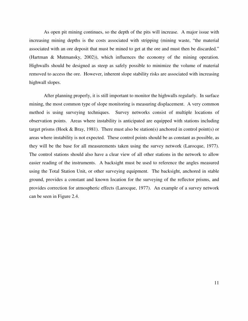
After planning properly, it is still important to monitor the highwalls regularly. In surface

mining, the most common type of slope monitoring is measuring displacement. A very common

method is using surveying techniques. Survey networks consist of multiple locations of

observation points. Areas where instability is anticipated are equipped with stations including

target prisms (Hoek & Bray, 1981). There must also be station(s) anchored in control point(s) or

areas where instability is not expected. These control points should be as constant as possible, as

they will be the base for all measurements taken using the survey network (Larocque, 1977).

The control stations should also have a clear view of all other stations in the network to allow

easier reading of the instruments. A backsight must be used to reference the angles measured

using the Total Station Unit, or other surveying equipment. The backsight, anchored in stable

ground, provides a constant and known location for the surveying of the reflector prisms, and

provides correction for atmospheric effects (Larocque, 1977). An example of a survey network

can be seen in Figure 2.4.

12

Figure 2.4: Example survey network

The angles and distances from the control station to each station of interest in the network

are measured on a regular basis to establish a history of movement on the slope. When/if

changes occur in the readings, the operator knows that movement has occurred and further

exploration of the cause of this movement is necessary. Errors such as dust, haze, extreme

temperatures, equipment deterioration and/or malfunction, and human error can have an effect on

the accuracy of the readings, but repeated measurements often minimize these factors.

Another method of stability monitoring is mapping tension cracks. The formation of

cracks is a somewhat apparent sign of instability in a slope. “Measuring and monitoring the

changes in crack width and direction of propagation is required to establish the extent of the

unstable area.” (Girard, Mayerle, & McHugh, 2006) One downfall to monitoring cracks is that

the rock has already shifted: cracking of the rock can loosen the entire area which has the

potential to weaken the ground, making measurements inaccurate. Another issue with tension

crack monitoring is the reality that the cracks seen on the surface may not accurately reflect the

extent and seriousness of the potential failure. This can be one of the more dangerous methods

of monitoring as well, as the operator who is measuring the cracks must enter a known instability

area, placing himself/herself at possible risk.

13

Wire extensometers are simple systems which have capabilities of alerting nearby

personnel in case of increased failure probability. The simple system has more than one

configuration. One of these setups consists of a wire anchored in the questionable area, which

runs over a pulley anchored in stable rock. The wire suspends a weight on the stable end, which

moves up or down along with the movement of the unstable rock. These wire extensometers can

be fitted with triggering mechanisms to alert nearby miners if a significant amount of

displacement occurs, although it is not common practice to do so. A sample setup of a wire

extensometer can be seen in Figure 2.5 below (after Girard, Mayerle, & McHugh, 2006).

Figure 2.5: Extensometer setup (after Girard, Mayerle, & McHugh, 2006)

One problem with wire extensometers is sag in the wire. The length of wire should be

limited to minimize the effects of sag. The counter weight is also matched to the type and length

of wire. Another setup of extensometer use involves anchoring two steel stakes into the host

rock, one on each side of the fracture in question. An invar tape extensometer is then fitted to

the stakes, and the displacement can be monitored. As daily displacement increases, less precise

tape equipment with a greater displacement range can be substituted (Larocque, 1977).

Inclinometers are also used to monitor the stability of highwalls in open pit mines.

Inclinometers (also known as tiltmeters) measure the inclination of an object with respect to

gravity. As seen in Figure 2.6 (after Girard J. M., 2006), the inclinometers give the operator an

estimate of how the rock is moving beneath the surface. The angles displayed on each

14

inclinometer can be combined to give a cross-section of the borehole they are monitoring, and

thus estimating the movement of the bench. In Figure 2.6 multiple sensors are displayed,

however to save money, the operator can use one inclinometer, which will decrease accuracy and

resolution in data. A single inclinometer can also be used in alliance with a track laid along the

walls of the borehole to allow the inclinometer to travel vertically and measure the inclination of

the entire borehole.

Figure 2.6: Monitoring slope stability with inclinometers (after Girard J. M., 2006)

Microseismic monitoring is used in open pit mines located in seismically active areas.

Here, microseismic monitoring can help warn operators of possible slope failure by detecting

seismically active zones which can cause rockbursts and earthquakes (Sjöberg, 1996). Seismic

events underground, either caused by a controlled event (explosion, hammer strike, etc.) or

microseismic events, can be examined to find areas of high stress in the earth. This procedure is

explained further in the subsurface section.

15

2.2.2- Monitoring at Underground Mines

The stripping ratio is often too great to economically mine using open pit methods. In

cases such as these, as well as in certain types of ore body formations, underground mining is

utilized to access the mineral deposit. Underground mining is more expensive than surface

mining, production is slower, and the cost of mining is higher (Hartman & Mutmansky, 2002).

In terms of ore production, subsurface mining extracts less than 5% of metals and nonmetals, and

since 1995, approximately 35% of US coal. However, the United States depends heavily on

underground mining for most of its supply of potash, lead, trona, zinc, molybdenum, salt, and

silver. (MSHA, 2007)

Surveying is used heavily in underground mines, and when performed properly, can be of

great use in mapping the mines progress as well as directing further production movement.

However, surveying, is not a major source of monitoring in underground mines, as it is time

consuming and can hinder progress of the production team. Surveying for monitoring slope

stability in surface mines can mostly be accomplished by setting up equipment at two or three

positions at the very minimum, while in underground mining, hundreds of points would be

needed.

The use of borehole extensometers is fairly common in underground measurements.

Borehole extensometers measure rock deformation parallel to the borehole and can only

withstand very small shear displacements normal to the borehole (CSMRS, 2006). If shear

displacements exceed the limits of the extensometer, the equipment becomes useless. The

system consists of a rod or wire (or multiple rods or wires) extending between the reference head

gauge and the anchor point. The instrument is grouted in the borehole leaving the reference head

on the rock surface. Figure 2.7 shows a typical borehole extensometer (after CSMRS, 2006).

Borehole inclinometers, also used for subsurface measurements, assess the angular

deflection of the borehole. They can be used to locate a failure surface in a sloped area that is

moving. Inclinometers are not the easiest equipment to monitor routinely, but can be very useful

in finding hazardous areas.

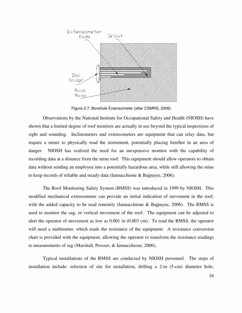
Figure 2.7: Borehole Extensometer

Observations by the National Institute for Occupational Safety and Health (NIOSH) have

shown that a limited degree of roof monitors are actually in use beyond the typical inspections of

sight and sounding. Inclinometers and extensometers are equipment that can relay data, but

require a miner to physically read the instrument, potentially placing him/her in an area of

danger. NIOSH has realized the need for an inexpensive monitor with the capability of

recording data at a distance from the mine roof. This equipment should allow operators to obtain

data without sending an employee into a potentially hazardous area, wh

to keep records of reliable and steady data

The Roof Monitoring Safety System (RMSS) was introduced in 1999 by NIOSH. This

modified mechanical extensometer can provide an initial indication of movement in the roof,

with the added capacity to be read remotely

used to monitor the sag, or vertical movement of the roof. The equipment can be adjusted to

alert the operator of movement as low as 0.001 in (0.003 cm). To read the RMSS, the operator

will need a multimeter, which reads the resista

chart is provided with the equipment, allowing the operator to transform the resistance readings

to measurements of sag (Marshall, Prosser, & Iannacchione, 2006)

Typical installations of the RMSS are conducted by NIOSH personnel. The steps of

installation include: selection of site for installation, drilling a 2

: Borehole Extensometer (after CSMRS, 2006)


of roof monitors are actually in use beyond the typical inspections of





data without sending an employee into a potentially hazardous area, while still allowing the mine

to keep records of reliable and steady data (Iannacchione & Bajpayee, 2006).

Safety System (RMSS) was introduced in 1999 by NIOSH. This


with the added capacity to be read remotely (Iannacchione & Bajpayee, 2006)



will need a multimeter, which reads the resistance of the equipment. A resistance conversion


(Marshall, Prosser, & Iannacchione, 2006).

ions of the RMSS are conducted by NIOSH personnel. The steps of

installation include: selection of site for installation, drilling a 2-in (5-cm) diameter hole;

16


of roof monitors are actually in use beyond the typical inspections of





ile still allowing the mine

Safety System (RMSS) was introduced in 1999 by NIOSH. This


2006). The RMSS is



nce of the equipment. A resistance conversion


ions of the RMSS are conducted by NIOSH personnel. The steps of

cm) diameter hole;

17

typically about 13 ft (3.9 m) into the roof, inserting the RMSS in the hole and attaching and

extending the cable along the roof and down the rib (Prosser, Marshall, Tadolini, &

Iannacchione, 2006).

Microseismic monitoring experience has shown that there is some correlation between

measurable rock noise and slope movement, but quantitative criteria are still lacking (Sjöberg,

1996). Even though the technical equipment needed for microseismic monitoring is currently

available, microseismic monitoring is not completely reliable: setbacks include filtering out the

noise from mining equipment and correcting arrival times for the actual length of travel for the

wave. Research and experimentation is being performed to help solidify the use of microseismic

monitoring in underground mining. In “Time-Lapse Tomography of A Longwall Panel: A

Comparison of Location Schemes”, by Kramer Luxbacher, the process of using microseismic

events to map out areas of high and low stress underground is described. As the P-waves travel

through the earth, they travel through many layers of rock, as well as many areas of differing

stress. Assuming homogenous rock content, the speed of the P-waves can be related to the

stresses in different areas of the rock mass, and with an array of sensors, a 3-dimensional

diagram, as well as 2-dimensional maps can be created mapping high and low stress areas. An

example of this method is seen in Figure 2.8 below, shows the inferred stresses on a longwall

face while the shear is operating (Luxbacher, 2007). The higher velocities are represented by

darker shades.

Figure 2.8

In a different case study, 15 geophones were used to study the microseismic events in an

underground limestone mine, where 2 distinct roof falls were observed. Over 700 microseismic

emissions were collected, and analyzed manually. After the occurrence of

could be seen that within 48 hours of first signs of roof failure, a large increase in filtered seismic

activity was present. In general, monitoring microseismic activity has potential to locate future

roof fall events, although determining the exact timing of these event is much more difficult and

may prove to be beyond the capabilities of the technology

2006).

2.3- Wireless Instruments

As the primary goal of this project is to study, design, and test wireless tiltmeters, it is

important to have an understanding of wireless technology. This section will give a brief history

of wireless technology, and describe current wireless products.

8: Plan view velocity tomograms at seam level



emissions were collected, and analyzed manually. After the occurrence of both roof falls, it



mining the exact timing of these event is much more difficult and

may prove to be beyond the capabilities of the technology (Iannacchione, Batchler, & Marshall,

this project is to study, design, and test wireless tiltmeters, it is


of wireless technology, and describe current wireless products.

18



both roof falls, it



mining the exact timing of these event is much more difficult and

(Iannacchione, Batchler, & Marshall,

this project is to study, design, and test wireless tiltmeters, it is


19

2.3.1- History of Wireless Technology

‘Communication without the use of wires other than an antenna’ is a fair definition of

wireless technology. This definition is shared by the radio. It should be known that the wireless

technology known and loved today has spawned from its ancestor, the radio (Dubendorf, 2003).

Guglielmo Marconi was one of the first individuals to develop commercial workable

radio communication, purportedly sending and receiving his first radio signal in Italy in 1895. In

early 1896, Marconi journeyed from Italy to England to demonstrate to the British telegraph

authorities his developments in operational wireless telegraphs. With the help of W. H. Preece, a

British electrical engineer, radio signals were transmitted wirelessly over a distance of 1.75 miles

in July 1896. Less than one year later, the distance had been more than quadrupled to 8 miles,

between Lavernock Point and Brean Down England (Dubendorf, 2003).

Though America was not among the first to realize the potential of wireless technology,

US scholars soon realized the commercial possibilities of the European technologies. In

September 1899, during the International Yacht Races held off of New York harbor, reports were

transmitted intermittently via radio devices by Marconi: the steamer Ponce was equipped with

radio devices and two receiving stations were equipped. Though this demonstration was not

very successful, it brought interest in the still new wireless technology to the United States.

Perhaps one of the greatest events of early radio was the reception by Dr. Marconi at St.

John’s, Newfoundland, of a transmitted test signal from his English station. This became known

as the famous letter “S”, which was successfully transmitted from England to Newfoundland on

December 11, 1901 (Dubendorf, 2003).

With the introduction of “Packet Data”, information was able to be sent wirelessly more

efficiently than before.

The transmission range is influenced by the power of the transmitter and the type and

location of the antenna. The length of the antenna and the frequency transmitted also play a

factor in the transmission range.

20

Voice transmission was accomplished in the 1920s, but the technology needed for such

equipment as wireless telephones or pagers was not readily available for public use. It was not

until the 1980s that the technology was perfected to the point that they became widely available

as consumer products (Dubendorf, 2003).

2.3.2- Current Wireless Technology

Many companies produce instruments that take physical measurements and transmit data

wirelessly. These instruments can potentially monitor any physical occurrence and transmit

digital data wirelessly to a receiver. Properties including (but not limited to) acoustic levels,

vibration, inclination, humidity, temperature, acceleration, pressure changes, and light exposure

can all be monitored. Wireless devices can be designed with event counters to record and

transmit the patterns and frequencies of set trigger mechanisms. Though the wireless

transmitting range is limited by the antenna type and size, the ability to transmit over long

distances is possible by using multiple relay stations, or even multiple sensors with the ability to

mesh together and transmit data to a single (or multiple) station. More powerful antennas can

also be used to increase the transmitting distance and reliability.

Wireless, micro electrical mechanical systems (MEMS) have proven to be useful in

monitoring the integrity of many civil structures. Philadelphia, PA is connected with Camden,

NJ, via the Ben Franklin Bridge. This 1927 suspension bridge, which supports seven lanes of

traffic, used to be monitored with wired instruments, but has recently changed to a MicroStrain

wireless sensor system. When using the wireless sensors, the engineers in charge observed an

increased ease and speed of installation. They also found that when switching to the new

MicroStrain system, they reduced the need for cable and its protection, realized a lower overall

system cost, and reduced pre-mature equipment repairs (MicroStrain, 2007).

Civil engineering is not the only industry to utilize the wireless inclinometers. In

November, 2006, a MicroStrain micro-sensor was successfully implanted in an artificial knee

replacement. This new “smart knee” has the ability to report digital, 3 dimensional torque and

force data back to computers. The sensor provides information on twisting, bending,

21

compressive and shearing loads across the human knee. These transmissions not only help

doctors monitor the stability of the knee replacement, they also help them better understand how

the human knee operates (MicroStrain, 2007).

The automotive industry is able to use wireless inclinometers custom designed for the

needs of automobile testing and qualification. Crossbow offers a complete inertial reference

system designed to allow automobile manufacturers and examiners to measure and analyze a

vehicle dynamic response. Tri-axial inclinometers coupled with accelerometers are used to

measure the pitch, roll, and yaw of automobiles as well as their respective dynamic information:

angles, rates, and accelerations (Crossbow, 2007).

Though traditional monitoring instruments have been used in mining for years to monitor

the stability of surrounding rock bodies, wireless technology is not yet widely accepted.

Wireless monitoring technology has benefits and setbacks when compared to traditional

scheduled monitoring.

One benefit of wireless instrumentation is the capability of real-time monitoring. When

using the traditional scheduled monitoring a quantity or quality is monitored at a scheduled time.

The reliability of the data depends greatly on the sampling rate, the amount of samples per given

unit of time. Some traditional instruments have the capability of measuring in real-time, but

many do not. One problem with scheduled monitoring is the consequences of an event occurring

between scheduled recordings. If a physical measurement changes between readings, the

operator has no knowledge about it until the next scheduled monitoring session. With real-time

monitoring, the status of a quantitative variable can be measured continuously. Recorded data

can also be viewed by the operator so that after a significant event, much more accurate time can

be delegated to changes in the measurement(s); which could allow the operator to determine

what actually caused the event in question. Graphs of measurement history are readily available

to any user with access to the recorded data, so trends in the data can be analyzed. The data can

be transmitted via the Internet to allow operators to view the status of monitored physical

measurements at any time, from any place, simply requiring an Internet connection (Accsense,

2007).

22

Another benefit of real-time monitoring is the ability to set up alarms when monitored

levels are exceeded. Triggers can be set up to alert staff via email and/or voicemail alarms if a

monitoring device records an extreme or unexpected measurement (Accsense, 2007). Also, the

instruments continue to monitor, even when the work crew is off duty. Information from the

sensors has the capability of being posted on the Internet for access on nights, weekends, and

holidays when no-one else is even in the vicinity of the sensor. This allows the operator to be

constantly alert of the status of their project.

An obvious benefit of wireless instrumentation is the lack of wiring costs. Wired

instruments spaced in larger areas require vast amounts of cables. With the rising costs of

precious metal commodities, the cost of cable will expectedly continue to increase. Wireless

instruments have no need for these expensive wires, so using wireless technology could save the

operator on costs.

Setbacks are also apparent in current wireless monitoring devices. The transmitting

range of most devices is not extremely impressive. Generally the upper limit of wireless

transmitting is around 250 ft, but the distance is dependent on line of sight. There are

transceivers that will operate as far as one mile from its receiving antenna, but distances like

these are not incredibly common. As with any wireless devices, barriers and objects between the

transmitter and the receiver often interfere with the quality and reliability of the transmission.

These setbacks present a real issue to be considered in mining. Surface mining often

takes place on a large scale, so distances between highwalls and structures is generally greater

than 250 ft. One of the more common types of subsurface mining is room and pillar mining,

which incorporates support pillars of the host material. The wireless signals used in the devices

in question will not penetrate these roof supporting barriers. To resolve both issues in the

described situations, a network of multiple sensors would need to be used, to allow multiple

relay stations before the signals are finally transmitted to a central data storage device.

Another issue comes with the power source of the device. Though most instruments can

be powered by an external power source, the instrument would need to be battery powered in

23

situations that require truly wireless monitoring. The life of the batteries used in many sensors is

not much more than 6 months (varies with different sampling rates and other settings within

individual sensors), which would require the operator to replace batteries at least twice a year, if

not more. This could cause minute disruptions in the work cycle unless planned into the

schedule properly. To reduce the probability of sudden sensor loss due to battery failure, alarms

on the sensors can allow the operator advance notice of lowered supply voltage, and provide

ample time to replace the batteries.

Mining conditions are often very rugged, and the instruments available today may not be

ready for the mining environment. In underground coal mines, the ever present coal dust and

rock dust may interfere with the instrumentation in the device. In surface mining, the possibility

of minor rock falls occurring above a sensor on a highwall exists: even though fist sized rocks

may only fall short distances, the momentum generated by the falling material could be enough

to damage current wireless instruments. The ever presence of water could also provide

unwanted short circuiting in equipment.

24

CHAPTER 3: PRELIMINARY DATA COLLECTION

The Accsense A1-01a sensor pod was tested for reliability (continuity of wireless

transmissions), ease of use, and sensitivity. The following chapter discusses the procedure and

some results of preliminary testing of already existing equipment, as well as testing the

accelerometer chosen for use in the circuit board. For more information on the circuit board,

refer to Chapter 4: Designing a Wireless Tiltmeter.

3.1- Accsense Wireless Systems

The Accsense A1-01A sensor pod is designed for general measurements. Within the pod

casing, there are several different internal sensors, as well as an exterior terminal for wiring

additional instruments to the pod. The pods have the ability of storing up to 255 data points

before transmitting, and have a range of approximately 260 ft (80 m). The internal sensors

include equipment to measure ambient temperature, vibration, humidity, acoustic level, and

ambient light (Accsense, 2007).

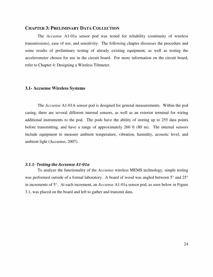
3.1.1- Testing the Accsense A1-01a

To analyze the functionality of the Accsense wireless MEMS technology, simple testing

was performed outside of a formal laboratory. A board of wood was angled between 5° and 25°

in increments of 5°. At each increment, an Accsense A1-01a sensor pod, as seen below in Figure

3.1, was placed on the board and left to gather and transmit data.

25

Figure 3.1: Accsense A1-01a Sensor Pod

After sufficient time, the sensor was rotated 90° on the plank to test the sensitivity of the

internal accelerometers for each axis, positive and negative, X- and Y-. As the pod was rotated,

any measurements taken during the time of rotation were ignored. As mentioned before, the

pods were placed on a plank of varying angle from the horizontal plane. At each angle, the

sensors were tested with four rotations, denoted as antenna NE, SE, SW, and NW for continuity.

These rotations would allow testing of both the X- and Y- axes, as well as positive and negative

angles for each axis. The headings given as descriptions to the antenna arrangement have no

relation to true North, but were simply a descriptor to help repeat the same measurements for

each angle. As the sensor pod was rotated, or the angle of inclination was altered, the time of

day was recorded to aid in data analysis.

The Accsense A1-01a sensor pods operate by transmitting a wireless voltage reading to a

“gateway”, which can be purchased through Accsense (Accsense, 2007). The gateway used for

the purpose of this experiment is the Accsense B1-01, as seen below in Figure 3.2.

26

Figure 3.2: Accsense B1-01 Gateway

The gateway is connected to the Internet via an Ethernet cable on its rear panel (same

panel as antenna as seen above in Figure 3.2). With this Ethernet connection, the Accsense B1-

01 has the ability to post real-time data on the Accsense website (Accsense, 2007). With a valid

username and password, an operator has the ability to check on his active sensors from anywhere

in the world, provided a PC with Internet connectivity.

The Accsense website automatically takes the data transmitted from the gateway and

forms a number of visual aids for viewing the data. The website allows the operator to view data

on a time-based level. Charts are automatically loaded for the last 4 hours of recorded

measurements, but the duration of data points can be changed easily. Hours, days, weeks, even

months of data can be viewed using the built in scatter plots. The actual data numbers can also

be viewed on a separate tab, as well as saved and downloaded onto your own PC. The

minimum, maximum, average, median, and standard deviation for the selected duration of data

points are also displayed on the same page, making a quick assessment of the data. If a further

27

analysis of the data is required, as was the case in this project, the data values can be downloaded

and viewed in Microsoft Excel.

3.1.2- Accsense Results

After analyzing the data collected by the Accsense A1-01a sensor pod, it was decided the

sensitivity of the included accelerometer was not sufficient for the purpose of this project.

Desired sensitivity was around 0.5°, and the Accsense sensor pods were only displaying obvious

visual and statistical changes of between 1 and 2 degrees. The standard deviation of the readings

were simply too high for accurate angle measurements.

A major problem with the design of the sensor pod was the output reading was a sum of

all axis measurements. The resulting voltage could represent a variety of angles given the same

output. In a perfect situation where an angle was to change on one axis, as well as change

equally negative on the other, no voltage difference would be detected. This misrepresentation

of angle was observed a number of times during the testing stages of the Accsense A1-01a.

Figure 3.3 below shows an example of the readings from the sensor pod and illustrates how two

angles can have the same (or similar) outputs. As visible in the chart, the 5° and 10° readings are

very similar, where the 15°, 20°, and 25° are distinctively different, even varying what could be

estimated as linearly. Also visible in Figure 3.3 is the level of noise, which was somewhat

significant. Because each measurement varied so heavily, a change may not be as easily noticed.

Data tables were compiled containing measurements at each inclination. Tables

containing the relation of alignment, (NE, SE, etc.) were also constructed from the data, however

this data was not used; ergo it was not included in the appendixes. Figures were created to

visually display the relationships of the four antenna bearings at each angle, as well as comparing

the angular readings for each accelerometer alignment. The data tables can be found in Table

A.1 through Table A.4 in Appendix A.

28

Figure 3.3: Accsense A1-01a output voltage

3.2- Other Wireless Systems

Crossbow and MicroStrain, among other companies, manufacture wireless MEMS

sensors that could feasibly be used in the mining environment; however these products were not

tested for this project. Crossbow sensors, as seen below in Figure 3.4, were available for use, but

because of software installation issues, they were not able to be tested. MicroStrain sensors were

not available for testing, and the budget for this project did not allow for their purchase.

Therefore an analysis of the MicroStrain sensors could not be performed.

Figure 3.4: Crossbow Sensors

16

16.2

16.4

16.6

16.8

17

17.2

17.4

1 5 9 13 17 21 25 29 33 37 41 45 49 53 57 61 65 69 73 77

Se

nso

r O

utp

ut

(V)

Measurement Number

NE Alignment

5°

10°

15°

20°

25°

29

3.3- MEMSIC Accelerometers

Aside from testing the already existing equipment, individual accelerometers were tested

for design of a new product. The MEMSIC accelerometers tested for the purpose of this project

were ordered online from the MEMSIC website. The MXR6999M accelerometer was chosen

because of its posted sensitivity and other product ratings found online. The MXR6999M is a

thermal accelerometer with 2 axes of measurements and a claimed sensitivity of 1000 mV/g. A

sensitivity of 1000 mV/g simply means that for each g force, there are 1000 increments of 1 mV.

For most accelerometers, 1 g is seen when 1 of the axes is aligned perpendicular to the horizontal

plane. Therefore, a sensitivity of 1000 mV/g claims to have 1000 digital steps from horizontal to

vertical, or 90°. If assumed linear, each increment would represent a change of 0.09° in theory.

The change in voltage, in reality, is not linear to the change in tilt. The accelerometer is

most sensitive to changes in tilt when the accelerometer is perpendicular to the force of gravity

and least sensitive to changes in tilt when the accelerometer is parallel to the force of gravity. In

other words, when one axis of the accelerometer is vertical, changes in inclination are less

obvious. The MXR6999M datasheet includes a table of approximate voltage readings for axis

orientations. The table found on the datasheet has been recreated below in Table 3.1 (after

MEMSIC, 2008).

Table 3.1: Changes in Tilt for X- and Y- Axes X-Axis

Orientation to Earth's Surface (deg.)

X-Axis Y-Axis

X Output (g)

Change per deg.

of tilt (mg)

Y Output

(g)

Change per deg.

of tilt (mg)

90 1.000 0.15 0.000 17.45 85 0.996 1.37 0.087 17.37 80 0.985 2.88 0.174 17.16 70 0.940 5.86 0.342 16.35 60 0.866 8.69 0.500 15.04 45 0.707 12.23 0.707 12.23 30 0.500 15.04 0.866 8.69 20 0.342 16.35 0.940 5.86 10 0.174 17.16 0.985 2.88 5 0.087 17.37 0.996 1.37 0 0.000 17.45 1.000 0.15

30

3.3.1- Testing the MEMSIC MXR6999M

The MXR6999M was tested using a simple experiment consisting of a simple straight

board and a moving fulcrum. The angle of the board was changed in half degree increments by

raising the adjacent leg of the triangle to predetermined lengths. Simple trigonometric

calculations allowed the vertical leg to be measured, keeping a constant hypotenuse, as seen

below in Figure 3.5.

Figure 3.5: Testing the MXR6999M

Using the equation: � �� = �� a given angle (α) could be measured by keeping a

constant hypotenuse (C) (or length of the board), and changing the vertical leg (B) as seen above

in Figure 3.5.

The MXR6999M Accelerometers were soldered to special evaluation boards, which were

purchased from the MEMSIC website. Each evaluation board (here-in referred to as EB) had a

solder pad for each respective pin on the MXR6999M. These solder pads connected the pins of

the accelerometer to easier accessible pads where wires were soldered for the purpose of

analysis. The accelerometers were hand soldered to the EB’s, and tested using the simple board

experiment described above. An image of the EB and accelerometer, with attached wires, can be

seen below in Figure 3.6.

Base (A)

Hypotenuse = Length of Board (Constant)

(C) Changing Vertical Leg. (B)

α

31

Figure 3.6: MXR6999M and Evaluation Board

As mentioned in the MXR6999M datasheet, the accelerometer has an arrow as a logo,

indicating the negative X- Axis. The positive X- Axis therefore is in the opposite direction of the

MEMSIC logo, and the Y- Axis follows the right hand rule (MEMSIC, 2008). The X- and Y-

Axis are labeled above in Figure 3.6 for visual reference. Refer to the MXR6999M datasheet for

a Pin Diagram and Pin Spacing figures (MEMSIC, 2008).

To test the MEMSIC accelerometers, an experiment was designed so that only one axis

would change at a time. This experiment consisted of a plank of stiff wood, with one end

anchored. The other end was lowered and raised to attain angles of 0°, 0.5°, 1.0°, 1.5°, 2.0°,

2.5°, 3.0°, 4.0°, 5.0°, 10.0°, 15.0°, and 20.0° from horizontal. The MEMSIC accelerometer is

capable of reading angles at varying frequencies, so for the purpose of consistency, it was

necessary to find the optimal operating frequency for both axes.

By testing the mean and standard deviation of the readings at 0° using frequencies of 1

Hz, 10 Hz, 50 Hz, 100 Hz, 500 Hz, 1,000 Hz, 5,000 Hz, and 10,000 Hz, it was determined that

the optimal operating frequency was 100 Hz. The data table containing all 100 samples for all

frequencies can be found in Table A.5 and Table A.6 in Appendix A. The charts displaying the

mean and standard deviation for an inclination of 0° and the aforementioned frequencies can be

seen below in Figure 3.7 and Figure 3.8 (X- and Y- axes respectively). This experiment was

only performed once for each frequency: repeadability was assumed. As is visible in the figures

below, 100 Hz is a fair frequency for both the X- and the Y-axes: the standard deviation (as seen

in the error bars) for both axes is significantly lower at this sample rate. With a lower standard

X- Out

Y- Out

Voltage (3V)

Ground

+Y

+X

32

deviation, the sensitivity of the accelerometer is increased, allowing the user to determine

smaller changes in inclination.

Figure 3.7: X-axis frequency test with ±2 standard deviation error bars

Figure 3.8: Y-axis frequency test with ±2 standard deviation error bars

1.345

1.350

1.355

1.360

1.365

1.370

1.375

1 10 100 1000 10000

Acc

ele

rom

ete

r O

utp

ut

(V)

Sample Rate (Hz)

X- Axis Frequency Test

1.335

1.340

1.345

1.350

1.355

1.360

1.365

1.370

1 10 100 1000 10000

Acc

ele

rom

ete

r O

utp

ut

((V

)

Sample Rate (Hz)

Y- Axis Frequency Test

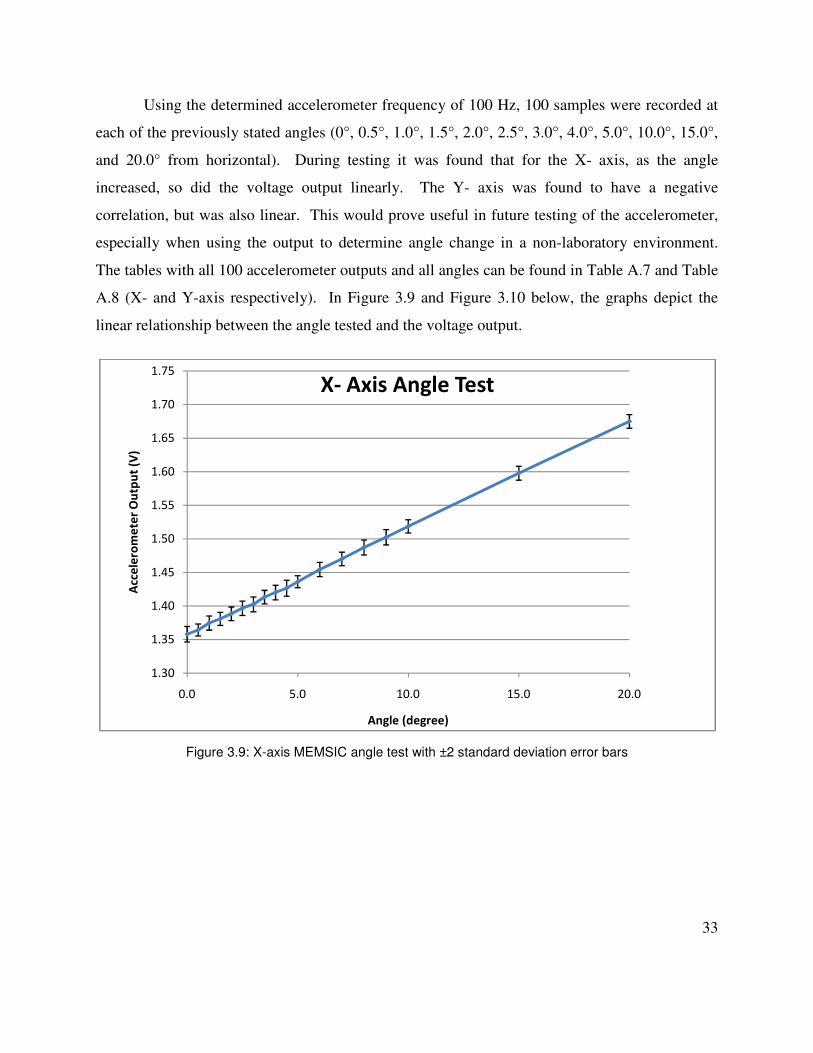
33

Using the determined accelerometer frequency of 100 Hz, 100 samples were recorded at

each of the previously stated angles (0°, 0.5°, 1.0°, 1.5°, 2.0°, 2.5°, 3.0°, 4.0°, 5.0°, 10.0°, 15.0°,

and 20.0° from horizontal). During testing it was found that for the X- axis, as the angle

increased, so did the voltage output linearly. The Y- axis was found to have a negative

correlation, but was also linear. This would prove useful in future testing of the accelerometer,

especially when using the output to determine angle change in a non-laboratory environment.

The tables with all 100 accelerometer outputs and all angles can be found in Table A.7 and Table

A.8 (X- and Y-axis respectively). In Figure 3.9 and Figure 3.10 below, the graphs depict the

linear relationship between the angle tested and the voltage output.

Figure 3.9: X-axis MEMSIC angle test with ±2 standard deviation error bars

1.30

1.35

1.40

1.45

1.50

1.55

1.60

1.65

1.70

1.75

0.0 5.0 10.0 15.0 20.0

Acc

ele

rom

ete

r O

utp

ut

(V)

Angle (degree)

X- Axis Angle Test

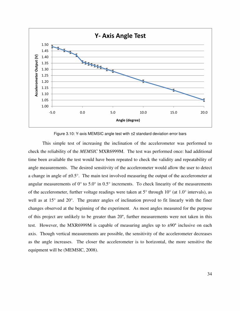
34

Figure 3.10: Y-axis MEMSIC angle test with ±2 standard deviation error bars

This simple test of increasing the inclination of the accelerometer was performed to

check the reliability of the MEMSIC MXR6999M. The test was performed once: had additional

time been available the test would have been repeated to check the validity and repeatability of

angle measurements. The desired sensitivity of the accelerometer would allow the user to detect

a change in angle of ±0.5°. The main test involved measuring the output of the accelerometer at

angular measurements of 0° to 5.0° in 0.5° increments. To check linearity of the measurements

of the accelerometer, further voltage readings were taken at 5° through 10° (at 1.0° intervals), as

well as at 15° and 20°. The greater angles of inclination proved to fit linearly with the finer

changes observed at the beginning of the experiment. As most angles measured for the purpose

of this project are unlikely to be greater than 20°, further measurements were not taken in this

test. However, the MXR6999M is capable of measuring angles up to ±90° inclusive on each

axis. Though vertical measurements are possible, the sensitivity of the accelerometer decreases

as the angle increases. The closer the accelerometer is to horizontal, the more sensitive the

equipment will be (MEMSIC, 2008).

1.00

1.05

1.10

1.15

1.20

1.25

1.30

1.35

1.40

1.45

1.50

-5.0 0.0 5.0 10.0 15.0 20.0

Acc

ele

rom

ete

r O

utp

ut

(V)

Angle (degree)

Y- Axis Angle Test

35

In addition to the aforementioned angles, the accelerometer was tested at negative angles

to ensure continuous linearity of voltage vs. inclination. As the negative angles were plotted

alongside the positive angles, a slight jump in voltage reading was encountered. This jump

remains unaccounted for; further research should be attempted before finalizing a design for

mass production. As seen in Figure 3.10, the slope of the linear correlation for the negative

angles was relatively the same as correlation in the positive data points.

As visible in Figure 3.9 and Figure 3.10, the standard deviation of the readings remained

somewhat constant. This is beneficial in serving the purpose of the accelerometer, for the user

can understand the error range of the equipment while reading the output data. With greater

standard deviation comes greater uncertainty of accuracy in measurement, so the relatively low

standard deviation found in this experiment are reassuring of the prospective success of the

MXR6999M accelerometer.

3.3.2- MEMSIC Results

Upon conclusion of the tests described in 3.3.1- Testing the MEMSIC MXR6999M, it

was found that within one standard deviation, a change of inclination of roughly 0.4° could be

detected. With this conclusion, the MXR6999M accelerometer was approved for use in the

design of the circuit board, as described in Chapter 4: Designing a Wireless Tiltmeter.

3. 4- Other Accelerometers

Aside from the MEMSIC MXR6999M, a number of other accelerometers produced by

Analog Devices were considered for use in the project design. The ADXL330 was a candidate

because it is a 3-axis accelerometer. 3 samples were provided by Analog Devices, but were not

tested due to the package of the accelerometer. The term package refers to the size, shape, pin

location, and pin spacing of the equipment. A specific connection port would have been needed

to test the ADXL330, and budgeting and timing for this project did not allow for such a

purchase. Also, the sensitivity of the ADXL330 was not sufficient. A mere 300mV/g would

most likely have not yielded the results desired for this project. (Analog Devices, 2008)

36

The ADXL103 was also provided by Analog Devices, but no evaluation boards (EB)

were provided with the accelerometer. Unfortunately, without an EB, the 5 ADXL103 units

provided as samples from Analog Devices could not be tested. The ADXL103 is a single axis

accelerometer, so even if an EB was available and the device was tested, it was not ideal for use

in this project. (Analog Devices, 2008)

Another product very similar to the ADXL103 is the ADXL203, which is a dual axis

accelerometer made by Analog Devices. The ADXL203 was not available for samples until late

in the project lifeline. Even though Analog Devices was kind enough to provide 5 ADXL203

units with already mounted on EB’s, the timing was unfortunate as the MEMSIC MXR6999M

had already been selected for use and ordered in quantity 10 for mounting on the circuit boards.

The ADXL203 is very similar to the MXR6999M in specifications. Both have sensitivities of

1000 mV/g, have similar voltage supply requirements, and are bi-axial accelerometers with

analog output. The package for the ADXL203 is also very similar to that of the MXR6999M;

meaning that some of the 8 pins on the accelerometer have the same designated function.

Voltage and ground pins are almost identical, even the X- and Y- axis output pins were the same

(Analog Devices, 2008)(MEMSIC, 2008). If the size of the accelerometer package, as well as

the exact distance between pins were identical, the ADXL203 could be substituted for the

MXR6999M on the circuit board design and the functionality of the sensor would most likely

remain intact.

37

CHAPTER 4: DESIGNING A WIRELESS TILTMETER

In an effort to tailor the instrument to the specific requirements of this project, it was

decided to design a new and unique device. To link the MXR6999M accelerometer with the

XBee wireless transceiver, a circuit board was needed. Refer to 4.1.1- Transceiver selection for

more on the XBee transceiver. Since circuit boards are not easily purchased for such a specific

task, especially in smaller quantities for prototype models, it was decided to construct a unique

circuit board for the purpose of this project using Eagle software.

4.1- Circuit Board Design

Eagle is a German made computer program allowing users to create circuit boards using

devices that exist in previously created “libraries” or conglomerations of user created

components. It is also possible to design new “parts”, or components, to suite the user’s specific

requirements. These devices are added and linked together in a schematic using Eagle. From

the schematic, a digital copy of a circuit board can be created. This digital blueprint of the

circuit board contains all the components of the project needed to make the entire board function

properly: the accelerometer, the transceiver, the processor, and all resistors, capacitors, diodes,

and transistors needed to make all the components function properly. These devices can be

moved, rotated, and connected together using Eagle, to create a compact and functional circuit

board. In the case of this project, almost all devices (resistors, capacitors, transistors,

transceivers, etc) existed in previously created libraries and could be accessed for use without

copyright infringement; the only device that needed to be designed from scratch on this program

was the connection for the accelerometer. (Bird, Eagle Software, 2007)

38

4.1.1- Transceiver selection

As this circuit board was desired primarily for wireless use, a transceiver would be the

key component in its design. For the purpose of this project, multiple transceiver manufacturing

companies were researched online, and Digi International’s XBee transceiver was selected.

A low cost ($21 each), low power (2.1 – 3.6V), mesh networking capable device, the

XBee transceiver was considered ideal for the purpose of this project. The XBee selected has an

indoor range of up to 133 ft (40 m) and an outdoor range of up to 400 ft (120 m). If this distance

is deemed too short, XBee PRO transceivers are available at $34 each, and have an indoor range

of up to 300 ft (100 m) and an outdoor range of up to 1 mile (1.6 km). For the purpose of this

project, the normal XBee transceiver was selected, as distances greater than 100 ft (30 m) were

not expected. (Digi International, 2008)

The XBee transceivers have a serial data rate of 1200 – 230,400 bps, which greatly

exceeds the data rate expected for this project. Multiple baud rates are supported by the

transceiver which would prove useful when programming, as described in 4.3- Programming the

Circuit Board. The XBee transceiver has capabilities for sleep mode, which was not used for this

project, but is recommended for further research and development of the tiltmeter. (Digi

International, 2008) The XBee transceiver can be seen below in Figure 4.1.

Figure 4.1: XBee Transceiver

Please refer to Figure 4.1 for scaling purposes of all images of circuit boards throughout

the remainder of this document. A Pin Diagram for the XBee can be found on the Digi

International website (Digi International, 2008).

39

4.1.2- Prototype Circuit Board

To properly design the circuit board, an initial prototype board was designed for analytic

purposes. Using Eagle, the circuit board was laid out and organized for ideal analysis in the

testing stages, with solder test points (to test voltage readings) for important connections, LED

diodes for visual confirmation of sending and receiving data, and switches for testing different

XBee transceiver settings. Test points would also prove useful for connecting additional

components if errors in the planning of the board were made. These additions to the board

would not be necessary in a production model, but proved useful in the testing stages. This

initial prototype would be tested using a CR2032 cell battery, and after fine tuning of the

switches, observing the patterns of the diodes and test point indication, modifications to the

schematic and board would be made. The schematic and board for this initial prototype model

can be seen in Figure 4.2 and Figure 4.3 respectively.

40

Figure 4.2: Initial Prototype Schematic

41

The blue rectangle that contours the border of the board is known as a ground plane,

which will fill all empty space on the bottom of the board when created. The ground plane

allows for easier routing as well as provides a more consistent and better quality ground to all

components.

Figure 4.3: Initial Prototype Board

After designing the prototype circuit board in Eagle, a group of different layer files were

generated to be sent to a circuit board manufacturing company. Seven layers including drill

holes, top and bottom copper connections, top and bottom solder mask, and top and bottom silk-

screen were created and uploaded to Advanced Circuits (Advanced Circuits, 2008). Advanced

Circuits took the provided layers and manufactured the circuit board represented in Figure 4.3.

Once the circuit board was completed in Eagle, additional components were necessary

for its operation. Capacitors, resistors, transistors, diodes, and other electronic components were

ordered from Digi-Key online (Digi-Key, 2008). Some of the parts were available as samples

from other manufacturing companies. Texas Instruments provided samples of the MAX3232,

Microchip provided samples of the PIC18F6722, and Mill-Max provided samples of headers for

the XBee transceivers (Texas Instruments, 2008)(Microchip, 2008)(Mill-Max, 2008). Also, the

accelerometer used in this design came from MEMSIC, and the XBee transceiver was ordered

from Digi International, formerly MaxStream (MEMSIC, 2008)(Digi International, 2008). A list

42

of all the necessary components for the prototype board, along with their product numbers and

company from which they were purchased or ordered can be found in Table C.1 in Appendix C.

Once all components arrived from their respective manufacturing companies, they

needed to be soldered to the circuit board. To accomplish this, the hot plate and solder syringe at

the Virginia Tech Unmanned Systems laboratory were used. A solder paste containing miniscule

spheres of solder in a liquid flux was applied using a syringe, to fasten all components to their

designated board locations. The board (with loosely attached components) was then placed upon

the hot plate to activate the solder in the flux, and permanently attach all components to the

board. A few minutes after placing the circuit board on the 235° F hot plate, the solder was fully

activated, and all surface mounted components were successfully attached. Additional soldering

was required for the “through hole” components. The necessary jumpers, headers, and serial

connectors were soldered to the board by hand, completing the process. (Bird, Virginia Tech

Unmanned Systems Laboratory, 2008) The result was a prototype board ready to be tested for

analysis. The prototype board, after soldering, can be seen below in Figure 4.4.

Figure 4.4: Physical Prototype Circuit Board

43

4.1.3- Revisions to the Circuit Board

After testing the prototype, changes were made to the schematic and board, and a new

board was ordered. This new board was also tested and further changes were made.

Unfortunately, an error was found in the board layout, and a third board was designed. Because

this third board was tested in a live mining environment, it was ordered in quantity five. For

more details on the testing of the final revision board, see Chapter 5: Multiple Tiltmeter Testing.

The schematic for the final board was slightly different than the prototype. The prototype

board had a total of 5 diodes, while the new board would only have two, one to illuminate when

data was sent, and one to illuminate when data was received. The prototype board also had

additional jumpers to test specific connections. These were thought to be useful when the board

was being designed, but were considered unnecessary after testing of the prototype. Another

difference between the prototype schematic and the test product schematic is the number of test

points. Test points can be useful, and are relatively small in size; however, during the prototype

testing, many existing test points were left untouched. Therefore, their existence on the board

was deemed unnecessary. Another change made to the schematic was the power supply. Instead

of using a single CR2032 cell battery, the board would be connected to a pair of 3V AA

batteries. This modification allowed a significant increase the battery life. The new schematic

for the revised circuit board can be seen below in Figure 4.5.

44

Figure 4.5: Final Revised Schematic

45

The new board was designed to be smaller and more ergonomic than the prototype board.

Experience gained when designing and testing the prototype board helped to dictate the preferred

placement of resistors, diodes, and other components. The overall size of the board was reduced

to match the dimensions of the twin AA battery housing, and allowed the battery housing to be

mounted on the reverse side of the board, gaining space for the rest of the components. The

designed board can be seen below in Figure 4.6.

Figure 4.6: Final Revised Board

This final board followed the same procedure of component population as did the

prototype board. Refer to 4.1.2- Prototype Circuit Board for details on the soldering process.

The soldered final revision of the circuit board can be seen below in Figure 4.7.

Figure 4.7: Physical Final Revised Circuit Board

46

4.2- Cost Analysis

To analyze the cost of each board, a program in Eagle, that allows the user to create a Bill

of Materials (BOM), was utilized. This BOM was joined with the component list from Digi-Key,

Digi-International, and MEMSIC to accomplish an estimate of the unit cost for the prototype

board as well as the final revised production board. Details for the cost analysis of both boards

can be found in the following sections.

4.2.1- Cost Analysis for the Prototype Board

A detailed BOM for the prototype board can be found in Table C.1 in Appendix C. The

contents of the prototype board’s BOM were slightly altered to properly analyze the cost of one

circuit board: the columns Description, Part #, and Company were excluded from the analysis,

while the preceding columns Part, Value, Device, and Package were included for recognition of

parts on the order forms.

Table C.3, as seen in Appendix C, was created to show the estimated cost of one unit of

each component required for the prototype circuit board. The prices listed in Table C.3 do not

include shipping costs, processing fees, sales tax, or any labor costs.

As seen in the final row of Table C.3, the total cost of the components on each prototype

board was $53.64. The cost of each blank board from Advanced Circuits was $33. Adding these

numbers yields a total of $86.64 for each prototype board.

47

4.2.2- Cost Analysis for the Revised Board

A detailed BOM for the revised board can be found in Table C.2 in Appendix C. The

contents of the revised board’s BOM were slightly altered to properly analyze the cost of one

circuit board: the columns Description, Part #, and Company were excluded from the analysis,

while the preceding columns Part, Value, Device, and Package were included for recognition of

parts on the order forms.

Table C.4, found in Appendix C, was created to display the estimated cost of one unit of

each component required for the final revised circuit board. As in Table C.3, the listed prices do

not include shipping costs, processing fees, sales tax, or any labor costs.

As seen in the final row of Table C.4, the total cost of the components on each revised

board was $52.32. The cost of each blank board from Advanced Circuits was $33. Adding these

numbers yields a total of $85.32 for each revised board. Although the difference in the cost of

each revised board and the cost of each prototype board is not significant, the reduction comes

from the changes made in Eagle as work on the project progressed.

When future boards are ordered, they will likely be ordered in larger quantities, resulting

in a reduction of the cost, significantly reducing the overall cost per unit. The components that

populate each board will also be ordered in mass quantity, further reducing the cost per

component. Also, with future boards, certain components would not be necessary, as described

in 7.1- Future Recommendations.

4.3- Programming the Circuit Board

Once the boards were designed, ordered, and soldered with the necessary components,

they needed to be tested. Before testing however, the blank processing units (PIC18F6722)

needed a program to guide the operation of all the components in a system to send wireless serial

data from one circuit board to another.

48

4.3.1- Background

As mentioned before, the processing unit for the designed circuit board is the

PIC18F6722 (here-in referred to as the PIC). The initials PIC represent a family of

microcontrollers manufactured mainly by Microchip Technology. The name PIC is an acronym

for “Programmable Intelligent Computer”. PIC’s are popular because of their wide availability

and their relatively low cost. There are many families of PIC’s, including the 16F, 18F, and

others. Each family has slightly different capabilities and packages (pin layouts and spacing).

The PIC18F6722 was selected as the processing unit in this design because of a recommendation

from a colleague, John P. Bird, who deals with these processors on a more regular basis (Bird,

Eagle Software, 2007). A Pin Diagram for the PIC18f6722 can be found on the Microchip

PIC18F8722 Family Data Sheet (Microchip, 2004).

When purchasing a PIC, the processor arrives devoid of code. The user must write the

codes or use already existing code to make the processor function to its intended functionality.

When the PICs and all other components were soldered to the circuit board, the first step was to

install a bootloader. This was done using a “logger” owned by the Virginia Tech Unmanned

Systems lab. Loading this bootloader onto the 5-pin serial port allowed any user to utilize a 3-

pin serial port to program the PIC. This is beneficial in many ways: without the use of the 3-pin

serial port, all commands would need to be written on the logger, one line at a time, and

programmed using this special equipment; by using a 3-pin serial port, any PC with standard

load software can write code to the PIC. (Bird, Virginia Tech Unmanned Systems Laboratory,

2008)

After loading the bootloader onto the PIC, a series of test codes were written, compiled

and loaded to the PIC before the final code was loaded for production use. The first step was

writing the code to be loaded. To accomplish this task, a program called PIC C Compiler

(Custom Computer Services, Inc., 2008) was used. This program allows the user to write the

code using the C programming language. The code must be compiled using PIC C Compiler’s

built in compiler to change the C code to hexadecimal (HEX) format, which is what the PIC

understands and can run. After the code was developed and compiled using PIC C Compiler, the

program Tiny PIC Bootloader was used to digitally write the code to the PIC. A description of

49

the procedure of the actual cycle of writing the code, compiling the code and then loading the

code to the PIC can be found in Appendix B on page 113.

4.3.2- Codes Used for Testing and Programming PIC

A simple code, “toggle”, was written to test the functionality of the PIC. The code

“toggle” can be found in the Appendix B-1. “Toggle” simply forces one pin of the 64 pins on

the PIC to turn on (showing a voltage of 3V) and then turn off to 0V after 2 seconds. This

process repeats so the user can measure the voltage on this pin to confirm the PIC is operating

properly. “Toggle” was only used on the first prototype board to test the connection settings; on

future boards this was not used, as the connection settings remained basically the same for the

PIC.

Once the PIC was determined to function properly, a second program was written to test

the serial functionality of the PIC. “Serial Test” was written to force the PIC to output a message

every second reading “TEST SERIAL”. This serial message was read by connecting the PC

used for this project to the “SERIAL” port on the prototype circuit board, and the “SERIAL-

PIC” port on the final revised board. “Serial Test” can be found in Appendix B-2.

After testing the serial functions of the PIC, it was decided to test the functionality of the

accelerometer with the PIC, as well as the PIC’s computational abilities. To accomplish both of

these tasks, the program “Test ADC” was written. The source code entitled “Test ADC” can be

found in Appendix B-3. “Test ADC” forced the PIC to read two pins connected to the

accelerometer’s X- and Y- axes, and sum a total of ten measurements, displaying a combination

of text and values over a serial output pin.

All of these programs could be tested using the serial ports on the circuit board, so a

simple homemade serial extension was used to read the output messages. The serial extension,

as seen below in Figure 4.8, was fabricated to connect pins 1, 2, and 3 on the circuit board

connecter directly to pins 2, 3, and 5 respectively on the serial port of a common PC. (Bird,

Virginia Tech Unmanned Systems Laboratory, 2008)

50

Figure 4.8: Serial Connector

This serial connector, which simply ties the sending, receiving, and ground pins to each

other, was used heavily in the testing of the prior codes. Unfortunately, it would prove useless

when testing the wireless capabilities of the circuit board. In order to test the Digi International

XBee transceiver (here-in referred to as the XBee), a separate device was needed, and was

purchased from Digi International.

4.3.3- Wireless Transmission

The XBee interface board XBIB-U-DEV, as seen below in Figure 4.9, connects a single

XBee unit to a USB-b port, which in turn connects to the USB-a port on a common PC.

Figure 4.9: XBIB Interface Board

USB-b Port

51

After installing the necessary drivers provided by representatives of Digi International,

the interface board operated exactly as the serial connector, with the exception of the COM port.

The serial connector used COM port 1, while the wireless interface board (XBIB) operated on

COM port 7. (Digi International, 2008)

Another important step was setting up an association between the XBee modules. This

was accomplished by using the program X-CTU which was downloaded from the Digi

International website with the assistance of a Digi International associate. For mesh network

designs, the sensors in the network need to be programmed as “Routers”. This term describes

their ability to send original data, as well as relay data received from other “Routers”. One

XBee, the XBee connected to the PC, needed to be programmed as a “Coordinator”. (Digi

International, 2008) The “Coordinator” does not send data, but rather receives all transmissions

and relays them to the serial program on the PC. It is recommended that the “Coordinator” XBee

is marked to differentiate it from the “Router” XBees, as there are no visual differences between

the two.

After setting up the wireless Coordinator on the XBee interface board, the next step was

to test the board’s wireless serial capability. To accomplish, the program entitled “Serial Test 2”

was developed. “Serial Test 2” basically performs the same task as “Serial Test”, with a change

of output pins on the PIC. The circuit board was designed to allow for a variety of methods of

reading the PIC serial outputs, so a simple change of output pins was all that was necessary for

the XBee to transmit the serial message wirelessly. “Serial Test 2” can be found in Appendix B-

4.

4.3.4- Final Code for Production Tiltmeters

After concluding tests with the aforementioned C programs on the PIC, a final code for

tiltmeter use was developed. This code was designed so that multiple sensors could be used,

therefore requiring the use of an identifier. The code was also developed to allow for easy

import into Microsoft Excel for data analysis purposes. To accomplish this, software using for-

loops was developed, with a final output of simply “Identifier (A, B, C, etc)”, “X- Axis output”,

“Y- Axis output”. Using capital letters as identifiers for the 4 final sensors, their transmissions

could be separated from each other using a simple

simple comma separated value (CSV) output for the code, it was easy to import the data for

analysis. The final source code, “Final_A” can be seen in

Final_D are identical to Final_A with the obvious exception of their identifier, as previously

described.

It was found that true “mesh network”

communicated with a base radio,

time for this project. Taking into consideration this setback, the final

sensors to form a “star” network, as shown below in

communicates directly with the coordinating station at the PC. This severely limits the absolute

range of the network, as hopping from one sensor to

limits of the network are limited to the range of the transceiver, approximately

Axis output”. Using capital letters as identifiers for the 4 final sensors, their transmissions

could be separated from each other using a simple Sort function in Microsoft Excel


code, “Final_A” can be seen in Appendix B-5: Final_B, Final_C, and


It was found that true “mesh network” software, where transceivers not only

communicated with a base radio, but with each other, was too complex to develop

time for this project. Taking into consideration this setback, the final software version

sensors to form a “star” network, as shown below in Figure 4.10, where each transceiver


range of the network, as hopping from one sensor to another is no longer possible. Therefore the

limits of the network are limited to the range of the transceiver, approximately 133

Figure 4.10: Star Network

52

Axis output”. Using capital letters as identifiers for the 4 final sensors, their transmissions

Excel. By using a


: Final_B, Final_C, and


, where transceivers not only

develop in the allotted

software version forces the

, where each transceiver


r possible. Therefore the

133 ft (40 m).

53

CHAPTER 5: MULTIPLE TILTMETER TESTING

After completing the circuit board (as described in Chapter 4: Designing a Wireless

Tiltmeter) the completed design required testing in a real world environment. Before installation

in a mine however, the functionality of the tiltmeters was tested in a laboratory setting. The

completed final revised circuit boards, quantity four, were packed into their cases and left for a

time to gather data, sending wireless transmissions back to the PC used for this project. This

chapter describes in detail the testing procedure and setup for multiple sensors for the purpose of

this project.

5.1- Setup of Multiple Sensor Testing

5.1.1- Location

For the purpose of this project, the terms “tiltmeter” or “sensor” will be used to

encompass the circuit board designed and described in 4.1- Circuit Board Design, all

components that belong on the circuit board, batteries to power the unit, and an enclosing device.

More can be found on the device enclosures in 5.1.2- Sensor Housing.

Before the tiltmeters could be installed in a mine, they required laboratory testing to

insure proper functionality of the equipment. For this laboratory testing, the four final revised

tiltmeters were arranged in the mining engineering graduate student office, room 115-A, located

in Holden Hall at the Blacksburg campus of Virginia Polytechnic Institute and State University

(Virginia Tech). This room did not provide ideal conditions for testing the ruggedness of the

sensors, but allowed for continuous monitoring of known angles in a controlled environment.

The test involved four sensors, each of which were placed in distinctly separate locations to test

the effects of different factors.

Sensor A was placed on a bookshelf at an approximate angle of 37° from horizontal. The

word “approximate” is used in all measurements because the casing of the sensors were

measured, not the exact angle of the accelerometer inside the case. Since sensor A included a

54

damaged accelerometer, which did not output anything on the Y- axis of tilt. Therefore, the unit

was placed so that only the X- axis was tilted and measured. The Y- axis was set up at the

horizontal for simplicity.

Sensor B was placed on top of a second bookshelf, at an angle of approximately 8.5

degrees. The sensor was aligned so that the X- and Y- axes were similar. After approximately

24 hours of recording the previously given angle, the inclination of the sensor was altered to

simulate a change of surface angle of a roof or highwall. By simply placing a thin Compact Disk

case under the base of the incline, the angle of inclination was changed to approximately 7.8°, a

change of 0.7°.

To observe the interaction of the tiltmeters and a metal structure, which occasionally

emits unusual wavelengths, sensor C was placed directly behind a microwave. Sensor C was

angled approximately horizontal, to see how the predicted voltage outputs would compare with

actual voltage outputs. Theoretically, a horizontal MXR6999M accelerometer should output a

voltage of 1.5V on both the X- and Y- axes.

Sensor D was placed in direct sunlight at an approximate angle of 12°. By locating this

final sensor directly next to a window, it was intended to determine whether heat provided by

sunlight would have an effect on the output of the accelerometer. Since the MXR6999M

accelerometer is a thermal accelerometer, (see 3.3- MEMSIC Accelerometers for details), it was

considered the effect of heat from sunlight may cause output voltage fluctuation. Conclusive

information on any fluctuation would prove useful in mounting sensors on highwalls and other

common mining applications.

5.1.2- Sensor Housing

Because the overall plan for this project is to mount sensors in a mining environment,

rugged housing for the sensors is necessary. To accomplish the task of ruggedizing the sensors,

a few options were explored. Watertight cases could be fabricated using common hardware

materials, cases could be manufactured by a specialized contractor to fit the specifications of the

55

sensors, or an already existing case could be purchased from a manufacturer. These options

were explored mainly using online research.

Philip’s Plastic and Machining LTD provides a custom service of creating unique cases

for customer’s designs. To employ Philip’s Plastics, an engineering sketch would need to be

mailed or faxed to Philip’s Plastics, and after a small period of time, the custom enclosures

would be returned via mail to the customer. After describing the project to a representative, the

product was described as using Polyvinyl Chloride (PVC) sheeting. The cost for manufacturing

such an enclosure was estimated at $15 for each case, not including shipping costs. This option

provided an escape plan if no other option was found usable. The waiting period for such

enclosures required for this project was around a week, so the decision to employ Philip’s

Plastics could be made after exploring other options (Phillip's Plastic and Machining LTD,

2008).

After speaking with a representative from Philip’s Plastics, it was decided to research the

difficulty of fabricating a home-made version of their product. If this option were selected, the

case would not look as professional, nor would it likely function as well as a contracted design,

but the cost would most likely be less. Local hardware stores were contacted, but none carried

sheets of PVC, which was the suggested material by Philip’s Plastics. Because flat PVC

sheeting was not readily available, the option of self-fabricating enclosures was discarded.

Pelican cases were suggested by Dr. Erik Westman, and after researching different

products of Pelican, the 1010 Micro Case was selected. The inside dimensions of the 1010

Micro Case are 4.37” x 2.87” x 1.68” (11.1 x 7.3 x 4.3 cm) (Pelican Cases, 2008), which were

sufficient for the sensor dimensions. Each Pelican 1010 Micro Case cost approximately $10,

without shipping. The 1010 Micro Case with enclosed sensor can be seen below in Figure 5.1.

As larger battery options were explored the 1010 Micro Case allowed sufficient space for the

sensor and up to two D-cell batteries.

56

Figure 5.1: Sensor and Battery Pack in Pelican Case

It was decided to observe the operation of the sensors inside the 1010 Micro Case. The

effect of the hard and thick plastic of the case on the transmission capabilities of the transceivers

was unknown. In the laboratory testing, the effects of the Pelican cases were found to be

minimal, not hindering the transmission capabilities of the XBee in the least.

5.2- Procedure of Multiple Sensor Testing

As mentioned in 4.3.4- Final Code for Production Tiltmeters, each sensor had a similar,

but slightly different source code programmed, compiled, and loaded on its PIC. The goal of

testing multiple sensors was to create as realistic an environment as possible given the limited

time and location of the testing site. To monitor the sensors as they would be monitored in a

mine, the sensors were programmed to transmit a serial message of its identifier, X- axis output,

and Y- axis output, separated by commas to allow for easy importation into Microsoft Excel for

analysis.

57

Unfortunately, the first code version written to each of the sensors contained a minor flaw

or software bug. The serial transmission of each unit contained an additional period at the very

end of the line, which upon importation into Microsoft Excel, rendered all Y- Axis values

useless. A value with two decimal places is viewed as zero in Microsoft Excel, so for all Y- Axis

transmissions, the data was appearing as zero values. Upon realization of this error, after

approximately one day of recording, the sensors were re-programmed and the useless data was

discarded. New data was recorded for analysis using the corrected program.

Each sensor was placed again in its proper location, as described in 5.1.1- Location, and

left to gather and transmit data. The sensors were allowed to sit for an extended period of time

without disruption. After about a day of monitoring, the inclination of sensor B was altered by

about 0.7°, as described in 5.1.1- Location. The time of this change was recorded so it could be

pinpointed when analyzing the data received by the coordinating XBee. Other than this minute

change of inclination, all other sensors were left alone to collect data in a stationary position.

This would represent a realistic change in a mining environment, as most of the monitored areas

would be unlikely to move.

To insure all transmissions were received and recorded, the program Terminal allows the

user to “Log” files. As data is received in Terminal, the logger records an identical serial

transmission in a text document, saved on the PC anywhere the user desires. For the case of this

project, the files were stored on the desktop for easy access. While data was being recorded by

Terminal, the experimenter created additional text files with descriptions included such as exact

time of transmission, or time of altered inclination angles. These text files were used when

analyzing the data recorded in the Logged file to pinpoint specific transmissions, changes in

transmission environment, and to help identify how long each sensor was in operation.

As the program Terminal was relied upon heavily for gathering and logging the data, it

could not be shut down for the duration of the experiment. Therefore, the PC on which Terminal

was being used could not shut down. This could potentially cause problems for PC’s with

automatic updating features, as sometimes they re-boot themselves following an update. In the

case of an automatic reboot, all data transmitted, from when the computer shuts down until an

58

operator notices the reboot and restarts Terminal, would be lost. To circumvent this problem, the

XP Windows Professional based PC running Terminal was modified via, the Control Panel to

prevent automatically installed updates. This solved the immediate problem at hand, although

extensive testing on this issue was not performed.

Each sensor was powered by a pair of AA batteries. Once sensor A’s batteries were

exhausted, two D-cell batteries were connected in series to create a 3V power supply with greater

amp-hour capacity than two AA batteries in series. Both pairs of batteries, AA and D-cell, have

an overall voltage of 3V, so the only difference observed was the operating life of the power

supply.

5.3- Results of Multiple Sensor Testing

After the sensors had been transmitting data for approximately two days, including the

first day where erroneous programming caused flawed data, it was noticed that one of the sensors

was no longer sending transmissions. After examining the equipment, it was discovered that the

voltage supply had been depleted, showing a voltage of 2.0V. The operating voltage range of the

transceiver, as discussed in 4.1.1- Transceiver selection, is 2.1V – 3.6V, therefore as the voltage

dropped below 2.1V, the transceiver failed to operate properly. As the second day continued it

was noticed that the other three sensors eventually ceased transmitting as well, each sensor

having a voltage of less than 2.1V after a failure to transmit was observed.

It was interesting to witness that some of the sensors operated more efficiently than

others. Sensor A was the first to deplete its power supply, and then seven hours following,

sensor B failed to transmit. Exactly seven hours following sensor B’s final transmission sensor

C failed. Interestingly, it took an additional six and one half hours before sensor D’s final

transmission. Each of the measurements (as seen on the X- Axis of Figure 5.2) occurred 30

minutes apart, so the time differences of transmission failure points can be estimated using

Figure 5.2. For the raw data collected in this experiment, please refer to Table A.9. Since all

59

sensors used the exact same, brand new, Duracell AA batteries, from the exact same package, it

is unlikely this variation of operational duration is a result of the battery. Rather, it is more likely

that a small short was present on some of the boards, allowing sufficient voltage-drop to effect

battery life, but not enough to alter the operation of the PIC. If a short were present on the pads

of the PIC, the original bootloader, as described in 4.3.1- Background, would have failed to load,

so it can be assumed that if a short were present, it would be involving another component.

It was also observed that as the sensors began to experience lower than desirable voltage,

output voltages were greatly affected. Both the MXR6999M accelerometer and the XBee

transceiver operate at approximately the same voltage. As seen below in Figure 5.2, the output

was affected severely as the voltage neared the lower limit of their operating range.

Figure 5.2: X- Axis output as the power supply was depleted

Notice in the above figure with exception to sensor A, as the sensor began to near the end

of its transmissions, the voltage output values changed dramatically. If when looking at this

0.00

0.50

1.00

1.50

2.00

2.50

3.00

3.50

0 20 40 60 80 100

Vo

lta

ge

Ou

tpu

t (V

)

Measurement Number

X- Axis

A

B

C

D

60

graph of output voltages, the viewer was unaware that each sensor’s power supply was nearing

depletion, an assumption of drastic slope alteration could be deducted.

The life of a power supply depends heavily on the operational status of all components

that draw voltage from the power supply in question. The software developed for the sensors

under test, as found in Appendix B-5, allows all components to remain active whenever voltage

is available. Most of the components have the capability of a sleep mode, which would

theoretically stop all component power consumption until the code demands they power on

again, or “wake up”. For the purpose of this project, sleep mode was not considered, as an

external clock would need to be present on the circuit board. This external clock would ensure

that all sensors “woke up” at the same time, to allow for proper sending and receiving of data

packets. If one sensor were to power on and send data, but the receiving sensor was not yet

powered on, the data sent would be lost, and therefore useless. An external clock was not used

for this project because the complexity of the code would increase greatly.

Because sleep mode was not incorporated within this project, all components remained

powered on for the duration of the testing procedure. The constant operation of all components

drew voltage quickly from the simple 3V power supply, and as previously noted, depleted the

twin AA batteries in approximately two days. Battery life of this magnitude would be

unacceptable in a mining environment, as frequent battery replacement would be required. With

a greater span of sensors, and if eventual mesh networking is realized, a mine employee would

need to cover extreme distances just to replace the batteries, on a regular basis. Therefore, if this

system were to be installed in a mine, additional code development would be required. To solve

the problem of battery life for the prototyping stage, two D-cell batteries were connected in

series to tiltmeter A on Thursday, March 26, 2008. By connecting the two D-cell batteries in

series, a voltage of 3V was obtained with a much greater amp-hour capacity than two AA

batteries. The greater amp-hour capacity of the D-cell batteries proved sufficient for the mine

environment testing. When testing the D-cell batteries in the lab environment, the voltage was

approximately half depleted (a simple multi-meter showed the batteries voltage to be 2.550 on

Monday, March 31, 2008) after about 5 days. This insured that a week’s data could be collected

61

without need of new batteries. A more powerful Lithium type battery would perhaps be better

suited for this type of application, but is beyond the scope of this project.

Upon collection of the data, Microsoft Excel was utilized to analyze the importance of

each data point. To accomplish this task, the data was simply imported and sorted by sensor

identifier. The rearranged data table can be viewed in Table A.10, separated in columns by

sensor identifier.

62

CHAPTER 6- FIELD TESTING

To properly test the tiltmeters designed and discussed in Chapter 4: Designing a Wireless

Tiltmeter, a field test was performed. Raw data was collected for this study between Tuesday,

April 1, 2008 and Monday, April 6, 2008 at a surface quarry located in northern Virginia.

Blending a mixture of diabase (also known as taprock) and a bordering sedimentary material

known as “hornefels”, the mine has an annual production of around 2,000,000 tons. The on-site

plant operates two pits, here-in referred to as the “Northern pit” and the “Southern pit”.

6.1- Site Description

Over the past 10 years, the quarry has experienced slow and small scale failures in their

Southern pit. The East-most pit wall in the Southern pit has been slowly raveling due to complex

fractures and discontinuities in the host rock. On Thursday, March 13, 2008 a large scale failure

occurred at this same location. Figure 6.1 below shows the failure area.

Figure 6.1: Site Failure

B

N

A

63

When viewing Figure 6.1, it should be noted that the material on the left of the

photograph, as marked by A, has been failing over the past 10 years. This slow failure has not

caused extreme delays to the mine. The material marked by B, was involved in a more recent

displacement which occurred in a large scale failure. As is visible in the photograph, all rubble

has not been fully removed from the base of the bench.

To monitor any further movement of material to the right of B, the mine is currently

using a simple method of measuring surface cracks using mounted measuring tapes.

Measurements are recorded and compared daily to observe any continuous displacement of the

highwall.

6.2- Installing the Experimental Tiltmeters

After experimenting with the tiltmeters in the laboratory setting, it was found that some

of the sensors failed to operate properly after changing to D-cell batteries. By re-soldering and

testing the equipment it was found that the PIC was somehow being inadvertently damaged.

This damage was assumed to be caused by static discharge or power surges from prototype

connection of the two D-cell batteries. For this reason, only three tiltmeters were available for

use for field testing. These three tiltmeters were differentiated by their output code, as described

in 4.3.4- Final Code for Production Tiltmeters, using an identifier: either “A”, “B”, or “C”. The

code forced each tiltmeter to transmit a simple serial message containing its identifier and the X-

and Y- axis accelerometer output voltage values every 30 minutes. This program was set up to

run as long as power was available for the tiltmeter.

Two of the three tiltmeters discussed were mounted using simple wooden stakes. Two

stakes were driven into the highwall surface, set apart a distance of the width of the tiltmeters’

protective cases. The tiltmeter was then wedged tightly between the two stakes, and secured

further by tightening the two stakes with ratchet straps above the tiltmeter. The setup for each

tiltmeter can be seen below in Figure 6.2. This design was intended to hold the tiltmeters as

64

motionless as possible, so that any disruption of the voltage output would not be caused by

unaccounted for and undesirable factors. These factors include, but are not limited to accidental

movement by wind, rain, small animals, or human contact.

Figure 6.2: Securing the Tiltmeters

Two tiltmeters were secured in the fashion shown in Figure 6.2, and one tiltmeter was

secured on a metal transfer point using silicone gel to hinder movement. The tiltmeter secured

with silicone gel can be seen in Figure 6.3 below. The transfer point can be seen in Figure 6.4,

along with the relative positioning of the three tiltmeters used in this experiment.

Figure 6.3: Tiltmeter Secured by Silicone Gel

65

Unfortunately, the mounting considerations for this project are still in the prototype

stages, just as the rest of the tiltmeter design. The securing methods shown in Figure 6.2 hold

the tiltmeter theoretically motionless with respect to the topsoil in which the stakes are driven.

This however, has no true relation to the host rock below the topsoil. In future use, the tiltmeter

would ideally be mounted using extended metal rods directly into the host rock. Better yet, a

borehole could be used to place multiple tiltmeters, as shown in Figure 2.6, using a different type

of transceiver antenna to insure signal is transmitted.

As seen below in Figure 6.4, tiltmeter A was placed on the transfer point. Upon close

examination of the below figure, signs of bent legs supporting the conveyor running to the

transfer point are visible. Tiltmeter B was placed near the second bent leg from the left, and

tiltmeter C was placed near the third bent leg. Only the tops of these legs are visible, and the

tiltmeter cases cannot be seen from this distance, but the reference of these placements will help

describe any data found in the results.

Figure 6.4: Tiltmeter Placement

C B A Transfer

Point

66

6.3- Site Results

The three tiltmeters were installed in the aforementioned positions on Tuesday, April 1,

2008. A mining company employee agreed to power the sensors off on Monday, April 7, 2008,

and send the data back to Virginia Tech via email for analysis. Upon reception of the email

containing the data collected during the approximately six days of exposure, Microsoft Excel was

used to import the text files, as described in Chapter 5: Multiple Tiltmeter Testing. Upon

compilation and organizing the data by identifier, it was found that some points at the beginning

and end of the test were extreme outliers. It was assumed before the tiltmeters were fully in their

final position, a measurement was taken and transmitted. Therefore, these outlying points were

discarded. The time of the first true measurements were recorded, allowing extrapolation for the

remaining points. Assuming the 30 minute delay operated successfully on each PIC, the times

could be estimated for each recorded measurement. The formatted data collected during this six

day period can be found in Table D.1.

Upon compilation of the data, simple line graphs were created to visually analyze the

data points. The line graphs representing the data collected during the aforementioned test can

be found below in Figure 6.5, showing the X- axis results, and Figure 6.6, showing the Y- axis

results.

67

Figure 6.5: X- Axis Results for Field Testing

Figure 6.6: Y- Axis Results for Field Testing

As visible in both figures, there were fluctuations of output voltage. Two main

fluctuations are visible, the first of which started at around measurement number 35, and ended

around measurement number 60. The second major fluctuation began at measurement number

185 and ended at around measurement number 205. These fluctuations were visible in the

1.25

1.30

1.35

1.40

1.45

1.50

1.55

0 50 100 150 200 250 300

Vo

lta

ge

Ou

tpu

t

Measurement Number

X- Axis

A

B

C

1.44

1.46

1.48

1.50

1.52

1.54

1.56

1.58

1.60

0 50 100 150 200 250 300

Vo

lta

ge

Ou

tpu

t

Measurement Number

Y- Axis

A

B

C

68

outputs from tiltmeter A, B, and C, but more so in tiltmeter A. Also, on tiltmeter A, it appears

that on the first day of recording, half of a fluctuation was observed. The origin time of this

fluctuation is unknown, but ended around measurement number 8.

Other than these fluctuations, the results are fairly consistent. The results of this

experiment, other than the variations, represent a currently stable slope. Ignoring the deviations

during peak sunlight hours, the mean voltage output appears to remain constant. A certain

amount of noise is visible, and should be expected, but averaging the non-fluctuating values

should produce a relatively constant mean voltage.

6.4- Discussion of Results

When looking at the table constructed with time estimates, the half fluctuation ended on

Tuesday, April 1, 2008 at approximately 5:30 PM. The first major fluctuation began around 7:00

AM, and continued through 7:30 PM on Wednesday, April 2, 2008. The second major

fluctuation began around 10:00 AM and continued through around 8:00 PM on Saturday, April

5, 2008. When these times and dates were compared to local weather reports, it was obvious that

the fluctuations occurred during times of higher temperatures. On Tuesday, April 1, 2008, a high

of 77° F was observed, and while both Wednesday April 2, 2008 and Saturday April 5, 2008 only

saw highs of 61° F and 63° F, the skies were not as cloudy as the rest of the week, so ample

sunlight could have caused the tiltmeters temperature to increase (The Weather Channel, 2008).

When looking at the days fluctuations were not observed, Thursday April 3, 2008

experienced slight rain, which would have kept the tiltmeters cooler. Friday April 4, 2008

observed fog and some rain in the afternoon, and Sunday April 6, 2008 experienced rain

throughout the day. The tiltmeters were collected on Monday, April 7, 2008 before peak

temperatures and daylight hours were reached, so no fluctuations on Monday were visible (The

Weather Channel, 2008).

As seen in Figure 6.5 and Figure 6.6, the fluctuation of tiltmeter A was the greatest;

likely because tiltmeter A was located on a metal structure. Because metal retains heat

69

extremely well, especially during peak sunlight hours, it is understandable why fluctuations of

tiltmeter A were more severe. For the purpose of analyzing the fluctuation significance, tiltmeter

A was chosen because of its greater variations.

When comparing the output values and angles found in Figure 3.9 and Figure 3.10, a line

of best fit was applied in Microsoft Excel. Using the trendlines’ equations, as seen below in

Equation 1 and Equation 2 (X- and Y- axis trendline equations respectively), it could be deduced

that the fluctuation in temperature on Wednesday April 3, 2008 represented a change in angle of

2.188° and 2.118° (X- and Y- axis respectively). The variation on Saturday April 5, 2008

represented a 1.875° and 1.471° change (X- and Y- axis respectively), and the half fluctuation

seen on Tuesday April 1, 2008 represented a change of 1.563° and 2.765° (X- and Y- axis

respectively).

= 0.016� + 1.357 �1� = −0.017� + 1.400 �2�

� = �� ! �"�#"� �$ �%%!�!&�'!�!& �(�)

�� = �* �! �$ +*%�+*��+�* �,! &!!- $&�' ℎ�&+/�*��)

The fact that the fluctuations coincided with peak sunlight and temperature hours cannot

be ignored, especially since the accelerometers measuring the inclination are thermal

accelerometers. It can be concluded from the brief six day test that sunlight and temperature

fluctuations cause significant changes in the tiltmeter’s output. This fact should not be

overlooked, and if tiltmeters such as these are to be installed in a mine permanently, the operator

should be aware daily fluctuations such as those described in this chapter are possible.

Unfortunately, these fluctuations will likely interfere with any automated alarms if eventually

incorporated within the tiltmeter design. How will the tiltmeter differentiate between a change in

angle and a hot midsummer’s day? The fluctuations described previously showed a change of

almost 3°, which would represent a significant movement in the host material. Unless the

temperature of the tiltmeters was somehow regulated, daily fluctuations could not be

differentiated from actual changes in slope angle.

70

One possible solution to this fluctuating temperature issue would be to program the

tiltmeters to only transmit data during evening hours. This would not give real-time data during

the day, but would help minimize the variability of the data.

Another solution would be to incorporate a thermistor in the design of the tiltmeter circuit

board. This thermistor would then be used to calibrate the output voltages for the temperature

inside the tiltmeter casing.

71

CHAPTER 7: CONCLUSIONS AND RECOMMENDATIONS

After testing products already on the market as well as a tiltmeter designed for the

purpose of this project, it was concluded that monitoring slope stability using wireless tiltmeters

has great potential. However, at the given stage of research and development, it is not

recommended for immediate implication. With more research and development of the tiltmeter

described in this project, a wireless mesh could be designed and incorporated in a mine’s safety

program. Ideally, a dense network of sensors could be set up to extend monitoring capabilities:

with multiple sensors in close proximity, an entire surface could be monitored for safety

purposes.

During the testing of the tiltmeters, as described in this project, some conclusions are

made about the usefulness of the equipment. Though the accelerometer could detect small

changes in angles, approximately 0.4°, the significance of a change this minute may not render

useful when trying to monitor slope stability. Especially in applications for surface mines, the

vertical component of the monitored rock mass greatly affects the sensitivity required to detect

small inclination changes. With a more sensitive accelerometer, for example detecting changes

as small as 0.01°, much greater possibilities for detecting changes in slope (both surface and

underground) are available.

Though simple wireless communication was found possible when designing a new

wireless tiltmeter, a true “mesh network” was not established. For the scope of this project,

programming the tiltmeters to successfully operate in a mesh network was too complex.

Because of this setback, the range and extent of monitoring capabilities is extremely limited at

this stage. Once mesh networking is achieved for the tiltmeters described in this project, greater

possibilities are available for monitoring longer distances and more complex areas.

Though a simple source code was developed to serve the purpose of this project, a more

experienced software developer would be required for further software maturity. With additional

programming support, the tiltmeters could include the addition of sleep mode and other clocking

72

functionality, greatly extending the battery life for each tiltmeter. Existing wireless systems

already incorporate such functions as sleep mode and mesh networking, but to design a

completely new system, a new code required developing, and in the allotted time for the project,

the author could not develop such a code.

This project has shown most importantly that the sensitivity of the accelerometers

employed for the purpose of this test is lacking. Even if true mesh networking was attained and

a sleep mode was incorporated, the tiltmeters for this project would not recognize a significant

failure in a surface mine before more conventional methods. Though the MEMSIC MXR6999M

Accelerometer was among the more sensitive options explored, a greater degree of sensitivity is

required to detect smaller changes of angle.

73

7.1- Future Recommendations

After working on the circuit board and testing the final product, there are a few

recommendations that should be noted. It was found that the LED lights were useful in testing,

especially when testing the programs written for the PIC. However the LED diodes are not

necessary in production models, as they contribute to unnecessary battery depletion. Though

they proved useful in testing, most of the readings recorded, sent and received by the sensor will

likely go unobserved, thus rendering them obsolete in real world industrial environment.

Another suggestion would be to spend more time in component placement. While much

time was spent throughout the duration of this project to find the best component location

(resistors, capacitors, switches, etc.), with the lack of LED diodes (see aforementioned

suggestion) and their respective components, much board space will be gained underneath the

XBee module as seen in Figure 4.6. If a reduction of size was required, removal of the diodes

and related components could be the solution. The components on the final revised board as

seen in Figure 4.6 were provided enough room for the silkscreen material to be visible during

soldering. With production boards, this is not necessary, as more than likely an automated

system will be soldering the parts.

The second serial port, “Serial 1”, on the final revised board as seen in Figure 4.6 could

also be removed, as well as the jumpers labeled JP1 and JP2. These items were left on the final

revised board for testing purposes, but after the testing stages they will become obsolete. A

simple wire connection on the board could connect the send and receive pins on the PIC to the

send and receive pins on the XBee.

Both sides of the board could also be used for component population in a size limiting

situation. This would allow further reduction of board dimensions, but would most likely not

permit a battery to be mounted to the board. After brief experimentation, a circuit board was

able to be drawn using Eagle which was no larger than the XBee device. The double sided board

consisted of no power supply, so an external battery pack would be needed. The board was close

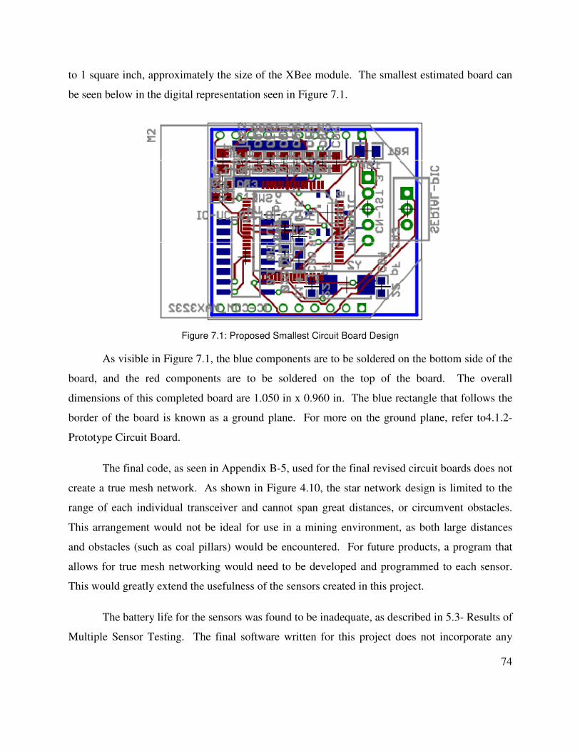
74

to 1 square inch, approximately the size of the XBee module. The smallest estimated board can

be seen below in the digital representation seen in Figure 7.1.

Figure 7.1: Proposed Smallest Circuit Board Design

As visible in Figure 7.1, the blue components are to be soldered on the bottom side of the

board, and the red components are to be soldered on the top of the board. The overall

dimensions of this completed board are 1.050 in x 0.960 in. The blue rectangle that follows the

border of the board is known as a ground plane. For more on the ground plane, refer to4.1.2-

Prototype Circuit Board.

The final code, as seen in Appendix B-5, used for the final revised circuit boards does not

create a true mesh network. As shown in Figure 4.10, the star network design is limited to the

range of each individual transceiver and cannot span great distances, or circumvent obstacles.

This arrangement would not be ideal for use in a mining environment, as both large distances

and obstacles (such as coal pillars) would be encountered. For future products, a program that

allows for true mesh networking would need to be developed and programmed to each sensor.

This would greatly extend the usefulness of the sensors created in this project.

The battery life for the sensors was found to be inadequate, as described in 5.3- Results of

Multiple Sensor Testing. The final software written for this project does not incorporate any

75

sleep modes for the sensors, so they are in essence running 100% of the time. Transmitting data

is by far the greatest consumer of electricity, and although the sensors are not transmitting data at

every given moment, the constant operation of the PIC steadily contributes to battery depletion.

Once the voltage supply dips below 2.1V, the transceiver no longer functions, as the operating

voltage range for the XBee is 2.1V – 3.6V, as described in 4.1.1- Transceiver selection. To

resolve this issue, an external clock would need to be incorporated into the circuit board design.

This external clock would require additional programming, but would allow the circuit board to

essentially cut off all power supply, minus the power needed to run the external clock, and to

reboot itself for sending and receiving data at a given time. Every tiltmeter used in this ideal

product would need to be powered on at relatively the same time, because if data is sent from

sensor A to sensor B, and sensor B is not powered on, the data will not be received, and could

possibly be lost. An external clock would also require a separate power supply, probably a 3V

CR2032 coin cell battery.

Additionally, a “handshake” must be used, or a proximity guide of all operating sensors,

to prevent signals from traveling in opposite directions than the desired endpoint at a PC. Data

could theoretically be transmitted to the very extent of a network and be lost due to sensors

turning on and off if the signal travels the wrong direction. A proximity network would require

additional code, as well as fixed and coordinated locations of each sensor.

Another solution with respect battery life would be to incorporate a small solar panel for

use in surface mines. This solar panel would store energy during the daylight hours and use the

stored energy at night to power the tiltmeter. This solution would also require a method of

relaying wires to the tiltmeter through the protective casing: keeping water and other elements

out of the case would be very important so special care would be needed in designing such a

setup.

A tiltmeter issue that surfaced during discussions with the mining company, see Chapter

6- Field Testing for details, was the concern that a sensitivity of 0.5° might not provide useful

information. It was suggested to find a more sensitive accelerometer, something that could

accurately detect changes of approximately one minute of angle, or 1/60° = 0.01666°. This

76

option was explored lightly, and it was found that more sensitive accelerometers are not readily

available at this time. Some accelerometers do exist with greater sensitivities than those used in

this project, but the associated cost was extreme when compared to the cost of the MXR6999M

accelerometer, as well as the other accelerometers discussed in Chapter 3: Preliminary Data

Collection.

To solve many of these issues, a simple solution is possible. Instead of designing a new

product to replace the tiltmeter of this project, or continuing to experiment and modify the

programming and components of the circuit board, the Accsense sensor pods could be used with

an addition of a more sensitive piece of equipment. As seen in Figure 3.1, the Accsense sensor

pod comes with connection points for additional equipment. Monitoring devices such as

extensometers could be attached to the sensor pod and mounted in such a way that the output

would be sent wirelessly through the sensor pods already existing mesh network. These output

values could still be accessed online, just as described in 3.1- Accsense Wireless Systems.

Though this solution seems rudimentary, it would solve many of the problems associated with

the development of a new device.

77

APPENDIX A: EQUIPMENT TESTING DATA

Accsense Sensitivity Test MEMSIC Frequency Test MEMSIC Sensitivity Test

Multiple Tiltmeter Test Raw Data Multiple Tiltmeter Test Formatted Data

78

Table A.1 shows raw data from the Accsense Sensitivity Tests as described in 3.1- Accsense Wireless Systems.

Table A.1: Accsense Sensitivity Measurements for NE Orientation

5° 10° 15° 20° 25°

Value Time Value Time Value Time Value Time Value Time

17.11 7/6/07 19:31 16.91 7/7/07 10:32 16.72 7/7/07 21:12 16.42 7/8/07 11:08 17.01 7/8/07 18:01

17.01 7/6/07 19:32 16.91 7/7/07 10:33 16.72 7/7/07 21:13 16.52 7/8/07 11:09 16.91 7/8/07 18:02

17.01 7/6/07 19:33 16.91 7/7/07 10:34 16.62 7/7/07 21:14 16.32 7/8/07 11:10 17.01 7/8/07 18:03

17.01 7/6/07 19:34 16.91 7/7/07 10:35 16.72 7/7/07 21:15 16.32 7/8/07 11:11 17.01 7/8/07 18:04

17.01 7/6/07 19:35 16.91 7/7/07 10:36 16.81 7/7/07 21:16 16.42 7/8/07 11:12 17.01 7/8/07 18:05

17.01 7/6/07 19:36 16.72 7/7/07 10:37 16.72 7/7/07 21:17 16.42 7/8/07 11:13 17.01 7/8/07 18:06

17.01 7/6/07 19:37 16.81 7/7/07 10:38 16.72 7/7/07 21:18 16.42 7/8/07 11:14 17.11 7/8/07 18:07

17.01 7/6/07 19:38 16.91 7/7/07 10:39 16.72 7/7/07 21:19 16.32 7/8/07 11:15 17.11 7/8/07 18:08

17.11 7/6/07 19:39 16.91 7/7/07 10:40 16.81 7/7/07 21:20 16.32 7/8/07 11:16 17.01 7/8/07 18:09

17.01 7/6/07 19:40 16.91 7/7/07 10:41 16.72 7/7/07 21:21 16.42 7/8/07 11:17 17.11 7/8/07 18:10

17.01 7/6/07 19:41 16.81 7/7/07 10:42 16.81 7/7/07 21:22 16.42 7/8/07 11:18 17.01 7/8/07 18:11

17.11 7/6/07 19:42 16.81 7/7/07 10:43 16.72 7/7/07 21:23 16.42 7/8/07 11:19 17.11 7/8/07 18:12

17.11 7/6/07 19:43 16.72 7/7/07 10:44 16.72 7/7/07 21:24 16.42 7/8/07 11:20 17.11 7/8/07 18:13

16.91 7/6/07 19:44 16.81 7/7/07 10:45 16.62 7/7/07 21:25 16.32 7/8/07 11:21 17.01 7/8/07 18:14

17.01 7/6/07 19:45 16.81 7/7/07 10:46 16.62 7/7/07 21:26 16.32 7/8/07 11:22 17.01 7/8/07 18:15

17.11 7/6/07 19:46 16.81 7/7/07 10:47 16.62 7/7/07 21:27 16.42 7/8/07 11:23 17.01 7/8/07 18:16

17.11 7/6/07 19:47 16.81 7/7/07 10:48 16.62 7/7/07 21:28 16.52 7/8/07 11:24 17.11 7/8/07 18:17

17.11 7/6/07 19:48 16.72 7/7/07 10:49 16.72 7/7/07 21:29 16.42 7/8/07 11:25 16.91 7/8/07 18:18

17.01 7/6/07 19:49 17.01 7/7/07 10:50 16.72 7/7/07 21:30 16.42 7/8/07 11:26 17.01 7/8/07 18:19

17.01 7/6/07 19:50 16.72 7/7/07 10:51 16.72 7/7/07 21:31 16.42 7/8/07 11:27 17.01 7/8/07 18:20

17.2 7/6/07 19:51 16.91 7/7/07 10:52 16.81 7/7/07 21:32 16.23 7/8/07 11:28 17.11 7/8/07 18:21

17.01 7/6/07 19:52 16.81 7/7/07 10:53 16.81 7/7/07 21:33 16.32 7/8/07 11:29 17.01 7/8/07 18:22

17.01 7/6/07 19:53 16.81 7/7/07 10:54 16.62 7/7/07 21:34 16.42 7/8/07 11:30 17.11 7/8/07 18:23

17.01 7/6/07 19:54 16.91 7/7/07 10:55 16.72 7/7/07 21:35 16.32 7/8/07 11:31 17.01 7/8/07 18:24

17.01 7/6/07 19:55 16.81 7/7/07 10:56 16.72 7/7/07 21:36 16.42 7/8/07 11:32 17.01 7/8/07 18:25

17.01 7/6/07 19:56 16.81 7/7/07 10:57 16.72 7/7/07 21:37 16.42 7/8/07 11:33 17.11 7/8/07 18:26

17.01 7/6/07 19:57 16.72 7/7/07 10:58 16.72 7/7/07 21:38 16.42 7/8/07 11:34 17.01 7/8/07 18:27

17.11 7/6/07 19:58 16.72 7/7/07 10:59 16.81 7/7/07 21:39 16.42 7/8/07 11:35 17.01 7/8/07 18:28

17.01 7/6/07 19:59 16.72 7/7/07 11:00 16.62 7/7/07 21:40 16.42 7/8/07 11:36 17.01 7/8/07 18:29

17.11 7/6/07 20:00 16.91 7/7/07 11:01 16.62 7/7/07 21:41 16.32 7/8/07 11:37 17.01 7/8/07 18:30

17.01 7/6/07 20:01 16.62 7/7/07 21:42 16.32 7/8/07 11:38 17.01 7/8/07 18:31

79

17.01 7/6/07 20:02 µ σ 16.72 7/7/07 21:43 16.32 7/8/07 11:39 17.01 7/8/07 18:32

17.11 7/6/07 20:03 16.83 0.0813118 16.81 7/7/07 21:44 16.42 7/8/07 11:40 17.01 7/8/07 18:33

17.01 7/6/07 20:04 16.62 7/7/07 21:45 16.42 7/8/07 11:41 17.01 7/8/07 18:34

17.11 7/6/07 20:05 16.72 7/7/07 21:46 16.42 7/8/07 11:42 17.01 7/8/07 18:35

17.11 7/6/07 20:06 17.01 7/7/07 21:47 16.42 7/8/07 11:43 17.01 7/8/07 18:36

17.11 7/6/07 20:07 16.81 7/7/07 21:48 16.32 7/8/07 11:44 17.01 7/8/07 18:37

16.91 7/6/07 20:08 16.72 7/7/07 21:49 16.32 7/8/07 11:45 17.2 7/8/07 18:38

17.11 7/6/07 20:09 16.81 7/7/07 21:50 16.52 7/8/07 11:46 17.2 7/8/07 18:39

17.01 7/6/07 20:10 16.72 7/7/07 21:51 16.52 7/8/07 11:47 17.01 7/8/07 18:40

17.01 7/6/07 20:11 16.72 7/7/07 21:52 16.42 7/8/07 11:48 17.11 7/8/07 18:41

16.91 7/6/07 20:12 16.72 7/7/07 21:53 16.52 7/8/07 11:49 17.01 7/8/07 18:42

17.11 7/6/07 20:13 16.72 7/7/07 21:54 16.42 7/8/07 11:50 17.11 7/8/07 18:43

16.91 7/6/07 20:14 16.81 7/7/07 21:55 17.11 7/8/07 18:44

17.11 7/6/07 20:15 16.81 7/7/07 21:56 µ σ 17.01 7/8/07 18:45

17.11 7/6/07 20:16 16.52 7/7/07 21:57 16.4 0.06784207 17.01 7/8/07 18:46

17.11 7/6/07 20:17 16.62 7/7/07 21:58 17.01 7/8/07 18:47

17.11 7/6/07 20:18 16.72 7/7/07 21:59 17.01 7/8/07 18:48

17.11 7/6/07 20:19 16.91 7/7/07 22:00 17.01 7/8/07 18:49

17.01 7/6/07 20:20 16.81 7/7/07 22:01 17.11 7/8/07 18:50

17.11 7/6/07 20:21 16.81 7/7/07 22:02 17.01 7/8/07 18:51

17.11 7/6/07 20:22 16.62 7/7/07 22:03 17.01 7/8/07 18:52

16.91 7/6/07 20:23 16.91 7/7/07 22:04 17.11 7/8/07 18:53

17.11 7/6/07 20:24 16.62 7/7/07 22:05 17.11 7/8/07 18:54

17.11 7/6/07 20:25 16.81 7/7/07 22:06 17.01 7/8/07 18:55

17.01 7/6/07 20:26 16.72 7/7/07 22:07 16.91 7/8/07 18:56

17.01 7/6/07 20:27 16.72 7/7/07 22:08 17.11 7/8/07 18:57

17.11 7/6/07 20:28 16.81 7/7/07 22:09 17.11 7/8/07 18:58

17.01 7/6/07 20:29 16.72 7/7/07 22:10 17.01 7/8/07 18:59

17.01 7/6/07 20:30 16.81 7/7/07 22:11 17.2 7/8/07 19:00

17.11 7/6/07 20:31 16.91 7/7/07 22:12 17.01 7/8/07 19:01

17.01 7/6/07 20:32 16.72 7/7/07 22:13 17.11 7/8/07 19:02

17.2 7/6/07 20:33 16.62 7/7/07 22:14 17.11 7/8/07 19:03

16.81 7/6/07 20:34 16.62 7/7/07 22:15 17.11 7/8/07 19:04

17.01 7/6/07 20:35 16.72 7/7/07 22:16 17.01 7/8/07 19:05

17.01 7/6/07 20:36 16.72 7/7/07 22:17 17.01 7/8/07 19:06

17.01 7/6/07 20:37 16.81 7/7/07 22:18 17.11 7/8/07 19:07

17.2 7/6/07 20:38 16.72 7/7/07 22:19 17.11 7/8/07 19:08

80

17.01 7/6/07 20:39 16.72 7/7/07 22:20 17.01 7/8/07 19:09

17.11 7/6/07 20:40 16.72 7/7/07 22:21 17.11 7/8/07 19:10

16.91 7/6/07 20:41 16.72 7/7/07 22:22 17.11 7/8/07 19:11

16.91 7/6/07 20:42 16.81 7/7/07 22:23 16.91 7/8/07 19:12

17.11 7/6/07 20:43 16.72 7/7/07 22:24 17.01 7/8/07 19:13

17.2 7/6/07 20:44 16.62 7/7/07 22:25 17.01 7/8/07 19:14

16.91 7/6/07 20:45 16.72 7/7/07 22:26 17.01 7/8/07 19:15

17.01 7/6/07 20:46

17.11 7/6/07 20:47 µ σ µ σ

17.01 7/6/07 20:48 16.73 0.08479185 17.04 0.06369635

µ σ

17.04 0.07760098

Figure A.0.1 shows the mean and standard deviation of all data points recorded for each angle at the NE orientation.

Figure A.0.1: NE Mean with ±2 standard deviation error bars

16.2

16.4

16.6

16.8

17

17.2

17.4

5° 10° 15° 20° 25°

Se

nso

r O

utp

ut

(V)

Angle of Inclination (degree)

Accsense: NE Orientation ± 2σ

81


Table A.2: Accsense Sensitivity Measurements for SE Orientation

5° 10° 15° 20° 25°


15.64 7/6/07 23:06 14.08 7/7/07 11:02 12.41 7/7/07 22:29 10.46 7/8/07 11:51 9.091 7/8/07 19:27

15.64 7/6/07 23:07 13.88 7/7/07 11:03 12.32 7/7/07 22:30 10.65 7/8/07 11:52 9.188 7/8/07 19:28

15.84 7/6/07 23:08 13.78 7/7/07 11:04 12.41 7/7/07 22:31 10.56 7/8/07 11:53 9.188 7/8/07 19:29

15.64 7/6/07 23:09 14.08 7/7/07 11:05 12.41 7/7/07 22:32 10.65 7/8/07 11:54 9.188 7/8/07 19:30

15.74 7/6/07 23:10 13.98 7/7/07 11:06 12.41 7/7/07 22:33 10.65 7/8/07 11:55 9.091 7/8/07 19:31

15.54 7/6/07 23:11 13.98 7/7/07 11:07 12.41 7/7/07 22:34 10.65 7/8/07 11:56 9.188 7/8/07 19:32

15.64 7/6/07 23:12 14.08 7/7/07 11:08 12.32 7/7/07 22:35 10.56 7/8/07 11:57 9.188 7/8/07 19:33

15.64 7/6/07 23:13 13.88 7/7/07 11:09 12.32 7/7/07 22:36 10.65 7/8/07 11:58 9.188 7/8/07 19:34

15.74 7/6/07 23:14 14.08 7/7/07 11:10 12.41 7/7/07 22:37 10.56 7/8/07 11:59 9.188 7/8/07 19:35

15.54 7/6/07 23:15 14.08 7/7/07 11:11 12.41 7/7/07 22:38 10.56 7/8/07 12:00 9.188 7/8/07 19:36

15.74 7/6/07 23:16 13.98 7/7/07 11:12 12.41 7/7/07 22:39 10.56 7/8/07 12:01 9.286 7/8/07 19:37

15.74 7/6/07 23:17 14.08 7/7/07 11:13 12.41 7/7/07 22:40 10.65 7/8/07 12:02 9.286 7/8/07 19:38

15.74 7/6/07 23:18 14.08 7/7/07 11:14 12.51 7/7/07 22:41 10.56 7/8/07 12:03 9.091 7/8/07 19:39

15.44 7/6/07 23:19 13.98 7/7/07 11:15 12.22 7/7/07 22:42 10.46 7/8/07 12:04 9.091 7/8/07 19:40

15.64 7/6/07 23:20 13.98 7/7/07 11:16 12.32 7/7/07 22:43 10.56 7/8/07 12:05 8.993 7/8/07 19:41

15.54 7/6/07 23:21 13.98 7/7/07 11:17 12.41 7/7/07 22:44 10.56 7/8/07 12:06 9.188 7/8/07 19:42

15.54 7/6/07 23:22 13.98 7/7/07 11:18 12.41 7/7/07 22:45 10.46 7/8/07 12:07 9.188 7/8/07 19:43

15.64 7/6/07 23:23 13.88 7/7/07 11:19 12.51 7/7/07 22:46 10.56 7/8/07 12:08 9.188 7/8/07 19:44

15.64 7/6/07 23:24 13.88 7/7/07 11:20 12.41 7/7/07 22:47 10.56 7/8/07 12:09 9.286 7/8/07 19:45

15.64 7/6/07 23:25 13.98 7/7/07 11:21 12.32 7/7/07 22:48 10.65 7/8/07 12:10 9.091 7/8/07 19:46

15.64 7/6/07 23:26 13.98 7/7/07 11:22 12.41 7/7/07 22:49 10.65 7/8/07 12:11 9.091 7/8/07 19:47

15.84 7/6/07 23:27 13.88 7/7/07 11:23 12.41 7/7/07 22:50 10.56 7/8/07 12:12 9.188 7/8/07 19:48

15.64 7/6/07 23:28 13.88 7/7/07 11:24 12.32 7/7/07 22:51 10.46 7/8/07 12:13 9.091 7/8/07 19:49

15.54 7/6/07 23:29 13.98 7/7/07 11:25 12.51 7/7/07 22:52 10.56 7/8/07 12:14 9.286 7/8/07 19:50

15.74 7/6/07 23:30 14.08 7/7/07 11:26 12.41 7/7/07 22:53 10.56 7/8/07 12:15 9.091 7/8/07 19:51

15.54 7/6/07 23:31 14.17 7/7/07 11:27 12.51 7/7/07 22:54 10.56 7/8/07 12:16 9.286 7/8/07 19:52

15.74 7/6/07 23:32 13.98 7/7/07 11:28 12.32 7/7/07 22:55 10.56 7/8/07 12:17 9.091 7/8/07 19:53

15.64 7/6/07 23:33 13.98 7/7/07 11:29 12.51 7/7/07 22:56 10.56 7/8/07 12:18 9.188 7/8/07 19:54

15.74 7/6/07 23:34 14.08 7/7/07 11:30 12.41 7/7/07 22:57 10.75 7/8/07 12:19 8.993 7/8/07 19:55

82

15.64 7/6/07 23:35 13.98 7/7/07 11:31 12.41 7/7/07 22:58 10.56 7/8/07 12:20 9.091 7/8/07 19:56

15.64 7/6/07 23:36 14.08 7/7/07 11:32 12.41 7/7/07 22:59 10.56 7/8/07 12:21 9.188 7/8/07 19:57

15.54 7/6/07 23:37 14.08 7/7/07 11:33 12.41 7/7/07 23:00 10.56 7/8/07 12:22 9.188 7/8/07 19:58

15.84 7/6/07 23:38 13.98 7/7/07 11:34 12.51 7/7/07 23:01 10.65 7/8/07 12:23 9.091 7/8/07 19:59

15.74 7/6/07 23:39 14.08 7/7/07 11:35 12.32 7/7/07 23:02 10.46 7/8/07 12:24 9.188 7/8/07 20:00

15.74 7/6/07 23:40 13.88 7/7/07 11:36 12.41 7/7/07 23:03 10.46 7/8/07 12:25 9.091 7/8/07 20:01

15.74 7/6/07 23:41 13.88 7/7/07 11:37 12.41 7/7/07 23:04 10.56 7/8/07 12:26 9.091 7/8/07 20:02

15.64 7/6/07 23:42 13.88 7/7/07 11:38 12.41 7/7/07 23:05 10.65 7/8/07 12:27 9.091 7/8/07 20:03

15.74 7/6/07 23:43 13.98 7/7/07 11:39 12.41 7/7/07 23:06 10.65 7/8/07 12:28 9.188 7/8/07 20:04

15.64 7/6/07 23:44 13.98 7/7/07 11:40 12.41 7/7/07 23:07 10.46 7/8/07 12:29 9.286 7/8/07 20:05

15.74 7/6/07 23:45 13.98 7/7/07 11:41 12.51 7/7/07 23:08 10.56 7/8/07 12:30 9.188 7/8/07 20:06

15.54 7/6/07 23:46 14.08 7/7/07 11:42 12.41 7/7/07 23:09 10.56 7/8/07 12:31 9.188 7/8/07 20:07

15.74 7/6/07 23:47 14.08 7/7/07 11:43 12.41 7/7/07 23:10 10.56 7/8/07 12:32 9.188 7/8/07 20:08

13.88 7/7/07 11:44 12.41 7/7/07 23:11 10.46 7/8/07 12:33 9.091 7/8/07 20:09

µ σ 13.98 7/7/07 11:45 12.51 7/7/07 23:12 10.65 7/8/07 12:34 8.993 7/8/07 20:10

15.66 0.09320715 14.08 7/7/07 11:46 12.41 7/7/07 23:13 10.75 7/8/07 12:35 9.188 7/8/07 20:11

13.98 7/7/07 11:47 12.51 7/7/07 23:14 10.46 7/8/07 12:36 9.188 7/8/07 20:12

13.98 7/7/07 11:48 12.32 7/7/07 23:15 10.65 7/8/07 12:37 9.188 7/8/07 20:13

13.88 7/7/07 11:49 12.41 7/7/07 23:16 10.65 7/8/07 12:38 9.286 7/8/07 20:14

13.78 7/7/07 11:50 12.41 7/7/07 23:17 10.65 7/8/07 12:39 9.188 7/8/07 20:15

13.98 7/7/07 11:51 12.32 7/7/07 23:18 10.65 7/8/07 12:40 9.091 7/8/07 20:16

14.08 7/7/07 11:52 12.51 7/7/07 23:19 10.56 7/8/07 12:41 9.091 7/8/07 20:17

13.98 7/7/07 11:53 12.61 7/7/07 23:20 10.56 7/8/07 12:42 9.188 7/8/07 20:18

13.98 7/7/07 11:54 12.41 7/7/07 23:21 10.65 7/8/07 12:43 9.091 7/8/07 20:19

13.98 7/7/07 11:55 12.41 7/7/07 23:22 10.56 7/8/07 12:44 8.993 7/8/07 20:20

13.88 7/7/07 11:56 12.32 7/7/07 23:23 10.65 7/8/07 12:45 9.188 7/8/07 20:21

13.88 7/7/07 11:57 12.41 7/7/07 23:24 10.65 7/8/07 12:46 9.286 7/8/07 20:22

13.88 7/7/07 11:58 12.41 7/7/07 23:25 10.65 7/8/07 12:47 9.188 7/8/07 20:23

13.98 7/7/07 11:59 12.61 7/7/07 23:26 10.56 7/8/07 12:48 9.091 7/8/07 20:24

13.98 7/7/07 12:00 12.41 7/7/07 23:27 10.56 7/8/07 12:49 9.188 7/8/07 20:25

14.08 7/7/07 12:01 12.41 7/7/07 23:28 10.46 7/8/07 12:50 9.188 7/8/07 20:26

13.98 7/7/07 12:02 12.32 7/7/07 23:29 10.46 7/8/07 12:51 9.286 7/8/07 20:27

13.98 7/7/07 12:03 12.32 7/7/07 23:30 10.56 7/8/07 12:52 9.384 7/8/07 20:28

14.08 7/7/07 12:04 12.41 7/7/07 23:31 10.65 7/8/07 12:53 9.188 7/8/07 20:29

14.08 7/7/07 12:05 12.41 7/7/07 23:32 10.56 7/8/07 12:54 8.993 7/8/07 20:30

13.98 7/7/07 12:06 12.51 7/7/07 23:33 10.56 7/8/07 12:55 9.091 7/8/07 20:31

13.98 7/7/07 12:07 12.51 7/7/07 23:34 10.65 7/8/07 12:56 9.091 7/8/07 20:32

83

14.08 7/7/07 12:08 12.32 7/7/07 23:35 10.65 7/8/07 12:57 9.188 7/8/07 20:33

14.08 7/7/07 12:09 12.41 7/7/07 23:36 10.46 7/8/07 12:58 9.091 7/8/07 20:34

13.98 7/7/07 12:10 12.51 7/7/07 23:37 10.65 7/8/07 12:59 9.188 7/8/07 20:35

13.88 7/7/07 12:11 12.32 7/7/07 23:38 10.56 7/8/07 13:00 9.091 7/8/07 20:36

13.88 7/7/07 12:12 12.32 7/7/07 23:39 10.65 7/8/07 13:01 9.091 7/8/07 20:37

13.98 7/7/07 12:13 12.41 7/7/07 23:40 10.65 7/8/07 13:02 9.188 7/8/07 20:38

13.88 7/7/07 12:14 12.32 7/7/07 23:41 10.56 7/8/07 13:03 9.188 7/8/07 20:39

13.88 7/7/07 12:15 12.32 7/7/07 23:42 10.56 7/8/07 13:04 9.188 7/8/07 20:40

14.08 7/7/07 12:16 12.41 7/7/07 23:43 10.65 7/8/07 13:05 9.188 7/8/07 20:41

14.08 7/7/07 12:17 12.32 7/7/07 23:44 10.56 7/8/07 13:06 9.091 7/8/07 20:42

13.88 7/7/07 12:18 12.51 7/7/07 23:45 10.46 7/8/07 13:07 9.188 7/8/07 20:43

14.08 7/7/07 12:19 12.41 7/7/07 23:46 10.56 7/8/07 13:08 9.091 7/8/07 20:44

13.98 7/7/07 12:20 12.22 7/7/07 23:47 10.56 7/8/07 13:09 9.091 7/8/07 20:45

13.98 7/7/07 12:21 12.41 7/7/07 23:48 10.46 7/8/07 13:10

13.98 7/7/07 12:22 12.51 7/7/07 23:49 10.75 7/8/07 13:11 µ σ

13.98 7/7/07 12:23 12.41 7/7/07 23:50 10.65 7/8/07 13:12 9.156 0.07916958

13.98 7/7/07 12:24 10.56 7/8/07 13:13

13.88 7/7/07 12:25 µ σ 10.46 7/8/07 13:14

13.88 7/7/07 12:26 12.41 0.07500286 10.65 7/8/07 13:15

13.88 7/7/07 12:27 10.56 7/8/07 13:16

13.88 7/7/07 12:28 10.56 7/8/07 13:17

13.88 7/7/07 12:29 10.75 7/8/07 13:18

13.98 7/7/07 12:30 10.46 7/8/07 13:19

13.88 7/7/07 12:31 10.46 7/8/07 13:20

13.98 7/7/07 12:32 10.65 7/8/07 13:21

13.98 7/7/07 12:33 10.65 7/8/07 13:22

13.88 7/7/07 12:34 10.65 7/8/07 13:23

13.98 7/7/07 12:35 10.65 7/8/07 13:24

14.08 7/7/07 12:36 10.56 7/8/07 13:25

14.08 7/7/07 12:37 10.65 7/8/07 13:26

13.98 7/7/07 12:38 10.56 7/8/07 13:27

13.98 7/7/07 12:39 10.46 7/8/07 13:28

14.08 7/7/07 12:40 10.56 7/8/07 13:29

14.08 7/7/07 12:41 10.56 7/8/07 13:30

13.98 7/7/07 12:42 10.65 7/8/07 13:31

13.98 7/7/07 12:43 10.65 7/8/07 13:32

84

13.88 7/7/07 12:44 10.65 7/8/07 13:33

13.88 7/7/07 12:45 10.46 7/8/07 13:34

13.88 7/7/07 12:46

13.98 7/7/07 12:47 µ σ

13.98 7/7/07 12:48 10.58 0.07555514

14.17 7/7/07 12:49

14.08 7/7/07 12:50

14.08 7/7/07 12:51

13.98 7/7/07 12:52

µ σ

13.98 0.08213859

Figure A.0.2 shows the mean and standard deviation of all data points recorded for each angle at the SE orientation.

Figure A.0.2: SE Mean with ±2 standard deviation error bars

8

9

10

11

12

13

14

15

16

17

5° 10° 15° 20° 25°

Se

nso

r O

utp

ut

(V)


Accsense: SE Orientation ±2σ

85


Table A.3: Accsense Sensitivity Measurements for SW Orientation

5° 10° 15° 20° 25°


17.69 7/6/07 20:51 17.79 7/7/07 18:48 17.3 7/7/07 23:53 17.01 7/8/07 13:46 16.32 7/8/07 20:52

17.69 7/6/07 20:52 17.6 7/7/07 18:49 17.2 7/7/07 23:54 16.91 7/8/07 13:47 16.52 7/8/07 20:53

17.6 7/6/07 20:53 17.6 7/7/07 18:50 17.3 7/7/07 23:55 17.01 7/8/07 13:48 16.32 7/8/07 20:54

17.69 7/6/07 20:54 17.5 7/7/07 18:51 17.4 7/7/07 23:56 17.01 7/8/07 13:49 16.42 7/8/07 20:55

17.69 7/6/07 20:55 17.5 7/7/07 18:52 17.4 7/7/07 23:57 16.81 7/8/07 13:50 16.42 7/8/07 20:56

17.69 7/6/07 20:56 17.6 7/7/07 18:53 17.5 7/7/07 23:58 16.81 7/8/07 13:51 16.42 7/8/07 20:57

17.79 7/6/07 20:57 17.6 7/7/07 18:54 17.2 7/7/07 23:59 16.91 7/8/07 13:52 16.42 7/8/07 20:58

17.69 7/6/07 20:58 17.6 7/7/07 18:55 17.3 7/8/07 0:00 16.91 7/8/07 13:53 16.42 7/8/07 20:59

17.69 7/6/07 20:59 17.6 7/7/07 18:56 17.4 7/8/07 0:01 16.91 7/8/07 13:54 16.32 7/8/07 21:00

17.69 7/6/07 21:00 17.5 7/7/07 18:57 17.3 7/8/07 0:02 16.91 7/8/07 13:55 16.52 7/8/07 21:01

17.79 7/6/07 21:01 17.69 7/7/07 18:58 17.3 7/8/07 0:03 17.01 7/8/07 13:56 16.23 7/8/07 21:02

17.69 7/6/07 21:02 17.6 7/7/07 18:59 17.3 7/8/07 0:04 16.91 7/8/07 13:57 16.42 7/8/07 21:03

17.6 7/6/07 21:03 17.6 7/7/07 19:00 17.4 7/8/07 0:05 16.91 7/8/07 13:58 16.52 7/8/07 21:04

17.79 7/6/07 21:04 17.79 7/7/07 19:01 17.4 7/8/07 0:06 16.81 7/8/07 13:59 16.42 7/8/07 21:05

17.69 7/6/07 21:05 17.6 7/7/07 19:02 17.4 7/8/07 0:07 17.01 7/8/07 14:00 16.42 7/8/07 21:06

17.79 7/6/07 21:06 17.6 7/7/07 19:03 17.4 7/8/07 0:08 17.01 7/8/07 14:01 16.42 7/8/07 21:07

17.79 7/6/07 21:07 17.79 7/7/07 19:04 17.3 7/8/07 0:09 17.01 7/8/07 14:02 16.32 7/8/07 21:08

17.69 7/6/07 21:08 17.6 7/7/07 19:05 17.3 7/8/07 0:10 17.01 7/8/07 14:03 16.52 7/8/07 21:09

17.79 7/6/07 21:09 17.6 7/7/07 19:06 17.4 7/8/07 0:11 16.91 7/8/07 14:04 16.52 7/8/07 21:10

17.69 7/6/07 21:10 17.5 7/7/07 19:07 17.3 7/8/07 0:12 17.11 7/8/07 14:05 16.42 7/8/07 21:11

17.79 7/6/07 21:11 17.6 7/7/07 19:08 17.3 7/8/07 0:13 16.91 7/8/07 14:06 16.52 7/8/07 21:12

17.79 7/6/07 21:12 17.69 7/7/07 19:09 17.2 7/8/07 0:14 17.01 7/8/07 14:07 16.42 7/8/07 21:13

17.69 7/6/07 21:13 17.79 7/7/07 19:10 17.2 7/8/07 0:15 16.81 7/8/07 14:08 16.42 7/8/07 21:14

17.79 7/6/07 21:14 17.6 7/7/07 19:11 17.4 7/8/07 0:16 16.81 7/8/07 14:09 16.42 7/8/07 21:15

17.79 7/6/07 21:15 17.6 7/7/07 19:12 17.4 7/8/07 0:17 17.01 7/8/07 14:10 16.42 7/8/07 21:16

17.79 7/6/07 21:16 17.6 7/7/07 19:13 17.4 7/8/07 0:18 17.01 7/8/07 14:11 16.42 7/8/07 21:17

17.69 7/6/07 21:17 17.5 7/7/07 19:14 17.4 7/8/07 0:19 16.91 7/8/07 14:12 16.32 7/8/07 21:18

17.69 7/6/07 21:18 17.6 7/7/07 19:15 17.2 7/8/07 0:20 16.91 7/8/07 14:13 16.42 7/8/07 21:19

17.69 7/6/07 21:19 17.6 7/7/07 19:16 17.3 7/8/07 0:21 17.01 7/8/07 14:14 16.42 7/8/07 21:20

17.69 7/6/07 21:20 17.69 7/7/07 19:17 17.3 7/8/07 0:22 17.01 7/8/07 14:15 16.42 7/8/07 21:21

17.79 7/6/07 21:21 17.5 7/7/07 19:18 17.4 7/8/07 0:23 17.01 7/8/07 14:16 16.52 7/8/07 21:22

86

17.79 7/6/07 21:22 17.6 7/7/07 19:19 17.2 7/8/07 0:24 16.91 7/8/07 14:17 16.52 7/8/07 21:23

17.79 7/6/07 21:23 17.6 7/7/07 19:20 17.3 7/8/07 0:25 16.91 7/8/07 14:18 16.52 7/8/07 21:24

17.69 7/6/07 21:24 17.6 7/7/07 19:21 17.3 7/8/07 0:26 17.01 7/8/07 14:19 16.42 7/8/07 21:25

17.79 7/6/07 21:25 17.6 7/7/07 19:22 17.2 7/8/07 0:27 17.01 7/8/07 14:20 16.62 7/8/07 21:26

17.69 7/6/07 21:26 17.5 7/7/07 19:23 17.3 7/8/07 0:28 17.01 7/8/07 14:21 16.42 7/8/07 21:27

17.69 7/6/07 21:27 17.5 7/7/07 19:24 17.2 7/8/07 0:29 16.91 7/8/07 14:22 16.32 7/8/07 21:28

17.69 7/6/07 21:28 17.5 7/7/07 19:25 17.4 7/8/07 0:30 17.01 7/8/07 14:23 16.52 7/8/07 21:29

17.69 7/6/07 21:29 17.6 7/7/07 19:26 17.2 7/8/07 0:31 17.01 7/8/07 14:24 16.42 7/8/07 21:30

17.69 7/6/07 21:30 17.69 7/7/07 19:27 17.3 7/8/07 0:32 17.01 7/8/07 14:25 16.42 7/8/07 21:31

17.79 7/6/07 21:31 17.5 7/7/07 19:28 17.11 7/8/07 0:33 17.01 7/8/07 14:26 16.52 7/8/07 21:32

17.6 7/6/07 21:32 17.69 7/7/07 19:29 17.3 7/8/07 0:34 17.01 7/8/07 14:27 16.42 7/8/07 21:33

17.79 7/6/07 21:33 17.69 7/7/07 19:30 17.3 7/8/07 0:35 17.01 7/8/07 14:28 16.52 7/8/07 21:34

17.69 7/6/07 21:34 17.5 7/7/07 19:31 17.4 7/8/07 0:36 17.11 7/8/07 14:29 16.62 7/8/07 21:35

17.79 7/6/07 21:35 17.6 7/7/07 19:32 17.3 7/8/07 0:37 16.81 7/8/07 14:30 16.42 7/8/07 21:36

17.69 7/6/07 21:36 17.69 7/7/07 19:33 17.4 7/8/07 0:38 17.01 7/8/07 14:31 16.42 7/8/07 21:37

17.79 7/6/07 21:37 17.6 7/7/07 19:34 17.2 7/8/07 0:39 17.01 7/8/07 14:32 16.52 7/8/07 21:38

17.89 7/6/07 21:38 17.69 7/7/07 19:35 17.3 7/8/07 0:40 16.91 7/8/07 14:33 16.52 7/8/07 21:39

17.69 7/6/07 21:39 17.69 7/7/07 19:36 17.3 7/8/07 0:41 17.01 7/8/07 14:34 16.42 7/8/07 21:40

17.79 7/6/07 21:40 17.5 7/7/07 19:37 17.4 7/8/07 0:42 17.01 7/8/07 14:35 16.42 7/8/07 21:41

17.69 7/6/07 21:41 17.69 7/7/07 19:38 17.4 7/8/07 0:43 16.91 7/8/07 14:36 16.52 7/8/07 21:42

17.79 7/6/07 21:42 17.5 7/7/07 19:39 17.4 7/8/07 0:44 16.91 7/8/07 14:37 16.42 7/8/07 21:43

17.69 7/6/07 21:43 17.5 7/7/07 19:40 17.3 7/8/07 0:45 17.01 7/8/07 14:38 16.42 7/8/07 21:44

17.69 7/6/07 21:44 17.6 7/7/07 19:41 17.4 7/8/07 0:46 16.91 7/8/07 14:39 16.52 7/8/07 21:45

17.69 7/6/07 21:45 17.6 7/7/07 19:42 17.4 7/8/07 0:47 16.91 7/8/07 14:40 16.52 7/8/07 21:46

17.79 7/6/07 21:46 17.6 7/7/07 19:43 17.2 7/8/07 0:48 17.11 7/8/07 14:41 16.42 7/8/07 21:47

17.6 7/6/07 21:47 17.4 7/8/07 0:49 17.01 7/8/07 14:42 16.52 7/8/07 21:48

17.69 7/6/07 21:48 µ σ 17.2 7/8/07 0:50 16.81 7/8/07 14:43 16.42 7/8/07 21:49

17.79 7/6/07 21:49 17.6 0.08137376 17.4 7/8/07 0:51 16.91 7/8/07 14:44 16.52 7/8/07 21:50

17.69 7/6/07 21:50 17.4 7/8/07 0:52 17.01 7/8/07 14:45 16.52 7/8/07 21:51

17.79 7/6/07 21:51 17.11 7/8/07 0:53 16.81 7/8/07 14:46 16.52 7/8/07 21:52

17.69 7/6/07 21:52 17.4 7/8/07 0:54 16.91 7/8/07 14:47 16.62 7/8/07 21:53

17.69 7/6/07 21:53 17.4 7/8/07 0:55 16.91 7/8/07 14:48 16.42 7/8/07 21:54

17.79 7/6/07 21:54 17.3 7/8/07 0:56 17.01 7/8/07 14:49 16.52 7/8/07 21:55

17.79 7/6/07 21:55 17.3 7/8/07 0:57 16.91 7/8/07 14:50 16.62 7/8/07 21:56

17.69 7/6/07 21:56 17.3 7/8/07 0:58 16.91 7/8/07 14:51 16.52 7/8/07 21:57

17.69 7/6/07 21:57 17.3 7/8/07 0:59 16.91 7/8/07 14:52 16.42 7/8/07 21:58

17.6 7/6/07 21:58 17.4 7/8/07 1:00 17.01 7/8/07 14:53 16.52 7/8/07 21:59

87

17.79 7/6/07 21:59 17.3 7/8/07 1:01 16.81 7/8/07 14:54 16.42 7/8/07 22:00

17.6 7/6/07 22:00 17.3 7/8/07 1:02 17.01 7/8/07 14:55 16.32 7/8/07 22:01

17.69 7/6/07 22:01 17.3 7/8/07 1:03 17.01 7/8/07 14:56 16.32 7/8/07 22:02

17.79 7/6/07 22:02 17.2 7/8/07 1:04 17.01 7/8/07 14:57 16.52 7/8/07 22:03

17.69 7/6/07 22:03 17.3 7/8/07 1:05 16.72 7/8/07 14:58 16.62 7/8/07 22:04

17.79 7/6/07 22:04 17.2 7/8/07 1:06 16.91 7/8/07 14:59 16.52 7/8/07 22:05

17.6 7/6/07 22:05 17.2 7/8/07 1:07 16.91 7/8/07 15:00 16.52 7/8/07 22:06

17.79 7/6/07 22:06 17.11 7/8/07 1:08 17.01 7/8/07 15:01 16.62 7/8/07 22:07

17.6 7/6/07 22:07 17.3 7/8/07 1:09 16.91 7/8/07 15:02 16.42 7/8/07 22:08

17.79 7/6/07 22:08 17.3 7/8/07 1:10 16.81 7/8/07 15:03 16.52 7/8/07 22:09

17.69 7/6/07 22:09 17.3 7/8/07 1:11 16.91 7/8/07 15:04 16.52 7/8/07 22:10

17.69 7/6/07 22:10 17.4 7/8/07 1:12 17.01 7/8/07 15:05 16.42 7/8/07 22:11

17.69 7/6/07 22:11 17.4 7/8/07 1:13 16.91 7/8/07 15:06 16.52 7/8/07 22:12

17.69 7/6/07 22:12 17.3 7/8/07 1:14 17.01 7/8/07 15:07 16.42 7/8/07 22:13

17.6 7/6/07 22:13 17.3 7/8/07 1:15 16.91 7/8/07 15:08 16.52 7/8/07 22:14

17.79 7/6/07 22:14 17.2 7/8/07 1:16 16.91 7/8/07 15:09 16.52 7/8/07 22:15

17.69 7/6/07 22:15 17.11 7/8/07 1:17 16.91 7/8/07 15:10 16.52 7/8/07 22:16

17.79 7/6/07 22:16 17.4 7/8/07 1:18 16.91 7/8/07 15:11 16.42 7/8/07 22:17

17.6 7/6/07 22:17 17.3 7/8/07 1:19 16.81 7/8/07 15:12 16.62 7/8/07 22:18

17.6 7/6/07 22:18 17.2 7/8/07 1:20 16.91 7/8/07 15:13 16.52 7/8/07 22:19

17.79 7/6/07 22:19 17.4 7/8/07 1:21 16.81 7/8/07 15:14 16.42 7/8/07 22:20

17.69 7/6/07 22:20 17.4 7/8/07 1:22 16.81 7/8/07 15:15 16.52 7/8/07 22:21

17.69 7/6/07 22:21 17.3 7/8/07 1:23 16.91 7/8/07 15:16 16.52 7/8/07 22:22

17.6 7/6/07 22:22 17.2 7/8/07 1:24 17.01 7/8/07 15:17 16.52 7/8/07 22:23

17.79 7/6/07 22:23 17.2 7/8/07 1:25 17.01 7/8/07 15:18 16.42 7/8/07 22:24

17.69 7/6/07 22:24 17.2 7/8/07 1:26 16.91 7/8/07 15:19 16.52 7/8/07 22:25

17.79 7/6/07 22:25 17.5 7/8/07 1:27 16.91 7/8/07 15:20 16.42 7/8/07 22:26

17.69 7/6/07 22:26 17.11 7/8/07 1:28 16.52 7/8/07 22:27

17.69 7/6/07 22:27 17.2 7/8/07 1:29 µ σ 16.42 7/8/07 22:28

17.79 7/6/07 22:28 17.11 7/8/07 1:30 16.94 0.07884056 16.42 7/8/07 22:29

17.69 7/6/07 22:29 17.2 7/8/07 1:31 16.52 7/8/07 22:30

17.89 7/6/07 22:30 17.3 7/8/07 1:32 16.52 7/8/07 22:31

17.79 7/6/07 22:31 17.4 7/8/07 1:33 16.52 7/8/07 22:32

17.79 7/6/07 22:32 17.3 7/8/07 1:34 16.52 7/8/07 22:33

17.69 7/6/07 22:33 17.3 7/8/07 1:35 16.42 7/8/07 22:34

17.69 7/6/07 22:34 17.3 7/8/07 1:36 16.32 7/8/07 22:35

17.79 7/6/07 22:35 17.3 7/8/07 1:37 16.52 7/8/07 22:36

88

17.79 7/6/07 22:36 17.2 7/8/07 1:38 16.32 7/8/07 22:37

17.79 7/6/07 22:37 17.4 7/8/07 1:39 16.42 7/8/07 22:38

17.69 7/6/07 22:38 17.4 7/8/07 1:40 16.42 7/8/07 22:39

17.79 7/6/07 22:39 17.3 7/8/07 1:41 16.62 7/8/07 22:40

17.79 7/6/07 22:40 17.4 7/8/07 1:42 16.52 7/8/07 22:41

17.79 7/6/07 22:41 17.5 7/8/07 1:43 16.32 7/8/07 22:42

17.79 7/6/07 22:42 17.4 7/8/07 1:44 16.42 7/8/07 22:43

17.69 7/6/07 22:43 17.3 7/8/07 1:45 16.42 7/8/07 22:44

17.69 7/6/07 22:44 17.3 7/8/07 1:46 16.52 7/8/07 22:45

17.79 7/6/07 22:45 17.3 7/8/07 1:47 16.42 7/8/07 22:46

17.89 7/6/07 22:46 17.4 7/8/07 1:48 16.42 7/8/07 22:47

17.79 7/6/07 22:47 17.2 7/8/07 1:49 16.62 7/8/07 22:48

17.69 7/6/07 22:48 17.3 7/8/07 1:50 16.32 7/8/07 22:49

17.69 7/6/07 22:49 17.3 7/8/07 1:51 16.42 7/8/07 22:50

17.79 7/6/07 22:50 17.11 7/8/07 1:52 16.62 7/8/07 22:51

17.69 7/6/07 22:51 17.4 7/8/07 1:53 16.52 7/8/07 22:52

17.79 7/6/07 22:52 17.2 7/8/07 1:54 16.52 7/8/07 22:53

17.6 7/6/07 22:53 17.3 7/8/07 1:55 16.42 7/8/07 22:54

17.79 7/6/07 22:54 17.3 7/8/07 1:56 16.42 7/8/07 22:55

17.69 7/6/07 22:55 17.4 7/8/07 1:57 16.42 7/8/07 22:56

17.79 7/6/07 22:56 17.3 7/8/07 1:58 16.42 7/8/07 22:57

17.6 7/6/07 22:57 17.4 7/8/07 1:59 16.62 7/8/07 22:58

17.69 7/6/07 22:58 17.11 7/8/07 2:00 16.52 7/8/07 22:59

17.69 7/6/07 22:59 17.3 7/8/07 2:01 16.52 7/8/07 23:00

17.79 7/6/07 23:00 17.4 7/8/07 2:02 16.62 7/8/07 23:01

17.79 7/6/07 23:01 17.2 7/8/07 2:03 16.52 7/8/07 23:02

17.69 7/6/07 23:02 17.2 7/8/07 2:04

17.69 7/6/07 23:03 17.3 7/8/07 2:05 µ σ

17.69 7/6/07 23:04 17.4 7/8/07 2:06 16.47 0.08138806

17.2 7/8/07 2:07

µ σ 17.4 7/8/07 2:08

17.73 0.06748608 17.4 7/8/07 2:09

17.3 7/8/07 2:10

17.5 7/8/07 2:11

17.4 7/8/07 2:12

17.3 7/8/07 2:13

89

µ σ

17.31 0.09182778

0.18365555

Figure A.0.3 shows the mean and standard deviation of all data points recorded for each angle at the SW orientation.

Figure A.0.3: SW Mean with ±2 standard deviation error bars

15.5

16

16.5

17

17.5

18

5° 10° 15° 20° 25°

Se

nso

r O

utp

ut

(V)


Accsense: SW Orientation ±2σ

90


Table A.4: Accsense Sensitivity Measurements for NW Orientation

5° 10°: 15° 20° 25°


19.26 7/6/07 23:51 20.43 7/7/07 19:46 20.53 7/8/07 4:36 22.58 7/8/07 15:26 23.56 7/8/07 23:08

19.06 7/6/07 23:52 20.33 7/7/07 19:47 20.43 7/8/07 4:37 22.58 7/8/07 15:27 23.66 7/8/07 23:09

18.96 7/6/07 23:53 20.43 7/7/07 19:48 20.63 7/8/07 4:38 22.58 7/8/07 15:28 23.46 7/8/07 23:10

19.06 7/6/07 23:54 20.43 7/7/07 19:49 20.53 7/8/07 4:39 22.58 7/8/07 15:29 23.46 7/8/07 23:11

19.06 7/6/07 23:55 20.43 7/7/07 19:50 20.53 7/8/07 4:40 22.58 7/8/07 15:30 23.46 7/8/07 23:12

19.06 7/6/07 23:56 20.33 7/7/07 19:51 20.53 7/8/07 4:41 22.58 7/8/07 15:31 23.46 7/8/07 23:13

19.16 7/6/07 23:57 20.33 7/7/07 19:52 20.53 7/8/07 4:42 22.58 7/8/07 15:32 23.56 7/8/07 23:14

19.16 7/6/07 23:58 20.33 7/7/07 19:53 20.43 7/8/07 4:43 22.48 7/8/07 15:33 23.56 7/8/07 23:15

19.16 7/6/07 23:59 20.23 7/7/07 19:54 20.53 7/8/07 4:44 22.68 7/8/07 15:34 23.56 7/8/07 23:16

19.06 7/7/07 0:00 20.33 7/7/07 19:55 20.43 7/8/07 4:45 22.48 7/8/07 15:35 23.36 7/8/07 23:17

19.16 7/7/07 0:01 20.23 7/7/07 19:56 20.53 7/8/07 4:46 22.68 7/8/07 15:36 23.46 7/8/07 23:18

19.06 7/7/07 0:02 20.43 7/7/07 19:57 20.53 7/8/07 4:47 22.58 7/8/07 15:37 23.56 7/8/07 23:19

19.06 7/7/07 0:03 20.33 7/7/07 19:58 20.53 7/8/07 4:48 22.58 7/8/07 15:38 23.46 7/8/07 23:20

19.16 7/7/07 0:04 20.33 7/7/07 19:59 20.53 7/8/07 4:49 22.68 7/8/07 15:39 23.56 7/8/07 23:21

19.16 7/7/07 0:05 20.43 7/7/07 20:00 20.63 7/8/07 4:50 22.68 7/8/07 15:40 23.56 7/8/07 23:22

19.06 7/7/07 0:06 20.33 7/7/07 20:01 20.43 7/8/07 4:51 22.58 7/8/07 15:41 23.56 7/8/07 23:23

19.16 7/7/07 0:07 20.33 7/7/07 20:02 20.53 7/8/07 4:52 22.58 7/8/07 15:42 23.46 7/8/07 23:24

19.06 7/7/07 0:08 20.14 7/7/07 20:03 20.53 7/8/07 4:53 22.58 7/8/07 15:43 23.46 7/8/07 23:25

19.16 7/7/07 0:09 20.43 7/7/07 20:04 20.53 7/8/07 4:54 22.68 7/8/07 15:44 23.46 7/8/07 23:26

19.06 7/7/07 0:10 20.43 7/7/07 20:05 20.43 7/8/07 4:55 22.68 7/8/07 15:45 23.56 7/8/07 23:27

18.96 7/7/07 0:11 20.43 7/7/07 20:06 20.53 7/8/07 4:56 22.58 7/8/07 15:46 23.46 7/8/07 23:28

19.06 7/7/07 0:12 20.33 7/7/07 20:07 20.53 7/8/07 4:57 22.68 7/8/07 15:47 23.56 7/8/07 23:29

19.06 7/7/07 0:13 20.33 7/7/07 20:08 20.63 7/8/07 4:58 22.68 7/8/07 15:48 23.56 7/8/07 23:30

19.16 7/7/07 0:14 20.53 7/7/07 20:09 20.53 7/8/07 4:59 22.58 7/8/07 15:49 23.75 7/8/07 23:31

19.16 7/7/07 0:15 20.43 7/7/07 20:10 20.63 7/8/07 5:00 22.58 7/8/07 15:50 23.36 7/8/07 23:32

19.16 7/7/07 0:16 20.33 7/7/07 20:11 20.82 7/8/07 5:01 22.78 7/8/07 15:51 23.56 7/8/07 23:33

19.16 7/7/07 0:17 20.33 7/7/07 20:12 20.63 7/8/07 5:02 22.68 7/8/07 15:52 23.56 7/8/07 23:34

19.06 7/7/07 0:18 20.43 7/7/07 20:13 20.43 7/8/07 5:03 22.68 7/8/07 15:53 23.46 7/8/07 23:35

19.06 7/7/07 0:19 20.33 7/7/07 20:14 20.33 7/8/07 5:04 22.68 7/8/07 15:54 23.46 7/8/07 23:36

19.16 7/7/07 0:20 20.43 7/7/07 20:15 20.63 7/8/07 5:05 22.68 7/8/07 15:55 23.46 7/8/07 23:37

19.06 7/7/07 0:21 20.33 7/7/07 20:16 20.63 7/8/07 5:06 22.58 7/8/07 15:56 23.46 7/8/07 23:38

91

19.06 7/7/07 0:22 20.23 7/7/07 20:17 20.43 7/8/07 5:07 22.58 7/8/07 15:57 23.56 7/8/07 23:39

19.16 7/7/07 0:23 20.33 7/7/07 20:18 20.53 7/8/07 5:08 22.58 7/8/07 15:58 23.56 7/8/07 23:40

19.06 7/7/07 0:24 20.43 7/7/07 20:19 20.53 7/8/07 5:09 22.58 7/8/07 15:59 23.66 7/8/07 23:41

20.23 7/7/07 20:20 20.33 7/8/07 5:10 22.58 7/8/07 16:00 23.56 7/8/07 23:42

µ σ 20.33 7/7/07 20:21 20.63 7/8/07 5:11 22.68 7/8/07 16:01 23.46 7/8/07 23:43

19.1 0.06567896 20.43 7/7/07 20:22 20.63 7/8/07 5:12 22.78 7/8/07 16:02 23.46 7/8/07 23:44

20.43 7/7/07 20:23 20.53 7/8/07 5:13 22.78 7/8/07 16:03 23.46 7/8/07 23:45

20.33 7/7/07 20:24 20.53 7/8/07 5:14 22.68 7/8/07 16:04 23.66 7/8/07 23:46

20.33 7/7/07 20:25 20.43 7/8/07 5:15 22.58 7/8/07 16:05 23.56 7/8/07 23:47

20.43 7/7/07 20:26 20.53 7/8/07 5:16 22.58 7/8/07 16:06 23.56 7/8/07 23:48

20.43 7/7/07 20:27 20.63 7/8/07 5:17 22.58 7/8/07 16:07 23.66 7/8/07 23:49

20.14 7/7/07 20:28 20.53 7/8/07 5:18 22.58 7/8/07 16:08 23.56 7/8/07 23:50

20.43 7/7/07 20:29 20.63 7/8/07 5:19 22.68 7/8/07 16:09 23.66 7/8/07 23:51

20.43 7/7/07 20:30 20.63 7/8/07 5:20 22.68 7/8/07 16:10 23.66 7/8/07 23:52

20.43 7/7/07 20:31 20.43 7/8/07 5:21 22.58 7/8/07 16:11 23.46 7/8/07 23:53

20.23 7/7/07 20:32 20.53 7/8/07 5:22 22.68 7/8/07 16:12 23.56 7/8/07 23:54

20.43 7/7/07 20:33 20.63 7/8/07 5:23 22.68 7/8/07 16:13 23.56 7/8/07 23:55

20.33 7/7/07 20:34 20.92 7/8/07 5:24 22.58 7/8/07 16:14 23.56 7/8/07 23:56

20.43 7/7/07 20:35 20.53 7/8/07 5:25 22.48 7/8/07 16:15 23.46 7/8/07 23:57

20.33 7/7/07 20:36 20.43 7/8/07 5:26 22.68 7/8/07 16:16 23.66 7/8/07 23:58

20.43 7/7/07 20:37 20.63 7/8/07 5:27 22.58 7/8/07 16:17 23.56 7/8/07 23:59

20.43 7/7/07 20:38 20.53 7/8/07 5:28 22.58 7/8/07 16:18 23.56 7/9/07 0:00

20.33 7/7/07 20:39 20.43 7/8/07 5:29 22.48 7/8/07 16:19 23.66 7/9/07 0:01

20.43 7/7/07 20:40 20.43 7/8/07 5:30 22.58 7/8/07 16:20 23.56 7/9/07 0:02

20.43 7/7/07 20:41 20.53 7/8/07 5:31 22.68 7/8/07 16:21 23.36 7/9/07 0:03

20.23 7/7/07 20:42 20.53 7/8/07 5:32 22.58 7/8/07 16:22 23.56 7/9/07 0:04

20.43 7/7/07 20:43 20.53 7/8/07 5:33 22.68 7/8/07 16:23 23.36 7/9/07 0:05

20.33 7/7/07 20:44 20.53 7/8/07 5:34 22.68 7/8/07 16:24 23.56 7/9/07 0:06

20.43 7/7/07 20:45 20.63 7/8/07 5:35 22.58 7/8/07 16:25 23.56 7/9/07 0:07

20.53 7/7/07 20:46 20.43 7/8/07 5:36 22.58 7/8/07 16:26 23.56 7/9/07 0:08

20.43 7/7/07 20:47 20.53 7/8/07 5:37 22.68 7/8/07 16:27 23.46 7/9/07 0:09

20.33 7/7/07 20:48 20.53 7/8/07 5:38 22.78 7/8/07 16:28 23.46 7/9/07 0:10

20.43 7/7/07 20:49 20.53 7/8/07 5:39 22.68 7/8/07 16:29 23.46 7/9/07 0:11

20.33 7/7/07 20:50 20.63 7/8/07 5:40 22.68 7/8/07 16:30 23.46 7/9/07 0:12

20.43 7/7/07 20:51 20.33 7/8/07 5:41 22.68 7/8/07 16:31 23.66 7/9/07 0:13

20.33 7/7/07 20:52 20.53 7/8/07 5:42 22.78 7/8/07 16:32 23.56 7/9/07 0:14

92

20.33 7/7/07 20:53 20.53 7/8/07 5:43 22.48 7/8/07 16:33 23.56 7/9/07 0:15

20.23 7/7/07 20:54 20.53 7/8/07 5:44 22.78 7/8/07 16:34 23.56 7/9/07 0:16

20.33 7/7/07 20:55 20.53 7/8/07 5:45 22.78 7/8/07 16:35 23.56 7/9/07 0:17

20.53 7/7/07 20:56 20.63 7/8/07 5:46 22.58 7/8/07 16:36 23.56 7/9/07 0:18

20.33 7/7/07 20:57 20.72 7/8/07 5:47 22.68 7/8/07 16:37 23.56 7/9/07 0:19

20.33 7/7/07 20:58 20.63 7/8/07 5:48 22.68 7/8/07 16:38 23.56 7/9/07 0:20

20.53 7/7/07 20:59 20.63 7/8/07 5:49 22.58 7/8/07 16:39 23.66 7/9/07 0:21

20.33 7/7/07 21:00 20.63 7/8/07 5:50 22.68 7/8/07 16:40 23.56 7/9/07 0:22

20.43 7/7/07 21:01 20.53 7/8/07 5:51 22.58 7/8/07 16:41 23.56 7/9/07 0:23

20.23 7/7/07 21:02 20.63 7/8/07 5:52 22.78 7/8/07 16:42 23.46 7/9/07 0:24

20.33 7/7/07 21:03 20.63 7/8/07 5:53 22.68 7/8/07 16:43 23.66 7/9/07 0:25

20.33 7/7/07 21:04 20.53 7/8/07 5:54 22.58 7/8/07 16:44 23.56 7/9/07 0:26

20.33 7/7/07 21:05 20.33 7/8/07 5:55 22.68 7/8/07 16:45 23.56 7/9/07 0:27

20.43 7/7/07 21:06 20.63 7/8/07 5:56 22.58 7/8/07 16:46 23.56 7/9/07 0:28

20.43 7/7/07 21:07 20.63 7/8/07 5:57 22.58 7/8/07 16:47 23.56 7/9/07 0:29

20.63 7/7/07 21:08 20.53 7/8/07 5:58 22.38 7/8/07 16:48 23.66 7/9/07 0:30

20.33 7/7/07 21:09 20.53 7/8/07 5:59 22.68 7/8/07 16:49 23.46 7/9/07 0:31

20.43 7/7/07 21:10 20.53 7/8/07 6:00 22.58 7/8/07 16:50 23.56 7/9/07 0:32

20.53 7/8/07 6:01 22.68 7/8/07 16:51 23.75 7/9/07 0:33

20.43 7/8/07 6:02 22.48 7/8/07 16:52 23.56 7/9/07 0:34

µ σ 20.53 7/8/07 6:03 22.58 7/8/07 16:53 23.66 7/9/07 0:35

20.37 0.08553719 20.63 7/8/07 6:04 22.58 7/8/07 16:54 23.56 7/9/07 0:36

20.53 7/8/07 6:05 22.58 7/8/07 16:55 23.66 7/9/07 0:37

20.43 7/8/07 6:06 22.68 7/8/07 16:56 23.46 7/9/07 0:38

20.53 7/8/07 6:07 22.58 7/8/07 16:57 23.66 7/9/07 0:39

20.63 7/8/07 6:08 22.58 7/8/07 16:58 23.56 7/9/07 0:40

20.63 7/8/07 6:09 22.68 7/8/07 16:59 23.66 7/9/07 0:41

20.53 7/8/07 6:10 22.58 7/8/07 17:00 23.56 7/9/07 0:42

20.53 7/8/07 6:11 22.68 7/8/07 17:01 23.66 7/9/07 0:43

20.63 7/8/07 6:12 22.58 7/8/07 17:02 23.46 7/9/07 0:44

20.43 7/8/07 6:13 22.68 7/8/07 17:03 23.75 7/9/07 0:45

20.43 7/8/07 6:14 22.68 7/8/07 17:04 23.46 7/9/07 0:46

20.43 7/8/07 6:15 22.58 7/8/07 17:05 23.75 7/9/07 0:47

20.53 7/8/07 6:16 22.68 7/8/07 17:06 23.66 7/9/07 0:48

20.43 7/8/07 6:17 22.48 7/8/07 17:07 23.66 7/9/07 0:49

20.43 7/8/07 6:18 22.68 7/8/07 17:08 23.75 7/9/07 0:50

20.43 7/8/07 6:19 22.58 7/8/07 17:09 23.66 7/9/07 0:51

93

20.33 7/8/07 6:20 22.68 7/8/07 17:10 23.66 7/9/07 0:52

20.53 7/8/07 6:21 22.48 7/8/07 17:11 23.56 7/9/07 0:53

20.53 7/8/07 6:22 22.58 7/8/07 17:12 23.66 7/9/07 0:54

20.63 7/8/07 6:23 22.58 7/8/07 17:13 23.66 7/9/07 0:55

20.63 7/8/07 6:24 22.68 7/8/07 17:14 23.56 7/9/07 0:56

20.63 7/8/07 6:25 22.68 7/8/07 17:15 23.66 7/9/07 0:57

20.53 7/8/07 6:26 22.68 7/8/07 17:16 23.56 7/9/07 0:58

20.53 7/8/07 6:27 22.68 7/8/07 17:17 23.56 7/9/07 0:59

20.63 7/8/07 6:28 22.58 7/8/07 17:18 23.56 7/9/07 1:00

20.53 7/8/07 6:29 22.58 7/8/07 17:19 23.66 7/9/07 1:01

20.63 7/8/07 6:30 22.78 7/8/07 17:20 23.66 7/9/07 1:02

20.53 7/8/07 6:31 22.68 7/8/07 17:21 23.66 7/9/07 1:03

20.63 7/8/07 6:32 22.68 7/8/07 17:22 23.66 7/9/07 1:04

20.53 7/8/07 6:33 22.78 7/8/07 17:23 23.66 7/9/07 1:05

20.43 7/8/07 6:34 22.68 7/8/07 17:24 23.66 7/9/07 1:06

20.53 7/8/07 6:35 22.68 7/8/07 17:25 23.56 7/9/07 1:07

20.43 7/8/07 6:36 22.68 7/8/07 17:26 23.66 7/9/07 1:08

20.43 7/8/07 6:37 22.58 7/8/07 17:27 23.66 7/9/07 1:09

20.63 7/8/07 6:38 22.58 7/8/07 17:28 23.56 7/9/07 1:10

20.53 7/8/07 6:39 22.58 7/8/07 17:29 23.66 7/9/07 1:11

20.53 7/8/07 6:40 22.58 7/8/07 17:30 23.66 7/9/07 1:12

20.53 7/8/07 6:41 22.58 7/8/07 17:31 23.75 7/9/07 1:13

20.53 7/8/07 6:42 22.68 7/8/07 17:32 23.56 7/9/07 1:14

20.43 7/8/07 6:43 22.58 7/8/07 17:33 23.66 7/9/07 1:15

20.53 7/8/07 6:44 22.48 7/8/07 17:34 23.56 7/9/07 1:16

20.53 7/8/07 6:45 22.58 7/8/07 17:35 23.66 7/9/07 1:17

20.53 7/8/07 6:46 22.68 7/8/07 17:36 23.75 7/9/07 1:18

20.43 7/8/07 6:47 22.68 7/8/07 17:37 23.56 7/9/07 1:19

20.53 7/8/07 6:48 22.58 7/8/07 17:38 23.56 7/9/07 1:20

20.53 7/8/07 6:49 22.68 7/8/07 17:39 23.75 7/9/07 1:21

20.53 7/8/07 6:50 22.68 7/8/07 17:40 23.66 7/9/07 1:22

20.63 7/8/07 6:51 22.58 7/8/07 17:41 23.75 7/9/07 1:23

20.63 7/8/07 6:52 22.68 7/8/07 17:42 23.66 7/9/07 1:24

20.53 7/8/07 6:53 22.68 7/8/07 17:43 23.75 7/9/07 1:25

20.43 7/8/07 6:54 22.78 7/8/07 17:44 23.75 7/9/07 1:26

20.63 7/8/07 6:55 22.58 7/8/07 17:45 23.56 7/9/07 1:27

20.53 7/8/07 6:56 22.58 7/8/07 17:46 23.66 7/9/07 1:28

94

20.43 7/8/07 6:57 22.58 7/8/07 17:47 23.75 7/9/07 1:29

20.63 7/8/07 6:58 22.68 7/8/07 17:48 23.66 7/9/07 1:30

20.53 7/8/07 6:59 22.68 7/8/07 17:49 23.66 7/9/07 1:31

20.63 7/8/07 7:00 22.58 7/8/07 17:50 23.75 7/9/07 1:32

20.53 7/8/07 7:01 22.58 7/8/07 17:51 23.56 7/9/07 1:33

20.53 7/8/07 7:02 22.68 7/8/07 17:52 23.66 7/9/07 1:34

20.63 7/8/07 7:03 22.38 7/8/07 17:53 23.75 7/9/07 1:35

20.53 7/8/07 7:04 22.58 7/8/07 17:54 23.75 7/9/07 1:36

20.43 7/8/07 7:05 22.58 7/8/07 17:55 23.75 7/9/07 1:37

20.43 7/8/07 7:06 22.68 7/8/07 17:56 23.66 7/9/07 1:38

20.63 7/8/07 7:07 22.68 7/8/07 17:57 23.75 7/9/07 1:39

20.53 7/8/07 7:08 22.78 7/8/07 17:58 23.66 7/9/07 1:40

20.43 7/8/07 7:09 23.85 7/9/07 1:41

20.33 7/8/07 7:10 23.75 7/9/07 1:42

20.43 7/8/07 7:11 23.66 7/9/07 1:43

20.43 7/8/07 7:12 µ σ 23.75 7/9/07 1:44

20.63 7/8/07 7:13 22.63 0.07787048 23.75 7/9/07 1:45

20.53 7/8/07 7:14 0.03893524 23.85 7/9/07 1:46

20.53 7/8/07 7:15 23.66 7/9/07 1:47

20.72 7/8/07 7:16 23.66 7/9/07 1:48

20.53 7/8/07 7:17 23.66 7/9/07 1:49

µ σ

µ σ 23.59 0.10024814

20.54 0.08999084 0.05012407

0.04499542

95

Figure A.0.4 shows the mean and standard deviation of all data points recorded for each angle at the NW orientation.

Figure A.0.4: NW Mean with ±2 standard deviation error bars

18

19

20

21

22

23

24

25

5° 10°: 15° 20° 25°

Se

nso

r O

utp

ut

(V)


Accsense: NW Orientation ±2σ

96

The following table shows the results of the frequency test of the X-axis on the MEMSIC MXR6999M

accelerometer.

Table A.5: MEMSIC Frequency test, X-axis

1 10 50 100 500 1000 5000 10000

1.358 1.36 1.353 1.355 1.358 1.358 1.358 1.365

1.35 1.35 1.35 1.365 1.363 1.355 1.36 1.353

1.355 1.363 1.358 1.35 1.368 1.35 1.355 1.36

1.358 1.355 1.36 1.365 1.365 1.365 1.353 1.358

1.36 1.353 1.368 1.363 1.358 1.36 1.36 1.355

1.365 1.35 1.35 1.36 1.358 1.358 1.365 1.368

1.358 1.355 1.365 1.358 1.355 1.363 1.363 1.36

1.363 1.355 1.363 1.365 1.363 1.358 1.355 1.355

1.37 1.37 1.355 1.358 1.365 1.37 1.365 1.363

1.36 1.365 1.365 1.355 1.368 1.363 1.355 1.358

1.363 1.365 1.355 1.365 1.358 1.363 1.36 1.358

1.365 1.365 1.368 1.355 1.363 1.368 1.358 1.363

1.365 1.358 1.35 1.358 1.355 1.358 1.358 1.355

1.37 1.358 1.36 1.36 1.353 1.363 1.355 1.355

1.36 1.363 1.363 1.358 1.358 1.365 1.353 1.358

1.36 1.36 1.353 1.36 1.365 1.363 1.355 1.353

1.363 1.365 1.365 1.363 1.363 1.37 1.365 1.37

1.353 1.363 1.355 1.355 1.363 1.355 1.353 1.355

1.37 1.353 1.363 1.363 1.358 1.36 1.353 1.36

1.363 1.37 1.36 1.363 1.363 1.358 1.363 1.363

1.365 1.373 1.355 1.363 1.35 1.358 1.365 1.355

1.355 1.358 1.36 1.36 1.355 1.365 1.35 1.355

1.355 1.363 1.368 1.365 1.363 1.353 1.355 1.363

1.36 1.37 1.353 1.358 1.358 1.358 1.363 1.36

1.355 1.353 1.363 1.36 1.36 1.358 1.355 1.355

1.363 1.358 1.358 1.355 1.358 1.355 1.348 1.365

1.37 1.36 1.363 1.36 1.35 1.365 1.355 1.353

1.37 1.358 1.363 1.35 1.358 1.358 1.363 1.358

1.353 1.37 1.365 1.368 1.365 1.36 1.355 1.358

1.35 1.353 1.355 1.358 1.363 1.365 1.358 1.35

1.37 1.37 1.358 1.363 1.358 1.355 1.358 1.365

1.368 1.355 1.363 1.353 1.363 1.358 1.355 1.358

1.363 1.36 1.368 1.358 1.358 1.36 1.35 1.36

1.36 1.363 1.368 1.355 1.363 1.353 1.358 1.36

1.37 1.355 1.353 1.37 1.368 1.368 1.358 1.358

1.37 1.368 1.355 1.36 1.36 1.355 1.355 1.355

1.35 1.358 1.36 1.353 1.355 1.363 1.348 1.368

1.363 1.353 1.353 1.36 1.353 1.363 1.355 1.363

1.36 1.36 1.353 1.365 1.358 1.355 1.358 1.368

1.355 1.365 1.368 1.35 1.365 1.368 1.355 1.365

1.363 1.353 1.358 1.36 1.363 1.353 1.35 1.35

1.365 1.358 1.355 1.36 1.365 1.363 1.363 1.358

1.365 1.358 1.355 1.355 1.355 1.36 1.363 1.358

1.363 1.363 1.355 1.35 1.35 1.355 1.353 1.353

1.363 1.365 1.358 1.358 1.355 1.365 1.353 1.365

1.358 1.373 1.353 1.363 1.358 1.35 1.363 1.358

1.363 1.363 1.373 1.35 1.365 1.355 1.358 1.363

1.373 1.358 1.363 1.368 1.36 1.358 1.35 1.365

97

1.365 1.368 1.358 1.363 1.355 1.35 1.355 1.358

1.365 1.358 1.358 1.363 1.35 1.36 1.363 1.355

1.365 1.353 1.365 1.363 1.358 1.355 1.355 1.365

1.363 1.368 1.37 1.358 1.355 1.358 1.358 1.363

1.35 1.363 1.36 1.353 1.363 1.365 1.355 1.358

1.365 1.353 1.35 1.358 1.368 1.36 1.36 1.368

1.36 1.363 1.358 1.365 1.36 1.355 1.358 1.353

1.365 1.36 1.35 1.36 1.355 1.358 1.358 1.358

1.36 1.368 1.358 1.355 1.36 1.353 1.363 1.363

1.363 1.37 1.35 1.355 1.365 1.363 1.355 1.353

1.355 1.353 1.358 1.358 1.368 1.355 1.35 1.363

1.363 1.353 1.365 1.355 1.363 1.355 1.355 1.358

1.355 1.36 1.355 1.36 1.353 1.358 1.36 1.36

1.363 1.355 1.363 1.365 1.363 1.35 1.355 1.36

1.358 1.363 1.365 1.358 1.355 1.365 1.348 1.358

1.36 1.368 1.36 1.355 1.363 1.358 1.365 1.36

1.37 1.36 1.358 1.36 1.358 1.353 1.365 1.365

1.358 1.358 1.363 1.355 1.358 1.355 1.353 1.353

1.363 1.36 1.355 1.365 1.36 1.355 1.355 1.36

1.368 1.35 1.365 1.358 1.355 1.36 1.363 1.368

1.358 1.355 1.358 1.365 1.353 1.36 1.355 1.363

1.365 1.353 1.358 1.35 1.363 1.355 1.353 1.36

1.363 1.373 1.355 1.36 1.363 1.36 1.355 1.37

1.358 1.353 1.358 1.365 1.37 1.358 1.355 1.355

1.353 1.353 1.35 1.363 1.37 1.353 1.355 1.36

1.358 1.37 1.365 1.358 1.36 1.363 1.358 1.358

1.365 1.355 1.373 1.358 1.368 1.35 1.358 1.355

1.365 1.363 1.368 1.353 1.363 1.358 1.358 1.365

1.358 1.365 1.37 1.363 1.363 1.358 1.353 1.363

1.368 1.363 1.37 1.355 1.363 1.348 1.358 1.358

1.355 1.368 1.36 1.363 1.358 1.36 1.358 1.368

1.37 1.355 1.353 1.365 1.358 1.358 1.36 1.353

1.363 1.358 1.358 1.36 1.353 1.36 1.358 1.358

1.355 1.368 1.358 1.358 1.35 1.365 1.355 1.365

1.355 1.368 1.36 1.36 1.363 1.355 1.358 1.36

1.36 1.358 1.365 1.365 1.36 1.358 1.355 1.358

1.37 1.358 1.368 1.36 1.365 1.36 1.363 1.368

1.376 1.355 1.365 1.37 1.36 1.35 1.368 1.353

1.363 1.36 1.355 1.355 1.358 1.363 1.363 1.363

1.36 1.353 1.37 1.358 1.358 1.358 1.355 1.355

1.355 1.363 1.36 1.365 1.353 1.355 1.36 1.355

1.37 1.358 1.358 1.35 1.358 1.365 1.37 1.363

1.36 1.363 1.363 1.365 1.36 1.358 1.363 1.36

1.365 1.365 1.355 1.358 1.365 1.355 1.355 1.358

1.365 1.363 1.363 1.355 1.36 1.365 1.365 1.365

1.355 1.365 1.373 1.36 1.355 1.35 1.368 1.363

1.365 1.36 1.37 1.365 1.353 1.363 1.355 1.36

1.355 1.358 1.363 1.355 1.358 1.355 1.36 1.368

1.358 1.355 1.36 1.365 1.365 1.36 1.365 1.353

1.36 1.36 1.368 1.363 1.363 1.363 1.363 1.36

1.37 1.358 1.355 1.35 1.355 1.353 1.355 1.358

1.365 1.365 1.363 1.363 1.36 1.355 1.368 1.355

Mean: 1.36182 1.36051 1.36023 1.35942 1.35981 1.35863 1.35779 1.35972

98

Std. Dev: 0.00562 0.00587 0.00596 0.00484 0.00483 0.00489 0.00485 0.00478

The following table shows the results of the frequency test of the Y-axis on the MEMSIC MXR6999M

accelerometer.

Table A.6: MEMSIC Frequency test, Y-axis

1 10 50 100 500 1000 5000 10000

1.358 1.345 1.355 1.358 1.35 1.358 1.358 1.353

1.355 1.345 1.358 1.358 1.353 1.355 1.355 1.355

1.35 1.36 1.348 1.36 1.355 1.353 1.353 1.35

1.355 1.355 1.345 1.355 1.355 1.355 1.355 1.358

1.355 1.355 1.345 1.345 1.363 1.35 1.35 1.355

1.353 1.35 1.358 1.35 1.355 1.355 1.355 1.35

1.355 1.353 1.355 1.355 1.355 1.345 1.345 1.353

1.355 1.358 1.358 1.355 1.35 1.345 1.345 1.358

1.358 1.358 1.363 1.345 1.353 1.342 1.342 1.342

1.358 1.363 1.348 1.358 1.342 1.35 1.35 1.342

1.353 1.353 1.355 1.36 1.348 1.35 1.35 1.358

1.35 1.35 1.345 1.355 1.35 1.35 1.35 1.355

1.355 1.355 1.345 1.355 1.355 1.355 1.355 1.345

1.355 1.355 1.355 1.353 1.358 1.353 1.353 1.35

1.348 1.35 1.363 1.355 1.36 1.358 1.358 1.353

1.358 1.35 1.355 1.353 1.355 1.358 1.358 1.345

1.365 1.35 1.35 1.35 1.353 1.36 1.36 1.353

1.355 1.35 1.348 1.35 1.35 1.353 1.353 1.355

1.363 1.355 1.353 1.36 1.345 1.353 1.353 1.345

1.358 1.358 1.353 1.355 1.35 1.353 1.353 1.345

1.355 1.35 1.36 1.348 1.35 1.348 1.348 1.358

1.353 1.355 1.35 1.35 1.358 1.348 1.348 1.35

1.35 1.355 1.348 1.36 1.355 1.353 1.353 1.353

1.355 1.363 1.353 1.358 1.358 1.355 1.355 1.35

1.363 1.35 1.35 1.345 1.36 1.358 1.358 1.353

1.355 1.355 1.355 1.35 1.355 1.36 1.36 1.345

1.363 1.353 1.345 1.355 1.355 1.36 1.36 1.358

1.363 1.348 1.348 1.355 1.353 1.355 1.355 1.355

1.355 1.363 1.355 1.355 1.35 1.355 1.355 1.345

1.363 1.355 1.35 1.353 1.348 1.35 1.35 1.353

1.36 1.355 1.345 1.348 1.36 1.348 1.348 1.355

1.355 1.363 1.355 1.363 1.353 1.345 1.345 1.35

1.358 1.355 1.345 1.365 1.358 1.355 1.355 1.35

1.355 1.348 1.35 1.355 1.358 1.353 1.353 1.35

1.355 1.355 1.358 1.358 1.35 1.35 1.35 1.353

1.355 1.345 1.363 1.36 1.355 1.358 1.358 1.345

1.363 1.35 1.355 1.355 1.348 1.355 1.355 1.35

1.35 1.345 1.36 1.36 1.355 1.358 1.358 1.355

1.35 1.358 1.355 1.353 1.36 1.35 1.35 1.345

1.348 1.355 1.358 1.358 1.365 1.35 1.35 1.35

1.355 1.35 1.355 1.363 1.36 1.355 1.355 1.355

99

1.358 1.345 1.353 1.363 1.355 1.345 1.345 1.348

1.353 1.353 1.35 1.353 1.355 1.35 1.35 1.35

1.365 1.358 1.35 1.355 1.348 1.35 1.35 1.355

1.355 1.345 1.363 1.348 1.348 1.353 1.353 1.355

1.353 1.358 1.35 1.345 1.348 1.355 1.355 1.345

1.353 1.345 1.345 1.353 1.355 1.353 1.353 1.355

1.358 1.35 1.35 1.358 1.355 1.355 1.355 1.355

1.355 1.358 1.353 1.355 1.358 1.363 1.363 1.345

1.355 1.348 1.353 1.353 1.35 1.363 1.363 1.348

1.365 1.353 1.348 1.353 1.358 1.363 1.363 1.355

1.355 1.36 1.355 1.355 1.355 1.355 1.355 1.348

1.363 1.358 1.348 1.353 1.35 1.358 1.358 1.353

1.348 1.363 1.353 1.355 1.348 1.355 1.355 1.355

1.365 1.35 1.353 1.355 1.345 1.353 1.353 1.345

1.363 1.353 1.353 1.353 1.342 1.353 1.353 1.342

1.363 1.355 1.36 1.35 1.353 1.348 1.348 1.355

1.355 1.355 1.355 1.355 1.353 1.35 1.35 1.35

1.355 1.355 1.348 1.348 1.355 1.348 1.348 1.35

1.358 1.355 1.355 1.353 1.355 1.35 1.35 1.345

1.355 1.363 1.355 1.355 1.353 1.35 1.35 1.35

1.363 1.353 1.355 1.348 1.353 1.355 1.355 1.348

1.358 1.355 1.355 1.345 1.35 1.355 1.355 1.353

1.365 1.363 1.355 1.358 1.348 1.36 1.36 1.355

1.358 1.363 1.35 1.342 1.353 1.358 1.358 1.345

1.348 1.358 1.358 1.358 1.36 1.35 1.35 1.34

1.353 1.345 1.355 1.35 1.358 1.353 1.353 1.355

1.363 1.36 1.355 1.353 1.353 1.345 1.345 1.35

1.348 1.345 1.348 1.348 1.35 1.342 1.342 1.342

1.348 1.345 1.358 1.348 1.353 1.345 1.345 1.348

1.35 1.353 1.355 1.355 1.35 1.345 1.345 1.353

1.348 1.355 1.345 1.355 1.345 1.342 1.342 1.345

1.355 1.355 1.348 1.345 1.358 1.353 1.353 1.35

1.345 1.353 1.35 1.348 1.35 1.353 1.353 1.355

1.348 1.355 1.355 1.353 1.358 1.353 1.353 1.345

1.348 1.355 1.345 1.36 1.355 1.35 1.35 1.345

1.358 1.353 1.353 1.353 1.35 1.353 1.353 1.355

1.363 1.348 1.353 1.358 1.348 1.353 1.353 1.348

1.368 1.35 1.35 1.348 1.353 1.358 1.358 1.35

1.358 1.353 1.35 1.353 1.355 1.355 1.355 1.35

1.345 1.353 1.353 1.36 1.355 1.36 1.36 1.35

1.358 1.358 1.35 1.35 1.355 1.355 1.355 1.342

1.358 1.36 1.348 1.348 1.342 1.353 1.353 1.35

1.355 1.358 1.353 1.36 1.345 1.355 1.355 1.355

1.355 1.355 1.348 1.358 1.35 1.358 1.358 1.342

1.363 1.36 1.358 1.36 1.35 1.358 1.358 1.348

1.355 1.345 1.355 1.355 1.35 1.355 1.355 1.355

1.353 1.355 1.35 1.363 1.355 1.35 1.35 1.353

1.363 1.355 1.35 1.355 1.353 1.355 1.355 1.35

1.36 1.353 1.355 1.355 1.342 1.353 1.353 1.36

1.355 1.35 1.348 1.353 1.35 1.358 1.358 1.35

1.355 1.355 1.363 1.358 1.355 1.355 1.355 1.345

1.358 1.353 1.36 1.355 1.358 1.365 1.365 1.358

1.363 1.355 1.355 1.353 1.35 1.363 1.363 1.358

1.35 1.355 1.355 1.355 1.345 1.363 1.363 1.345

100

1.36 1.355 1.353 1.355 1.345 1.355 1.355 1.353

1.36 1.363 1.353 1.355 1.353 1.355 1.355 1.358

1.35 1.358 1.353 1.355 1.35 1.355 1.355 1.353

1.35 1.35 1.345 1.353 1.36 1.355 1.355 1.348

1.368 1.355 1.353 1.345 1.355 1.353 1.353 1.358

Mean 1.3562 1.35392 1.35269 1.35399 1.35276 1.35347 1.35347 1.35065

Std. Dev. 0.005314 0.004943 0.004675 0.00476 0.004755 0.004873 0.004873 0.004768

101

The following table shows the X-axis angle readings from the MEMSIC MXR6999M accelerometer.

Table A.7: MEMSIC accelerometer X-axis change in degrees using sample rate of 100 Hz

0.0 0.5 1.0 1.5 2.0 2.5 3.0 3.5 4.0 4.5 5.0 6.0 7.0 8.0 9.0 10.0 15.0 20.0

1.36 1.36 1.363 1.381 1.391 1.393 1.404 1.416 1.429 1.424 1.432 1.46 1.467 1.49 1.495 1.521 1.608 1.669

1.363 1.368 1.363 1.376 1.393 1.401 1.406 1.411 1.419 1.416 1.432 1.444 1.478 1.493 1.501 1.521 1.59 1.669

1.365 1.358 1.373 1.391 1.393 1.388 1.396 1.411 1.424 1.434 1.439 1.444 1.472 1.48 1.503 1.516 1.59 1.682

1.358 1.36 1.365 1.37 1.386 1.393 1.401 1.421 1.411 1.427 1.434 1.462 1.472 1.49 1.495 1.518 1.61 1.679

1.353 1.36 1.376 1.378 1.391 1.391 1.404 1.411 1.416 1.427 1.444 1.457 1.467 1.478 1.503 1.521 1.597 1.679

1.355 1.363 1.376 1.383 1.386 1.393 1.411 1.404 1.424 1.427 1.437 1.455 1.47 1.485 1.503 1.516 1.592 1.679

1.365 1.37 1.381 1.383 1.381 1.388 1.401 1.414 1.419 1.424 1.437 1.452 1.472 1.498 1.508 1.526 1.592 1.682

1.355 1.365 1.376 1.373 1.386 1.396 1.409 1.414 1.424 1.429 1.437 1.455 1.47 1.495 1.508 1.523 1.597 1.684

1.353 1.365 1.376 1.386 1.396 1.396 1.411 1.409 1.424 1.419 1.437 1.457 1.475 1.485 1.511 1.511 1.592 1.676

1.363 1.365 1.368 1.388 1.396 1.401 1.396 1.419 1.414 1.421 1.442 1.447 1.475 1.488 1.506 1.521 1.595 1.674

1.36 1.363 1.378 1.376 1.393 1.396 1.404 1.411 1.424 1.427 1.434 1.455 1.478 1.488 1.495 1.513 1.605 1.671

1.355 1.363 1.376 1.383 1.391 1.393 1.396 1.411 1.416 1.429 1.432 1.457 1.46 1.493 1.493 1.518 1.597 1.669

1.363 1.358 1.373 1.376 1.399 1.404 1.396 1.406 1.414 1.427 1.442 1.455 1.472 1.493 1.495 1.516 1.592 1.671

1.355 1.365 1.376 1.391 1.393 1.388 1.406 1.406 1.427 1.429 1.437 1.452 1.472 1.49 1.501 1.516 1.597 1.671

1.353 1.365 1.381 1.37 1.393 1.393 1.406 1.414 1.419 1.421 1.434 1.455 1.475 1.478 1.498 1.513 1.6 1.669

1.35 1.36 1.378 1.383 1.396 1.393 1.396 1.414 1.424 1.419 1.437 1.452 1.472 1.48 1.506 1.508 1.597 1.676

1.35 1.355 1.381 1.383 1.376 1.396 1.396 1.406 1.414 1.416 1.437 1.457 1.472 1.488 1.495 1.529 1.6 1.682

1.36 1.368 1.378 1.378 1.391 1.404 1.414 1.414 1.419 1.416 1.437 1.452 1.478 1.493 1.506 1.513 1.595 1.679

1.363 1.363 1.376 1.376 1.386 1.393 1.396 1.411 1.424 1.421 1.434 1.447 1.472 1.478 1.508 1.516 1.597 1.679

1.353 1.363 1.37 1.373 1.388 1.401 1.393 1.411 1.414 1.424 1.429 1.452 1.47 1.488 1.506 1.513 1.595 1.666

1.368 1.365 1.376 1.381 1.388 1.393 1.396 1.419 1.419 1.437 1.437 1.465 1.46 1.483 1.511 1.526 1.61 1.669

1.355 1.365 1.365 1.378 1.391 1.404 1.411 1.414 1.419 1.434 1.427 1.457 1.467 1.485 1.503 1.526 1.592 1.679

1.363 1.37 1.365 1.386 1.383 1.399 1.406 1.411 1.424 1.432 1.437 1.457 1.462 1.485 1.495 1.521 1.6 1.679

1.35 1.37 1.365 1.381 1.393 1.404 1.399 1.411 1.424 1.419 1.439 1.457 1.475 1.485 1.506 1.526 1.602 1.676

1.355 1.363 1.373 1.378 1.386 1.391 1.409 1.414 1.414 1.434 1.437 1.462 1.467 1.488 1.503 1.508 1.6 1.674

1.358 1.36 1.373 1.37 1.388 1.401 1.399 1.411 1.427 1.424 1.442 1.457 1.475 1.488 1.501 1.516 1.597 1.671

1.353 1.36 1.378 1.378 1.388 1.396 1.406 1.416 1.421 1.419 1.437 1.455 1.467 1.485 1.498 1.506 1.592 1.669

1.36 1.36 1.378 1.381 1.386 1.393 1.404 1.424 1.421 1.427 1.432 1.457 1.467 1.495 1.501 1.518 1.595 1.674

1.355 1.363 1.376 1.376 1.388 1.396 1.404 1.411 1.432 1.429 1.437 1.455 1.47 1.49 1.508 1.516 1.6 1.674

1.36 1.365 1.373 1.383 1.388 1.396 1.396 1.411 1.419 1.427 1.439 1.46 1.475 1.501 1.493 1.526 1.597 1.664

1.358 1.365 1.37 1.386 1.383 1.386 1.399 1.406 1.419 1.432 1.432 1.46 1.465 1.488 1.498 1.511 1.595 1.671

1.365 1.365 1.376 1.388 1.378 1.396 1.411 1.416 1.427 1.419 1.437 1.457 1.465 1.478 1.498 1.511 1.6 1.679

1.355 1.373 1.381 1.376 1.391 1.391 1.396 1.416 1.432 1.429 1.434 1.452 1.472 1.488 1.495 1.523 1.602 1.684

1.353 1.376 1.376 1.381 1.383 1.393 1.406 1.416 1.421 1.429 1.432 1.444 1.47 1.498 1.508 1.521 1.597 1.671

102

1.355 1.358 1.378 1.378 1.391 1.406 1.406 1.414 1.416 1.432 1.439 1.457 1.472 1.49 1.503 1.521 1.597 1.676

1.355 1.363 1.383 1.378 1.381 1.399 1.406 1.414 1.424 1.429 1.432 1.455 1.47 1.488 1.506 1.521 1.59 1.676

1.35 1.355 1.383 1.383 1.396 1.399 1.411 1.406 1.411 1.419 1.434 1.447 1.467 1.493 1.503 1.513 1.597 1.674

1.355 1.373 1.378 1.373 1.391 1.404 1.393 1.424 1.414 1.429 1.437 1.452 1.472 1.485 1.49 1.526 1.602 1.676

1.355 1.358 1.376 1.381 1.388 1.399 1.401 1.404 1.429 1.427 1.447 1.457 1.472 1.488 1.513 1.518 1.595 1.679

1.355 1.37 1.363 1.373 1.381 1.404 1.404 1.414 1.419 1.429 1.437 1.444 1.462 1.488 1.493 1.518 1.61 1.671

1.36 1.363 1.378 1.381 1.386 1.396 1.406 1.416 1.409 1.421 1.427 1.447 1.467 1.485 1.503 1.518 1.592 1.679

1.358 1.365 1.383 1.386 1.386 1.396 1.396 1.416 1.427 1.427 1.439 1.46 1.467 1.483 1.495 1.516 1.602 1.684

1.358 1.368 1.378 1.388 1.391 1.391 1.396 1.421 1.416 1.424 1.437 1.455 1.46 1.478 1.506 1.518 1.592 1.682

1.345 1.358 1.376 1.381 1.381 1.399 1.404 1.416 1.414 1.427 1.437 1.455 1.472 1.485 1.503 1.526 1.595 1.676

1.353 1.365 1.37 1.376 1.383 1.393 1.404 1.406 1.419 1.432 1.439 1.457 1.472 1.485 1.508 1.513 1.592 1.666

1.363 1.36 1.376 1.383 1.381 1.393 1.406 1.419 1.427 1.419 1.432 1.465 1.467 1.493 1.508 1.521 1.6 1.666

1.35 1.37 1.378 1.393 1.386 1.396 1.404 1.416 1.411 1.434 1.432 1.46 1.475 1.488 1.506 1.516 1.597 1.669

1.365 1.365 1.378 1.381 1.388 1.393 1.401 1.404 1.427 1.427 1.434 1.455 1.465 1.488 1.508 1.511 1.597 1.674

1.353 1.365 1.37 1.381 1.393 1.401 1.401 1.406 1.424 1.432 1.437 1.457 1.467 1.488 1.503 1.529 1.6 1.676

1.368 1.36 1.378 1.376 1.378 1.393 1.401 1.416 1.421 1.421 1.437 1.452 1.467 1.478 1.495 1.516 1.592 1.674

1.348 1.36 1.368 1.378 1.388 1.399 1.411 1.419 1.414 1.427 1.437 1.46 1.465 1.48 1.508 1.516 1.59 1.671

1.355 1.355 1.376 1.386 1.393 1.404 1.396 1.406 1.429 1.416 1.447 1.452 1.475 1.488 1.506 1.513 1.592 1.684

1.35 1.365 1.388 1.383 1.388 1.401 1.409 1.414 1.414 1.429 1.437 1.444 1.462 1.493 1.506 1.529 1.597 1.679

1.35 1.365 1.376 1.376 1.393 1.391 1.401 1.411 1.432 1.424 1.442 1.455 1.475 1.49 1.498 1.518 1.595 1.682

1.365 1.363 1.368 1.386 1.388 1.386 1.401 1.404 1.427 1.427 1.444 1.447 1.467 1.478 1.513 1.518 1.6 1.679

1.36 1.365 1.376 1.381 1.388 1.383 1.393 1.421 1.424 1.416 1.429 1.462 1.465 1.485 1.511 1.516 1.602 1.676

1.36 1.365 1.383 1.386 1.396 1.399 1.396 1.416 1.416 1.432 1.437 1.457 1.478 1.483 1.503 1.521 1.602 1.666

1.355 1.358 1.373 1.376 1.386 1.409 1.404 1.409 1.432 1.429 1.439 1.452 1.465 1.478 1.495 1.516 1.6 1.676

1.365 1.378 1.378 1.378 1.391 1.399 1.404 1.419 1.416 1.421 1.437 1.462 1.47 1.478 1.506 1.526 1.61 1.676

1.36 1.365 1.376 1.376 1.391 1.406 1.411 1.411 1.424 1.424 1.429 1.452 1.467 1.498 1.503 1.523 1.597 1.671

1.36 1.365 1.386 1.386 1.391 1.396 1.396 1.416 1.419 1.434 1.434 1.455 1.47 1.495 1.503 1.526 1.597 1.676

1.358 1.37 1.37 1.381 1.399 1.391 1.411 1.416 1.416 1.414 1.437 1.447 1.472 1.483 1.495 1.529 1.59 1.671

1.35 1.363 1.37 1.381 1.391 1.393 1.401 1.424 1.416 1.432 1.442 1.457 1.465 1.49 1.516 1.526 1.59 1.671

1.358 1.36 1.37 1.383 1.383 1.401 1.409 1.411 1.416 1.421 1.439 1.455 1.465 1.488 1.511 1.518 1.597 1.674

1.363 1.358 1.376 1.381 1.386 1.406 1.404 1.416 1.427 1.437 1.442 1.452 1.467 1.485 1.501 1.526 1.602 1.671

1.37 1.365 1.378 1.383 1.386 1.404 1.409 1.416 1.416 1.416 1.434 1.447 1.462 1.485 1.501 1.521 1.595 1.669

1.36 1.363 1.37 1.373 1.396 1.396 1.399 1.409 1.416 1.419 1.439 1.444 1.48 1.478 1.511 1.523 1.597 1.676

1.348 1.368 1.368 1.376 1.391 1.399 1.404 1.406 1.414 1.419 1.434 1.457 1.47 1.488 1.506 1.513 1.592 1.666

1.355 1.363 1.37 1.378 1.383 1.391 1.401 1.414 1.421 1.432 1.447 1.457 1.472 1.49 1.501 1.521 1.597 1.676

1.353 1.365 1.37 1.378 1.386 1.396 1.409 1.419 1.419 1.432 1.432 1.457 1.465 1.478 1.506 1.521 1.597 1.671

1.355 1.355 1.376 1.393 1.386 1.393 1.406 1.416 1.421 1.434 1.439 1.46 1.472 1.488 1.506 1.518 1.597 1.669

1.355 1.368 1.381 1.388 1.391 1.404 1.401 1.414 1.414 1.432 1.447 1.457 1.467 1.493 1.501 1.518 1.605 1.682

1.355 1.37 1.378 1.381 1.383 1.391 1.411 1.416 1.419 1.429 1.427 1.455 1.475 1.485 1.495 1.521 1.592 1.684

103

1.358 1.365 1.373 1.383 1.388 1.401 1.401 1.416 1.427 1.419 1.439 1.455 1.47 1.483 1.495 1.518 1.597 1.674

1.365 1.365 1.376 1.376 1.383 1.399 1.409 1.416 1.427 1.419 1.437 1.452 1.475 1.483 1.511 1.516 1.602 1.679

1.368 1.365 1.376 1.383 1.388 1.396 1.411 1.414 1.424 1.432 1.439 1.455 1.472 1.495 1.513 1.523 1.595 1.684

1.355 1.368 1.378 1.378 1.393 1.396 1.393 1.411 1.419 1.437 1.434 1.447 1.48 1.485 1.501 1.518 1.595 1.669

1.355 1.368 1.376 1.383 1.388 1.396 1.409 1.406 1.427 1.432 1.429 1.447 1.467 1.493 1.503 1.518 1.605 1.676

1.363 1.358 1.373 1.381 1.383 1.391 1.406 1.421 1.419 1.424 1.442 1.465 1.472 1.495 1.506 1.521 1.59 1.671

1.355 1.365 1.383 1.378 1.396 1.404 1.411 1.409 1.419 1.432 1.434 1.452 1.475 1.493 1.495 1.518 1.605 1.676

1.36 1.368 1.373 1.391 1.388 1.391 1.396 1.421 1.419 1.427 1.439 1.452 1.47 1.483 1.501 1.518 1.59 1.684

1.368 1.363 1.37 1.386 1.388 1.399 1.406 1.414 1.416 1.427 1.437 1.462 1.465 1.478 1.506 1.516 1.602 1.669

1.373 1.365 1.376 1.386 1.383 1.393 1.396 1.419 1.411 1.432 1.434 1.462 1.467 1.488 1.511 1.511 1.595 1.676

1.363 1.363 1.378 1.386 1.391 1.393 1.406 1.416 1.416 1.437 1.427 1.457 1.478 1.493 1.495 1.516 1.59 1.676

1.358 1.363 1.378 1.386 1.396 1.396 1.396 1.406 1.424 1.432 1.437 1.455 1.465 1.483 1.498 1.518 1.592 1.674

1.358 1.365 1.37 1.381 1.396 1.396 1.401 1.421 1.416 1.427 1.432 1.455 1.47 1.493 1.501 1.518 1.602 1.682

1.373 1.363 1.376 1.381 1.391 1.404 1.399 1.414 1.419 1.427 1.439 1.455 1.475 1.48 1.498 1.516 1.602 1.669

1.355 1.365 1.368 1.383 1.391 1.386 1.396 1.419 1.414 1.437 1.437 1.452 1.46 1.495 1.503 1.516 1.6 1.674

1.353 1.373 1.368 1.381 1.393 1.396 1.406 1.416 1.427 1.419 1.432 1.455 1.472 1.488 1.503 1.516 1.608 1.682

1.35 1.363 1.37 1.381 1.396 1.391 1.396 1.411 1.414 1.421 1.439 1.455 1.478 1.49 1.501 1.518 1.605 1.676

1.36 1.373 1.378 1.381 1.383 1.399 1.404 1.404 1.419 1.429 1.434 1.452 1.478 1.495 1.506 1.513 1.595 1.676

1.365 1.363 1.37 1.381 1.381 1.406 1.399 1.416 1.419 1.419 1.434 1.45 1.46 1.483 1.503 1.521 1.6 1.682

1.365 1.368 1.365 1.373 1.393 1.401 1.396 1.419 1.419 1.437 1.437 1.46 1.472 1.493 1.501 1.518 1.605 1.674

1.355 1.365 1.37 1.381 1.388 1.396 1.393 1.409 1.414 1.421 1.429 1.467 1.467 1.48 1.498 1.516 1.6 1.671

1.368 1.37 1.378 1.383 1.396 1.399 1.406 1.416 1.419 1.434 1.437 1.457 1.478 1.493 1.508 1.516 1.597 1.679

1.363 1.365 1.376 1.381 1.386 1.393 1.401 1.414 1.421 1.424 1.437 1.45 1.478 1.483 1.506 1.521 1.6 1.682

1.358 1.363 1.37 1.383 1.386 1.404 1.396 1.404 1.414 1.429 1.432 1.447 1.467 1.49 1.495 1.516 1.597 1.666

1.355 1.368 1.376 1.383 1.378 1.404 1.406 1.414 1.419 1.429 1.437 1.462 1.48 1.483 1.493 1.521 1.6 1.671

1.353 1.365 1.381 1.383 1.381 1.401 1.401 1.416 1.424 1.429 1.439 1.447 1.472 1.485 1.498 1.521 1.608 1.676

1.36 1.368 1.381 1.381 1.393 1.396 1.399 1.409 1.416 1.432 1.427 1.444 1.475 1.483 1.498 1.526 1.605 1.676

Mean: 1.358 1.364 1.375 1.381 1.389 1.397 1.403 1.413 1.420 1.427 1.436 1.454 1.470 1.487 1.502 1.519 1.598 1.675

Std. Dev: .0058 .0044 .0052 .0049 .0051 .0053 .0055 .0050 .0054 .0060 .0044 .0053 .0050 .0056 .0057 .0049 .0052 .0051

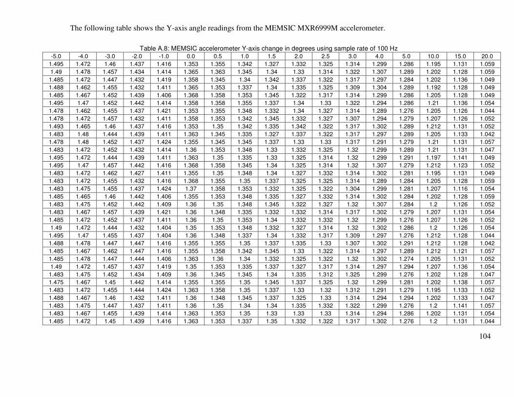
104

The following table shows the Y-axis angle readings from the MEMSIC MXR6999M accelerometer.

Table A.8: MEMSIC accelerometer Y-axis change in degrees using sample rate of 100 Hz

-5.0 -4.0 -3.0 -2.0 -1.0 0.0 0.5 1.0 1.5 2.0 2.5 3.0 4.0 5.0 10.0 15.0 20.0

1.495 1.472 1.46 1.437 1.416 1.353 1.355 1.342 1.327 1.332 1.325 1.314 1.299 1.286 1.195 1.131 1.059

1.49 1.478 1.457 1.434 1.414 1.365 1.363 1.345 1.34 1.33 1.314 1.322 1.307 1.289 1.202 1.128 1.059

1.485 1.472 1.447 1.432 1.419 1.358 1.345 1.34 1.342 1.337 1.322 1.317 1.297 1.284 1.202 1.136 1.049

1.488 1.462 1.455 1.432 1.411 1.365 1.353 1.337 1.34 1.335 1.325 1.309 1.304 1.289 1.192 1.128 1.049

1.485 1.467 1.452 1.439 1.406 1.368 1.358 1.353 1.345 1.322 1.317 1.314 1.299 1.286 1.205 1.128 1.049

1.495 1.47 1.452 1.442 1.414 1.358 1.358 1.355 1.337 1.34 1.33 1.322 1.294 1.286 1.21 1.136 1.054

1.478 1.462 1.455 1.437 1.421 1.353 1.355 1.348 1.332 1.34 1.327 1.314 1.289 1.276 1.205 1.126 1.044

1.478 1.472 1.457 1.432 1.411 1.358 1.353 1.342 1.345 1.332 1.327 1.307 1.294 1.279 1.207 1.126 1.052

1.493 1.465 1.46 1.437 1.416 1.353 1.35 1.342 1.335 1.342 1.322 1.317 1.302 1.289 1.212 1.131 1.052

1.483 1.48 1.444 1.439 1.411 1.363 1.345 1.335 1.327 1.337 1.322 1.317 1.297 1.289 1.205 1.133 1.042

1.478 1.48 1.452 1.437 1.424 1.355 1.345 1.345 1.337 1.33 1.33 1.317 1.291 1.279 1.21 1.131 1.057

1.483 1.472 1.452 1.432 1.414 1.36 1.353 1.348 1.33 1.332 1.325 1.32 1.299 1.289 1.21 1.131 1.047

1.495 1.472 1.444 1.439 1.411 1.363 1.35 1.335 1.33 1.325 1.314 1.32 1.299 1.291 1.197 1.141 1.049

1.495 1.47 1.457 1.442 1.416 1.368 1.358 1.345 1.34 1.325 1.314 1.32 1.307 1.279 1.212 1.123 1.052

1.483 1.472 1.462 1.427 1.411 1.355 1.35 1.348 1.34 1.327 1.332 1.314 1.302 1.281 1.195 1.131 1.049

1.483 1.472 1.455 1.432 1.416 1.368 1.355 1.35 1.337 1.325 1.325 1.314 1.289 1.284 1.205 1.128 1.059

1.483 1.475 1.455 1.437 1.424 1.37 1.358 1.353 1.332 1.325 1.322 1.304 1.299 1.281 1.207 1.116 1.054

1.485 1.465 1.46 1.442 1.406 1.355 1.353 1.348 1.335 1.327 1.332 1.314 1.302 1.284 1.202 1.128 1.059

1.483 1.475 1.452 1.442 1.409 1.36 1.35 1.348 1.345 1.322 1.327 1.32 1.307 1.284 1.2 1.126 1.052

1.483 1.467 1.457 1.439 1.421 1.36 1.348 1.335 1.332 1.332 1.314 1.317 1.302 1.279 1.207 1.131 1.054

1.485 1.472 1.452 1.437 1.411 1.36 1.35 1.353 1.34 1.332 1.332 1.32 1.299 1.276 1.207 1.126 1.052

1.49 1.472 1.444 1.432 1.404 1.35 1.353 1.348 1.332 1.327 1.314 1.32 1.302 1.286 1.2 1.126 1.054

1.495 1.47 1.455 1.437 1.404 1.36 1.348 1.337 1.34 1.332 1.317 1.309 1.297 1.276 1.212 1.128 1.044

1.488 1.478 1.447 1.447 1.416 1.355 1.355 1.35 1.337 1.335 1.33 1.307 1.302 1.291 1.212 1.128 1.042

1.485 1.467 1.462 1.447 1.416 1.355 1.358 1.342 1.345 1.33 1.322 1.314 1.297 1.289 1.212 1.121 1.057

1.485 1.478 1.447 1.444 1.406 1.363 1.36 1.34 1.332 1.325 1.322 1.32 1.302 1.274 1.205 1.131 1.052

1.49 1.472 1.457 1.437 1.419 1.35 1.353 1.335 1.337 1.327 1.317 1.314 1.297 1.294 1.207 1.136 1.054

1.483 1.475 1.452 1.434 1.409 1.36 1.345 1.345 1.34 1.335 1.312 1.325 1.299 1.276 1.202 1.128 1.047

1.475 1.467 1.45 1.442 1.414 1.355 1.355 1.35 1.345 1.337 1.325 1.32 1.299 1.281 1.202 1.138 1.057

1.483 1.472 1.455 1.444 1.424 1.363 1.358 1.35 1.337 1.33 1.32 1.312 1.291 1.279 1.195 1.133 1.052

1.488 1.467 1.46 1.432 1.411 1.36 1.348 1.345 1.337 1.325 1.33 1.314 1.294 1.294 1.202 1.133 1.047

1.483 1.475 1.447 1.437 1.411 1.36 1.35 1.34 1.34 1.335 1.332 1.322 1.299 1.276 1.2 1.141 1.057

1.483 1.467 1.455 1.439 1.414 1.363 1.353 1.35 1.33 1.33 1.33 1.314 1.294 1.286 1.202 1.131 1.054

1.485 1.472 1.45 1.439 1.416 1.363 1.353 1.337 1.35 1.332 1.322 1.317 1.302 1.276 1.2 1.131 1.044

105

1.483 1.467 1.455 1.439 1.411 1.358 1.35 1.342 1.34 1.32 1.322 1.32 1.297 1.284 1.195 1.126 1.054

1.485 1.465 1.444 1.434 1.406 1.36 1.355 1.348 1.342 1.33 1.325 1.314 1.299 1.284 1.202 1.133 1.054

1.483 1.475 1.457 1.434 1.406 1.368 1.345 1.337 1.33 1.327 1.314 1.309 1.307 1.284 1.2 1.131 1.047

1.483 1.472 1.457 1.437 1.406 1.363 1.348 1.35 1.345 1.32 1.325 1.322 1.302 1.289 1.192 1.136 1.044

1.478 1.467 1.447 1.444 1.414 1.36 1.355 1.345 1.332 1.335 1.32 1.322 1.297 1.284 1.202 1.141 1.057

1.493 1.48 1.455 1.437 1.406 1.36 1.355 1.353 1.345 1.33 1.317 1.314 1.289 1.284 1.192 1.133 1.044

1.485 1.467 1.457 1.434 1.421 1.365 1.355 1.345 1.335 1.335 1.327 1.32 1.291 1.289 1.192 1.131 1.049

1.478 1.475 1.447 1.432 1.419 1.363 1.353 1.345 1.342 1.33 1.317 1.322 1.294 1.281 1.207 1.128 1.052

1.485 1.47 1.46 1.442 1.414 1.355 1.345 1.337 1.34 1.322 1.33 1.317 1.294 1.289 1.205 1.126 1.044

1.49 1.467 1.457 1.442 1.421 1.355 1.355 1.337 1.335 1.327 1.322 1.317 1.297 1.281 1.21 1.128 1.047

1.485 1.478 1.452 1.442 1.419 1.355 1.353 1.342 1.342 1.325 1.322 1.317 1.299 1.279 1.2 1.131 1.054

1.483 1.472 1.455 1.437 1.411 1.37 1.353 1.345 1.335 1.325 1.332 1.314 1.302 1.286 1.195 1.133 1.049

1.475 1.462 1.45 1.444 1.419 1.358 1.355 1.345 1.337 1.327 1.33 1.325 1.294 1.284 1.207 1.128 1.042

1.478 1.475 1.46 1.442 1.416 1.355 1.342 1.34 1.335 1.337 1.33 1.309 1.299 1.294 1.207 1.136 1.054

1.488 1.467 1.457 1.432 1.406 1.368 1.353 1.353 1.335 1.325 1.33 1.314 1.309 1.279 1.205 1.123 1.047

1.488 1.478 1.457 1.447 1.414 1.355 1.355 1.345 1.337 1.335 1.322 1.327 1.297 1.289 1.2 1.131 1.057

1.48 1.472 1.455 1.439 1.421 1.355 1.348 1.345 1.337 1.322 1.325 1.309 1.297 1.289 1.202 1.133 1.049

1.48 1.46 1.444 1.444 1.414 1.36 1.348 1.355 1.337 1.325 1.312 1.322 1.302 1.286 1.195 1.131 1.059

1.49 1.47 1.447 1.432 1.406 1.363 1.353 1.34 1.33 1.337 1.317 1.314 1.302 1.284 1.2 1.133 1.044

1.493 1.47 1.455 1.437 1.421 1.37 1.348 1.35 1.335 1.33 1.317 1.32 1.304 1.291 1.197 1.128 1.057

1.488 1.472 1.455 1.442 1.411 1.36 1.342 1.342 1.342 1.327 1.317 1.309 1.294 1.281 1.2 1.133 1.044

1.483 1.472 1.444 1.427 1.416 1.36 1.355 1.35 1.332 1.33 1.317 1.32 1.291 1.289 1.202 1.128 1.049

1.488 1.472 1.444 1.437 1.427 1.363 1.363 1.345 1.345 1.34 1.317 1.317 1.299 1.281 1.202 1.133 1.042

1.485 1.467 1.457 1.434 1.416 1.358 1.353 1.337 1.342 1.337 1.317 1.312 1.291 1.294 1.202 1.136 1.052

1.475 1.472 1.452 1.429 1.416 1.363 1.35 1.337 1.33 1.325 1.322 1.322 1.294 1.284 1.202 1.131 1.052

1.49 1.47 1.457 1.437 1.411 1.35 1.35 1.345 1.335 1.332 1.32 1.317 1.294 1.284 1.212 1.138 1.044

1.485 1.465 1.455 1.437 1.419 1.365 1.363 1.35 1.337 1.335 1.325 1.32 1.299 1.281 1.205 1.131 1.059

1.478 1.478 1.46 1.434 1.409 1.363 1.355 1.337 1.337 1.33 1.317 1.314 1.304 1.276 1.207 1.131 1.049

1.485 1.462 1.457 1.437 1.404 1.365 1.36 1.34 1.33 1.332 1.322 1.312 1.299 1.289 1.21 1.131 1.052

1.478 1.475 1.447 1.437 1.409 1.36 1.358 1.342 1.33 1.332 1.332 1.314 1.294 1.284 1.202 1.138 1.047

1.48 1.467 1.457 1.447 1.414 1.365 1.353 1.34 1.345 1.33 1.325 1.325 1.304 1.284 1.2 1.131 1.057

1.493 1.47 1.46 1.439 1.416 1.35 1.35 1.35 1.345 1.335 1.327 1.314 1.297 1.289 1.202 1.131 1.039

1.483 1.465 1.452 1.427 1.424 1.365 1.348 1.35 1.342 1.32 1.325 1.312 1.294 1.289 1.21 1.131 1.052

1.485 1.472 1.442 1.439 1.419 1.363 1.353 1.342 1.332 1.337 1.325 1.317 1.299 1.279 1.205 1.131 1.044

1.483 1.465 1.455 1.439 1.421 1.353 1.353 1.345 1.345 1.332 1.312 1.325 1.309 1.284 1.2 1.123 1.044

1.488 1.47 1.465 1.437 1.416 1.365 1.345 1.345 1.337 1.327 1.317 1.317 1.307 1.286 1.205 1.131 1.054

1.493 1.472 1.462 1.437 1.427 1.355 1.355 1.34 1.342 1.327 1.325 1.314 1.307 1.289 1.197 1.131 1.039

1.48 1.475 1.452 1.437 1.419 1.365 1.345 1.337 1.34 1.327 1.325 1.312 1.304 1.284 1.197 1.136 1.044

1.488 1.472 1.447 1.434 1.411 1.368 1.355 1.35 1.34 1.327 1.332 1.322 1.291 1.279 1.2 1.123 1.059

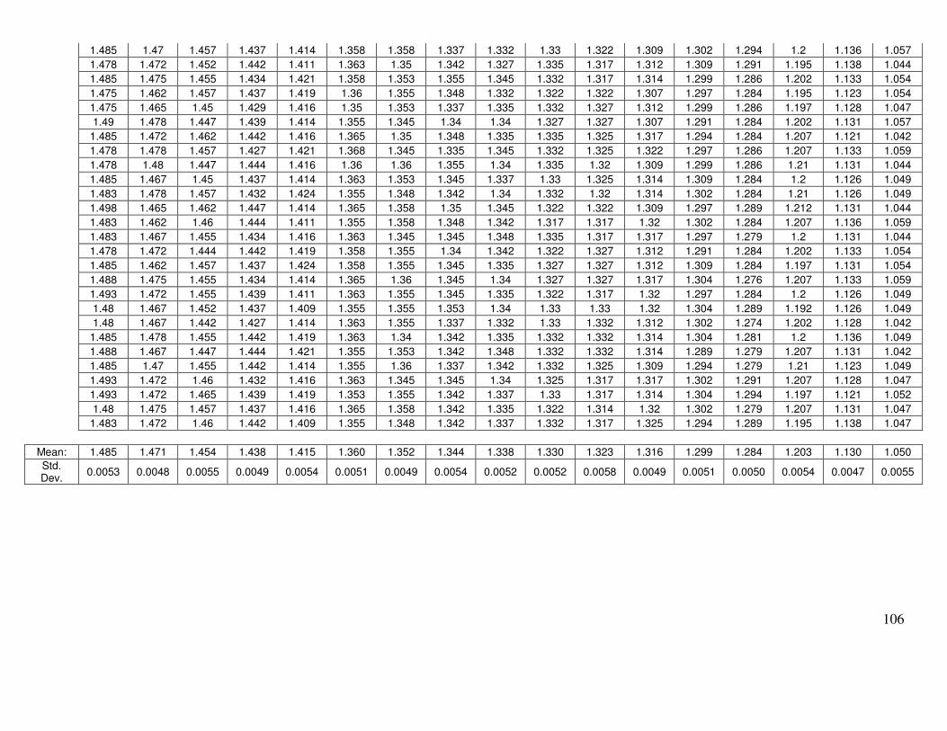
106

1.485 1.47 1.457 1.437 1.414 1.358 1.358 1.337 1.332 1.33 1.322 1.309 1.302 1.294 1.2 1.136 1.057

1.478 1.472 1.452 1.442 1.411 1.363 1.35 1.342 1.327 1.335 1.317 1.312 1.309 1.291 1.195 1.138 1.044

1.485 1.475 1.455 1.434 1.421 1.358 1.353 1.355 1.345 1.332 1.317 1.314 1.299 1.286 1.202 1.133 1.054

1.475 1.462 1.457 1.437 1.419 1.36 1.355 1.348 1.332 1.322 1.322 1.307 1.297 1.284 1.195 1.123 1.054

1.475 1.465 1.45 1.429 1.416 1.35 1.353 1.337 1.335 1.332 1.327 1.312 1.299 1.286 1.197 1.128 1.047

1.49 1.478 1.447 1.439 1.414 1.355 1.345 1.34 1.34 1.327 1.327 1.307 1.291 1.284 1.202 1.131 1.057

1.485 1.472 1.462 1.442 1.416 1.365 1.35 1.348 1.335 1.335 1.325 1.317 1.294 1.284 1.207 1.121 1.042

1.478 1.478 1.457 1.427 1.421 1.368 1.345 1.335 1.345 1.332 1.325 1.322 1.297 1.286 1.207 1.133 1.059

1.478 1.48 1.447 1.444 1.416 1.36 1.36 1.355 1.34 1.335 1.32 1.309 1.299 1.286 1.21 1.131 1.044

1.485 1.467 1.45 1.437 1.414 1.363 1.353 1.345 1.337 1.33 1.325 1.314 1.309 1.284 1.2 1.126 1.049

1.483 1.478 1.457 1.432 1.424 1.355 1.348 1.342 1.34 1.332 1.32 1.314 1.302 1.284 1.21 1.126 1.049

1.498 1.465 1.462 1.447 1.414 1.365 1.358 1.35 1.345 1.322 1.322 1.309 1.297 1.289 1.212 1.131 1.044

1.483 1.462 1.46 1.444 1.411 1.355 1.358 1.348 1.342 1.317 1.317 1.32 1.302 1.284 1.207 1.136 1.059

1.483 1.467 1.455 1.434 1.416 1.363 1.345 1.345 1.348 1.335 1.317 1.317 1.297 1.279 1.2 1.131 1.044

1.478 1.472 1.444 1.442 1.419 1.358 1.355 1.34 1.342 1.322 1.327 1.312 1.291 1.284 1.202 1.133 1.054

1.485 1.462 1.457 1.437 1.424 1.358 1.355 1.345 1.335 1.327 1.327 1.312 1.309 1.284 1.197 1.131 1.054

1.488 1.475 1.455 1.434 1.414 1.365 1.36 1.345 1.34 1.327 1.327 1.317 1.304 1.276 1.207 1.133 1.059

1.493 1.472 1.455 1.439 1.411 1.363 1.355 1.345 1.335 1.322 1.317 1.32 1.297 1.284 1.2 1.126 1.049

1.48 1.467 1.452 1.437 1.409 1.355 1.355 1.353 1.34 1.33 1.33 1.32 1.304 1.289 1.192 1.126 1.049

1.48 1.467 1.442 1.427 1.414 1.363 1.355 1.337 1.332 1.33 1.332 1.312 1.302 1.274 1.202 1.128 1.042

1.485 1.478 1.455 1.442 1.419 1.363 1.34 1.342 1.335 1.332 1.332 1.314 1.304 1.281 1.2 1.136 1.049

1.488 1.467 1.447 1.444 1.421 1.355 1.353 1.342 1.348 1.332 1.332 1.314 1.289 1.279 1.207 1.131 1.042

1.485 1.47 1.455 1.442 1.414 1.355 1.36 1.337 1.342 1.332 1.325 1.309 1.294 1.279 1.21 1.123 1.049

1.493 1.472 1.46 1.432 1.416 1.363 1.345 1.345 1.34 1.325 1.317 1.317 1.302 1.291 1.207 1.128 1.047

1.493 1.472 1.465 1.439 1.419 1.353 1.355 1.342 1.337 1.33 1.317 1.314 1.304 1.294 1.197 1.121 1.052

1.48 1.475 1.457 1.437 1.416 1.365 1.358 1.342 1.335 1.322 1.314 1.32 1.302 1.279 1.207 1.131 1.047

1.483 1.472 1.46 1.442 1.409 1.355 1.348 1.342 1.337 1.332 1.317 1.325 1.294 1.289 1.195 1.138 1.047

Mean: 1.485 1.471 1.454 1.438 1.415 1.360 1.352 1.344 1.338 1.330 1.323 1.316 1.299 1.284 1.203 1.130 1.050

Std. Dev.

0.0053 0.0048 0.0055 0.0049 0.0054 0.0051 0.0049 0.0054 0.0052 0.0052 0.0058 0.0049 0.0051 0.0050 0.0054 0.0047 0.0055

107

Table A.9: Multiple Sensor Test- Raw Data Terminal log file

Date: 3/25/2008 - 9:40:02 AM

-----------------------------------------------

A 2.011764 0.000000

B 1.588235 1.576470

C 1.494117 1.517647

D 1.588235 1.647058

A 2.001176 0.000000

B 1.576470 1.576470

C 1.494117 1.517647

D 1.576470 1.648235

A 2.000000 0.000000

B 1.588235 1.575294

C 1.482352 1.524705

D 1.576470 1.647058

A 2.000000 0.000000

B 1.583529 1.574117

C 1.482352 1.519999

D 1.576470 1.647058

A 2.000000 0.000000

B 1.576470 1.576470

C 1.494117 1.529411

D 1.580000 1.647058

A 2.000000 0.000000

B 1.587058 1.575294

C 1.485882 1.517647

D 1.576470 1.647058

A 2.000000 0.000000

B 1.577647 1.576470

C 1.482352 1.529411

D 1.583529 1.647058

A 2.000000 0.000000

B 1.576470 1.576470

C 1.492941 1.517647

D 1.584705 1.648235

A 2.002352 0.000000

B 1.583529 1.576470

C 1.494117 1.525882

D 1.576470 1.647058

A 2.000000 0.000000

B 1.588235 1.572941

C 1.494117 1.527058

D 1.592941 1.650588

A 2.000000 0.000000

B 1.576470 1.576470

C 1.485882 1.529411

D 1.575294 1.658823

A 2.000000 0.000000

B 1.588235 1.569411

C 1.494117 1.529411

D 1.583529 1.670588

A 2.007058 0.000000

B 1.576470 1.576470

C 1.485882 1.517647

D 1.588235 1.670588

A 2.000000 0.000000

B 1.576470 1.576470

C 1.494117 1.529411

D 1.576470 1.670588

A 2.001176 0.000000

B 1.577647 1.564705

C 1.482352 1.529411

D 1.576470 1.663529

A 2.000000 0.000000

B 1.576470 1.576470

C 1.494117 1.529411

D 1.576470 1.670588

A 2.000000 0.000000

B 1.576470 1.576470

C 1.494117 1.518823

D 1.576470 1.662352

A 2.000000 0.000000

B 1.588235 1.576470

C 1.484705 1.517647

D 1.576470 1.658823

A 2.000000 0.000000

B 1.576470 1.576470

C 1.482352 1.528235

D 1.576470 1.658823

A 2.000000 0.000000

B 1.577647 1.576470

C 1.494117 1.521176

D 1.576470 1.658823

A 2.000000 0.000000

B 1.576470 1.576470

C 1.491764 1.525882

D 1.577647 1.649411

A 2.002352 0.000000

B 1.577647 1.580000

C 1.494117 1.529411

D 1.583529 1.651764

A 2.009411 0.000000

B 1.576470 1.576470

C 1.482352 1.529411

D 1.576470 1.657647

A 2.011764 0.000000

B 1.582352 1.576470

C 1.490588 1.529411

D 1.583529 1.647058

A 2.011764 0.000000

B 1.576470 1.585882

C 1.482352 1.529411

D 1.576470 1.647058

A 2.011764 0.000000

B 1.576470 1.576470

C 1.482352 1.519999

D 1.588235 1.647058

A 2.005882 0.000000

B 1.576470 1.576470

C 1.488235 1.529411

108

D 1.576470 1.647058

A 2.011764 0.000000

B 1.585882 1.585882

C 1.494117 1.528235

D 1.588235 1.647058

A 2.011764 0.000000

B 1.588235 1.576470

C 1.482352 1.529411

D 1.587058 1.647058

A 2.011764 0.000000

B 1.588235 1.576470

C 1.494117 1.529411

D 1.576470 1.647058

A 2.011764 0.000000

B 1.576470 1.576470

C 1.482352 1.529411

D 1.576470 1.657647

A 2.011764 0.000000

B 1.576470 1.576470

C 1.482352 1.529411

D 1.588235 1.658823

A 2.011764 0.000000

B 1.588235 1.576470

C 1.482352 1.529411

D 1.576470 1.651764

A 2.011764 0.000000

B 1.587058 1.576470

C 1.491764 1.529411

D 1.576470 1.667058

A 2.011764 0.000000

B 1.576470 1.576470

C 1.484705 1.529411

D 1.576470 1.658823

A 2.011764 0.000000

B 1.578823 1.576470

C 1.482352 1.529411

D 1.564705 1.670588

A 2.011764 0.000000

B 1.588235 1.576470

C 1.488235 1.529411

D 1.576470 1.682353

A 2.011764 0.000000

B 1.576470 1.585882

C 1.482352 1.529411

D 1.564705 1.689411

B 1.576470 1.576470

C 1.494117 1.529411

D 1.564705 1.705882

B 1.576470 1.576470

C 1.487058 1.529411

D 1.541176 1.729411

B 1.577647 1.576470

C 1.491764 1.529411

D 1.538823 1.764705

B 1.587058 1.576470

C 1.494117 1.529411

D 1.529411 1.847058

B 1.576470 1.576470

C 1.482352 1.529411

D 1.529411 1.929411

B 1.576470 1.576470

C 1.484705 1.529411

D 1.494117 2.011764

B 1.576470 1.576470

C 1.487058 1.529411

D 1.435294 2.141176

B 1.576470 1.575294

C 1.482352 1.529411

D 1.412941 2.211764

B 1.576470 1.576470

C 1.494117 1.529411

D 1.364705 2.294117

B 1.588235 1.576470

C 1.492941 1.529411

D 1.305882 2.467058

B 1.585882 1.576470

C 1.484705 1.529411

D 1.465882 2.808235

B 1.576470 1.576470

C 1.492941 1.529411

D 3.000000 3.000000

B 1.564705 1.564705

C 1.494117 1.529411

D 3.000000 3.000000

B 1.567058 1.552941

C 1.494117 1.529411

D 3.000000 3.000000

B 1.564705 1.564705

C 1.494117 1.529411

B 1.564705 1.552941

C 1.484705 1.529411

G 2.460000 0.000000

G 2.047058 0.000000

B 1.564705 1.564705

C 1.491764 1.541176

G 2.035294 0.000000

B 1.575294 1.567058

C 1.482352 1.541176

G 2.035294 0.000000

B 1.576470 1.576470

C 1.482352 1.550588

G 2.035294 0.000000

B 1.576470 1.588235

C 1.470588 1.552941

B 1.576470 1.588235

C 1.478823 1.563529

G 2.035294 0.000000

B 1.576470 1.602352

C 1.470588 1.572941

G 2.035294 0.000000

B 1.588235 1.611764

C 1.470588 1.576470

109

G 2.035294 0.000000

B 1.577647 1.627058

C 1.458823 1.588235

G 2.035294 0.000000

B 1.600000 1.635294

C 1.505882 1.611764

G 2.035294 0.000000

B 1.611764 1.658823

C 1.635294 1.611764

G 2.035294 0.000000

B 1.607058 1.691764

C 3.000000 0.000000

G 2.035294 0.000000

B 1.623529 1.729411

C 3.000000 0.000000

G 2.036470 0.000000

B 1.647058 1.752941

G 2.035294 0.000000

B 1.670588 1.867058

G 2.035294 0.000000

B 1.717646 1.939999

G 2.035294 0.000000

B 1.676470 2.141176

G 2.035294 0.000000

B 1.601176 2.164705

G 2.035294 0.000000

B 1.471764 2.154117

G 2.047058 0.000000

B 1.341176 2.189411

G 2.042352 0.000000

B 1.251764 2.247058

G 2.047058 0.000000

B 1.012941 2.217647

G 2.035294 0.000000

B 0.636470 2.258823

G 2.035294 0.000000

B 0.282352 2.158823

G 2.047058 0.000000

B 0.143529 2.305882

G 2.047058 0.000000

B 0.000000 2.298823

G 2.047058 0.000000

G 2.035294 0.000000

G 2.047058 0.000000

G 2.047058 0.000000

G 2.047058 0.000000

G 2.047058 0.000000

G 2.047058 0.000000

G 2.048235 0.000000

G 2.047058 0.000000

G 2.043529 0.000000

G 2.047058 0.000000

G 2.047058 0.000000

G 2.044706 0.000000

G 2.047058 0.000000

G 2.048235 0.000000

G 2.047058 0.000000

G 2.047058 0.000000

-----------------------------------------------

Date: 3/27/2008 - 8:58:22 AM

End log file

110

The following table represents the raw data found in Table A.9, only formatted to separate each data

point by identifier. The formatting was performed in Microsoft Excel.

Table A.10: Multiple Tiltmeter Test- Formatted Data

Terminal log file

Date: 3/25/2008 - 9:40:02 AM

-----------------------------------------------

A 2.011764 0 B 1.588235 1.576470 C 1.494117 1.517647 D 1.588235 1.647058

A 2.001176 0 B 1.576470 1.576470 C 1.494117 1.517647 D 1.576470 1.648235

A 2.000000 0 B 1.588235 1.575294 C 1.482352 1.524705 D 1.576470 1.647058

A 2.000000 0 B 1.583529 1.574117 C 1.482352 1.519999 D 1.576470 1.647058

A 2.000000 0 B 1.576470 1.576470 C 1.494117 1.529411 D 1.580000 1.647058

A 2.000000 0 B 1.587058 1.575294 C 1.485882 1.517647 D 1.576470 1.647058

A 2.000000 0 B 1.577647 1.576470 C 1.482352 1.529411 D 1.583529 1.647058

A 2.000000 0 B 1.576470 1.576470 C 1.492941 1.517647 D 1.584705 1.648235

A 2.002352 0 B 1.583529 1.576470 C 1.494117 1.525882 D 1.576470 1.647058

A 2.000000 0 B 1.588235 1.572941 C 1.494117 1.527058 D 1.592941 1.650588

A 2.000000 0 B 1.576470 1.576470 C 1.485882 1.529411 D 1.575294 1.658823

A 2.000000 0 B 1.588235 1.569411 C 1.494117 1.529411 D 1.583529 1.670588

A 2.007058 0 B 1.576470 1.576470 C 1.485882 1.517647 D 1.588235 1.670588

A 2.000000 0 B 1.576470 1.576470 C 1.494117 1.529411 D 1.576470 1.670588

A 2.001176 0 B 1.577647 1.564705 C 1.482352 1.529411 D 1.576470 1.663529

A 2.000000 0 B 1.576470 1.576470 C 1.494117 1.529411 D 1.576470 1.670588

A 2.000000 0 B 1.576470 1.576470 C 1.494117 1.518823 D 1.576470 1.662352

A 2.000000 0 B 1.588235 1.576470 C 1.484705 1.517647 D 1.576470 1.658823

A 2.000000 0 B 1.576470 1.576470 C 1.482352 1.528235 D 1.576470 1.658823

A 2.000000 0 B 1.577647 1.576470 C 1.494117 1.521176 D 1.576470 1.658823

A 2.000000 0 B 1.576470 1.576470 C 1.491764 1.525882 D 1.577647 1.649411

A 2.002352 0 B 1.577647 1.580000 C 1.494117 1.529411 D 1.583529 1.651764

A 2.009411 0 B 1.576470 1.576470 C 1.482352 1.529411 D 1.576470 1.657647

A 2.011764 0 B 1.582352 1.576470 C 1.490588 1.529411 D 1.583529 1.647058

A 2.011764 0 B 1.576470 1.585882 C 1.482352 1.529411 D 1.576470 1.647058

A 2.011764 0 B 1.576470 1.576470 C 1.482352 1.519999 D 1.588235 1.647058

A 2.005882 0 B 1.576470 1.576470 C 1.488235 1.529411 D 1.576470 1.647058

A 2.011764 0 B 1.585882 1.585882 C 1.494117 1.528235 D 1.588235 1.647058

A 2.011764 0 B 1.588235 1.576470 C 1.482352 1.529411 D 1.587058 1.647058

A 2.011764 0 B 1.588235 1.576470 C 1.494117 1.529411 D 1.576470 1.647058

A 2.011764 0 B 1.576470 1.576470 C 1.482352 1.529411 D 1.576470 1.657647

A 2.011764 0 B 1.576470 1.576470 C 1.482352 1.529411 D 1.588235 1.658823

A 2.011764 0 B 1.588235 1.576470 C 1.482352 1.529411 D 1.576470 1.651764

A 2.011764 0 B 1.587058 1.576470 C 1.491764 1.529411 D 1.576470 1.667058

A 2.011764 0 B 1.576470 1.576470 C 1.484705 1.529411 D 1.576470 1.658823

A 2.011764 0 B 1.578823 1.576470 C 1.482352 1.529411 D 1.564705 1.670588

A 2.011764 0 B 1.588235 1.576470 C 1.488235 1.529411 D 1.576470 1.682353

A 2.011764 0 B 1.576470 1.585882 C 1.482352 1.529411 D 1.564705 1.689411

B 1.576470 1.576470 C 1.494117 1.529411 D 1.564705 1.705882

B 1.576470 1.576470 C 1.487058 1.529411 D 1.541176 1.729411

B 1.577647 1.576470 C 1.491764 1.529411 D 1.538823 1.764705

B 1.587058 1.576470 C 1.494117 1.529411 D 1.529411 1.847058

B 1.576470 1.576470 C 1.482352 1.529411 D 1.529411 1.929411

B 1.576470 1.576470 C 1.484705 1.529411 D 1.494117 2.011764

B 1.576470 1.576470 C 1.487058 1.529411 D 1.435294 2.141176

B 1.576470 1.575294 C 1.482352 1.529411 D 1.412941 2.211764

B 1.576470 1.576470 C 1.494117 1.529411 D 1.364705 2.294117

B 1.588235 1.576470 C 1.492941 1.529411 D 1.305882 2.467058

111

B 1.585882 1.576470 C 1.484705 1.529411 D 1.465882 2.808235

B 1.576470 1.576470 C 1.492941 1.529411 D 3.000000 3.000000

B 1.564705 1.564705 C 1.494117 1.529411 D 3.000000 3.000000

B 1.567058 1.552941 C 1.494117 1.529411 D 3.000000 3.000000

B 1.564705 1.564705 C 1.494117 1.529411

B 1.564705 1.552941 C 1.484705 1.529411

B 1.564705 1.564705 C 1.491764 1.541176

B 1.575294 1.567058 C 1.482352 1.541176

B 1.576470 1.576470 C 1.482352 1.550588

B 1.576470 1.588235 C 1.470588 1.552941

B 1.576470 1.588235 C 1.478823 1.563529

B 1.576470 1.602352 C 1.470588 1.572941

B 1.588235 1.611764 C 1.470588 1.576470

B 1.577647 1.627058 C 1.458823 1.588235

B 1.600000 1.635294 C 1.505882 1.611764

B 1.611764 1.658823 C 1.635294 1.611764

B 1.607058 1.691764 C 3.000000 0.000000

B 1.623529 1.729411 C 3.000000 0.000000

B 1.647058 1.752941

B 1.670588 1.867058

B 1.717646 1.939999

B 1.676470 2.141176

B 1.601176 2.164705

B 1.471764 2.154117

B 1.341176 2.189411

B 1.251764 2.247058

B 1.012941 2.217647

B 0.636470 2.258823

B 0.282352 2.158823

B 0.143529 2.305882

B 0.000000 2.298823

-----------------------------------------------

Date: 3/27/2008 - 8:58:22 AM

End log file: Computer Restart

112

APPENDIX B: C CODES

Code Writing Procedure

“Toggle” “Serial Test” “Test ADC”

“Serial Test 2” “Final_A”

113

The process of writing each code to the PIC is described in the following list:

1. Write code in PIC C Compiler

a. Can also use another program such as Microsoft Visual to write the code, as long

as the program uses the C language, not C++.

b. Use attached codes as guides for writing programs. The symbols “//” indicates a

note that does not cause the PIC to read what follows, so follow instructions or

take note as to what trails //.

2. Compile code in PIC C Compiler

a. Compiling the code translates what is written in the C language to a HEX format.

The PIC reads and understands HEX code, but not C, therefore it is important to

compile after any and all changes are made to the code.

3. Use Tiny Bootloader to write compiled code to PIC

a. Attach serial extension, as seen in Figure 4.8, and ensure power to the PIC is on.

b. Select the HEX file using the Browse button in Tiny Bootloader.

c. Press and hold the reset switch on the circuit board.

d. Click the “Write” button in Tiny Bootloader and then release the reset switch on

the circuit board. Tiny Bootloader should then load the program and display a

“Write OK” confirmation.

4. Use Terminal to read serial messages from PIC

a. Terminal will operate using wireless or wired serial methods. Refer to section

4.3- Programming the Circuit Board for more details.

114

APPENDIX B-1: “TOGGLE”

The following code shows the “Toggle” code, written to test the functionality of the PIC,

as described in 4.3- Programming the Circuit Board.

#include <18F6722.h> #ORG 0xFF00, 0xFFFF{} // vsid bootloader //* Set configuration bits in the PIC processor *// /////////////////////////////////////////////////////////////////////////////// #fuses HS, NOPROTECT, NOPUT, NOWDT, NOBROWNOUT, NOLVP, NOCPD, NOWRT #device ADC=8 #use delay (clock=14745600) /* sets appropriate compiler constants */ #use standard_io (a) // IR sensors #use standard_io (b) // LED & Power #use standard_io (d) // Left stepper motor #use standard_io (e) // Right stepper motor #use fixed_io(f_outputs=PIN_F3, PIN_F4, PIN_F5) #use rs232 (BAUD = 9600, XMIT = PIN_C6, RCV = PIN_C7) /////////////////////////////////////////////////////////////////////////////// //* end set configuration bits *// void main(void) { while(1) { output_high(PIN_D1); // Turn camera on delay_ms(2000); //Goes forward for 2 seconds to release arms output_low(PIN_D1); delay_ms(2000); } }

115

APPENDIX B-2: “SERIAL TEST”

The following code shows the “Serial Test” code, written to test the functionality

of the PIC, as described in 4.3- Programming the Circuit Board.

/* This programs sends out a serial message. It can be used as an example of how to do send serial outputs. It also will show if the serial port is working. */ #include <18F6722.h> #ORG 0xFF00, 0xFFFF{} // vsid bootloader #fuses NOWDT,HS, PUT, NOPROTECT, NODEBUG, BROWNOUT, LVP, NOCPD, NOWRT #use delay(clock=14745600) #use rs232(baud=9600,parity=N,xmit=PIN_C6,rcv=PIN_C7,bits=8) void main() { // configure the serial port setup_uart(9600); while(true) { printf("SERIAL TEST\n\r"); delay_ms(1000); } }

116

APPENDIX B-3: “TEST ADC”

The following code shows the “Test ADC” code, written to test the functionality of the

PIC, as described in 4.3- Programming the Circuit Board.

/* This programs reads one of the ADCs and sends the value out on the serial port. It can be used as an example of how to read the analog to digital converters. It also will show if the ADC and serial ports are working. */ #include <18F6722.h> #ORG 0xFF00, 0xFFFF{} // vsid bootloader //* Set configuration bits in the PIC processor *// /////////////////////////////////////////////////////////////////////////////// #fuses HS, NOPROTECT, NOPUT, NOWDT, NOBROWNOUT, NOLVP, NOCPD, NOWRT #device ADC=8 //setup the adc for 8 bit values, can be set as high as 10 #use delay (clock=14745600) /* sets appropriate compiler constants */ #use standard_io (a) #use standard_io (b) #use standard_io (d) #use standard_io (e) #use fixed_io(f_outputs=PIN_F3, PIN_F4, PIN_F5) #use rs232 (BAUD = 115200, XMIT = PIN_C6, RCV = PIN_C7) /////////////////////////////////////////////////////////////////////////////// //* end set configuration bits *// //****************************************************************** //Function name: initialization //Purpose: Initializes motors, timers, interrupts // and adc. //Precondition: void //Postcondition: void //****************************************************************** void initialization() { //* Initializes ADC *// setup_adc(ADC_CLOCK_INTERNAL); setup_adc_ports(ALL_ANALOG); //use all adc pins as adcs (can set some as digital I/O if needed }

117

//****************************************************************** //Function name: main //Purpose: 1. Initializing. // 2. Main sensing loop. //Precondition: void //Postcondition: void //****************************************************************** void main(void) { initialization(); while(1) { //keep running this loop until the PIC is turned off int32 sum_x = 0; int32 sum_y = 0; set_adc_channel(0); // delay_us(10); //delay required after setting adc_channel sum_x = sum_x + read_ADC(); set_adc_channel(1); delay_us(10); sum_y = sum_y + read_ADC(); // send out sensor_value in ascii over serial printf("The sum_x and sum_y ADC value is \n\r %u, and %u.\n\r", sum_x, sum_y); delay_ms(2000); } }

118

APPENDIX B-4: “SERIAL TEST 2”

The following code shows the “Serial Test 2” code, written to test the functionality of the

PIC, as well as the wireless capabilities of the XBee, as described in 4.3- Programming the

Circuit Board.

/* This programs sends out a serial message. It can be used as an example of how to do send serial outputs. It also will show if the serial port is working. */ #include <18F6722.h> #ORG 0xFF00, 0xFFFF{} // vsid bootloader #fuses NOWDT,HS, PUT, NOPROTECT, NODEBUG, BROWNOUT, LVP, NOCPD, NOWRT #use delay(clock=14745600) #use rs232(baud=9600,parity=N,xmit=PIN_G2,rcv=PIN_G1,bits=8) void main() { // configure the serial port //setup_uart(9600); while(true) { printf("SERIAL TEST\n\r"); delay_ms(1000); } }

119

APPENDIX B-5: “FINAL_A”

The following code shows the “Final_A” code, written for the tiltmeters upon completion

of the designing process, as described in 4.3- Programming the Circuit Board. This code was

written to each of the sensors installed at the Fairfax Luck Stone mine, with the differentiation of

an identifier: “Final_A” output the identifier A, and “Final_B” outputs the identifier B, etc.

/* This program reads one of the ADC at 100 Hz and sends the data out on the serial port. It is an example of how to use interrupts */ #include <18F6722.h> #ORG 0xFF00, 0xFFFF{} // vsid bootloader //* Set configuration bits in the PIC processor *// /////////////////////////////////////////////////////////////////////////////// #fuses HS, NOPROTECT, NOPUT, NOWDT, NOBROWNOUT, NOLVP, NOCPD, NOWRT #device ADC=8 #use delay (clock=14745600) /* sets appropriate compiler constants */ #use standard_io (a) // IR sensors #use standard_io (b) // LED & Power #use standard_io (d) // Left stepper motor #use standard_io (e) // Right stepper motor #use fixed_io(f_outputs=PIN_F3, PIN_F4, PIN_F5) #use rs232 (BAUD = 9600, XMIT = PIN_G2, RCV = PIN_G1) float sum_x = 0; float sum_y = 0; int8 count = 0; int8 i = 0; int8 j = 0; float Avg_x = 0; float Avg_y = 0; /////////////////////////////////////////////////////////////////////////////// //* end set configuration bits *// //****************************************************************** //Function name: movement //Purpose: Executes when interrupt timer1 overflows.

120

//Precondition: void //Postcondition: void //****************************************************************** #int_timer1 void adc_read() { delay_ms(5000); while(true) { set_timer1(0x2100); // sets timer interrupt at 100 Hz // Clock divisior is 4608 = 0x1200, but order must be flipped to 0x2100(weird compiler bug) set_adc_channel(0); // delay_us(10); //delay required after setting adc_channel {for (i=0;i<=9;++i) sum_x = sum_x + read_ADC();} set_adc_channel(1); delay_us(10); //delay required after setting adc_channel {for (j=0;j<=9;++j) sum_y = sum_y + read_ADC();} Avg_x = sum_x*3/255/i; //(using conversion factor of 3/255 [Voltage/((2^8bits)-1)]) Avg_y = sum_y*3/255/j; {// send out X & Y voltages in ascii over serial port printf("A, %f, %f.\n\r", Avg_x, Avg_y); delay_ms(1800000);} //1800000 ms = 30 minutes. signal will be transmitted every 30 minutes sum_x = sum_y = Avg_x = Avg_y = 0; }} //****************************************************************** //Function name: initialization //Purpose: Initializes motors, timers, interrupts // and adc. //Precondition: void //Postcondition: void //****************************************************************** void initialization() { //* Initializes ADC *// setup_adc(ADC_CLOCK_INTERNAL); setup_adc_ports(AN0_TO_AN9); //* Timer setups *// setup_timer_1(T1_internal | T1_DIV_BY_8); // Timer speed is Fosc/4/T1_DIV_BY_8 = 14.7456 MHz / 4 / 8 = 460.8 kHz } //******************************************************************

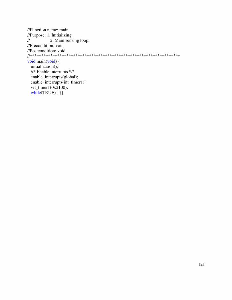
121

//Function name: main //Purpose: 1. Initializing. // 2. Main sensing loop. //Precondition: void //Postcondition: void //****************************************************************** void main(void) { initialization(); //* Enable interrupts *// enable_interrupts(global); enable_interrupts(int_timer1); set_timer1(0x2100); while(TRUE) {}}

122

APPENDIX C: CIRCUIT BOARD COMPONENTS

Initial Prototype Component List

Final Revised Component List Prototype Board Cost Analysis Revised Board Cost Analysis

123

Table C.1: Initial Prototype Component List Part Value Device Package Description Company Part #

B1 BAT_CR2032 BAT_CR2032 2032SM Battery Digi-Key BA2032-ND

C1 0.1 µF CAP-0805 805 Capacitors Digi-Key 399-1168-1-ND

C2 1 µF CAP-0805 805 Capacitors Digi-Key 399-1284-1-ND


C7 22 pF CAP-0603 603 Capacitors Digi-Key 399-1053-1-ND













C21 1µF CAP-0805 805 Capacitors Digi-Key 399-1284-1-ND

C22 1µF CAP-0805 805 Capacitors Digi-Key 399-1284-1-ND

CN3 CN-JST_5 CN-JST_5 JST5 Connector Digi-Key 455-1707-ND

D1-IN IN LED-1206 1206-POL Diode Digi-Key 160-1456-1-ND

D2-OUT OUT LED-1206 1206-POL Diode Digi-Key 160-1456-1-ND

D3-ASSOC ASSOC LED-1206 1206-POL Diode Digi-Key 160-1405-1-ND

D5 PWM1 LED-1206 1206-POL Diode Digi-Key 160-1405-1-ND

D6 DSR/DCD LED-1206 1206-POL Diode Digi-Key 160-1406-1-ND

JP1 JP-3 JP-3 JP3 Jumper Digi-Key WM6536-ND



JP4-COORD COORD JP-2 JP2 Jumper Digi-Key WM6536-ND

M2 XBee XBee XBee XBee MaxStream XB24-BWIT-004

MEMSIC 1000mv/g MXR6999M MXR6999M Accelerometer MEMSIC MXR6999M

Q2 PNP MMBT3906 SOT-23 Transistor Digi-Key MMBT3906FSCT-ND




R2 10k RES-0805 805 Resistor Digi-Key RHM10KARCT-ND



R16 470 RES-0805 805 Resistor Digi-Key RHM470ARCT-ND








R26 220 RES-0805 805 Resistor Digi-Key RHM220ACT-ND

R27 220 RES-0805 805 Resistor Digi-Key RHM220ACT-ND

SERIAL CN-JST_3 CN-JST_3 JST3 Serial Digi-Key 455-1705-ND

SERIAL1 CN-JST_3 CN-JST_3 JST3 Serial Digi-Key 455-1705-ND

SW1 SW_B3S-1000 SW_B3S-1000 B3S-1000 Switch Digi-Key SW415-ND

U2 PIC18F6722 PIC18F6722 LQFP-64 Processor Microchip PIC18F6722-I/PT

U4 MAX3232 MAX3232 SOIC-16 Driver/Receiver Texas Inst. MAX3232CDR

Y2 18pF XTAL-CS10 CS10 Crystals Digi-Key 300-8094-1-ND

124

Table C.2: Final Revised Component List

Part Value Device Package Description Company Part #

BAT AA*2_-_3V AA_HOUSING AA_HOUSING Battery Digi-Key SBH-321AS-ND

C01 0.1 uF CAP-0603 603 Capacitors Digi-Key 399-1096-1-ND

C02 1 uF CAP-0805 805 Capacitors Digi-Key 399-1284-1-ND















C17 1uF CAP-0805 805 Capacitors Digi-Key 399-1284-1-ND

C18 1uF CAP-0805 805 Capacitors Digi-Key 399-1284-1-ND

CN3 CN-JST_5 CN-JST_5 JST5 Connector Digi-Key 455-1707-ND



2 XBee XBee XBee MaxStream MaxStream XB24-BWIT-004

MEMSIC Accelerometer MXR6999M MXR6999M Accelerometer MEMSIC MXR6999M

Q1 Q_MMBT3906 Q_MMBT3906 SOT-23 Transistor Digi-Key MMBT3906FSCT-ND




R01 10K RES-0805 805 Resistors Digi-Key RHM10KARCT-ND

R02 10k RES-0805 805 Resistors Digi-Key RHM10KARCT-ND



R05 470 RES-0805 805 Resistors Digi-Key RHM470ARCT-ND



R08 470 RES-0805 805 Resistors Digi-Key RHM470ARCT-ND

RCV RCV LED-1206 1206-POL Diode Digi-Key 160-1456-1-ND

SERIAL-PIC CN-JST_3 CN-JST_3 JST3 Serial Digi-Key 455-1705-ND

SERIAL1 CN-JST_3 CN-JST_3 JST3 Serial Digi-Key 455-1705-ND

SND SND LED-1206 1206-POL Diode Digi-Key 160-1456-1-ND

SW1 SW_B3S-1000 SW_B3S-1000 B3S-1000 Switch Digi-Key SW415-ND

U2 PIC18F6722 PIC18F6722 LQFP-64 Processor Microchip PIC18F6722-I/PT

U4 MAX3232 MAX3232 SOIC-16 Driver/Receiver Texas Inst. MAX3232CDR

Y2 18 pF XTAL-CS10 CS10 Crystals Digi-Key 300-8094-1-ND

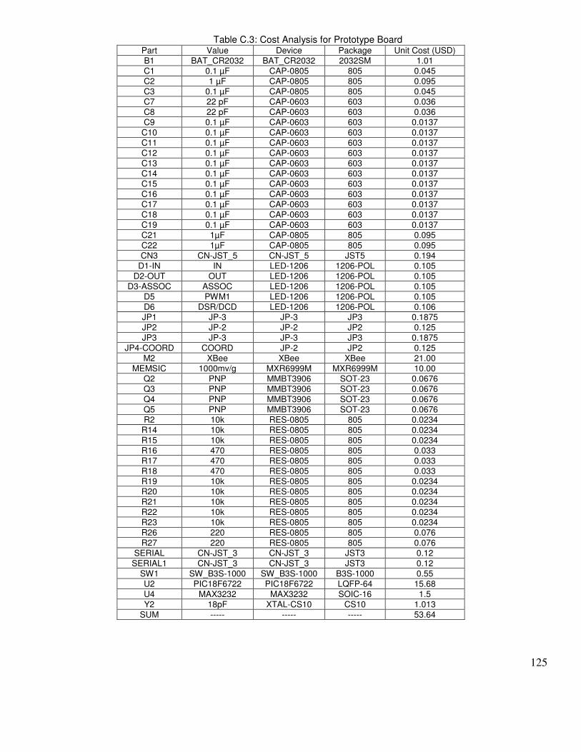
125

Table C.3: Cost Analysis for Prototype Board Part Value Device Package Unit Cost (USD) B1 BAT_CR2032 BAT_CR2032 2032SM 1.01 C1 0.1 µF CAP-0805 805 0.045 C2 1 µF CAP-0805 805 0.095 C3 0.1 µF CAP-0805 805 0.045 C7 22 pF CAP-0603 603 0.036 C8 22 pF CAP-0603 603 0.036 C9 0.1 µF CAP-0603 603 0.0137

C10 0.1 µF CAP-0603 603 0.0137 C11 0.1 µF CAP-0603 603 0.0137 C12 0.1 µF CAP-0603 603 0.0137 C13 0.1 µF CAP-0603 603 0.0137 C14 0.1 µF CAP-0603 603 0.0137 C15 0.1 µF CAP-0603 603 0.0137 C16 0.1 µF CAP-0603 603 0.0137 C17 0.1 µF CAP-0603 603 0.0137 C18 0.1 µF CAP-0603 603 0.0137 C19 0.1 µF CAP-0603 603 0.0137 C21 1µF CAP-0805 805 0.095 C22 1µF CAP-0805 805 0.095 CN3 CN-JST_5 CN-JST_5 JST5 0.194

D1-IN IN LED-1206 1206-POL 0.105 D2-OUT OUT LED-1206 1206-POL 0.105

D3-ASSOC ASSOC LED-1206 1206-POL 0.105 D5 PWM1 LED-1206 1206-POL 0.105 D6 DSR/DCD LED-1206 1206-POL 0.106 JP1 JP-3 JP-3 JP3 0.1875 JP2 JP-2 JP-2 JP2 0.125 JP3 JP-3 JP-3 JP3 0.1875

JP4-COORD COORD JP-2 JP2 0.125 M2 XBee XBee XBee 21.00

MEMSIC 1000mv/g MXR6999M MXR6999M 10.00 Q2 PNP MMBT3906 SOT-23 0.0676 Q3 PNP MMBT3906 SOT-23 0.0676 Q4 PNP MMBT3906 SOT-23 0.0676 Q5 PNP MMBT3906 SOT-23 0.0676 R2 10k RES-0805 805 0.0234

R14 10k RES-0805 805 0.0234 R15 10k RES-0805 805 0.0234 R16 470 RES-0805 805 0.033 R17 470 RES-0805 805 0.033 R18 470 RES-0805 805 0.033 R19 10k RES-0805 805 0.0234 R20 10k RES-0805 805 0.0234 R21 10k RES-0805 805 0.0234 R22 10k RES-0805 805 0.0234 R23 10k RES-0805 805 0.0234 R26 220 RES-0805 805 0.076 R27 220 RES-0805 805 0.076

SERIAL CN-JST_3 CN-JST_3 JST3 0.12 SERIAL1 CN-JST_3 CN-JST_3 JST3 0.12

SW1 SW_B3S-1000 SW_B3S-1000 B3S-1000 0.55 U2 PIC18F6722 PIC18F6722 LQFP-64 15.68 U4 MAX3232 MAX3232 SOIC-16 1.5 Y2 18pF XTAL-CS10 CS10 1.013

SUM ----- ----- ----- 53.64

126

Table C.4: Cost Analysis for Revised Board Part Value Device Package Unit Cost

BAT AA*2_-_3V AA_HOUSING AA_HOUSING 0.70

C01 0.1 uF CAP-0603 603 0.0137

C02 1 uF CAP-0805 805 0.045

C03 0.1 uF CAP-0603 603 0.0137

C04 22 pF CAP-0603 603 0.036

C05 22 pF CAP-0603 603 0.036

C06 0.1 uF CAP-0603 603 0.0137

C07 0.1 uF CAP-0603 603 0.0137

C08 0.1 uF CAP-0603 603 0.0137

C09 0.1 uF CAP-0603 603 0.0137

C10 0.1 uF CAP-0603 603 0.0137

C11 0.1 uF CAP-0603 603 0.0137

C12 0.1 uF CAP-0603 603 0.0137

C13 0.1 uF CAP-0603 603 0.0137

C14 0.1 uF CAP-0603 603 0.0137

C15 0.1 uF CAP-0603 603 0.0137

C16 0.1 uF CAP-0603 603 0.0137

C17 1uF CAP-0805 805 0.045

C18 1uF CAP-0805 805 0.045

CN3 CN-JST_5 CN-JST_5 JST5 0.194

JP1 JP-3 JP-3 JP3 0.1875

JP2 JP-3 JP-3 JP3 0.1875

M2 XBee XBee XBee 21.00

MEMSIC Accelerometer MXR6999M MXR6999M 10.00

Q1 Q_MMBT3906 Q_MMBT3906 SOT-23 0.0676

Q2 Q_MMBT3906 Q_MMBT3906 SOT-23 0.0676

Q3 Q_MMBT3906 Q_MMBT3906 SOT-23 0.0676

Q4 Q_MMBT3906 Q_MMBT3906 SOT-23 0.0676

R01 10K RES-0805 805 0.0234

R02 10k RES-0805 805 0.0234

R03 10k RES-0805 805 0.0234

R04 10k RES-0805 805 0.0234

R05 470 RES-0805 805 0.033

R06 10k RES-0805 805 0.0234

R07 10k RES-0805 805 0.0234

R08 470 RES-0805 805 0.033

RCV RCV LED-1206 1206-POL 0.105

SERIAL-PIC CN-JST_3 CN-JST_3 JST3 0.12

SERIAL1 CN-JST_3 CN-JST_3 JST3 0.12

SND SND LED-1206 1206-POL 0.105

SW1 SW_B3S-1000 SW_B3S-1000 B3S-1000 0.55

U2 PIC18F6722 PIC18F6722 LQFP-64 15.68

U4 MAX3232 MAX3232 SOIC-16 1.5

Y2 18 pF XTAL-CS10 CS10 1.013

SUM ----- ----- ----- 52.32

127

APPENDIX D: FIELD TEST DATA

Formatted Data from Mine

128

The following table includes formatted data from the site test beginning on Tuesday April 1, 2008 and ending on Monday April 7, 2008. The

“Estimated Time” column was extrapolated using a recorded initial time of each tiltmeter’s first transmission, and adding 30 minutes for the

following time. A cell containing “XXXXX” was not used for analysis purposes, as the measurement recorded was either before or after the tiltmeter

was securely fastened or removed from its permanent position. Those measurements adjacent to cells containing “XXXXX” were severe outliers

when plotting the data.

Table D.1: Formatted Data from Test Mine Site Terminal log file

Date: 4/1/2008 - 1:08:35 PM -----------------------------------------------

X- axis Y- axis Estimated Time X- axis Y- axis Estimated Time X- axis Y- axis Estimated Time B 1.505882 1.447058 XXXXX C 1.470588 1.472941 XXXXX

A 1.447058 1.494117 XXXXX B 1.304705 1.435294 XXXXX C 1.399999 1.482352 XXXXX A 1.482352 1.576470 4/1/2008 14:05 B 1.294117 1.458823 XXXXX C 1.388235 1.470588 4/1/2008 14:05 A 1.494117 1.558823 14:35 B 1.288235 1.467058 4/1/2008 14:23 C 1.389411 1.470588 14:35 A 1.494117 1.552941 15:05 B 1.282352 1.460000 14:53 C 1.399999 1.482352 15:05 A 1.482352 1.542353 15:35 B 1.282352 1.460000 15:23 C 1.399999 1.470588 15:35 A 1.482352 1.545882 16:05 B 1.294117 1.458823 15:53 C 1.399999 1.470588 16:05 A 1.482352 1.541176 16:35 B 1.282352 1.458823 16:23 C 1.399999 1.470588 16:35 A 1.470588 1.539999 17:05 B 1.291764 1.458823 16:53 C 1.399999 1.471764 17:05 A 1.470588 1.529411 17:35 B 1.291764 1.460000 17:23 C 1.399999 1.470588 17:35 A 1.470588 1.529411 18:05 B 1.294117 1.470588 17:53 C 1.399999 1.470588 18:05 A 1.469411 1.529411 18:35 B 1.294117 1.462352 18:23 C 1.399999 1.474117 18:35 A 1.469411 1.529411 19:05 B 1.294117 1.470588 18:53 C 1.399999 1.470588 19:05 A 1.470588 1.529411 19:35 B 1.294117 1.471764 19:23 C 1.399999 1.471764 19:35 A 1.470588 1.529411 20:05 B 1.294117 1.470588 19:53 C 1.399999 1.470588 20:05 A 1.462352 1.529411 20:35 B 1.294117 1.470588 20:23 C 1.399999 1.474117 20:35 A 1.458823 1.529411 21:05 B 1.294117 1.469411 20:53 C 1.391764 1.482352 21:05 A 1.470588 1.529411 21:35 B 1.294117 1.470588 21:23 C 1.394117 1.470588 21:35 A 1.465882 1.529411 22:05 B 1.294117 1.471764 21:53 C 1.399999 1.482352 22:05 A 1.470588 1.529411 22:35 B 1.294117 1.469411 22:23 C 1.399999 1.482352 22:35 A 1.470588 1.529411 23:05 B 1.294117 1.470588 22:53 C 1.399999 1.470588 23:05 A 1.470588 1.529411 23:35 B 1.295294 1.468235 23:23 C 1.399999 1.482352 23:35 A 1.470588 1.529411 4/2/2008 0:05 B 1.294117 1.469411 23:53 C 1.399999 1.481176 4/2/2008 0:05 A 1.470588 1.529411 0:35 B 1.294117 1.470588 4/2/2008 0:23 C 1.399999 1.482352 0:35 A 1.469411 1.529411 1:05 B 1.295294 1.471764 0:53 C 1.388235 1.482352 1:05 A 1.464705 1.529411 1:35 B 1.295294 1.470588 1:23 C 1.399999 1.482352 1:35 A 1.465882 1.529411 2:05 B 1.295294 1.469411 1:53 C 1.399999 1.482352 2:05 A 1.470588 1.529411 2:35 B 1.294117 1.471764 2:23 C 1.399999 1.482352 2:35

129

A 1.462352 1.528235 3:05 B 1.295294 1.470588 2:53 C 1.399999 1.482352 3:05 A 1.470588 1.521176 3:35 B 1.298823 1.465882 3:23 C 1.388235 1.482352 3:35 A 1.470588 1.529411 4:05 B 1.294117 1.470588 3:53 C 1.398823 1.482352 4:05 A 1.468235 1.528235 4:35 B 1.294117 1.470588 4:23 C 1.388235 1.483529 4:35 A 1.458823 1.529411 5:05 B 1.295294 1.471764 4:53 C 1.399999 1.482352 5:05 A 1.467058 1.518823 5:35 B 1.294117 1.470588 5:23 C 1.392941 1.482352 5:35 A 1.465882 1.527058 6:05 B 1.294117 1.470588 5:53 C 1.399999 1.482352 6:05 A 1.458823 1.523529 6:35 B 1.296470 1.465882 6:23 C 1.399999 1.482352 6:35 A 1.458823 1.541176 7:05 B 1.297647 1.470588 6:53 C 1.395294 1.483529 7:05 A 1.460000 1.529411 7:35 B 1.294117 1.470588 7:23 C 1.396470 1.482352 7:35 A 1.467058 1.530588 8:05 B 1.294117 1.470588 7:53 C 1.399999 1.482352 8:05 A 1.470588 1.531764 8:35 B 1.294117 1.470588 8:23 C 1.392941 1.482352 8:35 A 1.460000 1.517647 9:05 B 1.301176 1.470588 8:53 C 1.397647 1.482352 9:05 A 1.470588 1.529411 9:35 B 1.294117 1.469411 9:23 C 1.389411 1.482352 9:35 A 1.470588 1.535294 10:05 B 1.294117 1.470588 9:53 C 1.399999 1.482352 10:05 A 1.482352 1.541176 10:35 B 1.294117 1.470588 10:23 C 1.399999 1.494117 10:35 A 1.482352 1.552941 11:05 B 1.297647 1.460000 10:53 C 1.399999 1.482352 11:05 A 1.470588 1.529411 11:35 B 1.294117 1.458823 11:23 C 1.411764 1.482352 11:35 A 1.488235 1.564705 12:05 B 1.294117 1.458823 11:53 C 1.422353 1.484705 12:05 A 1.482352 1.541176 12:35 B 1.282352 1.454117 12:23 C 1.414117 1.482352 12:35 A 1.494117 1.541176 13:05 B 1.294117 1.458823 12:53 C 1.409411 1.482352 13:05 A 1.494117 1.562353 13:35 B 1.294117 1.458823 13:23 C 1.399999 1.471764 13:35 A 1.482352 1.564705 14:05 B 1.294117 1.458823 13:53 C 1.399999 1.474117 14:05 A 1.482352 1.541176 14:35 B 1.294117 1.458823 14:23 C 1.388235 1.470588 14:35 A 1.485882 1.552941 15:05 B 1.294117 1.460000 14:53 C 1.399999 1.482352 15:05 A 1.482352 1.541176 15:35 B 1.294117 1.458823 15:23 C 1.399999 1.470588 15:35 A 1.471764 1.541176 16:05 B 1.294117 1.461176 15:53 C 1.399999 1.470588 16:05 A 1.482352 1.541176 16:35 B 1.294117 1.460000 16:23 C 1.399999 1.481176 16:35 A 1.470588 1.529411 17:05 B 1.295294 1.461176 16:53 C 1.399999 1.481176 17:05 A 1.470588 1.529411 17:35 B 1.292941 1.461176 17:23 C 1.399999 1.482352 17:35 A 1.470588 1.541176 18:05 B 1.294117 1.461176 17:53 C 1.389411 1.482352 18:05 A 1.470588 1.529411 18:35 B 1.294117 1.468235 18:23 C 1.399999 1.481176 18:35 A 1.470588 1.529411 19:05 B 1.294117 1.464705 18:53 C 1.390588 1.482352 19:05 A 1.458823 1.529411 19:35 B 1.295294 1.470588 19:23 C 1.394117 1.482352 19:35 A 1.467058 1.529411 20:05 B 1.295294 1.470588 19:53 C 1.399999 1.482352 20:05 A 1.463529 1.529411 20:35 B 1.294117 1.470588 20:23 C 1.399999 1.482352 20:35 A 1.458823 1.521176 21:05 B 1.295294 1.465882 20:53 C 1.388235 1.481176 21:05 A 1.464705 1.529411 21:35 B 1.294117 1.470588 21:23 C 1.399999 1.482352 21:35 A 1.470588 1.528235 22:05 B 1.295294 1.470588 21:53 C 1.388235 1.482352 22:05 A 1.462352 1.529411 22:35 B 1.294117 1.470588 22:23 C 1.398823 1.482352 22:35 A 1.465882 1.529411 23:05 B 1.297647 1.470588 22:53 C 1.388235 1.483529 23:05 A 1.469411 1.529411 23:35 B 1.305882 1.470588 23:23 C 1.399999 1.482352 23:35 A 1.460000 1.529411 4/3/2008 0:05 B 1.294117 1.470588 23:53 C 1.390588 1.482352 4/3/2008 0:05

130

A 1.470588 1.521176 0:35 B 1.301176 1.470588 4/3/2008 0:23 C 1.399999 1.482352 0:35 A 1.460000 1.519999 1:05 B 1.297647 1.470588 0:53 C 1.399999 1.483529 1:05 A 1.470588 1.517647 1:35 B 1.296470 1.470588 1:23 C 1.399999 1.483529 1:35 A 1.461176 1.524705 2:05 B 1.303529 1.470588 1:53 C 1.396470 1.482352 2:05 A 1.462352 1.517647 2:35 B 1.298823 1.470588 2:23 C 1.399999 1.482352 2:35 A 1.467058 1.517647 3:05 B 1.294117 1.470588 2:53 C 1.394117 1.482352 3:05 A 1.470588 1.523529 3:35 B 1.298823 1.470588 3:23 C 1.398823 1.482352 3:35 A 1.458823 1.519999 4:05 B 1.294117 1.470588 3:53 C 1.399999 1.482352 4:05 A 1.470588 1.525882 4:35 B 1.305882 1.470588 4:23 C 1.388235 1.482352 4:35 A 1.458823 1.529411 5:05 B 1.295294 1.470588 4:53 C 1.388235 1.484705 5:05 A 1.460000 1.522353 5:35 B 1.303529 1.470588 5:23 C 1.388235 1.482352 5:35 A 1.468235 1.519999 6:05 B 1.294117 1.470588 5:53 C 1.399999 1.482352 6:05 A 1.470588 1.517647 6:35 B 1.305882 1.470588 6:23 C 1.399999 1.482352 6:35 A 1.460000 1.517647 7:05 B 1.305882 1.470588 6:53 C 1.397647 1.482352 7:05 A 1.458823 1.521176 7:35 B 1.296470 1.470588 7:23 C 1.399999 1.482352 7:35 A 1.470588 1.517647 8:05 B 1.305882 1.470588 7:53 C 1.399999 1.483529 8:05 A 1.470588 1.517647 8:35 B 1.297647 1.470588 8:23 C 1.399999 1.482352 8:35 A 1.470588 1.518823 9:05 B 1.294117 1.470588 8:53 C 1.399999 1.482352 9:05 A 1.470588 1.529411 9:35 B 1.305882 1.470588 9:23 C 1.399999 1.482352 9:35 A 1.470588 1.529411 10:05 B 1.294117 1.470588 9:53 C 1.389411 1.482352 10:05 A 1.470588 1.517647 10:35 B 1.294117 1.470588 10:23 C 1.399999 1.482352 10:35 A 1.468235 1.529411 11:05 B 1.294117 1.470588 10:53 C 1.399999 1.482352 11:05 A 1.465882 1.541176 11:35 B 1.295294 1.470588 11:23 C 1.399999 1.482352 11:35 A 1.470588 1.510588 12:05 B 1.294117 1.470588 11:53 C 1.399999 1.483529 12:05 A 1.470588 1.541176 12:35 B 1.294117 1.470588 12:23 C 1.399999 1.482352 12:35 A 1.470588 1.530588 13:05 B 1.294117 1.470588 12:53 C 1.398823 1.482352 13:05 A 1.470588 1.528235 13:35 B 1.294117 1.469411 13:23 C 1.399999 1.482352 13:35 A 1.460000 1.521176 14:05 B 1.296470 1.464705 13:53 C 1.398823 1.482352 14:05 A 1.481176 1.517647 14:35 B 1.305882 1.470588 14:23 C 1.399999 1.482352 14:35 A 1.470588 1.525882 15:05 B 1.294117 1.470588 14:53 C 1.398823 1.482352 15:05 A 1.470588 1.517647 15:35 B 1.305882 1.470588 15:23 C 1.398823 1.489411 15:35 A 1.470588 1.529411 16:05 B 1.295294 1.470588 15:53 C 1.399999 1.482352 16:05 A 1.470588 1.529411 16:35 B 1.298823 1.470588 16:23 C 1.399999 1.482352 16:35 A 1.470588 1.517647 17:05 B 1.294117 1.470588 16:53 C 1.389411 1.482352 17:05 A 1.458823 1.523529 17:35 B 1.296470 1.470588 17:23 C 1.399999 1.482352 17:35 A 1.470588 1.517647 18:05 B 1.302352 1.470588 17:53 C 1.397647 1.482352 18:05 A 1.470588 1.519999 18:35 B 1.301176 1.470588 18:23 C 1.399999 1.482352 18:35 A 1.470588 1.518823 19:05 B 1.294117 1.470588 18:53 C 1.399999 1.487058 19:05 A 1.470588 1.529411 19:35 B 1.294117 1.470588 19:23 C 1.389411 1.482352 19:35 A 1.470588 1.517647 20:05 B 1.295294 1.470588 19:53 C 1.399999 1.482352 20:05 A 1.469411 1.517647 20:35 B 1.295294 1.470588 20:23 C 1.399999 1.482352 20:35 A 1.469411 1.519999 21:05 B 1.294117 1.470588 20:53 C 1.397647 1.483529 21:05 A 1.470588 1.518823 21:35 B 1.297647 1.470588 21:23 C 1.399999 1.482352 21:35

131

A 1.470588 1.518823 22:05 B 1.301176 1.470588 21:53 C 1.399999 1.483529 22:05 A 1.470588 1.519999 22:35 B 1.305882 1.470588 22:23 C 1.388235 1.482352 22:35 A 1.470588 1.521176 23:05 B 1.305882 1.470588 22:53 C 1.399999 1.482352 23:05 A 1.470588 1.527058 23:35 B 1.305882 1.470588 23:23 C 1.399999 1.482352 23:35 A 1.458823 1.517647 4/4/2008 0:05 B 1.305882 1.458823 23:53 C 1.399999 1.482352 4/4/2008 0:05 A 1.465882 1.517647 0:35 B 1.303529 1.460000 4/4/2008 0:23 C 1.399999 1.482352 0:35 A 1.464705 1.517647 1:05 B 1.305882 1.468235 0:53 C 1.396470 1.482352 1:05 A 1.470588 1.523529 1:35 B 1.294117 1.470588 1:23 C 1.399999 1.482352 1:35 A 1.470588 1.517647 2:05 B 1.305882 1.470588 1:53 C 1.399999 1.482352 2:05 A 1.468235 1.518823 2:35 B 1.305882 1.470588 2:23 C 1.396470 1.482352 2:35 A 1.458823 1.517647 3:05 B 1.295294 1.470588 2:53 C 1.399999 1.482352 3:05 A 1.470588 1.517647 3:35 B 1.305882 1.470588 3:23 C 1.391764 1.482352 3:35 A 1.470588 1.517647 4:05 B 1.305882 1.470588 3:53 C 1.399999 1.482352 4:05 A 1.468235 1.523529 4:35 B 1.305882 1.470588 4:23 C 1.388235 1.482352 4:35 A 1.470588 1.517647 5:05 B 1.305882 1.464705 4:53 C 1.399999 1.484705 5:05 A 1.461176 1.528235 5:35 B 1.304705 1.470588 5:23 C 1.399999 1.482352 5:35 A 1.470588 1.527058 6:05 B 1.305882 1.470588 5:53 C 1.399999 1.482352 6:05 A 1.470588 1.521176 6:35 B 1.305882 1.470588 6:23 C 1.399999 1.482352 6:35 A 1.458823 1.517647 7:05 B 1.305882 1.470588 6:53 C 1.399999 1.482352 7:05 A 1.470588 1.517647 7:35 B 1.304705 1.470588 7:23 C 1.388235 1.482352 7:35 A 1.470588 1.529411 8:05 B 1.304705 1.470588 7:53 C 1.399999 1.482352 8:05 A 1.470588 1.517647 8:35 B 1.296470 1.470588 8:23 C 1.399999 1.482352 8:35 A 1.470588 1.517647 9:05 B 1.305882 1.461176 8:53 C 1.391764 1.482352 9:05 A 1.470588 1.517647 9:35 B 1.305882 1.468235 9:23 C 1.399999 1.482352 9:35 A 1.470588 1.529411 10:05 B 1.305882 1.470588 9:53 C 1.399999 1.482352 10:05 A 1.458823 1.529411 10:35 B 1.305882 1.461176 10:23 C 1.399999 1.482352 10:35 A 1.470588 1.517647 11:05 B 1.298823 1.461176 10:53 C 1.392941 1.482352 11:05 A 1.470588 1.517647 11:35 B 1.304705 1.464705 11:23 C 1.399999 1.482352 11:35 A 1.470588 1.531764 12:05 B 1.297647 1.468235 11:53 C 1.388235 1.482352 12:05 A 1.470588 1.517647 12:35 B 1.298823 1.462352 12:23 C 1.399999 1.482352 12:35 A 1.461176 1.511764 13:05 B 1.294117 1.458823 12:53 C 1.399999 1.482352 13:05 A 1.470588 1.529411 13:35 B 1.303529 1.461176 13:23 C 1.399999 1.482352 13:35 A 1.470588 1.541176 14:05 B 1.294117 1.468235 13:53 C 1.399999 1.482352 14:05 A 1.470588 1.529411 14:35 B 1.295294 1.458823 14:23 C 1.399999 1.482352 14:35 A 1.470588 1.529411 15:05 B 1.301176 1.458823 14:53 C 1.399999 1.482352 15:05 A 1.464705 1.529411 15:35 B 1.294117 1.458823 15:23 C 1.399999 1.482352 15:35 A 1.470588 1.529411 16:05 B 1.296470 1.460000 15:53 C 1.399999 1.482352 16:05 A 1.470588 1.529411 16:35 B 1.294117 1.458823 16:23 C 1.399999 1.482352 16:35 A 1.470588 1.529411 17:05 B 1.298823 1.458823 16:53 C 1.399999 1.482352 17:05 A 1.470588 1.529411 17:35 B 1.302352 1.460000 17:23 C 1.398823 1.482352 17:35 A 1.470588 1.529411 18:05 B 1.297647 1.458823 17:53 C 1.398823 1.482352 18:05 A 1.470588 1.529411 18:35 B 1.294117 1.461176 18:23 C 1.399999 1.482352 18:35 A 1.470588 1.529411 19:05 B 1.305882 1.458823 18:53 C 1.399999 1.482352 19:05

132

A 1.470588 1.529411 19:35 B 1.305882 1.470588 19:23 C 1.399999 1.482352 19:35 A 1.470588 1.529411 20:05 B 1.304705 1.470588 19:53 C 1.399999 1.482352 20:05 A 1.470588 1.529411 20:35 B 1.300000 1.467058 20:23 C 1.399999 1.482352 20:35 A 1.470588 1.529411 21:05 B 1.300000 1.463529 20:53 C 1.399999 1.482352 21:05 A 1.470588 1.528235 21:35 B 1.296470 1.458823 21:23 C 1.395294 1.482352 21:35 A 1.470588 1.529411 22:05 B 1.294117 1.470588 21:53 C 1.399999 1.482352 22:05 A 1.470588 1.527058 22:35 B 1.305882 1.460000 22:23 C 1.398823 1.482352 22:35 A 1.470588 1.529411 23:05 B 1.294117 1.461176 22:53 C 1.399999 1.482352 23:05 A 1.470588 1.529411 23:35 B 1.305882 1.460000 23:23 C 1.399999 1.482352 23:35 A 1.470588 1.529411 4/5/2008 0:05 B 1.298823 1.470588 23:53 C 1.399999 1.482352 4/5/2008 0:05 A 1.470588 1.529411 0:35 B 1.305882 1.469411 4/5/2008 0:23 C 1.399999 1.482352 0:35 A 1.470588 1.524705 1:05 B 1.298823 1.458823 0:53 C 1.399999 1.482352 1:05 A 1.469411 1.528235 1:35 B 1.300000 1.470588 1:23 C 1.399999 1.482352 1:35 A 1.470588 1.529411 2:05 B 1.305882 1.458823 1:53 C 1.399999 1.482352 2:05 A 1.470588 1.529411 2:35 B 1.295294 1.458823 2:23 C 1.399999 1.482352 2:35 A 1.468235 1.529411 3:05 B 1.305882 1.461176 2:53 C 1.399999 1.482352 3:05 A 1.470588 1.529411 3:35 B 1.294117 1.469411 3:23 C 1.397647 1.482352 3:35 A 1.470588 1.529411 4:05 B 1.305882 1.469411 3:53 C 1.399999 1.482352 4:05 A 1.470588 1.517647 4:35 B 1.294117 1.469411 4:23 C 1.398823 1.482352 4:35 A 1.470588 1.517647 5:05 B 1.305882 1.460000 4:53 C 1.399999 1.482352 5:05 A 1.470588 1.529411 5:35 B 1.304705 1.458823 5:23 C 1.399999 1.482352 5:35 A 1.461176 1.529411 6:05 B 1.305882 1.458823 5:53 C 1.399999 1.482352 6:05 A 1.470588 1.529411 6:35 B 1.304705 1.465882 6:23 C 1.399999 1.482352 6:35 A 1.470588 1.528235 7:05 B 1.305882 1.470588 6:53 C 1.399999 1.482352 7:05 A 1.470588 1.529411 7:35 B 1.305882 1.470588 7:23 C 1.399999 1.482352 7:35 A 1.470588 1.528235 8:05 B 1.303529 1.470588 7:53 C 1.399999 1.482352 8:05 A 1.470588 1.529411 8:35 B 1.294117 1.460000 8:23 C 1.399999 1.482352 8:35 A 1.470588 1.529411 9:05 B 1.304705 1.458823 8:53 C 1.399999 1.482352 9:05 A 1.470588 1.532941 9:35 B 1.294117 1.465882 9:23 C 1.399999 1.482352 9:35 A 1.470588 1.529411 10:05 B 1.295294 1.458823 9:53 C 1.398823 1.482352 10:05 A 1.470588 1.529411 10:35 B 1.296470 1.458823 10:23 C 1.399999 1.482352 10:35 A 1.470588 1.529411 11:05 B 1.295294 1.458823 10:53 C 1.398823 1.482352 11:05 A 1.470588 1.529411 11:35 B 1.294117 1.461176 11:23 C 1.399999 1.482352 11:35 A 1.481176 1.541176 12:05 B 1.294117 1.458823 11:53 C 1.411764 1.481176 12:05 A 1.478823 1.541176 12:35 B 1.294117 1.458823 12:23 C 1.409411 1.482352 12:35 A 1.482352 1.541176 13:05 B 1.294117 1.458823 12:53 C 1.403529 1.482352 13:05 A 1.494117 1.552941 13:35 B 1.297647 1.458823 13:23 C 1.399999 1.482352 13:35 A 1.494117 1.552941 14:05 B 1.295294 1.458823 13:53 C 1.399999 1.480000 14:05 A 1.494117 1.554117 14:35 B 1.292941 1.458823 14:23 C 1.388235 1.482352 14:35 A 1.482352 1.552941 15:05 B 1.294117 1.458823 14:53 C 1.397647 1.470588 15:05 A 1.482352 1.552941 15:35 B 1.294117 1.458823 15:23 C 1.411764 1.470588 15:35 A 1.482352 1.541176 16:05 B 1.294117 1.458823 15:53 C 1.399999 1.470588 16:05 A 1.470588 1.541176 16:35 B 1.294117 1.458823 16:23 C 1.399999 1.482352 16:35

133

A 1.470588 1.532941 17:05 B 1.300000 1.458823 16:53 C 1.399999 1.474117 17:05 A 1.471764 1.541176 17:35 B 1.304705 1.458823 17:23 C 1.399999 1.482352 17:35 A 1.470588 1.529411 18:05 B 1.304705 1.461176 17:53 C 1.399999 1.482352 18:05 A 1.470588 1.529411 18:35 B 1.305882 1.458823 18:23 C 1.399999 1.482352 18:35 A 1.470588 1.529411 19:05 B 1.295294 1.458823 18:53 C 1.399999 1.474117 19:05 A 1.470588 1.529411 19:35 B 1.297647 1.458823 19:23 C 1.399999 1.482352 19:35 A 1.470588 1.529411 20:05 B 1.300000 1.468235 19:53 C 1.398823 1.482352 20:05 A 1.470588 1.529411 20:35 B 1.295294 1.469411 20:23 C 1.399999 1.482352 20:35 A 1.464705 1.529411 21:05 B 1.305882 1.458823 20:53 C 1.397647 1.481176 21:05 A 1.470588 1.529411 21:35 B 1.305882 1.458823 21:23 C 1.399999 1.482352 21:35 A 1.470588 1.529411 22:05 B 1.304705 1.458823 21:53 C 1.399999 1.482352 22:05 A 1.458823 1.529411 22:35 B 1.305882 1.458823 22:23 C 1.399999 1.482352 22:35 A 1.467058 1.529411 23:05 B 1.305882 1.458823 22:53 C 1.388235 1.482352 23:05 A 1.470588 1.529411 23:35 B 1.294117 1.470588 23:23 C 1.399999 1.482352 23:35 A 1.470588 1.529411 4/6/2008 0:05 B 1.294117 1.467058 23:53 C 1.399999 1.482352 4/6/2008 0:05 A 1.469411 1.523529 0:35 B 1.305882 1.470588 4/6/2008 0:23 C 1.399999 1.482352 0:35 A 1.470588 1.529411 1:05 B 1.298823 1.458823 0:53 C 1.399999 1.482352 1:05 A 1.470588 1.529411 1:35 B 1.294117 1.470588 1:23 C 1.398823 1.482352 1:35 A 1.470588 1.522353 2:05 B 1.297647 1.470588 1:53 C 1.388235 1.482352 2:05 A 1.470588 1.517647 2:35 B 1.305882 1.460000 2:23 C 1.399999 1.482352 2:35 A 1.470588 1.518823 3:05 B 1.304705 1.470588 2:53 C 1.399999 1.482352 3:05 A 1.470588 1.519999 3:35 B 1.297647 1.470588 3:23 C 1.399999 1.482352 3:35 A 1.470588 1.527058 4:05 B 1.305882 1.458823 3:53 C 1.399999 1.482352 4:05 A 1.470588 1.529411 4:35 B 1.305882 1.470588 4:23 C 1.399999 1.482352 4:35 A 1.470588 1.517647 5:05 B 1.297647 1.458823 4:53 C 1.392941 1.482352 5:05 A 1.458823 1.528235 5:35 B 1.305882 1.470588 5:23 C 1.399999 1.482352 5:35 A 1.470588 1.517647 6:05 B 1.298823 1.458823 5:53 C 1.397647 1.482352 6:05 A 1.470588 1.529411 6:35 B 1.294117 1.458823 6:23 C 1.389411 1.487058 6:35 A 1.462352 1.518823 7:05 B 1.305882 1.458823 6:53 C 1.399999 1.482352 7:05 A 1.470588 1.521176 7:35 B 1.305882 1.458823 7:23 C 1.388235 1.487058 7:35 A 1.470588 1.517647 8:05 B 1.294117 1.470588 7:53 C 1.389411 1.482352 8:05 A 1.470588 1.518823 8:35 B 1.294117 1.470588 8:23 C 1.390588 1.482352 8:35 A 1.469411 1.517647 9:05 B 1.296470 1.460000 8:53 C 1.399999 1.482352 9:05 A 1.470588 1.523529 9:35 B 1.305882 1.470588 9:23 C 1.399999 1.482352 9:35 A 1.470588 1.529411 10:05 B 1.294117 1.458823 9:53 C 1.399999 1.482352 10:05 A 1.470588 1.518823 10:35 B 1.297647 1.458823 10:23 C 1.399999 1.482352 10:35 A 1.470588 1.529411 11:05 B 1.294117 1.458823 10:53 C 1.398823 1.482352 11:05 A 1.470588 1.524705 11:35 B 1.305882 1.458823 11:23 C 1.398823 1.482352 11:35 A 1.470588 1.528235 12:05 B 1.305882 1.470588 11:53 C 1.399999 1.482352 12:05 A 1.470588 1.529411 12:35 B 1.305882 1.458823 12:23 C 1.399999 1.482352 12:35 A 1.470588 1.529411 13:05 B 1.305882 1.468235 12:53 C 1.399999 1.482352 13:05 A 1.470588 1.528235 13:35 B 1.295294 1.470588 13:23 C 1.399999 1.483529 13:35 A 1.470588 1.521176 14:05 B 1.305882 1.465882 13:53 C 1.399999 1.482352 14:05

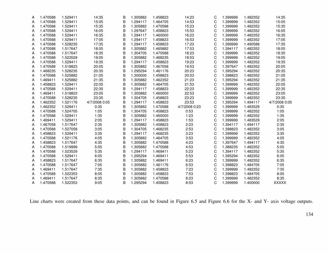
134

A 1.470588 1.529411 14:35 B 1.305882 1.458823 14:23 C 1.399999 1.482352 14:35 A 1.470588 1.529411 15:05 B 1.294117 1.464705 14:53 C 1.399999 1.482352 15:05 A 1.470588 1.529411 15:35 B 1.305882 1.470588 15:23 C 1.399999 1.482352 15:35 A 1.470588 1.529411 16:05 B 1.297647 1.458823 15:53 C 1.399999 1.482352 16:05 A 1.470588 1.529411 16:35 B 1.294117 1.460000 16:23 C 1.399999 1.482352 16:35 A 1.470588 1.529411 17:05 B 1.294117 1.458823 16:53 C 1.399999 1.482352 17:05 A 1.470588 1.528235 17:35 B 1.294117 1.458823 17:23 C 1.399999 1.490588 17:35 A 1.470588 1.517647 18:05 B 1.305882 1.465882 17:53 C 1.394117 1.482352 18:05 A 1.470588 1.517647 18:35 B 1.304705 1.470588 18:23 C 1.399999 1.482352 18:35 A 1.470588 1.523529 19:05 B 1.305882 1.468235 18:53 C 1.399999 1.482352 19:05 A 1.470588 1.529411 19:35 B 1.294117 1.458823 19:23 C 1.399999 1.482352 19:35 A 1.470588 1.518823 20:05 B 1.305882 1.467058 19:53 C 1.397647 1.482352 20:05 A 1.468235 1.528235 20:35 B 1.295294 1.461176 20:23 C 1.395294 1.482352 20:35 A 1.470588 1.525882 21:05 B 1.300000 1.458823 20:53 C 1.398823 1.482352 21:05 A 1.469411 1.525882 21:35 B 1.305882 1.462352 21:23 C 1.395294 1.482352 21:35 A 1.458823 1.529411 22:05 B 1.305882 1.464705 21:53 C 1.399999 1.482352 22:05 A 1.470588 1.529411 22:35 B 1.294117 1.458823 22:23 C 1.399999 1.482352 22:35 A 1.469411 1.518823 23:05 B 1.305882 1.460000 22:53 C 1.399999 1.482352 23:05 A 1.470588 1.528235 23:35 B 1.304705 1.458823 23:23 C 1.399999 1.482352 23:35 A 1.462352 1.521176 4/7/2008 0:05 B 1.294117 1.458823 23:53 C 1.395294 1.494117 4/7/2008 0:05 A 1.462352 1.529411 0:35 B 1.305882 1.470588 4/7/2008 0:23 C 1.399999 1.483529 0:35 A 1.470588 1.524705 1:05 B 1.304705 1.458823 0:53 C 1.399999 1.482352 1:05 A 1.470588 1.529411 1:35 B 1.305882 1.460000 1:23 C 1.399999 1.482352 1:35 A 1.469411 1.529411 2:05 B 1.294117 1.458823 1:53 C 1.399999 1.483529 2:05 A 1.467058 1.517647 2:35 B 1.305882 1.458823 2:23 C 1.394117 1.494117 2:35 A 1.470588 1.527058 3:05 B 1.304705 1.468235 2:53 C 1.398823 1.482352 3:05 A 1.458823 1.529411 3:35 B 1.294117 1.468235 3:23 C 1.399999 1.482352 3:35 A 1.470588 1.521176 4:05 B 1.305882 1.464705 3:53 C 1.399999 1.482352 4:05 A 1.458823 1.517647 4:35 B 1.305882 1.470588 4:23 C 1.397647 1.494117 4:35 A 1.470588 1.519999 5:05 B 1.305882 1.470588 4:53 C 1.388235 1.482352 5:05 A 1.470588 1.523529 5:35 B 1.294117 1.469411 5:23 C 1.394117 1.482352 5:35 A 1.470588 1.529411 6:05 B 1.295294 1.469411 5:53 C 1.395294 1.482352 6:05 A 1.458823 1.517647 6:35 B 1.305882 1.469411 6:23 C 1.399999 1.482352 6:35 A 1.470588 1.517647 7:05 B 1.305882 1.461176 6:53 C 1.398823 1.484705 7:05 A 1.469411 1.517647 7:35 B 1.305882 1.458823 7:23 C 1.399999 1.482352 7:35 A 1.470588 1.522353 8:05 B 1.305882 1.458823 7:53 C 1.398823 1.484705 8:05 A 1.469411 1.517647 8:35 B 1.305882 1.470588 8:23 C 1.399999 1.482352 8:35 A 1.470588 1.522353 9:05 B 1.295294 1.458823 8:53 C 1.399999 1.400000 XXXXX

Line charts were created from these data points, and can be found in Figure 6.5 and Figure 6.6 for the X- and Y- axis voltage outputs.

135

WORKS CITED

Accsense. (2007, August 7). Retrieved August 10, 2007, from Accsense: wireless

monitoring: http://www.accsense.com/

Advanced Circuits. (2008, January 29). $33 Each Special Offer. Retrieved January 29,

2008, from Advanced Circuits: http://www.4pcb.com/index.php?load=content&page_id=130

Advanced Circuits. (2008, January 29). Free DRM Report. Retrieved January 29, 2008,

from FreeDFM: https://www.freedfm.com/!freedfmstep1.asp

Analog Devices. (2008, April 9). ADXL103. Retrieved April 9, 2008, from Products:

http://www.analog.com/en/prod/0,,764_800_ADXL103%2C00.html


http://www.analog.com/en/prod/0,,764_800_ADXL203%2C00.html


http://www.analog.com/en/prod/0%2C2877%2CADXL330%2C00.html

Bird, J. P. (2008, April 8). Retrieved April 8, 2008, from Virginia Tech Unmanned

Systems Laboratory: www.me.vt.edu/Unmanned

Bird, J. P. (2007, October 29 & 31). Eagle Software. (J. P. Bird, Performer) Virginia

Tech, Randolph Hall, Blacksburg, VA, USA.

Brady, B. H., & Brown, E. T. (1985). Rock Mechanics For Underground Mining. New

York: Chapman & Hall.

Crossbow. (2007, August 10). Retrieved August 10, 2007, from Crossbow: Wireless

Sensor Networks: http://www.xbow.com/

CSMRS. (2006, May 16). Rock Mechanics. Retrieved June 5, 2007, from Central Soil

and Materials Research Station: http://www.csmrs.nic.in/rock.htm

136

Custom Computer Services, Inc. (2008, March 17). C Compilers. Retrieved March 17,

2008, from CCS Inc.: http://www.ccsinfo.com/content.php?page=compilers

Digi International. (2008, January 29). ZigBee/Mesh Modules. Retrieved January 29,

2008, from Digi International: http://www.digi.com/products/wireless/zigbee-mesh/xbee-series2-

module.jsp

Digi-Key. (2008, January 18). Retrieved January 29, 2008, from Digi-Key:

http://www.digikey.com/

Dubendorf, V. A. (2003). Wireless Data Technologies. John Wiley & Sons, Ltd.

E&MJ, & Anonymous. (June 2007). Stabilizing Influence. Engineering and Mining

Journal (E&MJ) , 60-63.

Eagle Electronics, Inc. (2005, March 17). Retrieved January 29, 2008, from Eagle

Electronics: http://www.eagle-elec.com/

Girard, J. M. (2006, April 17). Assessing and Monitoring Open Pit Mine Highwalls.

Retrieved June 15, 2007, from NIOSH: Mining:

http://www.cdc.gov/niosh/mining/pubs/pdfs/aamop.pdf

Girard, J. M., Mayerle, R. T., & McHugh, E. L. (2006, April 17). Advances in Remote

Sensing Techniques for Monitoring Rock Falls and Slope Failures. Retrieved June 4, 2007, from

NIOSH: http://www.cdc.gov/niosh/mining/pubs/pdfs/arst.pdf

Hartman, H. H., & Mutmansky, J. M. (2002). Introductory Mining Engineering (2nd ed.).

Hoboken: John Wiley and Sons, Inc.

Hoek, E., & Bray, J. W. (1981). Rock Slope Engineering: Revised Third Edition. London:

The Institution of Mining and Metallurgy.

137

Iannacchione, A. T., & Bajpayee, T. S. (2006, April 17). Forecasting Roof Falls with

Monitoring Technologies - A Look at the Moonee Colliery Experience. Retrieved June 12, 2007,

from NIOSH: Mining Safety: http://www.cdc.gov/niosh/mining/pubs/pdfs/frfwm.pdf

Iannacchione, A. T., Batchler, T., & Marshall, T. E. (2006, January 30). Mapping

Hazards with Microseismic Technology to Anticipate Roof Falls - A Case Study. Retrieved June

11, 2007, from NIOSH: Pittsburgh Research Laboratory:

http://www.cdc.gov/niosh/mining/pubs/pdfs/mhwmt.pdf

Larocque, G. (1977). Pit Slope Manual Chapter 8 - Monitoring (CANMET REPORT 77-

15 ed.). Ottawa, Canada: CANMET (Canada Centre for Mineral and Energy Technology,

formerly Mines Branch, Energy, Mines and Resources Canada).

Luxbacher, K. D. (2007). Time-Lapse Tomography of A Longwall Panel: A Comparison

of Location Schemes. 26th International Conference on Ground Control in Miing (pp. 217-224).

Morgantown, WV: West Virginia University.

Marshall, T. E., Prosser, L. J., & Iannacchione, A. T. (2006, January 30). Roof

Monitoring in Limestone-Experience with the Roof Monitoring Safety System (RMSS). Retrieved

June 11, 2007, from NIOSH: Mining: http://www.cdc.gov/niosh/mining/pubs/pdfs/rmile.pdf

McHugh, E. L., & Girard, J. M. (2006, April 17). Evaluating Techniques For Monitoring

Rock Falls and Slope Stability. Retrieved June 1, 2007, from NIOSH:

http://www.cdc.gov/niosh/mining/pubs/pdfs/etfmr.pdf

MEMSIC. (2008, January 14). MXR6999G/M Product Datasheet. Retrieved February 25,

2008, from MEMSIC: http://www.memsic.com/memsic/

MEMSIC. (2008, January 14). Products. Retrieved January 29, 2008, from MEMSIC:

solutions that make sense: http://www.memsic.com/memsic/

Microchip. (2008, January 29). Online Samples. Retrieved January 29, 2008, from

Microchip: http://sample.microchip.com/Default.aspx?testCookies=true

138

Microchip. (2004, December 23). Pin Diagrams. Retrieved April 8, 2008, from

PIC18F8722 Family Data Sheet: http://ww1.microchip.com/downloads/en/devicedoc/39646b.pdf

MicroStrain. (2007, August 10). Retrieved August 10, 2007, from MicroStrain:

Microminiature Sensors: http://www.microstrain.com/

Mill-Max. (2008, January 29). Order Free Samples. Retrieved January 29, 2008, from

Mill-Max Mfg. Corp.: http://www.mill-max.com/forms/sample_request.cfm

MSHA. (2008, March 14). MSHA Fatality Statistics. Retrieved April 14, 2008, from

Mine Safety and Health Administration: http://www.msha.gov/stats/charts/chartshome.htm

MSHA. (2007, July 19). Statistics Single Source Page. Retrieved July 24, 2007, from

Mine Safety and Health Administration: http://www.msha.gov/stats/Statistics.HTM

NIOSH. (2007, June 1). Ground Control Highlights. Retrieved June 1, 2007, from

NIOSH Mining Safety and Health Research:

http://www.cdc.gov/niosh/mining/highlights/programareahighlights1.htm

NIOSH. (2007, June 1). Slope Stability. Retrieved June 1, 2007, from NIOSH Mining

Safety and Health Topic: http://www.cdc.gov/niosh/mining/topics/topicpage15.htm

Pelican Cases. (2008, March 26). 1010 Micro Case. Retrieved March 26, 2008, from

Pelican: Global Headquarters: http://www.pelican.com/cases_detail.php?Case=1010

Phillip's Plastic and Machining LTD. (2008, February 06). Home. Retrieved March 28,

2008, from Phillip's Plastic and Machining LTD: http://philipsplastics.com/index.html

Prosser, L. J., Marshall, T. E., Tadolini, S. C., & Iannacchione, A. T. (2006, April 17).

Considerations for Using Roof Monitors in Underground Limestone Mines in the USA. Retrieved

June 11, 2007, from NIOSH: Pittsburgh Research Laboratory:

http://www.cdc.gov/niosh/mining/pubs/pdfs/cfurm.pdf

139

Sjöberg, J. (1996). Large Scale Slope Stability in Open Pit Mining - A Review. Sweden:

Division of Rock Mechanics, Luleå University of Technology.

Texas Instruments. (2008, January 29). Samples. Retrieved January 29, 2008, from Texas

Instruments: https://www-

a.ti.com/apps/samp/basket.asp?DCMP=TIHomeTracking&HQS=Other+OT+home_b_samples

The Weather Channel. (2008, April 8). Monthly Weather. Retrieved April 8, 2008, from

The Weather Channel: Local Weather: http://www.weather.com/

analysis of wireless tiltmeters for ground ... - virginia tech

Documents