analytical proof of newton's force lawssmile/guests/newton98b3.pdf · page 2 analytical proof...

Analytical Proof of Newton’s Force Laws

Analytical Proof of Newton's Force Laws1 Introduction

Many students intuitively assume that Newton's inertial and gravitational force laws, F ma= and

( )F G Mm

distance M m=

− 2 , are true since they are clear and

simple. However, there is an analysis that ties the two equations together and demonstrates that they must be true. The analysis provides answers to questions such as, "Is the inertial mass exactly the same as the gravitational mass? Why is the exponent of distance, 2, and not 1.99 or 2.01 or 1? Why is a constant required in one law and not in the other?"

The ideal way to prove new theoretical laws is to forecast the outcome of an experiment using the laws, perform the experiment, and find that the result is as forecast. But nature had already performed the experiment with planets in the solar system, and Kepler had determined the results. So, Newton, in his 1669 paper, "Mathematical Principles of Philosophy", (now part of the Great Books Series in local libraries), applied his force laws to the solar system and obtained the same results that Kepler had stated. This confirmed Newton's ideas, put physics on a firm mathematical basis and answered the above questions.

2 Summary of Analytical Proof of Newton's Force LawsIn the 8 step procedure that follows, Newton's force laws

are applied to the planet−sun system, and the planet (earth) path around the sun is shown to be an ellipse. This procedure below uses the mathematics found in first year college texts and explains the mathematics within the derivations as they are being evolved.

1. Observations show that the planets follow a smooth curve around the sun. Sketch the planet at position P, using polar coordinates, r and θ , within an orthogonal coordinate system.


2. Differentiate planet position functions to obtain planet velocities, v vx y and .

3. Differentiate planet velocities to obtain planet accelerations, a ax y and .

4. Equate Newton's inertial and gravitational force laws as applied to the planet. In this step we assume that inertial mass is identical to gravitational mass and that the force of gravity decreases as the square of distance. The acceleration required in the inertial law is also assumed to be the planet radial acceleration. G must also be assumed to make the equations consistent. The end result of this analytical procedure must show that all these assumptions are correct, or Newton’s equations would not be true.

5. Convert accelerations, a ax y and , to assumed planet radial, aR , and transverse, aT , accelerations.

6. Replace the time dependent term, ddt

θ, in the expression

of aR , with a function of r.

7. Replace the time dependent term, d rdt

2

2 , in the expression

of aR , with a function of r and θ.

8. Solve the differential equation containing r as a function of θ. The solution is the polar equation of an ellipse. This result is the same as Kepler's determination from astronomical data and analytically proves Newton's force equations.

2.1 Planet Position in Polar Coordinates, r and θThis analytical proof of Newton's force laws begins with a

planet P, moving along a smooth curve in a polar coordinate system as shown in Figure 1. The planet is moving relative to the stationary sun.


•

θ

Pr

x

y

0

yposition of P

x position of P

Figure 1

Sun

Earth

Radius vector, r, is attached to planet, P, and varies in length as P moves. Also, angle θ and its rate of change vary as P moves. Therefore, the velocity and acceleration of P vary continuously as the planet moves along its path. Recall that acceleration, velocity and force have magnitude and direction.

Newton had previously proved that, as far as the force of gravity was concerned, the entire mass of the planet and sun can be considered to be at the center of their spheres. The radius vector starts at the center of the sun and ends at the center of the planet.

Determine the x and y positions of P, as a function of r and θ, by using the trigonometric functions that are indicated by Figure 1.

The x distance of P from the origin; Px = r cos θ.The y distance of P from the origin; Py = r sin θ.

As time passes, P moves along its curve, making r and θ dependent upon time, t. The positions of P as functions of time are indicated as;

( ) ( ) ( )P t r t tx = cos θ ,( ) ( ) ( )P t r ty = sin tθ .

This completes step 1.


2.2 Planet Velocity in x and y Directions

Figure 2 indicates that the change in x and y distances is a function of both r and θ as P moves in time along its path.

•

θ

Pr

x

y

0

x velocity of P yposition of P

y velocity of P

x position of P

Figure 2

The velocity of the planet, P, is the change of distance along the curve per the change in time. Or,

change in distancechange in time

.st

= ∆∆

The calculus expression for velocity in the x direction, as

the change in time is made very small is; ( )ddt

Px t .

Velocity in the y direction is; ( ) ddt

P ty .


Therefore, the velocity of P in the x direction is;

( ) ( )( )v ddt

r t tx = cosθ .

And the velocity of P in the y direction is;

( ) ( )( )v ddt

r ty = sin tθ .

The calculus rule for obtaining the derivative of the product of two variables is to multiply the first term times the derivative of the second term plus the second times the derivative of the first.

Also, the derivative of the sine of an angle is the cosine of the angle times its derivative, and the derivative of the cosine of an angle is minus the sine of the angle times its derivative.

Using these differentiation rules;

The expression for the velocity of P in the x direction is,

( ) . dtdsin r

dtdrcoscos r

dtdv x

θθ−θ=θ=

The expression for the velocity of P in the y direction, following the same rules, is:

( ) . dtdcos r

dtdrsinsin r

dtdv y

θθ+θ=θ=



2.3 Planet Acceleration in x and y DirectionsThe next step is to obtain expressions for the planet

accelerations in the x and y directions indicated in Figure 3.

Acceleration in y direction

P•Acceleration in x direction

0

Figure 3

x

y

r

θ

Recall that acceleration is the rate of change of velocity.

Let the acceleration of the planet in the x direction be ax.

Let the acceleration of the planet in the y direction be ay.

Then; a ddt

vx x = ,

and addt

vy y = .

Finding acceleration causes us to take the derivative, with respect to time, of velocity. Velocity, in turn, is the derivative of distance with respect to time. Therefore, acceleration is the second derivative of distance with respect to time. The derivative of a derivative is called the second derivative. The symbol for the

second derivative, in this case is; ( )d r

dt

2

2variable or

.θ


Replace vx and vy with their derived expressions listed in Section 2.2. Follow the same differentiation rules as given above and obtain:

a d rdt

r ddt

r ddt

drdt

ddtx = −

− +

cos sin .θ θ θ θ θ2

2

2 2

2 2

a d rdt

r ddt

r ddt

drdt

ddty = −

+ +

sin sin .θ θ θ θ θ2

2

2 2

2 2


Accelerations ax and ay must be used to obtain expressions for the radial and transverse accelerations of the planet in Step 5.

2.4 Equate Gravitational Force to Planet Inertial Force Newton's force of gravity law as applied to earth mass, m,

and sun mass, M, is;

F GMmGravitational =

r 2 .

Where r is the radius vector, the varying distance from earth to sun, and G is the gravitational constant.

FGravitational is the amount of force that acts in a straight line between the planet and sun. This force would place the planet in free fall toward the sun if it were not for the counteracting planet inertial force.

What is the inertial force on the planet?

Newton’s inertial force law states that the inertial force is equal to the acceleration of the planet times the mass of the planet.

F mInertial Radial= a .


The inertial and gravitational forces must be equal to each other in magnitude but opposite in direction, or else the planet would leave its orbit. With unequal forces, the planet would fall into the sun, or attain a different orbit in a new equilibrium path, or go spinning off into space. Since the planet does maintain its orbit, the sum of the two forces must be zero.

F FGravitational Inertial+ = 0.

GMm m Radialra2 0+ = .

Divide through by m and obtain;GM

Radialra2 0+ = .

Then; GMr

aRadial2 = − .

This is an important place in the proof where the inertial mass is assumed to be identical to gravity mass and the radial acceleration is shown opposite to the attraction of gravity. We must continue to be skeptical of these assumptions, including distance to the second power, until we derive the elliptical path of the planet around the sun. This equation of the radial acceleration shows that aRadial is proportional to the inverse of distance squared. By applying some mathematics we will modify the equation to obtain aRadial as a function of r and θ. This radial acceleration equation is the basic equation that will evolve into the equation showing that the earth orbit is an ellipse.


Notice also that Newton's inertial force law can be considered simply as the definition of the unit of force. Once the standards of kilogram, meter and second are agreed upon, the unit of inertial force is established. We need a constant, (G), to make the gravitational units of force have the same dimensions and the same magnitude as inertial force units. But we have no reason (as yet), to believe that the inertial force, based on random but agreed upon standards, is directly proportional to the gravitational force. We just assumed the equivalence when we canceled "m" in the above derivation. If the path of the earth around the sun is analytically determined to be an ellipse, then the assumption is correct.


The next part of this proof to find expressions for radial and transverse planet accelerations in step 5 of the procedure.


2.5 Planet Radial and Transverse AccelerationsFigure 4 shows the geometric construction to determine

the radial and transverse planet accelerations.

axsinθ

aycosθ

aysinθ

axcosθ

θ

θ

θ

P

r

ax

ay

“a”aT

aR

x

y

0

Figure 4

A vector representing an assumed total planet acceleration, ”a”, is drawn at some angle to the radius vector, r. In Figure 4, it is convenient to draw “a” upward and away from the direction of the radial acceleration, aR, (which is opposite to the line of attraction between earth and sun).


One component of assumed planet acceleration, ”a”, must be in line with (but in the opposite direction to) the force of gravity between the sun and planet. This acceleration component, aR, is the radial acceleration . The other component of assumed planet acceleration, ”a”, placed perpendicular to the radial acceleration, is the transverse acceleration, aT. (This transverse acceleration, is not to be confused with the tangential, i.e. tangent to the path, acceleration. Tangential acceleration, not relevant in this proof, is discussed in Sections 7.1 and 7.2)

Of course, we know that if the planet actually has a transverse acceleration, a transverse force must be applied. But if a transverse force is applied, the planet will be pushed out of its orbit. So the transverse force must be zero and the transverse acceleration must also be zero. This concept of an assumed transverse acceleration, will provide one equation needed for this proof.

If the assumed acceleration, “a”, had been placed in line with the radius vector, it would have been identical to aR and no new information could be gained from the geometry. Placed as it is though, acceleration “a” is composed of two vectors, aR and aT. The radial acceleration, aR is drawn in line with the radius vector, r. The transverse acceleration, aT, is drawn perpendicular to the radial acceleration.

It is seen in Figure 4 that acceleration “a” is equal to two different sets of component vectors that provide the information needed to continue the proof. One set of these components is ax

and ay.

The second set of “a” components is aR and aT. The geometric construction in Figure 4 shows how aX, ay and θ are used to determine aR and aT.


The construction shows that;

a a aR x y= +cos sin .θ θ

a a aT y x= −cos sin .θ θ

The algebraic expressions for aX and aY were derived in Section 2.3.

Therefore, replace aX in aR and aT with

cos sin .θ θ θ θ θd rdt

r ddt

r ddt

drdt

ddt

2

2

2 2

2 2−

− +

Also, replace aY in aR and aT with

sin cos .θ θ θd rdt

r ddt

r d rdt

drdt

ddt

2

2

2 2

2 2−

+ +

Make the substitutions and obtain;

a d rdt

r ddtR = −

2

2

2θ .

a r d rdt

drdt

ddtT = +

2

2 2 θ .



2.6 Replace Time Dependent Term, ,ddt

θ in aR

From Section 2.4, GM

Radialra2 = − .

Replacing aRadial with its equivalent from above;

GMr

d rdt

r ddt2

2

2

2

= − −

θ .

A term that is not a function of time must be developed to

replace ddt

θ , because ddt

θ is a factor in aR.

Recall that we have already determined that aT is zero.

From above; a r d rdt

drdt

ddtT = +

2

2 2 θ .

Let’s take the derivative of r ddt

2 θ and see what results.

ddt

r ddt

r ddt

r drdt

ddt

2 22

2 2θ θ θ

= + .

Now multiply both sides by 1r

and obtain;

1 222

2rddt

r ddt

r ddt

drd

ddt

θ θθ

θ

= + ,which is aT.


But aT is zero. So, 1 2

rddt

r ddt

θ

is also zero.

Since 1r

cannot be zero, the derivative of r ddt

2 θ must be

zero. The rate of change of a constant is zero. Therefore, r ddt

2 θ

must be a constant. That constant is designated K.

Let K = r ddt

2 θ , andKr

ddt2 = θ .

Substitute K forr

ddt2

θ in the equation of radial acceleration,

− = −

G Mr

d rdt

r ddt2

2

2

2θ .

Then, − = −

G M Kr

d rdt

rr2

2

2 2

2

. 0r, − = −G M K 2

rd rdt r2

2

2 3.


Now d rdt

2

2 must be changed to a term containing r and θ,

and be time independent.


2.7 Replace Time Dependent Term, d rdt

2

2 , in aR

The factor to replace d rdt

2

2 is found through the following

procedure.

Let rn

= 1 . Differentiate 1n

with respect to time by

following the calculus rule for differentiating a variable to a power. The rule is: Place the exponent in front of the variable, subtract one from the exponent and differentiate the variable.

The result is,ddt n n

dndt

1 12

= − .

Then,drdt n

dndt

= − 12 .Multiply − 1

2ndndt

by 1 in the form of dd

θθ

.

drdt n

dnd

ddt

= − 12 θ

θ .

In Section 2.6, we found that ddt

θ is equal to Kr 2 .

Substitute and obtain; drdt n

dnd r

dnd

= − = −12 2θ θ

K K .

We want to replace the second derivative of r with respect

to t, therefore we must differentiate the first derivative, drdt

, once

more to obtain the second derivative.

This second derivative is, d r

dt

d n

d

ddt

2

2

2

2 = K−

θ

θ .


We again substitute Kr 2 for d

dtθ , and obtain;

d rdt

n d nd

2

22 2

2

2= − Kθ

.

The result from Step 6 above is − = −G M Kr

d rdt r2

2

2

2

3 .

Substituting for d rdt

2

2 we obtain;

− = − −GM K Kr

n d nd r2

2 22

2

2

3θ.

Since nr

= 1,

GM K Kr r

d nd r2

2

2

2

2

2

3= +θ

.

This is the point in the analytical proof where distance squared must be in the denominator of the gravitational force. In order for the analysis to conclude with a closed curve we must have distance, r, the radius vector, exactly to the first power. When we multiply through with r2,, we will have r to the first power within the equation. It will then be possible for the radius vector to trace a smooth curve as we assumed in Figures 1 to 4.The second derivative term will determine the shape of the curve.

GM K K= +22

2

2d nd rθ

.

This completes Step 7.


2.8 Obtain r as a Function of θ and Confirm Kepler's First Law

Simplify the above equation by replacing 1r

nwith .

d nd

n2

2 2 0θ

+ − =GMK

.

This is the differential equation to be solved in order to get r as a function of θ. We know, from Section 2.2 Step 2, that the derivative of a cosine function is a negative sine function and the derivative of the sine function is a cosine function. It appears that the cosine function of θ will fit into the differential equation and solve it. The procedure to solve the equation is to let,

n = +A GMK

cos ,θ 2 where A is another constant.

What is the first derivative of n with respect to θ ? dnd

ddθ θ

θ θ=

= −Acos + GMK

A2 sin .

What is the second derivative of n with respect to θ ?

d nd

2

2θθ= − A cos .

To test this solution, put n and the second derivative of n with respect to θ back into the original equation and check the result.

d nd

n2

2 2 0θ

GMK

+ − = .

− + + − =A A GMK

GMK

cos cos .θ θ 2 2 0

The left side of the test equation is also zero.The result shown in Step 7 is:

GM K K= +22

2

2d nd rθ

.

Substitute − Acosθ for the second derivative of n with respect to θ.

( )GM K A K= − +22

cos .θr


Solve for r and obtain;

r =+

KGM

KGM

A

2

21 cos

.θ

The radius vector determining the earth’s path around the sun is a function of the mass of the sun, the cosine of the generated angle and constants G, K, and A. This is Newton's derived equation for the planet's path around the sun and it has the form of the polar equation of a conic. (See Section 3.) This analytically derived path turns out to be an ellipse and agrees with Kepler's first law. Notice again that the mass of the earth plays no part in its equation of motion. An object of a far different size and mass would occupy the same path if it had the same radial acceleration.

This same phenomenon occurs in Cavendish’s horizontal pendulum experiment to “Weigh the earth”. The mass of the small bob and the large attracting sphere both appear to be used in finding G. But on closer inspection we find that the mass of the bob is used in calculating its moment of inertia and again in the multiplication of the mass of the bob and the large attracting sphere for gravity force. So that the mass of the small bob cancels out. However, physics texts often show the mass of the small bob to be necessary for the calculation of G in the Cavindish experiment.

The above equation of motion of the earth’s radius vector was derived using only Newton's force laws and it was an extremely important result. It helped make Newton's laws the basis of mechanical physics.

This completes Step 8 and the analytical proof of Newton's force laws. The proofs of Kepler’s second and third laws are in Sections 4 and 5.


3 Polar Equation of Conics

Recall that one polar equation of a conic is; r =+

d cosε

ε θ1.

Where r is the radius vector, and d is the distance from focus to directrix. The radius vector generates the angle θ and traces out the conic. The planet orbit starts in Figure 1 and completes the ellipse in Figure 5.

b

a aε

aε

r=a

θr

a(1-ε )

Sun FocusFocus

Directrix

d

Figure 5

If the eccentricity, ε, is less than one and greater than zero, the plotted equation is an ellipse with the sun at a focus. (When ε equals one the equation is a parabola. When ε is greater than one the equation is an hyperbola.)

If the path of the planet is an ellipse, the planet will return to some starting point once every orbit. The earth returns to a randomly selected starting point, as do all the planets. So, using only his equations, Newton proved that the path of the earth is an ellipse as Kepler had observed. Therefore Newton's equations are proved to be correct. Since all the planets and their moons follow elliptical paths, they all demonstrate Newton’s laws.


To follow the proofs of Kepler’s laws, we need more information on the mathematical characteristics of an ellipse.

In Figure 5:

r = radius vector.

θ = angle generated by radius vector, 0o - 360o. When θ goes beyond 360o the curve repeats just as the planet repeats its orbit.

a = semi-major axis. This is also the "mean" planet-sun distance.

b = semi-minor axis.

ε = eccentricity.

ε of earth orbit =.017. ε of moon orbit = .06.

Area of ellipse = πab.

Polar equations of ellipse;

r r=+

=−

d and

a

1+

2

εε

ε

εθ θ1

1

cos cos.

The second equation shows that when the eccentricity, ε, is zero, the conic is a circle of radius a. Since the planet's observed distance to the sun varies, the planet path cannot be a circle and ε cannot be zero.


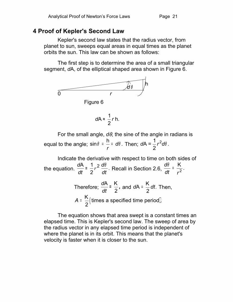
4 Proof of Kepler's Second LawKepler's second law states that the radius vector, from

planet to sun, sweeps equal areas in equal times as the planet orbits the sun. This law can be shown as follows:

The first step is to determine the area of a small triangular segment, dA, of the elliptical shaped area shown in Figure 6.

Figure 6

d θr

h

0

d rA 12

h.≈

For the small angle, dθ, the sine of the angle in radians is

equal to the angle; sin .θ θ= =hr

d Then; d r dA = 12

2 θ .

Indicate the derivative with respect to time on both sides of

the equation. ddt

ddt

A .= 12

2r θ Recall in Section 2.6,

ddt r

θ = K2 .

Therefore; ddtA K=

2, and d dtA K=

2. Then,

( )A = K2

times a specified time period .

The equation shows that area swept is a constant times an elapsed time. This is Kepler's second law. The sweep of area by the radius vector in any elapsed time period is independent of where the planet is in its orbit. This means that the planet's velocity is faster when it is closer to the sun.


5 Proof of Kepler's Third LawKepler's third law states that, the square of the planet's

time for one orbit, divided by the cube of the mean distance of planet to sun, is equal to the same constant for all planets.

From the proof of Kepler's second law (Section 4) we note

that; d dtA K=2

.

The planet sweeps through the whole area of the ellipse, π a b, in the time "T" that it takes to orbit the sun.

The total area swept by vector r in time T is,

π ab K T.=2

Then, TK ab= 2π .

Kepler's law requires T2. So, squaring each side,

TKa b

22 4 2 2 2

= π .

From Section 3 discussion of ellipse characteristics and Figure 5:

a b a2 2 2 2= + ε .

b a a a2 2 2 2= − = −

ε ε2 21 .

Then TK

2

4

2

a=

−4 2 21π ε

.


Next equate the numerators of the analytic equations of

the ellipse; 1 2− =ε εda

.

Then, Ta K

2

3 2d= 4 2π ε .

The equation of an ellipse in polar coordinates is,

r = d1+

εε θcos

.

And Newton's planetary orbit equation is,

r =

KGM

1+ KGM

Acos

2

2θ

.

So for planetary orbiting motion,d KGM

2ε = .

Then, Ta GM

2

3 = 4 2π .

Therefore, for every planet Ta

2

3 is equal to the same

constant. (Note that each planet has a different constant in Kepler's second law.)

Newton equations again proved an astronomically observed Kepler law, gave the mathematical principles involved and determined exactly the value of the constant .


6 Newton's Analytical Estimate of GThe following procedure is one of Newton’s estimate of G

based on his own force laws.

1. Inertial force, FI = m a.

2. At the Earth’s surface; inertial force FI= mass of any object times the acceleration due to earth's gravity. The acceleration due to earth's gravity, g, was found by Galileo to be 9.8 meters /sec2.Inertial force, FI, at earth's surface = mass of any object X g.

3. Gravitational force, F GM x m

RadiusGEarth Object

Earth2= .

4. The unit of inertial force is kg-meter per second2. To make the unit of gravitational force consistent, G has the dimension of kg-meter per second2 times meter2 over kg2.The unit of force, kg-meter per second2, is now named the “newton”.

5. FI = FG = mObject X 9.8 m/sec2 =GM x m

RadiusEarth Object

Earth2 .


The mass of the object is on both sides of the equal sign and cancels.

Then, 9 8. .= GMRadiusEarth

2

Newton estimated that the average density of the earth was between 5 and 6 times the density of water. Using 5.5 times the density of water, and an estimated radius and volume of earth, the value of G is determined to be; 7 X 10-11 m3 / kg sec2.

The present day value is 6.67 X 10-11 m3 / kg sec2.

This value of G enabled astronomers to estimate the mass of many bodies in the solar system and correlate the estimates with the measured distances of moons, planets and sun, and velocities of moons and planets. This also indicated that G is a universal constant.

7 Two Methods of Calculating Moon Radial AccelerationThere are two methods of calculating the radial

acceleration of the moon using Newton’s laws:

1. The first method requires calculating g times the ratio of the earth radius2 to moon's distance2. When we know the radial acceleration of the moon at its mean distance from earth we can calculate G MEarth, and modify the estimates of earth mass or G by using Newton's force laws.

2. The second method requires that astronomers provide the tangential velocity of the moon at its mean distance from the earth. The tangential velocity squared divided by the mean distance moon-earth also results in radial acceleration.


7.1 First Method of Calculating Moon Radial Acceleration.Recall that the weight of an object on the earth surface is

the mass of the object times the acceleration due to earth's gravity, g. By using g and Newton’s equations we can calculate the radial acceleration of the moon.

Astronomical data:

Mean distance (semi-major axis of ellipse; moon center to earth center) is 3.84 X 108 meters.

Moon's tangential velocity is 1.02 meters per second at its mean distance from earth.

Earth radius is 6.38X106 meters.

Acceleration due to earth's gravity, g, is 9.8 m/sec2.

First method procedure:

Gravitational force = GM x m

Radius= m xg.Earth Object

EarthObject

2

g is the acceleration experienced by the object on the earth's surface pointing to the earth center.

gGM

RadiusEarth

Earth2

= .


The moon is staying in its orbit around the earth for the same reason that the earth stays in its orbit around the sun. The radial acceleration of the moon is exactly equal and opposite the acceleration caused by earth-moon gravity attraction on the moon. Equate moon inertial force to gravitationalforce.

m a = Gm M

Distancemoon

EarthRadial moon

moon

Earth -moon2

− .Cancel the moon

mass from both sides of the equation. Here again we cancel out the small (moon) mass just as the earth mass was cancelled in developing Newton’s equation of earth motion.The cancelling of the small bob mass in the Cavendish gravity experment follows the same

reasoning. a GM

DistanceRadial moon

Earth

Earth-moon2

= − .

From above; 9 8. .= − GM

RadiusEarth

Earth2

Since the ratio of these two equations is

another equality,a

GM

DistanceGM

Radius

Radial moon

Earth

Earth-moon2

Earth

Earth2

9 8.,=

−

The radial acceleration of the moon can now be determined.

a Radius

Distance m / secRadial moon

Earth2

Earth-moon2

2= − = −9 8 0027. . .

It is only at this point in space, when the moon is at its mean distance from earth, that the moon has exactly this radial acceleration. When the moon is closer to earth in its elliptical orbit, the magnitude of the radial acceleration is greater. When the moon is further from earth, the magnitude of radial acceleration is less.


7.2 Second Method of Calculating Moon Radial AccelerationThe second method used for calculating the radial

acceleration of the moon, requires dividing the square of the moon tangential velocity, at its mean distance from earth, by that distance. (The semi-major axis of an ellipse is its mean distance, designated by the letter, ”a”.)

As an equation; V

Mean Distancem / secTangential

2

Earth-moon

2= . .0027

This result confirmed Newton's ratio method of calculating the radial acceleration of the moon.

How do we prove analytically that, V

Mean DistanceaTangential

2

Earth-moonRradial moon= ?

An approximation of radial acceleration can be made by assuming that the orbit of the moon around the earth is a circle. But Newton has shown that the path is an ellipse. The assumption is then wrong for four reasons:

1. The moon's orbit is an ellipse.

2. The tangential velocity is not constant.

3. The radial acceleration is not constant.

4. The radial acceleration of the moon is in line with the focus of an ellipse (the center of the earth), and not at the center of a circular path. Using moon's velocity squared divided by an assumed radius gives an assumed centripetal acceleration.

Therefore we must find the radial acceleration of the moon, as a function of tangential velocity and the ellipse radius vector, to show that both methods of calculating the moon's radial acceleration are correct.


7.2.1 Conservation of Orbital EnergyIn order to obtain an equation of radial acceleration as a

function of tangential velocity, we have to consider the conservation of orbital, i.e. mechanical, energy of the moon as it orbits the earth. We will combine the orbital energy equation with Newton's planet ellipse equations in order to obtain an equation for the moon's tangential velocity. Then we can equate this tangential velocity to Newton's equation and obtain the moon's radial acceleration.

The conservation of energy concept, as applied to the moon, means that the total mechanical energy of the moon must be constant for the moon to maintain its elliptical orbit.

The total orbital energy of the moon is the algebraic sum of its kinetic energy, K E, and its potential energy, P E. There is an exchange of small percentages of P E and K E as the moon orbits the earth.


7.2.1a Development of First Orbital Energy EquationThe P E of the moon is considered to be zero at an infinite

distance from the earth. When the infinite distance from the earth is selected as the reference level, the P E of the mass of the moon, m at a distance r, from the earth, M, is:

P E G M m= −r

.

This equation shows that the increase in the moon's P E, when its mass was brought to the orbital position, is equal to the negative of the work done by the earth's gravity field.

The K E of the moon is equal to 12

mv2 , where v is the

tangential or orbital velocity that varies during the elliptical orbit.

E (total mechanical or orbital energy) = K E + P E.

E 12

mv G M mOrbital

2= −r

.

The equation shows that when the moon approaches its perigee and gets closer to earth, the P E changes to a larger negative value but the K E grows larger as the moon's velocity is increasing, and the orbital energy remains constant.

The above orbital energy equation is the first equation, of the two that are needed, for this calculation method. It shows orbital energy as a function of the ellipse radius vector and tangential velocity. G, M, and m are constant. The second equation will give the orbital energy at a certain point in the orbit, (at perigee). But since orbital energy is constant, the designated orbital energies can be equated.


7.2.1b Development of Second Orbital Energy EquationWe will now obtain the second equation of EOrbital. These

two equations will enable us to finally show the connection between tangential velocity and radial acceleration.

As derived below, the differential calculus equation for the variable tangential velocity of an object moving some distance along any smooth curve (such as an ellipse) is:

VTangential2 =

+

drdt

r ddt

22

2θ .

This equation is developed by considering a small increase in angle θ and distance r, with a small increase in time, indicated in Figure 7.

θ

r

r

∆ r

h ∆ s

s distance

Figure 7

rdθ

0

For small angles, where sin θ equals θ, h = r dθ.

( ) ( ) ( )∆ ∆ ∆s 2 2 2= +r r θ .

Designate a change of, s, r and θ due to a ∆ increase in time:

∆∆

∆∆

∆∆

st

=

+

2 2 2rt

rtθ .


As the change in time is made smaller and approaches zero , we obtain the calculus expression for the tangential velocity along the curve.

VTangential2 =

+

drdt

r ddt

22

2θ .

The change in swept angle with respect to time, is the same function of r found in section 2.6 ;

ddt r

θ

= k2 .

This equation applies to the planet-moon systems (with the different constant because the elliptical path is different) as well as to the sun-planet system.

Substituting; V kTangential2

2=

+

dr

dt r

2

2 .

As seen in Figure 6, there are several things to note concerning the moon’s elliptical path at perigee.

r=aperigee

rmina-aε

a

•Earthcenter

Focusθ

Tangentialvelocity, V

Figure 6

aε

Moon•


The moon's radius vector goes through a minimum length at perigee. The radius vector length at perigee is, a(1-ε).

At the perigee the rate of change of the radius vector length is zero.

For the ellipse, with θ being generated by the radius vector starting at the perigee, the derivative of r with respect to time is 0, when θ =00.

Therefore, drdt

is zero and can be removed from the

standard equation for the object tangential velocity on an ellipse at perigee.

The tangential velocity equation reduces to;

V kTangential2

2

Perigee

=r 2 .

The polar equation for the moon's elliptical orbit is the same form as the one that Newton determined for earth.

r =+

kGMk

GMBcos

2

Earth2

Earth1 θ

.

From Section 3, a general equation for an ellipse is:

r =

a 1-

1+ cos

ε

ε θ

2

."a" is the semi-major axis of the ellipse and

is called the mean distance of an ellipse.


Equating the numerators of the equivalent ellipse equations:

kGM

a 1-2

Earth=

ε 2 .

From Figure 6, r at perigee = a(1-ε).

The next step is to calculate the moon's energy at perigee.

Energy at perigee = K E - P E.

Since V = kTangential2

2

Perigee2r

,

E m k GMmPerigee

2

Perigee2

Perigee= −1

2 r r.

From above;

k GM a 1-2 2=

ε .

Substituting for k2 in the energy at perigee equation and simplifying;

E GMm2a

EPerigee Orbital= − = .

The orbital energy of the moon at perigee is the same as the orbital energy at any other place in its orbit.

This is the second equation of EOrbital that is needed to show the relationship between VTangential and radial acceleration.


7.3 Relation of Moon Tangential Velocity and Radial AccelerationWe will first obtain the moon's tangential velocity as a

function of its radius vector by equating the two energy equations.

First equation; E mV GMmOrbital Tangential= −1

22

r.

Second equation; E GMm2aOrbital = − .

Equate the orbital energy equations and solve for VTangential

2 .

V GM 2aTangential

2 = −

r

1 .

We will now find another expression for radial acceleration.

In Section 2.4, we found that the general expression for the radial acceleration of earth orbiting the sun (or moon orbiting the earth) is;

arRadial

GM= 2 .Wherein, M is the mass of the sun.

In the earth-moon system, M is the mass of the earth.

arRadialEarthGM= 2 .

When r = mean distance, a,

aRadialEarth2

GMa

= .


We just found that, V GMaTangential

2 Earth= .

Dividing both sides by mean distance “a” results in;

Va

GMa

Tangential2

earth2= .

This is the radial acceleration of the moon at the mean distance, “a”, from the earth as proven in Section 7.1.

We have just shown why Va

2 can be used for the

radial acceleration of the moon and the equation looks like the equation for the centripetal acceleration of an object revolving in a circle. But we must always use VTangential at the mean (semi-major axis) distance of moon to earth (or earth to sun) and, of course, use the semi-major axis for the distance. And this radial acceleration is true at only two places (or times) on each orbit.

As shown above , we have evolved two more equations of planetary (or moon ) motion:

One: The radial acceleration of a planet (or moon) is V

aTangential2

at the mean distance, a, from the sun (or planet).

Two: V GM 2aTangential

2 = −

r

1is applicable to observations

of all the planets (or moons) and enables accurate cross-checking of observed distances and tangential velocities.


8 Conclusions Shown by this Analysis of Newton’s LawsThe conclusion to be drawn here is that each one of

Newton's laws is proven by his analysis of planetary motion. He confirmed exactly the empirical data of Kepler, and in addition, he has shown mathematically why the data is true. If any part of Newton's work was incorrect, he could not have arrived at the equation of planet elliptical motion about the sun.

When equating force of gravity and inertial force, we found that the mass of the earth canceled out. This means that inertial mass and gravity mass are exactly the same. Also, any size object in the earth's orbit will orbit the sun exactly as earth if it has the same radial acceleration as earth.

Newton proved conclusively that the orbital path of a planet (or moon) is an ellipse with the sun (or planet) at a focus. This is a remarkable fact in itself. But more remarkable is that Newton proved his own laws at the same time, and introduced calculus into his work. He proved that all the planets, and the moons or satellites orbiting the planets (and comets) follow his laws.

Newton proved F = ma,

( )the force of gravity G

m m

Distance m to m 1 2

22

1

= ,and action

equals reaction, in that the planet attracts the sun with the same force that the sun attracts the planet. Newton proved that the force of gravity decreases exactly as 1/r2.

Newton estimated G by using his own laws, and showed that G is a universal constant.

Newton's laws are always in use in problem solving. They form the basis of mechanical physics and engineering, momentum, work, satellite positioning, moon landings and calculations involving binary stars.

analytical proof of newton's force lawssmile/guests/newton98b3.pdf · page 2 analytical proof...

Documents