analyzing market-based resource allocation strategies for
TRANSCRIPT

Analyzing Market-based Resource Allocation Strategies for theComputational Grid ∗
Rich Wolski† James S. Plank† John Brevik‡ Todd Bryan†
† Department of Computer ScienceUniversity of Tennessee
‡ Mathematics and Computer Science DepartmentCollege of the Holy Cross
Abstract
In this paper, we investigate G-commerce —computational economies for controlling resourceallocation in Computational Grid settings. We de-fine hypothetical resource consumers (represent-ing users and Grid-aware applications) and re-source producers (representing resource ownerswho “sell” their resources to the Grid). We thenmeasure the efficiency of resource allocation un-der two different market conditions: commoditiesmarkets and auctions. We compare both mar-ket strategies in terms of price stability, marketequilibrium, consumer efficiency, and producerefficiency. Our results indicate that commoditiesmarkets are a better choice for controlling Gridresources than previously defined auction strate-gies.
1 Introduction
With the proliferation of the Internet comes thepossibility of aggregating vast collections of com-
∗This work was supported in part by NSF grants EIA-9975020, EIA-9975015, and ACI-9876895.
puters into large-scale computational platforms.A new computing paradigm known as the Com-putational Grid [17, 3] articulates a vision of dis-tributed computing in which applications “plug”into a “power grid” of computational resourceswhen they execute, dynamically drawing whatthey need from the global supply. While a greatdeal of research concerning the software mecha-nisms that will be necessary to bring Computa-tional Grids to fruition is underway [3, 16, 20, 8,4, 24, 21, 1, 34], little work has focused on theresource control policies that are likely to suc-ceed. In particular, almost all Grid resource al-location and scheduling research espouses one oftwo paradigms: centralized omnipotent resourcecontrol [18, 20, 28, 29] or localized applicationcontrol [9, 4, 2, 19]. The first is certainly not ascalable solution and the second can lead to un-stable resource assignments as “Grid-aware” ap-plications adapt to compete for resources.
In this paper, we investigateG-commerce—the problem of dynamic resource allocation on theGrid in terms of computationalmarket economiesin which applications must buy the resources theyuse from resource suppliers using an agreed-uponcurrency. Framing the resource allocation prob-

lem in economic terms is attractive for severalreasons. First, resource usage is not free. Whileburgeoning Grid systems are willing to make re-sources readily available to early developers asa way of cultivating a user community, resourcecost eventually must be considered if the Grid isto become pervasive. Second, the dynamics ofGrid performance response are, as of yet, diffi-cult to model. Application schedulers can makeresource acquisition decisions at machine speedsin response to the perceived effects of contention.As resource load fluctuates, applications can ad-just their resource usage, forming a feedback con-trol loop with a potentially non-linear response.By formulating Grid resource usage in marketterms, we are able to draw upon a large body ofanalytical research from the field of economicsand apply it to the understanding of emergentGrid behavior. Last, if resource owners are to beconvinced to federate their resources to the Grid,they must be able to account for the relative costsand benefits of doing so. Any market formulationcarries with it an inherent notion of relative worthwhich can be used to quantify the cost-to-benefitratio for both Grid users and stake-holders.
While there are a number of different plausibleG-commerce market formulations for the Grid,we focus on two broad categories:commodi-ties markets andauctions. The overall goal ofthe Computational Grid is to allow applicationsto treat computational, network, and storage re-sources as individual and interchangeable com-modities, and not specific machines, networks,and disk or tape systems. Modeling the Grid as acommodities market is thus a natural choice. Onthe other hand, auctions require little in the wayof global price information, and they are easy toimplement in a distributed setting. Both types ofeconomies have been studied as strategies for dis-tributed resource brokering [11, 35, 25, 6, 7, 10].Our goal is to enhance our deeper understandingof how these economies will fare as resource bro-kering mechanisms for Computational Grids.
To investigate Computational Grid settings and
G-commerce resource allocation strategies, weevaluate commodities markets and auctions withrespect to four criteria:
1. Grid-wide price stability
2. Market equilibrium
3. Application efficiency
4. Resource efficiency
Price stability is critical to ensure scheduling sta-bility. If the price fluctuates wildly, applicationand resource schedulers that base their decisionson the state of the economy will follow suit, lead-ing to poor performance, and therefore ineffec-tiveness of the Grid as a computational infrastruc-ture. Equilibrium measures the degree to whichprices are fair. If the overall market cannot bebrought into equilibrium, the relative expense orworth of a particular transaction cannot be trusted,and again the Grid is not doing its job. Applica-tion efficiency measures how effective the Gridis as a computational platform. Resource effi-ciency measures how well the Grid manages itsresources. Poor application and/or resource ef-ficiency will mean that the Grid is not succeed-ing as a computational infrastructure. Thus, weuse these four criteria to evaluate how well eachG-commerce economy works as the basis for re-source allocation in Computational Grids.
The remainder of this paper is organized as fol-lows. In the next section, we discuss the specificmarket formulations we use in this study. Sec-tion 3 describes the simulation methodology weuse and the results we obtain for different hypo-thetical market parameterizations. In Section 4we conclude and point to future work.
2 G-commerce — Market Economiesfor the Grid
In formulating a computational economy forthe Grid, we make two assumptions.#1: The rel-
2

ative worth of a resource is determined by its sup-ply and the demand for it.This assumption is im-portant because it rules out pricing schemes thatare based on arbitrarily decided priorities. For ex-ample, it is not possible in an economy for anorganization to simply declare what the price ofits resources are and then decree that its userspay that price even if cheaper, better alternativesare available. While there are several plausiblescenarios in which such Draconian policies areappropriate (e.g. users are funded to use a spe-cific machine as part of their individual researchprojects), from the perspective of the Grid, the re-source allocation problem under these conditionshas been solved.
Further, we assume that supply and demand arefunctions of price, and that true relative worth isrepresented at the price-point where supply equalsdemand – that is, at market equilibrium. Con-versely, at a non-equilibrium price-point (wheresupply does not equal demand), price either over-states or understates relative worth.
#2: Resource decisions based on self-interestare inescapable in any federated resource system.If we are to simulate a computational economy,we must ultimately hypothesize supply and de-mand functions for our simulated producers andconsumers respectively. Individual supply anddemand functions are difficult to measure at best,particularly since there are no existing Compu-tational Grid economies which we can observe.Our admittedly less-satisfactory approach is todefine supply and demand functions that representeach simulated producer and consumer’s “self-interest.” An individual consumer buys only ifthe purchase is a “good deal” for that consumer.Analogously, producers sell only when a sale is intheir best interest.
In the next section, we detail the specific func-tions we investigate, but generally our approachrelies on these two assumptions.
2.1 Producers and Consumers
To compare the efficacy of commodities mar-kets and auctions as Grid resource allocationschemes, we define a set of simulated Gridproducers and consumers representing resourceproviders and applications respectively. We thenuse the same set of producers and consumers tocompare commodity and auction-based marketsettings.
We simulate two different kinds of producersin this study: producers of CPUs and produc-ers of disk storage. That is, from the perspec-tive of a resource market, there are two kindsof resources within our simulated Grids: CPUsand disks. While the results should generalizeto include a variety other commodities, networkspresent a special problem. Our consumer modelis that an application may request a specifiedamount of CPU and disk (the units of which wediscuss below) and that these requests may be ser-viced by any provider regardless of location ornetwork connectivity. Since network links can-not be combined with other resources arbitrarily,they cannot be modeled as separate commodities.We believe that network cost can be representedin terms of “shipping” costs in more complicatedmarkets, but for the purposes of this study, weconsider network connectivity to be uniform.
2.1.1 CPU Producer Model
In this study, a CPU represents a computationalengine with a fixed dedicated speed. A CPU pro-ducer agrees to sell to the Grid some number offixed “shares” of the CPU it controls. The real-world scenario for this model is for CPU ownersto agree to host a fixed number of processes fromthe Grid in exchange for Grid currency. Each pro-cess gets a fixed, pre-determined fraction of thededicated CPU speed, but the owner determineshow many fractions or “slots” he or she is willingto sell. For example, in our study, the fraction is10% so each CPU producer agrees to sell a fixed
3

number (less than 10) of 10%-sized slots to theGrid. When a job occupies a CPU, it is guaran-teed to get 10% of the available cycles for eachslot it consumes. Each CPU, however, differs inthe total number of slots it is willing to sell.
To determine supply at a given price-point,each CPU calculates
mean price = revenue/now/slots (1)
whererevenue is the total amount of Grid cur-rency (hereafter referred to as $G which is pro-nounced “Grid bucks”),now is an incrementingclock, andslots is the total number of processslots the CPU owner is willing to support. Themean price value is the average $G per time unitper slot the CPU has made from selling to theGrid. In our study, CPU producers will only sellif the current price of a CPU slot exceeds themean price value, and when they sell, they sellall unoccupied slots. That is, the CPU will sell allof its available slots when it will turn a profit (perslot) with respect to the average profit over time.
2.1.2 Disk Producer Model
The model we use for a disk producer is similarto that for the CPU producer, except that diskssell some number of fixed-sized “files” that ap-plications may use for storage. Themean pricecalculation for disk files is
mean price = revenue/now/capacity (2)
wherecapacity is the total number of files a diskproducer is willing to sell to the Grid. If the cur-rent price for a file is greater than themean price,a disk producer will sell all of its available files.
Note that the resolution of CPU slots and filesizes is variable. It is possible to make a CPUslot equivalent to the duration of a single clockcycle, and a disk file be a single byte. Since ourmarkets transact business at the commodity level,however, we hypothesize that any real implemen-tation for the Grid will need to work with larger-
scale aggregations of resources for reasons of effi-ciency. For the simulations described in Section 3we choose values for these aggregations that webelieve reflect a market formulation that is cur-rently implementable.
2.1.3 Consumers and Jobs
Consumers express their needs to the market inthe form of jobs. Each job specifies both a sizeand an occupancy duration for each resource tobe consumed. Each consumer also sports a bud-get of $G that it can use to pay for the resourcesneeded by its jobs. Consumers are given an initialbudget and a periodic allowance, but they are notallowed to hold $G over from one period until thenext. This method of budget refresh is inspired bythe allocation policies currently in use at the NSFPartnerships for Advanced Computational Infras-tructure (PACIs). At these centers, allocations areperishable.
When a consumer wishes to purchase resourcesfor a job, it declares the size of the request foreach commodity, but not the duration. Our modelis that job durations are relatively long, and thatproducers allow consumers occupancy withoutknowing for how long the occupancy will last. Atthe time a producer agrees to sell to a consumer,a price is fixed that will be charged to the con-sumer for each simulated time unit until the jobcompletes.
For example, consider a consumer wishing tobuy a CPU slot for 100 minutes and a disk file for300 minutes to service a particular job. If the con-sumer wishes to buy each for a particular price, itdeclares to the market a demand of 1 CPU slotand 1 disk slot, but does not reveal the 100 and300 minute durations. A CPU producer wishingto sell at the CPU price agrees to accept the jobuntil the job completes (as does the disk producerfor the disk job). Once the sales are transacted, theconsumer’s budget is decremented by the agreed-upon price every simulated minute, and each pro-ducer’s revenue account is incremented by the
4

same amount. If the job completes, the CPU pro-ducer will have accrued 100 times the CPU price,the disk producer will have accrued 300 times thedisk price, and the consumer’s budget will havebeen decremented by the sum of 100 times theCPU price and 300 times the disk price.
In defining this method of conducting resourcetransactions, we make several assumptions. First,we assume that in an actual Grid setting resourceproducers or suppliers will commit some fractionof their resources to the Grid, and that fraction isslowly changing. Once committed, the fraction“belongs” to the Grid so producers are not con-cerned with occupancy. This assumption corre-sponds to the behavior of some batch systems inwhich, once a job is allowed to occupy its proces-sors, it is allowed to run either until completion,or until its user’s allocation is exhausted. Produc-ers are concerned, in our models, with profit andthey only sell if it is profitable on the average. Byincluding time in the supply functions, producersconsider past occupancy (in terms of profit) whendeciding to sell. We are also assuming that nei-ther consumers nor producers are malicious andthat both honor their commitments. In practice,this requirement assuredly will be difficult to en-force. However, if consumers and producers mustagree to use secure authentication methods andsystem-provided libraries to gain access to Gridresources, then it will be possible.
2.1.4 Consumer Demand
The consumer demand function is more complexthan the CPU and disk supply functions. Con-sumers must purchase enough CPU and disk re-sources for each job they wish to run. If they can-not satisfy the request for only one type, they donot express demand for the other. That is, the de-mand functions for CPU and disks are stronglycorrelated (although the supply functions are not).This relationship between supply and demandfunctions constitutes the most difficult of mar-ket conditions. Most theoretical market systems
make weaker assumptions about the difference incorrelation. By addressing the more difficult case,we believe our work more closely resembles whatcan be realized in practice.
To determine their demand at a given price,each consumer first calculates the average rate atwhich it would have spent $G for the jobs it hasrun so far if it had been charged the current price.It then computes how many $G it can spend persimulated time unit until the next budget refresh.That is, it computes
avg rate =
∑
i total worki ∗ priceii
now(3)
capable rate =remaining budget
(refresh− now)(4)
where total worki is the total amount ofwork performed so far using commodityi,pricei is the current price for commodityi,remaining budget is the amount left to spend be-fore the budget refresh,refresh is the budget re-fresh time, andnow is the current time. Whencapable rate is greater than or equal toavg rate,a consumer will express demand.
Unlike our supply functions, the consumer de-mand function does not consider past price per-formance directly when determining demand. In-stead, consumers using this function act oppor-tunistically based on the money they have left tospend and when they will receive more. They usepast behavior only as an indication of how muchwork they expect to introduce and buy when theybelieve they can afford to sustain this rate.
Consumers, in our simulations, generate workas a function of time. We arbitrarily fix some sim-ulated period to be a “simulated day.” At the be-ginning of each day, every consumer generates arandom number of jobs. By doing so, we hopeto model the diurnal user behavior that is typi-cal in large-scale computational settings. In ad-dition, each consumer can generate a single newjob every time step with a pre-determined proba-bility. Consumers maintain a queue of jobs wait-ing for service before they are accepted by pro-ducers. When calculating demand, they compute
5
avg rate andcapable rate and demand as manyjobs from this queue as they can afford.
To summarize, for our G-commerce simula-tions:
• All entities except the market-maker act in-dividually in their respective self-interests.
• Producers consider long-term profit and pastperformance when deciding to sell.
• Consumers are given periodic budget replen-ishments and spend opportunistically.
• Consumers introduce work loads in bulk atthe beginning of each simulated day, and ran-domly throughout the day.
We believe that this combination of characteris-tics captures a reasonable set of producer and con-sumer traits in real Grid settings.
2.2 Commodities Markets
In a real-world commodities market, commodi-ties are exchanged in a central location. Impor-tant features of a commodities market are thatthe goods of the same type brought to market bythe various suppliers are regarded as interchange-able, market price is publicly agreed upon foreach commodity regarded as a whole, and all buy-ers and sellers decide whether (and how much)to buy or sell at this price. Contrast this type ofcommerce with one based upon auctions, whereineach buyer and seller acts independently and con-tracts to buy or sell at a price agreed upon pri-vately.
Since the goal of a computational Grid is toprovide users with resources without regard to theparticular supplier, it seems very natural to modela Grid economy using commodities markets. Todo so, we require a pricing methodology that pro-duces a system of price adjustments which bringabout market equilibrium (i.e. equalizes supplyand demand).
2.2.1 Pricing in Commodities Markets: Re-sults of Economic Research
Our model is an example of anexchange economy,namely a system involvingagents(producers andconsumers), and several commodities. Each agentis assumed to control a sufficiently small segmentof the market. In other words, the individual be-havior of any one agent will not affect the systemas a whole appreciably. In particular, prices willbe regarded as beyond the control of the agents.Given a system of prices, then, each agent decidesupon a course of action, which may consist ofthe sale of some commodities and the purchase ofothers with the proceeds. Thus we define supplyand demand functions for each commodity, whichare functions of the aggregate behavior of all theagents. These are determined by the set of marketprices for the various commodities.
Naturally, we use the language of vectors forprice, supply, and demand; each of these will beann-vector, wheren is the number of commodi-ties, of non-negative real numbers. Observe thatgiven acommodity bundle, that is ann − vector
of quantitiesx = x1, ..., xn of the commodities,and a price vectorp the value of the bundle isequal top ·x. For given price vectorp, define theexcess demandz = z(p) to be the difference ofthe demand and supply vectors for this price level.Equilibrium for the economy is established whensupply is equal to demand; in other words, a pricevectorp is an equilibrium price whenz(p) = 0.It should be noted that, for our purposes, currencywill be regarded as another commodity. Thus aproducer of a non-currency commodity (CPU ordisk for the purposes of this paper) will simply beregarded as a “consumer” of currency; presum-ably, the currency will be used in some way forthe benefit of the producer.
In general equilibrium theory, there are threehypotheses made on the functionz: homogeneity,continuity, and adherence toWalras’ Law. Homo-geneity means that only the ratios between pricesare important to how commodities are exchanged.
6

That is,z(λp) = z(p) for any positive numberλ. This relationship is naturally true, since cur-rency is regarded as a commodity. Continuity isthe property that excess demand is a continuousfunction of the prices, which cannot hold liter-ally in our situation, due to the indivisibility of thecommodities. However, we assume that the num-ber of agents is large enough that all functionsmay be approximated by continuous functions ofcontinuous variables. Finally, Walras’ Law statesthat for any price,z(p) · p = 0. This assump-tion is justified as follows: When each agent issupplying the same total value as that agent is de-manding, the value of the total supply bundles isequal to that of the total demand bundled. Thus,as observed above,p · s = p · d, and thereforep · z = p · (d − s) = 0. Walras’ Law will ap-ply as long as demand islocally non-satiated, thatis, given a level of consumption, there is always apreference for greater consumption (price not be-ing an object).
When these assumptions have been met, anequilibrium price vector has been proven to ex-ist via topological methods, namely theBrouwerfixed-point theorem(see [13], Chapter 5, for theresult in its original form, or a remarkably clearexposition in [15], Chapter 6). These methodsare non-constructive, so that the problem remainsto find a method of price adjustment that bringsabout equilibrium or at leastapproximates equi-librium within reasonable tolerances.
A few words on this last point are in order.From a purely “engineering” standpoint, reach-ing precise economic equilibrium is surely im-possible. Thus we must content ourselves withthe more modest goal of producing a price vec-tor for which the excess demands are all closeto 0. Since the excess demand functions canbe quite general, it is always possible that thereexists a price vector which produces excess de-mands which are all within a prescribed toleranceof 0 and yet is not close to an actual equilibriumpoint; further, there is no “engineering” methodwhich will distinguish this from a point which re-
ally is very near to an equilibrium price. EvenScarf’s algorithm, described below, which has er-roneously been called a “constructive version ofthe Brouwer fixed-point theorem,” is only guar-anteed to produce points which are approximateequilibria in the first sense. Thus we will usethe phrase “approximate equilibrium” to refer to aprice which makes the excess demands all close to0 without judging whether it lives near a genuineequilibrium point. In any event, the theoreticalexistence of an equilibrium price guarantees theexistence of approximate equilibria. Moreover,approximate equilibria are valuable: If the mar-ket is approximately cleared, then the economy isdoing a good job of distributing goods.
Walras in [37] suggested a process calledtatonnement(“groping”) by which real-worldmarkets come to equilibrium. Withtatonnement,each individual price is raised or lowered accord-ing to whether that commodity’s excess demand ispositive or negative. Then, new excess demandsare measured, and the process is iterated. Whileit was suggested only as a “behavioral” explana-tion as to how real-world markets reach equilib-rium, tatonnementformed the basis for early at-tempts to prove the existence of equilibrium. It isnow known thattatonnementdoes not in generallead to a convergent process; Scarf in [30] pro-duced a very simple example for which there is aunique equilibrium but for which, from almost ev-ery starting point, thetatonnementprocess oscil-lates for all time. In fact,tatonnementdoes bringabout convergence to an equilibrium price vectorunder the very strong hypothesis ofgross substi-tutes, which states that increasing thejth pricewhile holding the others constant will bring aboutan increase in excess demand in all commoditiesother than thejth. Unfortunately, for typical Gridapplications, the hypothesis of gross substitutesdoes not hold, because different commodities areoften complementary. (For example, an applica-tion may need both CPU and disk in order to ex-ecute. If the price for CPUs is too high, then theapplication’s demand for disks will be lower in-
7

stead of higher.)There are several different approaches to the
problem of finding an algorithm for adjustingprices which will lead to equilibrium. Scarf ’salgorithm (see [31]) works roughly as follows:Suppose that there aren + 1 commodities, andnormalize the prices so that their sum is alwaysequal to1. The set of possible price vectorsthus forms ann-dimensionalsimplexin Rn+1 (theprice simplex). Scarf then divides this simplexinto a large number of subsimplices and showsthat there exists a subsimplex any of whose pointsprovides an approximate equilibrium price. Healso provides an explicit formula for how fineto make the subdivision in order to produce anexcess demand within a pre-specified tolerance.Merrill [23] gives an important improvement toScarf’s algorithm which makes it far more attrac-tive from a computational standpoint. A differentsort of refinement of this idea is to be found inEaves’ algorithm with “continuous refinement ofgrid size” [14].
A second approach, advocated by Smalein [32], is more in the spirit of multivariable cal-culus and is more dynamic in the sense that itaims to produce a trajectory for the prices to fol-low. In Smale’s method, the prices are normal-ized by fixing one of the commodities (thenu-meraire) to have price1; in our case, this com-modity will be the currency. Further, suppose thatthere aren other commodities, so that the set ofpossible prices forms the positive orthant inRn.Form then × n matrix
Dz(p) =
(
∂zi
∂pj
)
.
Now define theglobal Newtonordinary differen-tial equation
Dz(p)dp
dt= −λz(p) (5)
whereλ is a constant which has sign equal to(−1)n times the sign of the determinant ofDz(p).(For contrast, note that thetatonnementprocess is
encapsulated in the differential equationdp
dt= z.
Thus the global Newton may be regarded as amore sophisticated version oftatonnementwhichtakes into account the interdependencies of theway demands for the various commodities inter-act with the various prices.) Smale proves that,under boundary conditions which are justifiableon the basis of the desirability of the commodi-ties, almost every maximal solution of the globalNewton equation starting sufficiently near to theboundary of the positive orthant ofRn (or to∞)will converge to the set of equilibrium prices.
Note that except under strong hypotheses, mostcommonly gross substitutes, the theory does notguarantee that there is auniqueequilibrium pricevector. However, there is a useful result alongthese lines as follows: Define aregular equilib-rium to be one for which the matrixDz(p) definedabove is nonsingular. Then according to [22],Theorem 5.4.2, a regular equilibrium price islo-cally unique in the sense that it is the only one insome open subset of the space of price vectors.
2.2.2 Price Adjustment Schemes
Herein we examine the results of using severalprice adjustment schemes in simulated computa-tional market economies. Smale’s method is notpossible to use directly for a number of reasons.First, any actual economy is inherently discrete,so the partial derivatives in equation 5 do not ex-ist, strictly speaking. Second, given the behaviorof the producers and consumers described above,there are threshold prices for each agent that bringabout sudden radical changes in behavior, so thata reasonable model for excess demand functionswould involve sizeable jump discontinuities. Fi-nally, the assumptions in Smale’s model are thatsupply and demand are functions of price onlyand independent of time, whereas in practice thereare a number of ways for supply and demand tochange over time for a given price vector.
Observe that takingλ = 1 and applying theEuler discretization at positive integer values of
8

t reduces this process to the Newton-Raphsonmethod for solvingz(p) = 0; this observationexplains the term “global Newton.”
Implementing Smale’s method: As observedabove, obtaining the partial derivatives necessaryto carry out Smale’s process in an actual economyis impossible; however, within the framework ofour simulated economy, we are able to get goodapproximations for the partials at a given pricevector by polling the producers and consumers.Starting with a price vector, we find their pref-erences at price vectors obtained by fixing all butone price and varying the remaining price slightly,thus achieving a “secant-line” approximation foreach commodity separately; we then substitutethese approximations for the values of the partialderivatives in the matrixDz(p), discretize withrespect to time, solve Equation 5 for the incre-mentdp to get our new price vector, and iterate.We will refer, conveniently but somewhat inaccu-rately, to this price adjustment scheme asSmale’smethod.
The First Bank of G: The drawback to theabove scheme is that it relies on polling the en-tire market for aggregate supply and demand re-peatedly to obtain the partial derivatives of theexcess demand functions. If we were to try andimplement Smale’s method directly, each individ-ual producer and consumer would have to be ableto respond to the question “how much of com-modityx would you buy (sell) at price vectorp?”In practice, producers and consumers may not beable to make such a determination accurately forall possible values ofp. Furthermore, even ifexplicit supply and demand functions are madeinto an obligation that all agents must meet in or-der to participate in an actual Grid economy, themethodology clearly will not scale. For these rea-sons, in practice, we do not wish to assume thatsuch polling information will be available.
A theoretically attractive way to circumventthis difficulty is to approximate each excess de-
mand functionzi by a polynomial inp1, p2, ..., pn
which fits recent price and excess demand vectorsand to use the partial derivatives of these polyno-mials in Equation 5. In simulations, this methoddoes not, in general, produce prices which ap-proach equilibrium. TheFirst Bank of G is aprice adjustment scheme which both is practica-ble and gives good results; this scheme involvesusing tatonnement(see above) until prices get“close” to equilibrium, in the sense that excessdemands have sufficiently small absolute value,and then using the polynomial method for “finetuning.” Thus, the First Bank of G approxi-mates Smale’s method but is implementable inreal-world Grid settings since it hypothesizes ex-cess demand functions and need not poll the mar-ket for them. Our experience is that fairly high-degree polynomials are required to capture excessdemand behavior with the sharp discontinuitiesdescribed above. For all simulations described inSection 3, we use a degree 17 polynomial.
2.3 Auctions
Auctions have been extensively studied as re-source allocation strategies for distributed com-puting systems. In a typical auction system(e.g. [11, 35, 25, 6]), resource producers (typi-cally CPU producers) auction themselves usinga centralized auctioneer and sealed-bid, second-price auctions. That is, consumers place one bidwith the auctioneer, and in each auction, the con-sumer with the highest bid receives the resourceat the price of the second-highest bidder. This isequivalent to “just” outbidding the second-highestbidder in an open, multi-round auction, and en-courages consumers to bid what the resource isworth to them (see [6] for further description ofauction variants).
When consumers simply desire one commod-ity, for example CPUs in Popcorn [25], auctionsprovide a convenient, straightforward mechanismfor clearing the marketplace. However, the as-sumptions of a Grid Computing infrastructure
9

pose a few difficulties to this model. First, whenan application (the consumer in a Grid Computingscenario) desires multiple commodities, it mustplace simultaneous bids in multiple auctions, andmay only be successful in a few of these. To doso, it must expend currency on the resources thatit has obtained while it waits to obtain the oth-ers. This expenditure is wasteful, and the uncer-tain nature of auctions may lead to inefficiency forboth producers and consumers.
Second, while a commodities market presentsan application with a resource’s worth in terms ofits price, thus allowing the application to makemeaningful scheduling decisions, an auction ismore unreliable in terms of both pricing and theability to obtain a resource, and may therefore re-sult in poor scheduling decisions and more ineffi-ciency for consumers.
To gain a better understanding of how auc-tions fare in comparison to commodities mar-kets, we implement the following simulation of anauction-based resource allocation mechanism forcomputational grids. At each time step, CPU anddisk producers submit their unused CPU and fileslots to a CPU and a disk auctioneer. These areaccompanied by a minimum selling price, whichis the average profit per slot, as detailed in Sec-tion 2.1.1 above. Consumers use the demandfunction as described in Section 2.1.3 to definetheir bid prices, and as long as they have moneyto bid on a job, and a job for which to bid, theybid on each commodity needed by their oldest un-commenced job.
Once the auctioneers have received all bids fora time step, they cycle through all the commodi-ties in a random order, performing one auction percommodity. In each auction, the highest-biddingconsumer gets the commodity if the bid priceis greater than the commodity’s minimum price.If there is a second-highest bidder whose priceis greater than the commodity’s minimum price,then the price for the transaction is the second-highest bidder’s price. If there is no such second-highest bidder, then the price of the commodity
is the average of the commodity’s minimum sell-ing price and the consumer’s bid price. When aconsumer and commodity have been matched, thecommodity is removed from the auctioneer’s listof commodities, as is the consumer’s bid. At thatpoint, the consumer can submit another bid to thator any other auction, if desired. This situation oc-curs when a consumer has obtained all commodi-ties for its oldest uncommenced job, and has an-other job to run. Auctions are transacted in thismanner for every commodity, and the entire auc-tion process is repeated at every time step.
Note that this structuring of the auctions meansthat each consumer may have at most one job forwhich it is currently bidding. When it obtains allthe resources for that job, it immediately startsbidding on its next job. When a time step expiresand all auctions for that time step have been com-pleted, there may be several consumers whosejobs have some resources allocated and some un-allocated, as a result of failed bidding. These con-sumers have to pay for their allocated resourceswhile they wait to start bidding in the next timestep.
While the auctions determine transaction pricesbased on individual bids, the supply and demandfunctions used by the producers and consumersto set ask and bid price are the same functionswe use in the commodities market formulations.Thus, we can compare the market behavior andindividual producer and consumer behavior inboth auction and commodity market settings.
3 Simulations and Results
We compare commodities markets and auc-tions using the producers and consumers de-scribed in Section 2.1 using two overall mar-ket settings. In the first, which we termunder-demand, producers are capable of supplyingenough resource to service all of the jobs con-sumers can afford. Recall that our markets donot include resale components. Consumers do notmake money. Instead, $G are given to them pe-
10

CPUs 100disks 100CPU slots per CPU [2 .. 10]disk files per disk [1 .. 15]CPU job length [1 .. 60] time unitsdisk job length [1 .. 60] time unitssimulated day 1440 time unitsallowance period [1 .. 10] daysjobs submitted at day-break [1 .. 100]new job probability 10%allowance 106 $GBank of G Polynomial Degree17λ factor .01
Table 1. Invariant simulation parameters forthis study
riodically much the in the same way that PACIsdole out machine-time allocations. Similarly,producers do not spend money. Once gathered,it is hoarded or, for the purposes of the econ-omy, “consumed.” The under-demand case cor-responds to a Grid economy in which the alloca-tions exceed what is necessary (in terms of userdemand) to allocate all available resources. Sucha situation occurs when the rate that $G are al-located to consumers is greater than the rate atwhich they introduce work to the Grid. In theover-demandcase, consumers wish to buy moreresource than is available. New jobs are generatedfast enough to keep all producers almost com-pletely busy, thereby creating a work back-log.
Table 1 completely describes the invariant sim-ulation parameters we use for both under- andover-demand cases. For all ranges (e.g. slotsper CPU), uniform pseudo-random numbers aredrawn from between the given extrema. For theunder-demand simulation, we define100 con-sumers to use the100 CPUs and disks. Each con-sumer submits a random number of jobs (between1 and 100) at every day-break, and has a 10%chance of submitting a new job every time unit.
The over-demand simulation specifies500 of thesame consumers, with all other parameters heldconstant.
Using our simulated markets, we wish to inves-tigate three questions with respect to commoditiesmarkets and auctions.
1. Do the theoretical results from Smale’swork [33] apply to plausible Grid simula-tions?
2. Can we approximate Smale’s method withone that is practically implementable?
3. Are auctions or commodities marketsa better choice for Grid computationaleconomies?
Question (1) is important because if Smale’s re-sults apply, they dictate that an equilibrium price-point must exist (in a commodity market formu-lation), and they provide a methodology for find-ing those prices that make up the price-point.Assuming the answer to question (1) is affirma-tive, we also wish to explore methodologies thatachieve or approximate Smale’s results, but whichare implementable in real Grid settings. Lastly,recent work in Grid economies [1, 18, 28] andmuch previous work in computational economicsettings [12, 26, 5, 36] has centered on auctionsas the appropriate market formulation. We wishto investigate question (3) to determine whethercommodities markets are a viable alternative andhow they compare to auctions as a market-makingstrategy.
3.1 Market Conditions, under-demand case
Figure 1 shows the CPU and disk prices forSmale’s method in our simulated Grid economyover10, 000 time units. The diurnal nature of con-sumer job submission is evident from the pricefluctuations. Every 1440 “minutes” each con-sumer generates between 1 and 100 new jobscausing demand and prices to spike. However,Smale’s method is able to find an equilibrium
11

0 2000 4000 6000 8000 10000
Time (s)
0
100
200
300
400
500
Pric
e
Figure 1. Smale’s prices for the under-demand case. Solid line is CPU price, anddotted line is disk price in $G
price for both commodities quickly, as is evi-denced in Figure 2. Notice that the excess de-mand spikes in conjunction with the diurnal load,but is quickly brought near zero by the pricingshown in Figure 1 where it hovers until the nextcycle. Figure 3 shows excess demand for diskduring the simulation period. Again, approximatemarket equilibrium is quickly achieved despitethe cyclic and non-smooth aggregate supply anddemand functions implemented by the producersand consumers.
In Figure 4 we show the pricing determinedby our engineering approximation to Smale’smethod — the First Bank of G. The First Bank ofG pricing closely approximates the theoreticallyachievable results generated by Smale’s methodin our simulated environment. The Bank, though,does not require polling to determine the partialderivatives for the aggregate supply and demandfunctions. Instead, it uses an iterative polynomialapproximation that it derives from simple obser-vations of purchasing and consumption. Thus itis possible to implement the First Bank of G foruse in a real Grid setting without polling Grid pro-
0 2000 4000 6000 8000 10000
Time (s)
0
1000
2000
3000
4000
5000
Exc
ess
Dem
and
Figure 2. Smale’s CPU excess demand for theunder-demand case. The units are CPU slots.
ducers or consumers for their supply and demandfunctions explicitly. Figures 5 and 6 show ex-cess demand measures generated by First Bankof G pricing over the simulated period. Whilethe excess demands for both commodities are notas tightly controlled as with Smale’s method, theFirst Bank of G keeps prices very near equilib-rium.
The pricing determined by auctions is quite dif-ferent, however, as depicted in Figures 7 and 8(we show CPU and disk price separately as theyare almost identical and obscure the graph whenoverlayed). In the figure, we show the averageprice paid by all consumers for CPU during eachauction round. We use the average price for allauctions as being representative of the “global”market price. Even though this price is smoothedas an average (some consumers pay more andsome pay less during each time step), it showsconsiderably more variance than prices set by thecommodities market. The spikes in workload arenot reflected in the price, and the variance seemsto increase (i.e. the price becomes less stable)over time.
Excess demand for an auction is more difficult
12

0 2000 4000 6000 8000 10000
Time (s)
0
1000
2000
3000
4000
5000
Exc
ess
Dem
and
Figure 3. Smale’s disk excess demand for theunder-demand case. The units are simulatedfile units.
to measure since prices are negotiated between in-dividual buyers and sellers. As an approximation,we consider the sum of unsatisfied bids and thenumber of auctions that did not make a sale asa measure of market disequilibrium. Under thisassumption, the market is in equilibrium whenall bids are satisfied (demand is satisfied) and allauctioned goods are sold (supply is exhausted).Any surplus goods or unsatisfied bids are “ex-cess.” While is does not make sense to assign asign to these surpluses (surplus supply, for exam-ple, may not be undemanded supply) in the waythat we can with aggregate supply and demand ina commodity market, in absolute value this mea-sure captures distance from equilibrium. Hencewe term itabsolute excess demand.
In Figure 9 we show this measure of excess de-mand for CPUs in the under-demanded auction.Figure 10 shows the same data as in Figure 5from the First Bank of G, but in absolute value.While the First Bank of G shows more variance
in absolute excess demand, it achieves approxi-mate equilibrium and sustains it over relativelylong periods. By contrast, the auction sets prices
0 2000 4000 6000 8000 10000
Time (s)
0
100
200
300
400
500
Pric
e
Figure 4. First Bank of G prices for the under-demand case. Solid line is CPU price, anddotted line is disk price in $G
that never satisfy the market. Strangely, the auc-tion comes closest to equilibrium when demandspikes at each day-break. We are working to un-derstand this behavior and will report on it as partof our future work.
From these simulation data we conclude thatSmale’s method is appropriate for modeling a hy-pothetical Grid market and that the First Bank ofG is a reasonable (and implementable) approxi-mation of this method. These results are some-what surprising given the discrete and sharplychanging supply and demand functions used byour producers and consumers. Smale’s proofsassume continuous functions and readily avail-able partial derivatives. We also note that auc-tioneering, while attractive from an implementa-tion standpoint, does not produce stable pricingor market equilibrium. If Grid resource allocationdecisions are based on auctions, they will sharethis instability and lack of fairness. A commodi-ties market formulation, at least in simulation,performs betterfrom the standpoint of the Grid asa whole. These results agree with those reportedin [36] which indicate that auctions are locally
13

0 2000 4000 6000 8000 10000
Time (s)
0
1000
2000
3000
4000
5000
Exc
ess
Dem
and
Figure 5. First Bank of G CPU excess demandfor the under-demand case. The units areCPU slots.
advantageous, but may exhibit volatile emergentbehavior system wide.
3.2 Market Conditions, over-demand case
For the over-demand market case, we increasethe number of consumers to 500 leaving all otherparameters fixed. As in the under-demand case,Smale’s method produces a stable price serieswhich the Bank of G is able to approximate butwhich auctions are unable to match. We omit thebulk of the results in favor of examining the be-havior of both Smale’s method and the Bank ofG as they converge to an approximate economicequilibrium.
Figure 11 shows the pricing information us-ing Smale’s method for the over-demand market,and Figure 12 shows the prices determined by theFirst Bank of G. Note that Smale’s method deter-mines a higher price for disk than CPU and thatthe First Bank of G chooses a significantly higherprice for CPU, but a lower price for disk. Intu-itively one expects a higher price for CPU thandisk since CPU is the “rarer” commodity in our
0 2000 4000 6000 8000 10000
Time (s)
0
1000
2000
3000
4000
5000
Exc
ess
Dem
and
Figure 6. First Bank of G disk excess demandfor the under-demand case. The units aresimulated file units.
simulation. The Bank of G would seem to cor-rectly identify CPU as the scarcer commodity bysetting a higher price for it. Nonetheless, excessdemand graphs (Figures 13 and 14) for CPU in-dicate that both solution methods are centered onmarket equilibrium. While it is difficult to readfrom the graphs (we use a uniform scale so thatall graphs of a certain type in this study may becompared), the mean excess demand for the datashown in Figure 13 is52.4, and the the First Bankof G data in Figure 14, the mean excess demandis 25.6. Both of these values are near enough tozero to constitute approximate equilibria for ourpurposes.
3.3 Multiple Equilibria
We wish to examine more closely the phe-nomenon of apparent multiple economic equilib-ria within our simulated market. In particular, weclaim that both the solutions arrived at by Smale’smethod and by the Bank of G are valid approxi-mations of economic equilibria and may in factbe approximations of actual equilibria. To facili-
14

0 2000 4000 6000 8000 10000
Time (s)
0
100
200
300
400
500
Pric
e
Figure 7. Auction prices for the under-demand case, average CPU price only, in $G
tate our examination, we will examine the aggre-gate supply and demand functions over all pro-ducers and consumers at particular points in thesimulation. To do so, we freeze the simulationafter it has reached approximate equilibrium andthen query the producers and consumers for sup-ply and demand values over a range of prices.This technique produces a profile of the macroe-conomic supply and demand curves which shouldreveal equilibria at their intersection points.
Recall that, in our simulated economy, CPUand disk are highly complementary. Since de-mand for one commodity is not independent ofdemand for the other, we must generate familiesof aggregate demand curves, in which the priceof one commodity is held constant while the priceof the other commodity is varied over the spec-ified range. Each generated demand curve in afamily is associated with a single fixed price forthe other commodity. Then, the fixed price is in-cremented and another aggregate supply curve isgenerated. This process continues until the fixedprice also reaches the upper limit of the speci-fied price range. If generating aggregate demandcurves for the CPU commodity, for example, the
0 2000 4000 6000 8000 10000
Time (s)
0
100
200
300
400
500
Pric
e
Figure 8. Auction prices for the under-demand case, average disk price only, in $G
simulator produces one curve per price of the diskcommodity.
Note that, together, these families of curvesform a three-dimensional surface for each com-modity in which the axes are CPU price, diskprice, and demand. That is, for each ordered pairof CPU and disk prices there is a correspondingCPU demand value. Similarly, a second surface isformed from the CPU price, disk price, and diskdemand coordinates.
In contrast, the supply of a commodity in oureconomy is never correlated with the supply ofanother commodity and varies only with price, soit is not necessary to produce families of aggre-gate supply curves. Instead, we produce a sin-gle supply curve by freezing the simulation andvarying the price of a commodity over some rangewhile querying for aggregate supply at each newprice value.
Figures 15, 16, 17 and 18 show aggre-gate supply and demand curves for CPU and diskin the over-demand case. Both Smale’s methodand the Bank of G are shown. The simulationfreezes at time slice 2000 and produces aggre-gate curves. Rather than representing the three-
15

0 2000 4000 6000 8000 10000
Time (s)
0
1000
2000
3000
4000
5000
Abs
olut
e E
xces
s D
eman
d
Figure 9. Auction absolute excess demand forCPU in the under-demand case. The units areCPU slots.
dimensional surface of prices and demand (whichis difficult to represent without the use of color),we depict the relationships in terms of a labeledtwo-dimensional projection.
In Figure 15, thex axis represents CPU priceand they axis corresponds to CPU units (eitherof supply or demand). Each nearly vertical curveis a CPU demand function relating CPU price toCPU demand for a given disk price (shown as alabel on each curve at the top of the graph). Weonly show CPU demand curves at 10 $G incre-ments, although one exists for each possible price.As a thick gray line, we show the CPU demandcurve that corresponds to the disk price ($G 211.4in the figure) that Smale’s method determined atthe time we froze the simulation. The thick dot-ted line near the bottom of the graph shows theCPU supply curve as a function of price. Thex
coordinate of the price point where the CPU de-mand curve (shown in thick gray) intersects theCPU supply curve (dotted black) corresponds tothe approximate equilibrium price for CPU withinsimulated economy at the given time step. Thesolid circle on the graph shows the price-point
0 2000 4000 6000 8000 10000
Time (s)
0
1000
2000
3000
4000
5000
Abs
olut
e E
xces
s D
eman
d
Figure 10. First Bank of G absolute excessdemand for CPU in the under-demand case.The units are CPU slots.
that Smale’s method determined for the same timestep. If the circle covers the intersection (as itdoes in Figure 15) the price adjustment strategyhas correctly determined an approximate equilib-rium price for the economy.
Similarly, in Figures 16, 17, and 18 the de-mand curves are labeled with the fixed price ofthe other commodity used to produce the curve:for example, one CPU demand curve shown cor-responds to holding the price of disk to $G 200while varying the price of CPU. Since demandfor one type of commodity is tied to demand forthe other, the demand curve families for both diskand CPU tend to be similar. Only a few demandcurves in the family are shown, but it is impor-tant to note that an infinity of such curves exist,forming a demand curve surface. Also shownin Figures 16, 17 and 18 are the aggregate sup-ply curves for each commodity, shown in a thickdotted line. Supply of both commodities remainsconstant across the price range shown, because allsimulated suppliers are “producing” at maximumcapacity. No matter how high the price may beset, no more CPU or disk is available within the
16

0 2000 4000 6000 8000 10000
Time (s)
0
100
200
300
400
500
Pric
e
Figure 11. Smale’s CPU and disk prices for theover-demand case. Solid line is CPU price,dotted line is disk price, and the units are $G.
economy.Figures 15 and 16 have been obtained by run-
ning Smale’s method until it reaches an approx-imate equilibrium at a CPU price of about $G161.8 and a disk price of about $G 211.4, whichare marked as heavy dots on the respective graphs.For Figure 15, the disk prices were then artifi-cially fixed at various values and the CPU demandcurves, labelled by disk price across the top of thegraph, were generated by polling the consumers.Again, in principle there exist demand curves forall possible disk prices; we have shown only mul-tiples of $G 10. For Figure 16, the roles of thecommodities are reversed. Note that supply ofeach commodity is a function of that commodity’sprice alone, so that only one supply curve existson each of the graphs.
Figure 15 shows that the CPU market iscleared for a CPU price of about $G 161 (readfrom the horizontal axis) and a disk price of about$G 211 (read from the family of curves). Sim-ilarly, one finds from the heavy dot in Figure16 that the disk market is cleared for about thesame respective prices for disk and CPU. How-
0 2000 4000 6000 8000 10000
Time (s)
0
100
200
300
400
500
Pric
e
Figure 12. First Bank of G CPU and disk pricesfor the over-demand case. Solid line is CPUprice, dotted line is disk price, and the unitsare $G.
ever, from the graphs it is possible to find otherprice combinations which clear each market sep-arately. For example, it is evident from Figure15 that a CPU price of about $G 175 and a diskprice of $G 200 will also clear the market, sincethe CPU demand curve corresponding to a diskprice of $G 200 intersects the supply curve at apoint where the CPU price is about $G 175. Nowlook at Figure 16. It seems that a disk price ofabout $G 200 and a CPU price of $G 175 willclear the disk market as well! Moreover, withinthe range of prices shown on the two graphs, itlooks as thoughanyprice vector which clears onemarket also clears the other market as well, or atleast very nearly so. Thus it would appear thatthere is a whole connected curve of market equi-libria for our economy.
From a “behavioral” standpoint, this set of rela-tionships between supply, demand, and price maybe explained as follows: The two commoditiesare extremely complementary, meaning that theyare used together rather than in competition withone another. As long as the consumers have some
17

0 2000 4000 6000 8000 10000
Time (s)
0
1000
2000
3000
4000
5000
Exc
ess
Dem
and
Figure 13. Smale’s CPU excess demand forthe over-demand case. The units are CPUslots.
choice as to which jobs to perform (as they doin the overdemand case, since job queues neverclear), and as long as the price of one commodityis lowered in conjunction with a rise in the price ofthe other, it is always possible for the consumersto make purchasing decisions which allow themto spend their allotment, choosing, if the pricesare different, to complete jobs which are more in-tensive in the commodity which is less expensive.
It is interesting to note that in this case one canfind the point in the theory where the hypothe-ses which rule out non-locally-unique equilibriabreak down. It is apparent that in our experi-ments the two commodities are so complemen-tary that the demand functions shift in the sameway in response to increases in either price. Thusthe columns of the Jacobian matrixDz(p) of par-tial derivatives of the excess demand with respectto price are (approximately) linearly dependent atequilibrium. By definition, then, the equilibriumis not regular, and therefore it need not be lo-cally unique according to the theory (Cf. Section2.2.1).
In any event, it would seem that these appar-
0 2000 4000 6000 8000 10000
Time (s)
0
1000
2000
3000
4000
5000
Abs
olut
e E
xces
s D
eman
d
Figure 14. First Bank of G CPU excess de-mand for the over-demand case. The unitsare CPU slots.
ent multiple equilibria arise not because of anyanomalies in our method per se, but rather be-cause our experimental economy is so very sim-ple as to consist of only two commodities (pluscurrency) which are essentially in perfect comple-mentarity. One would expect that, as the modelbecomes more complex, this particular sort of dif-ficulty will vanish. Further, even in the presenceof multiple equilibria, each of our price adjust-ment schemes continued to behave in such a wayas to produce long-term stability and approximatemarket-clearing. This is all that one can practi-cally hope for, since even in well-behaved (“regu-lar”) economies, there may be multiple (isolated)equilibria with no rational basis for choice amongthem.
Our implementation of Smale’s technique,then, finds a valid equilibrium price from amonga space of possible equilibria. The Bank of Galso finds a valid price solution, albeit a differentone from Smale’s technique. In Figures 17 and18, we show the supply and demand curve fam-ilies as well as their price solutions for the Bankof G. Note again that the prices correspond to a
18

140 160 180 200 220
CPU Price
0
50
100
150
200
Res
ourc
e U
nits
150
160
170
180
190
200
210
220
230
Price of Disk
Disk price 211.4
Figure 15. CPU aggregate supply and demandcurves for Smale’s method, over-demandcase, iteration 2000.
global equilibrium; the CPU price point lies atthe intersection of the CPU supply curve and theCPU demand curve corresponding to disk priceof $G 166. Since the market is in an over-demandsituation, resource consumers have no choice inthe mix of jobs they run. Rather, they can runonly jobs for which some supply is available.Consumers’ jobs queue waiting to be serviced,and this queue contains a mixture of CPU- anddisk-intensive jobs. Thus, from the standpoint ofglobal equilibrium, additional disk supply and ad-ditional CPU supply are interchangeable; thereis ample demand to utilize either. The marketis free to choose any balance between CPU anddisk price so long as the aggregate supply of ei-ther commodity remains fully utilized.
From this basis the price inversion of CPU anddisk between the Smale and Bank of G over-demand simulations is easy to understand. Bothmethods clear the market and control excess de-mand. Valid price solutions are necessary to ac-complish such control, and both techniques find
140 160 180 200 220
Disk Price
0
50
100
150
200
Res
ourc
e U
nits
150
160
170
180
190
200
210
220
230
Price of CPU
CP
U price 161.8
Figure 16. Disk aggregate supply and demandcurves for Smale’s method, over-demandcase, iteration 2000.
such solutions. It is intuitively uncomfortable forSmale’s technique to arrive at higher prices formore plentiful commodities, but such behavior issound from an economic standpoint.
Note that in every case (Figures 15, 16, 17,and 18) the respective method (either Smale orBank of G) determines a price that is at or veryclose an approximate equilibrium price for theeconomy.
As noted above, the price vector solution spacefor two commodities can effectively be viewed asa 3 dimensional plot of total absolute excess de-mand versus the price of both commodities. Totalabsolute excess demand is in this case defined asthe sum of the absolute value of the excess de-mand for both commodities, and can be used as ameasure of closeness to economic equilibrium. InFigures 19 and 20 we show this space of price so-lutions for the over-demand case. For clarity, onlythe point of minimum excess demand for each de-mand curve is shown. These points form a line inprice/excess demand space along which approxi-
19

140 160 180 200 220
CPU Price
0
50
100
150
200
Res
ourc
e U
nits
140
150
160
170
180
190
200
210
Price of Disk
Disk price 162.9
Figure 17. CPU aggregate supply and demandcurves for the Bank of G, over-demand case,iteration 2000.
mate market-clearing solutions may fall. We alsoshow the projection of this line of equilibria ontothe price plane, and note that the price solutionsindeed fall very near or upon this line of min-ima. Also important to note is that the projectionis near linear with slope= −1. This serves asfurther confirmation that the two commodities arealmost perfectly complementary. We conclude,based on this further evidence, that both our im-plementation of Smale’s method and the FirstBank of G are functioning correctly and achiev-ing the results expected by the general theoreticalformulation advanced by Smale as applied to oursimple Grid economy. The results are particularlyencouraging since they do not depend upon grosssubstitutability restrictions and because they canbe achieved via an implementable system whichdoes not require market-wide polling.
3.4 Revisiting under-demand
Having seen that our simulated economy con-verges to real equilibria in the overdemand case,
140 160 180 200 220
Disk Price
0
50
100
150
200
Res
ourc
e U
nits
140
150
160
170
180
190
200
210
Price of CPU
CP
U price 184.1
Figure 18. Disk aggregate supply and demandcurves for the Bank of G, over-demand case,iteration 2000.
we can re-examine the under-demand case againusing our characterizations of its macroeconomicbehavior. Figures 21 and 22 show the economicstate of the simulation using Smale’s method, it-eration 3119. This timeslice occurs just after thebeginning of a simulated “day”, when jobs are in-jected into the system. The state of the systemat this point is similar to the over-demand case,and this is reflected by the similarity of Figures 21and 22 to Figures 15 and 16.
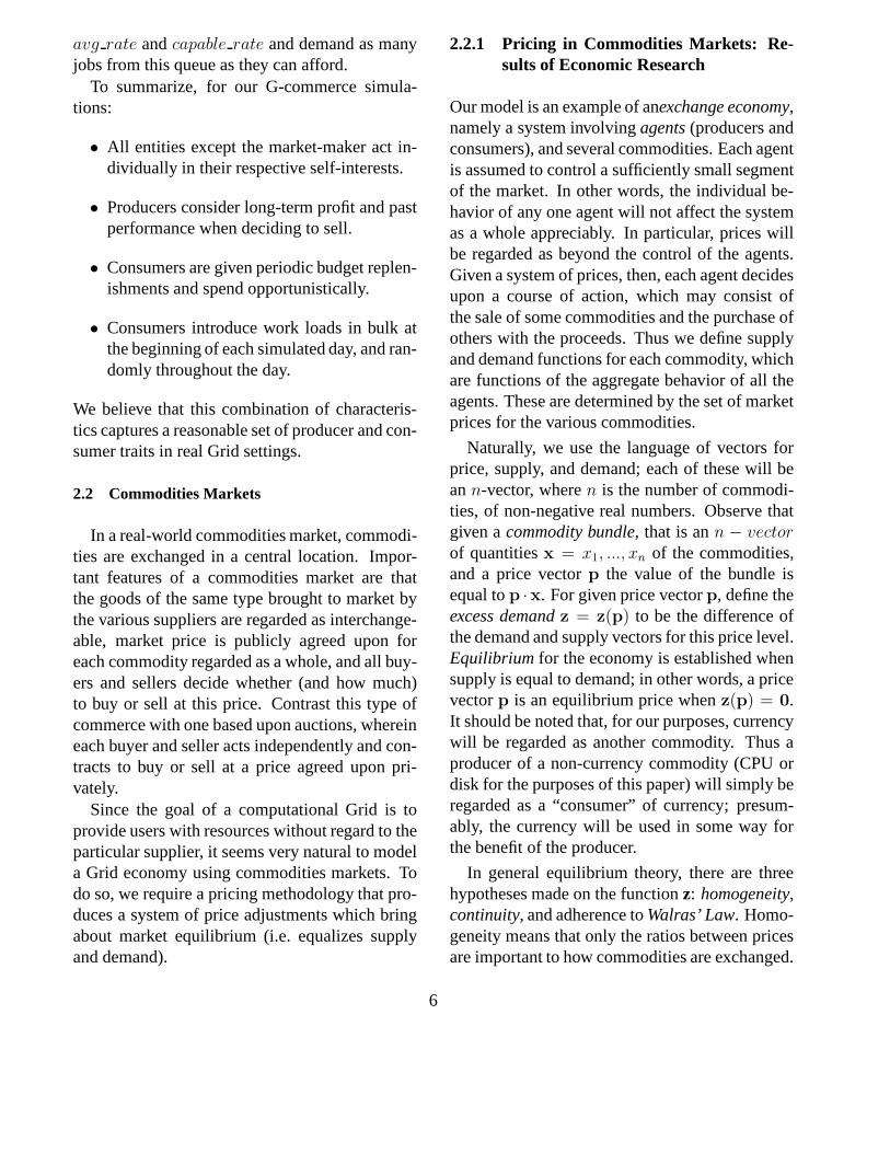
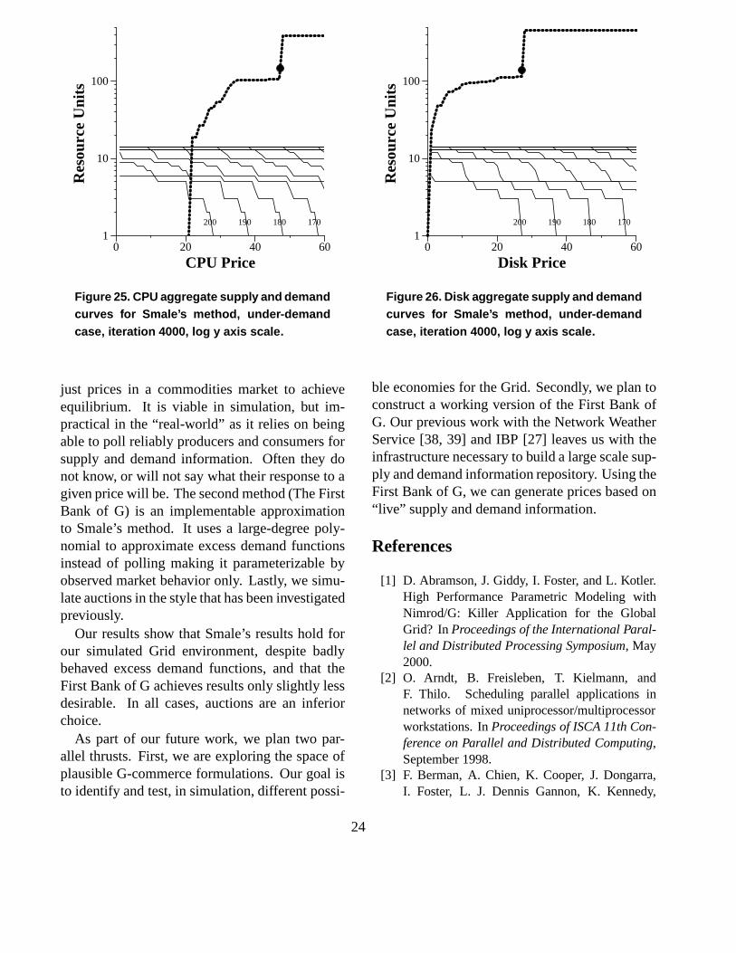
However, once the consumers’ jobs for the daybecome serviced, the system enters an under-demanded state. Consumers get new jobs at anaverage rate of one every ten time steps, and theytypically have plenty of $G with which to servicejobs. Producers on the other hand, are mostly idle.However, since they base their supply functionson average profit, they still refuse to sell until acertain threshold price is met. The state of the sys-tem during iteration 4000 is plotted in Figures 23and 24, using the same linear scale for the y-axesas in the other graphs, and in Figures 25 and 26,
20

0100
200300
400500
0
100
200
300
400
5000
10
20
30
40
50
60
Disk Price
Bank of Smale, over−demand case
CPU Price
Tot
al A
bsol
ute
Exc
ess
Dem
and
Figure 19. Total absolute excess demand min-ima, Smale’s Method, overdemand case. Theprojection upon the price plane is also shown.Filed circles represent equilibrium price solu-tions at this iteration.
using a more readable log scale.
Although it is difficult to discern from the fig-ures, there is no equilibrium point for both com-modities in this graph. This is because the systemat this point is not a well-behaved economy, sincethe lowering of prices does not necessarily bringabout an increase in demand. Put another way, thedemand is so low that the assumption that individ-ual agents do not make a significant difference isviolated. Regardless, both Smale’s method andthe Bank of G default to a “normal” price. Themarket is not cleared – there is a supply glut –but prices do not become abnormally depressed.These results indicate that both Smale’s methodand the First Bank of G will be reasonably ro-bust with respect to degeneration in the underly-ing economic behavior of the systems to whichthey are applied.
Probing further, the behavior of the banks inthis case can be accounted for by looking at thesupply and demand curves; note that the price thateach bank finds is one where the supply curve isalmost vertical and the demand curve horizontal,indicating a large jump in producer behavior at or
0100
200300
400500
0
100
200
300
400
5000
20
40
60
80
100
120
Disk Price
Bank of G, over−demand case
CPU Price
Tot
al A
bsol
ute
Exc
ess
Dem
and
Figure 20. Total absolute excess demand min-ima, Bank of G, overdemand case.
near this price. This means that the excess de-mand function for each commodity will locallydepend only on that commodity’s price and willbe extremely sensitive to small changes in price.Thus the Jacobian matrixDz(p) will have theform
very large 0negative number
very large0 negative number
The large diagonal entries will produce extremelysmall values of∆p for either price-adjustmentscheme. Note in this case that Smale’s methodreduces totatonnement(Cf. Section 2.2.1) due tothe off-diagonal zeros.
It is reasonable to expect that in more realis-tic simulations where true market behavior holds,and in any meaningful implementation of eitherof these price adjustment schemes, the behaviorof the agents will be sufficiently heterogeneous asto preclude the existence of such large jumps incumulative supply.
3.5 Efficiency
While commodities markets using Smale’smethod of price determination appear to offer bet-
21

0 50 100
CPU Price
0
50
100
150
Res
ourc
e U
nits
60708090
100
110
120
130
140
150
160
170
Price of Disk
Disk P
rice 65.52
Figure 21. CPU aggregate supply and demandcurves for Smale’s method, under-demandcase, iteration 3119.
ter theoretical and simulated economic properties(equilibrium and price stability) than auctions do,we also wish to consider the effect of the twopricing schemes on producer and consumer effi-ciency. To do so, we report the average percent-age of time each resource is occupied as a utiliza-tion metric for suppliers, and the average numberof jobs/minute each consumer was able to com-plete as a consumer metric. Table 2 summarizesthese values for both the over- and under-demandcases.
In terms of efficiency, Smale’s method is bestand the First Bank of G achieves almost the sameresults. Both are significantly better than the auc-tion in all metrics except disk utilization in theover-demanded case. Since CPUs are the scarceresource, disk price may fluctuate through a smallrange without consequence when lack of CPUsupply throttles the system. The auction seems toachieve slightly better disk utilization under theseconditions. In general, however, Smale’s methodand the First Bank of G approximation both out-
0 50 100
Disk Price
0
50
100
150
Res
ourc
e U
nits
60708090
100
110
120
130
140
150
160
170
Price of CPU
CP
U P
rice 119.27
Figure 22. Disk aggregate supply and demandcurves for Smale’s method, under-demandcase, iteration 3119.
perform the auction in the simulated Grid setting.
4 Conclusions and Future Work
In this paper, we investigate G-commerce —computational economies for controlling resourceallocation Computational Grid settings. We de-fine hypothetical resource consumers (represent-ing users and Grid-aware applications) and re-source producers (representing resource ownerswho “sell” their resources to the Grid). Whilethere are an infinite number of ways to representindividual resource supply and demand in simu-lated setting, and none are completely accurate,we have identified a set of traits that we believeare realistic.
• All entities except the market-maker act in-dividually in their respective self-interests.
• Producers consider long-term profit and pastperformance when deciding to sell.
22

efficiency metric under-demand over-demand
Smaleconsumer jobs/min 0.14 j/m 0.05 j/mB of G consumer jobs/min 0.13 j/m 0.04 j/mauction consumer jobs/min 0.07 j/m 0.03 j/m
SmaleCPU utilization % 60.7% 98.2%B of G CPU utilization % 60.4% 93.9%auctionCPU utilization % 35.2% 85.5%
Smaledisk utilization % 54.7% 88.3%B of G disk utilization % 54.3% 84.6%auctiondisk utilization % 37.6% 85.1%
Table 2. Consumer and Producer efficiencies
0 20 40 60
CPU Price
0
100
200
300
400
500
Res
ourc
e U
nits
Figure 23. CPU aggregate supply and demandcurves for Smale’s method, under-demandcase, iteration 4000.
• Consumers are given periodic budget replen-ishments and spend opportunistically.
• Consumers introduce work loads in bulk atthe beginning of each simulated day, and ran-domly throughout the day.
Using simulated consumers and producersobeying these constraints, we investigate twomarket strategies for setting prices: commodi-ties markets and auctions. Commodities mar-
0 20 40 60
Disk Price
0
100
200
300
400
500
Res
ourc
e U
nits
Figure 24. Disk aggregate supply and demandcurves for Smale’s method, under-demandcase, iteration 4000.
kets are a natural choice given the fundamen-tal tenets of the Grid [17]. Auctions, however,are simple to implement and widely studied. Weare interested in which methodology is most ap-propriate for Grid settings. To investigate thisquestion, we examine the overall price stability,market equilibrium, producer efficiency, and con-sumer efficiency achieved by three methods insimulation. The first implements the theoreticalwork of Smale [33] which describes how to ad-
23
0 20 40 60
CPU Price
1
10
100R
esou
rce
Uni
ts
200 190 180 170
Figure 25. CPU aggregate supply and demandcurves for Smale’s method, under-demandcase, iteration 4000, log y axis scale.
just prices in a commodities market to achieveequilibrium. It is viable in simulation, but im-practical in the “real-world” as it relies on beingable to poll reliably producers and consumers forsupply and demand information. Often they donot know, or will not say what their response to agiven price will be. The second method (The FirstBank of G) is an implementable approximationto Smale’s method. It uses a large-degree poly-nomial to approximate excess demand functionsinstead of polling making it parameterizable byobserved market behavior only. Lastly, we simu-late auctions in the style that has been investigatedpreviously.
Our results show that Smale’s results hold forour simulated Grid environment, despite badlybehaved excess demand functions, and that theFirst Bank of G achieves results only slightly lessdesirable. In all cases, auctions are an inferiorchoice.
As part of our future work, we plan two par-allel thrusts. First, we are exploring the space ofplausible G-commerce formulations. Our goal isto identify and test, in simulation, different possi-
0 20 40 60
Disk Price
1
10
100
Res
ourc
e U
nits
200 190 180 170
Figure 26. Disk aggregate supply and demandcurves for Smale’s method, under-demandcase, iteration 4000, log y axis scale.
ble economies for the Grid. Secondly, we plan toconstruct a working version of the First Bank ofG. Our previous work with the Network WeatherService [38, 39] and IBP [27] leaves us with theinfrastructure necessary to build a large scale sup-ply and demand information repository. Using theFirst Bank of G, we can generate prices based on“live” supply and demand information.
References
[1] D. Abramson, J. Giddy, I. Foster, and L. Kotler.High Performance Parametric Modeling withNimrod/G: Killer Application for the GlobalGrid? InProceedings of the International Paral-lel and Distributed Processing Symposium, May2000.
[2] O. Arndt, B. Freisleben, T. Kielmann, andF. Thilo. Scheduling parallel applications innetworks of mixed uniprocessor/multiprocessorworkstations. InProceedings of ISCA 11th Con-ference on Parallel and Distributed Computing,September 1998.
[3] F. Berman, A. Chien, K. Cooper, J. Dongarra,I. Foster, L. J. Dennis Gannon, K. Kennedy,
24

C. Kesselman, D. Reed, L. Torczon, , andR. Wolski. The grads project: Software sup-port for high-level grid application development.Technical Report Rice COMPTR00-355, RiceUniversity, February 2000.
[4] F. Berman, R. Wolski, S. Figueira, J. Schopf,and G. Shao. Application level scheduling ondistributed heterogeneous networks. InProceed-ings of Supercomputing 1996, 1996.
[5] J. Bredin, D. Kotz, and D. Rus. Market-basedResource Control for Mobile Agents. Techni-cal Report PCS-TR97-326, Dartmouth College,Computer Science, Hanover, NH, Nov. 1997.
[6] J. Bredin, D. Kotz, and D. Rus. Market-based re-source control for mobile agents. InSecond In-ternational Conference on Autonomous Agents,pages 197–204. ACM Press, May 1998.
[7] J. Bredin, D. Kotz, and D. Rus. Utility drivenmobile-agent scheduling. Technical ReportPCS-TR98-331, Dartmouth College, ComputerScience, Hanover, NH, October 1998.
[8] H. Casanova and J. Dongarra. NetSolve: A Net-work Server for Solving Computational ScienceProblems. The International Journal of Super-computer Applications and High PerformanceComputing, 1997.
[9] H. Casanova, G. Obertelli, F. Bermand, andR. Wolski. The AppLeS Parameter Sweep Tem-plate: User-Level Middleware for the Grid. InProceedings of SC00, November 2000. to ap-pear.
[10] J. Q. Cheng and M. P. Wellman. The WALRASalgorithm: A convergent distributed implemen-tation of general equilibrium outcomes.Compu-tational Economics, 12:1–24, 1998.
[11] B. Chun and D. E. Culler. Market-basedproportional resource sharing for clus-ters. Millenium Project Research Report,http://www.cs.berkeley.edu/˜plink/papers/market.pdf , Sep 1999.
[12] B. N. Chun and D. E. Culler. Market-based pro-portional resource sharing for clusters. Mille-nium Project Research Report, Sep. 1999.
[13] G. Debreu. Theory of Value. Yale UniversityPress, 1959.
[14] B. C. Eaves. Homotopies for computation offixed points. Mathematical Programming, 3:1–22, 1972.
[15] B. Ellickson. Competitive Equilibrium: Theoryand Applications. Cambridge University Press,1993.
[16] I. Foster and C. Kesselman. Globus: A meta-computing infrastructure toolkit.InternationalJournal of Supercomputer Applications, 1997.
[17] I. Foster and C. Kesselman.The Grid: Blueprintfor a New Computing Infrastructure. MorganKaufmann Publishers, Inc., 1998.
[18] I. Foster, A. Roy, and L. Winkler. A qualityof service architecture that combines resourcereservation and application adaptation. InPro-ceedings of TERENA Networking Conference,2000. to appear.
[19] J. Gehrinf and A. Reinfeld. Mars - a frameworkfor minimizing the job execution time in a meta-computing environment.Proceedings of Futuregeneral Computer Systems, 1996.
[20] A. S. Grimshaw, W. A. Wulf, J. C. French, A. C.Weaver, and P. F. Reynolds. Legion: The nextlogical step toward a nationwide virtual com-puter. Technical Report CS-94-21, University ofVirginia, 1994.
[21] J. M. M. Ferris, M. Mesnier. Neos and condor:Solving optimization problems over the inter-net. Technical Report ANL/MCS-P708-0398,Argonne National Laboratory, March 1998.http://www-fp.mcs.anl.gov/otc/Guide/TechReports/index.html .
[22] A. Mas-Colell.The Theory of General EconomicEquilibrium: A Differentiable Approach. Cam-bridge University Press, 1985.
[23] O. H. Merrill. Applications and extensions of analgorithm that computes fixed points of certainupper semi-continuous point to set mappings.Ph.D. Dissertation, Dept. of Ind. Engineering,University of Michigan, 1972.
[24] H. Nakada, H. Takagi, S. Matsuoka, U. Na-gashima, M. Sato, and S. Sekiguchi. Utiliz-ing the metaserver architecture in the ninf globalcomputing system. InHigh-Performance Com-puting and Networking ’98, LNCS 1401, pages607–616, 1998.
[25] N. Nisan, S. London, O. Regev, and N. Camiel.Globally distributed computation over the Inter-net — the POPCORN project. InInternationalConference on Distributed Computing Systems,1998.
25

[26] N. N. Ori Regev. The popcorn market - an onlinemarket for computational resources. First Inter-national Conference On Information and Com-putation Economies. Charleston SC, 1998. Toappear.
[27] J. Plank, M. Beck, and W. Elwasif. IBP: Theinternet backplane protocol. Technical ReportUT-CS-99-426, University of Tennessee, 1999.
[28] B. Rajkumar. Ecogrid home pagehttp://www.csse.monash.edu.au/˜rajkumar/ecogrid/index.html .
[29] B. Rajkumar. economygrid home pagehttp://www.computingportals.org/projects/economyManager.xml.html .
[30] H. Scarf. Some examples of global instability ofthe competitive equilibrium.International Eco-nomic Review, 1:157–172, 1960.
[31] H. Scarf. The Computation of Economic Equi-libria . Yale University Press, 1973.
[32] S. Smale. Price adjustment and global Newtonmethods. Frontiers of Quantitative Economics,IIIA:191–205, 1975.
[33] S. Smale. Dynamics in general equilibrium the-ory. American Economic Review, 66(2):284–294, May 1976.
[34] T. Tannenbaum and M. Litzkow. The condor dis-tributed processing system.Dr. Dobbs Journal,February 1995.
[35] C. A. Waldspurger, T. Hogg, B. Huberman, J. O.Kephart, and S. Stornetta. Spawn: A distributedcomputational economy.IEEE Transactions onSoftware Engineering, 18(2):103–117, February1992.
[36] C. A. Waldspurger, T. Hogg, B. A. Huberman,J. O. Kephart, and W. S. Stornetta. Spawn:A distributed computational economy.IEEETrans. on Software Engineering, 18(2):103–117,February 1992.
[37] L. Walras.Elements d’Economie Politique Pure.Corbaz, 1874.
[38] R. Wolski. Dynamically forecasting networkperformance using the network weather service.Cluster Computing, 1998. also available fromhttp://www.cs.utk.edu/ rich/publications/nws-tr.ps.gz.
[39] R. Wolski, N. Spring, and J. Hayes. The net-work weather service: A distributed resourceperformance fore casting service for metacom-puting. Future Generation Computer Sys-tems, 15(5-6):757–768, October 1999. availablefrom http://www.cs.utk.edu/˜rich/publications/nws-arch.ps.gz .
26