anatomy of performance fees in finnish mutual funds
TRANSCRIPT

Anatomy of performance fees in Finnish mutual funds
Finance
Master's thesis
Timo Pohjanpalo
2013
Department of FinanceAalto UniversitySchool of Business
Powered by TCPDF (www.tcpdf.org)

Anatomy of performance fees in
Finnish mutual funds
Master’s Thesis
Timo Pohjanpalo
Fall 2013
Finance
Approved in the Department of Finance __ / __20__ and awarded the grade
_______________________________________________________

Aalto University, P.O. BOX 11000, 00076
AALTO
www.aalto.fi
Abstract of master’s thesis
Author Timo Pohjanpalo
Title of thesis Anatomy of performance fees in Finnish mutual funds
Degree Master of Science in Business Administration
Degree programme Finance
Thesis advisor(s) Professor Matti Keloharju
Year of approval 2013 Number of pages 81 Language English
OBJECTIVES OF THE STUDY
In this thesis, I study the use of performance fees in Finnish mutual funds, their impact on the funds’ risk-adjusted return, risk and their theoretical value. Furthermore, utilizing simulation-based methods, my objective is to calculate a theoretical value for the performance fee structures in Finnish mutual funds. Finally, I also study the different regulatory approaches to performance fees in select European countries and the disclosure of Finnish funds’ performance fees.
DATA AND METHODOLOGY
My sample consists of 332 mutual funds registered in Finland and contains quarterly observations on each fund from March 2007 to December 2012. 40 of these funds utilize performance fees. The sample is free from survivorship bias. My analysis is primarily based on random effects panel regressions with a variety of risk and return variables as dependent variables and funds’ individual characteristics as explanatory variables. I also utilize Monte Carlo simulation and the Margrabe model to calculate the cost of the fee for each of the funds in the sample.
FINDINGS OF THE STUDY
Funds with performance fees offer better risk-adjusted returns. The introduction of a performance fee increases the funds’ ex post four-factor alpha by on average 83 basis points per quarter. The results hold also when using Sharpe ratio and the raw quarterly return as dependent variables. The use of performance fees does not increase funds’ volatility levels relative to funds without such fees. However, funds with performance fees exhibit higher tracking errors, implying that funds take more active risk compared to their counterparts.
The theoretical value of the performance fee is on average 1.35% Furthermore, funds with performance fees, on average, offer significantly lower management and redemption fees than funds without such fee structures. The difference is 22 and 24 basis points p.a. for management and redemption fees, respectively. However, the extra cost associated with the performance fees makes these funds more expensive on an annual basis.
Keywords performance fee, incentive fee, risk-adjusted return, incentives, mutual funds, fund
management, principal-agent problem, simulation, spread option, principal-agent problem

Aalto University, P.O. BOX 11000, 00076
AALTO
www.aalto.fi
Gradutiivistelmä
Tekijä Timo Pohjanpalo
Otsikko: Tuottosidonnaiset palkkiot suomalaisissa sijoitusrahastoissa
Tutkinto Kauppatieteiden maisteri
Ohjelma Rahoitus
Ohjaaja Professori Matti Keloharju
Hyväksytty 2013 Sivumäärä 81 Kieli Englanti
TUTKIELMAN TAVOITTEET
Tutkin pro gradu-tutkielmassani tuottosidonnaisten palkkioiden käyttöä suomalaisissa sijoitusrahastoissa, niiden vaikutusta tuottoon ja riskiin. Lisäksi lasken palkkiorakenteiden teoreettisen arvon jokaisella kyseistä palkkiota käyttävälle suomalaiselle rahastolle. Lisäksi tutkin erilaisia regulatorisia lähestymistapoja tuottosidonnaisten palkkioiden suhteen sekä suomalaisten tuottosidonnaisten palkkioiden julkituontia.
DATA JA METODOLOGIA
Otokseni koostuu 332 Suomeen rekisteröidystä sijoitusrahastosta ja neljännesvuosittaisista havainnoista aikavälillä maaliskuusta 2007 joulukuuhun 2012. Otoksen rahastoista 40:ssä on tuottosidonnainen palkkio. Otos ei kärsi selviytymisvinoumasta. Analyysini perustuu satunnaisvaikutuspaneeliregressioon hyödyntäen useita erilaisia riski – ja tuottomuuttujia. Hyödynnän lisäksi Monte Carlo-simulaatiota sekä Margraben mallia tuottosidonnaisen palkkiorakenteen teoreettisen arvon määrittämiseen jokaiselle rahastolle otoksessani.
TULOKSET
Tuottosidonnaisia palkkioita käyttävät rahastot tarjoavat parempia riskikorjattuja tuottoja. Tuottosidonnaisen palkkion käyttö lisää ex post neljän muuttujan riskikorjattua tuottoa 83 korkopistettä kvartaalissa. Tulokset ovat samanlaisia myös käytettäessä Sharpen suhdelukua sekä riskikorjaamatonta tuottoa riippuvana muuttujana. Tuottosidonnaiset palkkiot eivät lisää rahastojen absoluuttista riskiä volatiliteetillä mitattuna. Tuottosidonnaista palkkiota käyttävät rahastot kuitenkin ottavat enemmän riskiä seurantavirheellä mitattuna.
Tuottosidonnaisen palkkion teoreettinen arvo on keskimäärin 1.35% p.a.. Lisäksi tuottosidonnaista palkkiota käyttävien rahastojen hallinnointi – ja lunastuspalkkio ovat 22 ja 24 korkopistettä alhaisempia normaaleihin rahastoihin verrattuna. Kokonaiskustannuksiltaan tuottosidonnaista palkkiota käyttävät rahastot ovat kuitenkin normaaleja rahastoja kalliimpia.
Avainsanat: tuottosidonnainen palkkio, riskikorjattu tuotto, kannusteet, sijoitusrahastot, agentti-
päämiesongelma, simulaatio, optio

I "PRESS HERE TO SAVE"
TABLE OF CONTENTS
1. Introduction ........................................................................................................................ 1
1.1. Contribution to existing research ................................................................................. 3
1.2. Key research questions ................................................................................................ 4
1.3. Main findings ............................................................................................................... 6
1.4. Limitations of the study ............................................................................................... 7
1.5. Structure of thesis ........................................................................................................ 9
1.6. Definitions ................................................................................................................... 9
2. Literature review .............................................................................................................. 11
2.1. Principal-agent problems in delegated portfolio management .................................. 11
2.2. Impact of performance fees on fund returns .............................................................. 15
2.3. Performance fees and fund management behaviour .................................................. 16
2.4. Other implicit disciplinary mechanisms for fund management ................................. 19
2.5. Valuation of the performance fee option ................................................................... 20
3. Regulatory approaches to performance fees in Europe and the U.S. ............................... 21
3.1. Common principles from the UCITS IV directive and the IOSCO .......................... 21
3.2. National approaches used by European and U.S. regulators ..................................... 22
3.3. Finnish mutual funds and the IOSCO guidelines ...................................................... 27
4. Hypotheses ....................................................................................................................... 28
4.1. Performance fees and fund return .............................................................................. 28
4.2. Performance fees and fund risk ................................................................................. 29
5. Data .................................................................................................................................. 30
5.1. Overview of data used in research and data gathering .............................................. 30
5.2. Performance fees in Finnish mutual funds ................................................................ 33
5.3. Calculation of raw returns and risk-adjusted returns ................................................. 35
5.3.1. Quarterly raw returns ......................................................................................... 35
5.3.2. Categorization of funds for calculation of risk-adjusted returns ........................ 36
5.3.3. Explanatory portfolios used for risk-adjustment ................................................ 36
5.3.4. Calculation of risk-adjusted returns ................................................................... 37
5.4. Tracking error data and calculations ......................................................................... 39
6. Analysis and results .......................................................................................................... 41
6.1. Performance fees and fund returns ............................................................................ 41
6.1.1. Impact of performance fees on funds’ raw, non-risk-adjusted returns .............. 41
6.1.2. Impact of performance fees on fund’s four-factor alpha .................................... 43
6.1.3. Impact of performance fees on a fund’s Sharpe ratio ........................................ 44
6.1.4. Summary of the impact of performance fees on funds’ risk-adjusted return ..... 45
6.2. Performance fees and fund management behaviour .................................................. 46
6.2.1. Performance fees and volatility levels ............................................................... 47
6.2.2. Differences in tracking error .............................................................................. 49
6.2.3. Summary of performance fees and fund management behaviour ...................... 51
6.3. Valuation of the performance fee option ................................................................... 51
6.3.1. Introduction to the valuation of the performance fee ......................................... 51
6.3.2. Conducting the simulation-based valuation of performance fees ...................... 56 6.3.2.1 Simulation of fund and benchmark price paths ......................................................... 56

II "PRESS HERE TO SAVE"
6.3.2.1 Calculation of payoffs from the performance fee option .......................................... 57
6.3.3. Results of the valuation of performance fees ..................................................... 58
6.3.4. Sensitivity of results to changes in key parameters ............................................ 60
6.4. Performance fees in relation to other fund fees ......................................................... 61
6.4.1. Comparison of fixed fees between fund types ................................................... 61
7. Discussion of results......................................................................................................... 64
7.1. Regulatory implications ............................................................................................. 65
7.2. Economic implications .............................................................................................. 66
8. Conclusions ...................................................................................................................... 67
REFERENCES ......................................................................................................................... 70
APPENDIX A. Compliance of Finnish funds with IOSCO recommendations ....................... 73
APPENDIX B. Overview of funds in the sample utilizing performance fees ......................... 75
APPENDIX C. Overview of quarterly returns of explanatory portfolios ................................ 76
APPENDIX D. Summary statistics on the subsample for tracking error calculations ............ 77
APPENDIX E. Sensitivity analysis ......................................................................................... 78
APPENDIX F. Individual results of the valuation .................................................................. 79
LIST OF TABLES
Table 1: Definition of key terms used in the thesis .................................................................... 9
Table 2: Summary of different regulatory approaches to performance fees ............................ 23
Table 3: Overview of the sample ............................................................................................. 31
Table 4: Correlation matrix of key variables ........................................................................... 32
Table 5: Summary of performance fees charged by mutual funds in the sample .................... 34
Table 6: Estimated quarterly ex post four-factor alphas of the funds in the sample ................ 39
Table 7: Raw quarterly returns and fund characteristics .......................................................... 42
Table 8: After-fee four-factor alphas and fund characteristics ................................................ 43
Table 9: Annual Sharpe ratio and fund characteristics ............................................................ 45
Table 10: Use of performance fees and mutual fund volatility ................................................ 49
Table 11: Differences in tracking errors .................................................................................. 50
Table 12: Ex ante value of the performance fees of Finnish mutual funds .............................. 59
Table 13: Differences in average fees of funds with performance fees and without ............... 62
Table 14: Summary of empirical findings ................................................................................ 64
Table 15: Quarterly returns of the explanatory portfolios 03/2007-12/2012 ........................... 76
Table 16: Sensitivity analysis of performance fees .................................................................. 78
Table 17: Individual valuation results and key assumptions .................................................... 79
LIST OF FIGURES
Figure 1: Distribution of participation rates in Finnish funds with performance fees ............. 35
Figure 2: Illustration of the use of high-water marks ............................................................... 52
Figure 3: Cumulative distribution of performance fees’ ex ante values .................................. 59
Figure 4: Sensitivity of fee values to changes in correlation and volatility ............................. 60
Figure 5: Total cost of average fund with performance fee ..................................................... 63
1
1. Introduction
“These funds [with performance fees] effectively charge a performance fee for winning the lottery. If they base the fee on a track record that depends as much on chance, you are paying for luck as much as skill.” – (Rick Di Mascio, former pension fund manager, Financial Times, July 22nd 2011)
“I believe there is no need for performance fees within open funds. If assets grow and the fund earns more as a result of good performance, then that is fair. But ways of stealing profits from investors should be phased out.” – (Sven Gielod, Member of the European Parliament, Financial Times, November 18th 2012)
Mutual funds charge their owners various fees, which have been under intense scrutiny in the
past years both in academia and the financial press. The direct and indirect fees incurred by
fund owners have a large impact on their net return. Furthermore, the justification for
charging fees, especially performance fees, which are the focus of this thesis, is at time
heavily contested. As evidenced by the quotes above, politicians and investment management
professionals often have passionate opinions about performance fees and their fairness.
In general, the relationship between investors and fund managers can be seen as a direct
application of the traditional principal-agent relationship, in which the principal (the investor)
gives control over her wealth to the agent (the fund manager). As is always the case with a
principal-agent relationship, mutual funds suffer from an inherent conflict of interest due to
the fact that the interests of the parties in the relationship are not aligned. In mutual funds, the
agent (fund management) has a different incentive compared to the principal (fund investors).
Simplistically, the fund management strives to maximize the value of their own income,
which primarily consists of fees charged from the investors, whereas the fund holders simply
want to maximize the return on their investment at a certain level of risk tolerance.
One special type of funds’ fees is a fee type called the performance fee, in which the fund
management gets a certain portion of returns exceeding the return of a preset benchmark. In
principle, this type of incentive structure ought to reduce the aforementioned conflicts of
interest between fund management and investors, as the performance fee gives the
management an explicit incentive to maximize fund returns. However, as I elaborate later on,
this incentivization to maximize returns may lead to undesired consequences such as excess
risk-taking.
In this thesis, I study the use of performance fees in Finnish mutual funds, their impact on the
risk and return of the funds and their theoretical value to the fund management. The existing
research on the topic has been scarce most likely due to the fact that in 1970 an amendment to

2
the Investment Company Act, the United States congress prevented mutual funds from
charging asymmetric (i.e. fees, where the management shares the upside, but not the
downside) performance fees (Thomas and Jaye, 2006). Only a few managers have been
confident enough to charge so-called fulcrum (i.e. symmetric) performance fees, (Drago et al.,
2010), which decrease the management fee when the fund underperforms the benchmark.
Naturally, to claim that fund managers solely maximize their own fees with no regard to fund
performance is an oversimplification, as there are also other forces in play. The investors have
a variety of means to discipline the fund managers, namely by voting with their feet and
leaving the fund in case of poor performance. The flow-performance relationship in which
mutual fund inflows and outflows directly follow fund performance has been widely
documented in literature (see e.g. Berk and Green, 2002 and Huang et al., 2007) The flow-
performance relationship can thus be seen as an implicit incentive contract. The existence of
this disciplinary mechanism implicitly incentivizes the fund management to operate at least
partly in the interest of the investors, as otherwise investors will withdraw their investment,
consequently reducing the fund management’s income from the fixed fees.
Furthermore, as noted by Chevalier and Ellison (1999), the long-term career concerns of
mutual fund managers also give the management an incentive to deliver returns to investors
even without the existence of explicit contractual incentive mechanisms. Managers
consistently squandering investors’ money can expect to see the number of investment
management job opportunities diminish, especially considering the intense media scrutiny
fund managers are subject to.
However, despite the aforementioned caveats, performance fees’ impact on risk and return
characteristics of specifically mutual funds provides a fascinating research topic, given their
importance as investment vehicles for retail investors and openness and the relatively low
amount of existing empirical research on the topic. Furthermore, contrary to the implicit
incentives mentioned above, performance fees are an explicit, simple mechanism designed to
achieve one thing: higher returns. Thus, the functionality of this incentive mechanism
provides a fascinating area of study.
The topic of performance fees is especially interesting, when one looks at the performance
fees as an explicit option held by the management written by the investors. The theoretical
value of the performance fee can be calculated by treating the fee as if the management has a

3
call option on a certain fraction (participation rate) of the spread between fund and benchmark
returns multiplied by fund assets under management (Kritzman, 1987). Consequently, option
valuation techniques such as extensions to the Black-Scholes-Merton model and numerical
methods can be applied to attempt to estimate the monetary value of the option held by the
management.
Moreover, the option-valuation reasoning enables some simple empirical tests to see whether
there are any implications of self-interested behaviour on the part of managers of funds with
performance fees. For instance, the value of performance fees is positively related to the
tracking error of the fund. Assuming that fund managers maximize the value of their fee
income, we should, ceteris paribus, observe higher tracking errors for funds using
performance fees, as higher tracking errors increase the value of the option (Elton et al.,
2003).
1.1. Contribution to existing research
My thesis contributes to existing research in a variety of ways. Firstly, even though the area of
mutual fund returns and fees has been very extensively researched, the area of performance
fees in mutual funds is not equally well known (For existing key research, see for example
Elton et al., 2003; Golec, 1988 and Massa and Patgiri, 2009). One of the reasons for the
relative lack of research on performance fees in mutual funds is the fact that due to the
Investment Company Act of 1970, U.S. mutual funds have been prohibited from charging
asymmetric incentive fees, which has effectively limited research on the topic to non-U.S.
countries only.
Consequently, finding out more about the relationship between performance fees and mutual
fund returns and risk in a Finnish context is an intriguing question with practical significance
to both retail investors and the academic world that is yet to be answered in previous research.
In Finland, the share of holdings in funds with performance fees has steadily increased during
the last decade from 2% in 2004 to 4.3% in 2008 with performance fee funds being favored
by wealthier and more educated investors (Keloharju et al., 2012).

4
Furthermore, the spread option valuation approach to performance fees has, to the best of my
knowledge, only been utilized done once in an unfinished working paper1 by Drago et al.
(2005). Moreover, Kritzman (1987) utilized the Magrabe model (see Margrabe, 1978) to
arrive at a monetary value for the performance fees in a simplistic setting. In the field of
hedge funds, Goetzmann et al. (2003) provide some estimates for theoretical values for hedge
fund incentive contracts.
However, apart from studies mentioned above, there are, to the best of my knowledge, no
other studies attempting to calculate a monetary value for performance fees for mutual funds.
Thus, there is a clear gap in existing research which my study partly attempts to fill by
calculating the ex ante value of the performance fee options utilizing Finnish data. The
advantage of my approach, in which I calculate the theoretical value of the performance fee
for each Finnish fund separately, is that it gives a tangible, generalizable estimate for the
actual cost of performance fees in Finnish funds using actual return data, volatilities and
correlations.
In addition to filling the existing research gap on the value of performance fees and their
relation to mutual funds’ return and risk, my research also has practical significance to retail
investors. Mutual funds are one of the key investment vehicles available for use to retail
investors. However, retail investors often lack the financial sophistication to be able to
holistically evaluate and compare funds, especially involving mathematically complex and
opaque components such as performance fees. Thus, researching performance fees in a
mutual fund context adds value to the investment decision process for retail investors.
1.2. Key research questions
My study can be divided into three high-level categories. First, I test the impact of
performance fees’ impact on fund risk and return empirically. Second, I calculate a theoretical
value for the performance fees and compare the costs of funds with performance fees to funds
without such structures. Thirdly, I provide some context for the regulation of performance
fees by describing the regulatory approach to fees in select European countries.
1 To be more exact, the final paper was published in Financial Management, but from a completely different perspective not including the performance fee valuation. I contacted Professor Navone to enquire about the matter and the reason the original paper was never published was related to the journal’s referees’ low interest in the value of the fees, as a consequence of which the focus of the paper was altered. Due to this reason, I often refer to the working paper version of the article instead of the finished, published article, which is of lower relevance to my research.

5
Performance fees can be seen as a contractual mechanism that align interests of fund
managers and investors more closely and incentivize the fund management to utilize their
skills to provide higher returns. This argument leads me to my first research question:
I. Research question: What is the impact of performance fees on fund returns in
Finland?
Following along with the option valuation approach, another question arises: as the ex ante
value of a performance fee increases along with the volatility of the mutual fund and the
tracking error, I would expect to observe higher active and absolute risk-levels for funds with
performance fees.
II. Research question: Do funds with performance fees on average exhibit more risk in
terms of volatility, when adjusted for differences in investment styles?
III. Research question: Do funds with performance fees exhibit on average higher
tracking errors?
Furthermore, from a contextual perspective, the costs of performance fees are not obvious to
the layman and it is, from the retail investors’ point of view, an additional cost component.
Thus, estimating an explicit theoretical value for the performance fee provides an interesting
research question.
IV. Research question: What is the cost of these performance fees as a percentage of fund
AUM?
A logical extension to the above question is whether funds with performance fees end up
being cheaper, equally costly or more expensive to investors. Furthermore, if the performance
fees are indeed an extra cost to the investors, it is interesting to see whether the investors are
compensated for the extra cost.
V. Research question: Do Finnish funds with performance fees charge lower other
expenses compared to funds without extra fees? How do the total costs, including the
calculated value of the performance fee, of funds with performance fees compare to
funds without such fees?

6
Furthermore, the use and regulation of performance fees varies notably in Europe. In order to
form a holistic picture on the regulatory drivers behind performance fees, I conduct some
descriptive analysis on the different regulatory regimes with regards to performance fees and
attempt to find out whether there are any differences across different countries.
VI. Research question: How does the regulatory approach to performance fees differ in
select European countries and the United States?
1.3. Main findings
My dataset consists of 332 Finnish mutual funds with quarterly observations from March
2007 to December 2012. The dataset has been acquired via requests from Morningstar and
Investment Research Finland, complemented by manual data gathering from individual fund
prospectuses and rules.
The key finding of my study is that the introduction of a contractual performance fees has a
positive impact on a fund’s risk-adjusted return, even after controlling for time and
investment style factors. The impact is 82 basis points per quarter on a fund’s four-factor
alpha. The result is highly significant. The positive relationship between the use of
performance fees and fund returns is observed also when using different dependent variables
such as raw returns and the Sharpe ratio.
The extra risk-adjusted return does not seem to be associated with additional volatility. When
controlling for time effects and lagged volatility, the coefficient for the performance fee
dummy is not significant. However, in terms of active risk, funds with performance fees do
seem to take more active risk in terms of tracking error, which measures the standard
deviation of the difference in returns of the fund and the benchmark. On average, funds with
performance fees have tracking errors which are 4.09 percentage points higher than funds
without performance fees. The difference is statistically significant, which implies that funds
with performance fees have a tendency to take more active risk by deviating from the
benchmark. This higher active risk can be achieved by taking positions in instruments either
not included in the benchmark or by deviating from the weights of the benchmark in the asset
allocation process.
Furthermore, I calculate the theoretical value individually for each of the 40 funds using
performance fees in my sample as of beginning of 2013.The theoretical value of performance

7
fees is on average 1.35% per annum of a fund’s assets under management at the beginning of
the calculation period. The standard deviation for the value is 1.01%. The maximum
performance fee in my sample is 4.84% whereas the lowest value is 0.01%. The estimated
value is highly sensitive to changes in key parameters such as volatility and correlation.
With regards to other fund fees, funds with performance fees offer lower management and
redemption fees to their investors, while there is no significant difference in subscription fees.
The discount to management and redemption fees is 22 and 24 basis points, respectively.
Thus, funds with performance fees seem to offer discounts from other fees to compensate for
the introduction of a performance fee. However, when including the calculated value of the
performance fee into the picture, funds with performance fees do appear to be more expensive
on a total cost basis.
1.4. Limitations of the study
The main limitations of the study are related to the actual details of the performance fees.
Despite the fact that fund prospectuses disclose the existence and calculation basis of the
performance fees, the level of detail in disclosure is at times relatively poor. Overall, based on
the fund prospectuses it is challenging to form a holistic, detailed picture of the performance
fees that is comparable across funds, as the variation in calculation methodologies and
disclosure is considerable. When available, I utilize all of the documentation available related
to funds (rules, Key Investor Information Document (KIID) and websites) to find out as much
as possible about the calculation mechanics of the performance fee.
One of the most significant limitations impacting the estimated value of the performance fee
is the magnitude of the utilized high-water mark. As the value for the high-water mark
changes across time, I opt to conduct the valuations at a single point in time, as of the
beginning of 2013. I acquire the high-water mark for each of the funds in the sample utilizing
the funds’ historical prices at the end of 2012. However, the value of the high-water mark
relative to the fund’s year-end value understandably varies considerably across funds,
consequently affecting the estimated value. To correct for this, I also calculate the value of the
performance fee assuming that the high-water mark is set at the initial value of the fund at the
beginning of a calculation period.
The variety of the investment styles of the funds in the sample also poses challenges to the
calculation of risk-adjusted returns. In order to conduct a robust risk-adjustment to the raw

8
returns of the funds in the sample, I require return data for explanatory portfolios for different
investment styles. For data availability reasons, I opt to group the funds in my sample into
five different geographical categories based on their investment focus. Consequently,
different geographical explanatory portfolios were used for the risk-adjustment. However, the
categorization of the funds into the five geographical categories does not always provide a
perfect match with the actual investment style. As a result of this, the risk-adjustment to the
raw returns may not always be completely accurate due to inherent differences in the fund
portfolio and the explanatory portfolio. To ensure the robustness of my results and to counter
for any erroneous categorizations in the risk-adjustment, I also run regressions on other
dependent variables such as the Sharpe ratio and the raw, non-adjusted return.
Furthermore, in cases where the performance fee is mathematically more complex (i.e.
containing high-water marks or positivity constraints), finding a closed-form solution is
impossible and numerical methods such as the binomial pyramid approach or Monte Carlo
simulation need to be used to approximate the value of the fee. However, the use of numerical
estimation methods is not a large limitation, as the simulated value of the fee converges to the
actual value as the number of simulations increases.
The calculation of the tracking errors and correlations also suffers from data availability
issues. As benchmark return data is not available for all of the funds in the sample from
sources at my disposal (primarily Bloomberg), I am forced to drop some of the funds for the
purposes of the tracking error calculations. In general, the dropped funds are generally
younger and have lower assets under management.
The option valuation approach also suffers from some methodological limitations. Firstly,
both the Margrabe (1978) model and basic form of the Monte Carlo simulation assume static
fund volatility and correlation with the benchmark. In reality, however, the fund management
has the opportunity to impact both of these factors in response to how much their performance
fee option is in/out the money. There are some empirical indications that portfolio managers
indeed do so (see e.g. Brown et al., 1996 and Huang et al. 2011). However, taking these
factors into account by attempting to model the dynamic correlation between the fund and the
benchmark and the changes in volatility is beyond the scope of this thesis.
In the comparison of total cost of ownership of funds with and without performance fees, I
take into account only the running annual costs (i.e. the management fee) of the fund for two

9
reasons. Firstly, taking into account the one-off subscription and redemption fees in the
comparison would require assumptions and/or data on the average holding period for each of
the funds to calculate the assumed yearly cost associated with these fees. The holding period
data is not available. Secondly, management fees represent the bulk of mutual fund
companies’ income and consequently investors’ costs, contrary to subscription fees and
redemption fees, which play a smaller role.
One additional aspect of my thesis should also be noted. My definition of a performance fee
funds does not include funds where investors pay a fixed fee but the portfolio manager is
subject to compensation based on performance. Thus, the scope of this thesis is limited to
funds that are contractually allowed to charge performance fees from investors, effectively
excluding other forms of bonus compensation from my sample due to lack of available data.
Thus, my approach implicitly ignores the impact of other incentivization mechanisms such as
bonus payments to fund managers.
1.5. Structure of thesis
The thesis is structured as follows. Chapter 2 provides an overview into the topic and existing
literature by discussing both the existing research on the topic and principal-agent problem on
a more general level. Furthermore, I provide a detailed overview into the regulation of
performance fees in select European countries in chapter 3. In chapter 4, I discuss my
hypotheses. Chapter 5 presents an overview on the used data, its key characteristics and
limitations. Chapter 6 provides details and the results of my analysis. In chapter 7 I provide a
discussion of my results and link my empirical observations to my research questions in
previous literature. In chapter 8 I conclude with the key results of my research and the
conclusions and also suggest areas for future research.
1.6. Definitions
Some of the possibly unfamiliar terminology used in this thesis is defined below in Table 1 to
ensure that the reader is aware of exact meanings and definitions of terms used in this thesis
and to make reading easier.
Table 1: Definition of key terms used in the thesis
Absolute risk-taking
Behaviour, where the fund management takes more absolute risk as measured by the volatility of the fund’s returns. This can be achieved by e.g. utilizing more leverage or by investing in riskier instruments

10
Active risk-taking
Behaviour, where the fund management takes more active risk as measured by the tracking error of the funds’ returns. This can be achieved by investing in securities not included in the fund’s benchmark or in securities that are negatively correlated with the fund’s benchmark.
Asymmetric performance
fee
A fee type, where the fund management shares the upside of the return (i.e. the return exceeding the hurdle rate), but does not have to pay back the downside (i.e. in the case when the return is below the hurdle rate)
AUM Assets under management
Back-end
load/Redemption fee A fee that investors pay when they are selling mutual fund shares
Benchmark A market index, interest rate or combination thereof to which a fund’s performance is compared
Excess return The part of a mutual fund’s return exceeding a preset benchmark
Flow-performance
relationship Observed phenomenon, where money flows into well-performing funds and out of poorly-performing funds.
Front-end
load/Subscription fee A commission or sales charge charged at the time of purchasing an investment. It is deducted from the investment amount
Fulcrum fee A symmetric performance fee; where total fees go up when the fund outperforms the benchmark and down in cases of underperformance
High-water mark If the fund contains a high-water mark provision, fund management is able to earn the incentive fee only in case that previous losses are recouped.
Hurdle rate Minimum return that needs to be earned before the performance fee starts accruing. Sometimes used synonymously with the benchmark.
IOSCO International organization of securities commissions, an international body setting global standards for securities regulations
IRF Investment Research Finland, also known as Suomen Sijoitustutkimus. A Finnish private company compiling data on Finnish mutual funds
KIID Key Investor Information Document, a document containing all the key information related to an investment vehicle
Management fee A type of fee that is charged annually by the fund administration, typically as a percentage of assets under management
Net Asset Value (NAV) The value of a share in a fund. NAV is reported net of fees and returns calculated based on NAVs are consequently net returns.
Participation rate Portion of excess return that is paid to the fund management as an performance fee
Positivity constraint
A contractual restriction, under which the performance fee can only be charged when the absolute return of the fund is positive. In the absence of a positivity constraint, the performance fee can be charged in cases where the fund outperforms the benchmark but still produces a negative return
TER
Total Expense Ratio, a uniform measure expressing the total yearly expenses incurred by an investor investing in a mutual fund. It is calculated by dividing the total annual cost by fund’s average assets. TER includes performance fees and it is calculated on an ex post basis
Tracking error Standard deviation of the difference between the returns of a fund and a benchmark. A higher tracking error implies higher deviation from the benchmark and consequently more active risk-taking.
UCITS
A European directive related to Undertakings in Collective Investments in Transferable Securities setting out common regulatory approach to securities regulation in Europe
Unitholders Unitholders is the number of shareholders in a fund.
11
2. Literature review
In this section I provide an overview on the existing literature. First, I discuss on a general
level the principal-agent problems in delegated portfolio management and theoretical optimal
contracting models proposed in the literature. Next, I elaborate on the empirical literature on
the impact of performance fees and contractual incentives on fund performance and fund
management behaviour. Furthermore, I discuss other implicit disciplinary mechanisms that
potentially impact the fund management’s behaviour. Finally, I provide an overview on the
existing literature on the valuation of performance fees.
2.1. Principal-agent problems in delegated portfolio management
The issue of performance fees in mutual funds is simply an application of the traditional
principal-agent problem described by Ross (1973). Agency theory is utilized in the study of
various contractual relationships such as employer-employee relationships, insurance
relationships and management-shareholder relationships. By extension, the same agency
theoretic approach can be used to study the fiduciary investment relationship in the case of
mutual funds. As Stracca (2006) notes, the subject has indeed been quite thoroughly
investigated also in the context of delegated portfolio management.
However, generally, there are two key differences between the cases of portfolio management
and the standard principal-agent problem. First, in the asset management industry, the
portfolio management problem is related to obtaining information from the portfolio manager
instead of direct performance as is the case in the simplistic principal-agent setting.
Essentially, the principal is unaware of whether the portfolio manager is talented or not.
Secondly, the portfolio manager is able to control his response to the strength of the incentive
signal via her portfolio allocation decisions, which effectively has a direct impact on both the
variance and the size of returns, whereas typically the agent control either the return or the
variance but not both (Stracca, 2006).
In general, when facing an investment decision, the investor (principal) faces two
unobservable factors. Firstly, the investor cannot easily observe the fund manager’s talent.
Secondly, the investor is unable to observe the effort expended by the manager to actually
utilize that talent to the investor’s benefit (Heinkel and Stoughton, 1994). Against this

12
background, the performance fees can be seen as a contractual mechanism to alleviate the
informational asymmetries between the portfolio management and the investors. The
performance fees, in theory, ensure that the management is incentivized to expend effort in a
way beneficial to the investor and that the investor is able to consequently benefit from the
manager’s efforts.
The linear contracting rule, under which the portfolio manager gets a fixed management fee
plus a share of the outcome of his efforts, is under rather general assumptions the optimal
contract, as the contract type results in an optimal trade-off between the principal and the
agent as well as inducing the agent to exert effort (Holmstrom and Milgrom, 1987). The share
which the agent gets from the profits is determined taking into account the relative risk
aversion of the fund manager and the investor. In an optimal situation, the risk tolerance of
the investor and the fund management are the same.
Stoughton (1993) studies the moral hazard in a portfolio management context with the same
two aforementioned informational asymmetries related to talent and effort as in the study by
Heinkel and Stoughton (1994). Their study arrives at opposite results than that of Holmstrom
and Milgrom (1987). They argue that a linear incentive contract leads to a serious
underinvestment problem, as long as the agent is strictly risk averse. The optimal effort to be
exerted from the fund manager is higher, the greater the risk tolerance of the investor
compared to the fund manager. To alleviate the underinvestment problem inherent in a linear
contracting regime, quadratic contracts originally introduced by Bhattacharya and Pfleiderer
(1985) need to be used.
However, one of the two key issues related to performance fees is that they are asymmetric to
fund management. The management is awarded for good performance, but not directly
punished2 for poor performance. The other key issue is whether performance fees sufficiently
incentivize the management to expend their personal resources into portfolio management.
Starks (1987) provides an agency theoretic approach to the issue of symmetric fees. The study
finds that the introduction of symmetric performance fees would provide the management
incentives to select the investor’s desired risk level. However, the management will still
expend a lower amount of resources on managing the portfolio than the investor would desire.
2 Despite the absence of an explicit punishment mechanism in asymmetric performance fees, the fund holders can discipline the management by withdrawing their money out of the fund and consequently reducing the management’s compensation via lower AUM.

13
Interestingly, even though incentive compensation is relatively seldom used in contracts
between the fund investors and investment advisors as observed by Elton et al. (2003), the
percentage of portfolio managers receiving variable (salary-plus-bonus) compensation is very
high. Ma et al. (2012) observe that three quarters of portfolio managers receive performance-
based-bonuses, so there indeed is (from an investor’s perspective) an indirect incentivization
mechanism that rewards management for good performance.
Stracca (2006) surveys the theoretical literature on delegated portfolio management in his
study. In a case, where there are no informational asymmetries between the fund manager and
the investor prior to signing the portfolio management contract, the optimal contract problem
is reduced to one of optimal risk sharing. However, in reality there is information asymmetry
both before and after signing the contract. In these cases, the finding based on the literature
survey is that the search for an optimal contract has proved to be inconclusive even in the
simplest of settings.
Heinkel and Stoughton (1994) study the dynamics of portfolio management contracts in a
two-period context and find that in an optimal case, the initial contract contains a smaller
performance-based fee component than in the second-period contract. The thought underlying
their model is the idea of tournaments, in which the fund’s performance is assessed relative to
other managers so that the manager is retained whenever his performance is good enough
relative to other alternatives. In their two-period model, in the first period client’s interests are
primarily satisfied via the manager’s fear of dismissal with a lower performance fee
component, whereas in the second period the contract structure will have a higher
performance fee component. Essentially, in the first period the management is paid less as
they have to prove their capabilities. After having proved their capabilities, the investor tries
to incentivize the management to further utilize their proven skills via using a higher
performance-based fee.
Das and Sundaram (2002) approach the fee structure partially from a signaling and risk-
sharing perspective. Based on their research, the fee structure utilized by an investment
adviser has three distinct roles. Firstly, it influences trading behaviour via giving incentives to
the adviser. Secondly, it determines return-sharing and thus it serves as a risk-sharing
mechanism. Thirdly, the type of fee contract can be used as a device for signaling. Based on
their model, they find, that incentive fees lead to riskier portfolios than fulcrum fees.
Interestingly, they find that investor interests may be better satisfied under asymmetric fees

14
compared to fulcrum fees and that asymmetric fees are never strictly worse than fulcrum fees.
This view is contrary to that of Starks (1987), who finds that symmetric performance fee is
preferred over asymmetric one, as it can align the agent’s attitude to risk closer to the
principal’s attitude.
Admati and Pfleiderer (1997) study the use of benchmark-adjusted compensation. In their
model, they find that commonly used benchmark-adjusted compensation contracts do not
share risk optimally, do not result in the optimal portfolio for the investor, do not screen out
bad managers and tend to weaken manager’s incentives to expend effort. Thus, the findings
are in contrast to those of Das and Sundaram (2002). However, in the study no limits are
placed on the fund managers’ ability to change volatility. In reality, however, fund managers
are subject to a variety of risk limits and controls, which effectively reduce their ability to
influence fund volatility.
An intriguing feature of the performance fee compensation is the use of so-called high-water
marks (loss-recovery provisions). Aragon and Qian (2007) study the use of high-water marks
in hedge fund compensation. In their model, high-water marks increase the entry costs for
poor managers and act as an ex-ante certification of management quality when fund
withdrawals are restricted. They argue that high-water marks are a way for high-quality
managers to reduce the costs associated with the adverse selection.
Contrary to the study of Aragon and Qian (2007), a paper by Zhan (2011) finds that
asymmetric performance fees are suboptimal compared to fulcrum fees. They argue that the
use of high-water marks mitigates the suboptimality problem, but only to a limited extent.
The overall theoretical discussion above focuses primarily on the optimal contract design
within a principal-agency framework, where the focus is on inducing the agent to exert effort
and to utilize his talent to the benefit of the principal. However, the role of reputation of the
manager also acts as an implicit incentive. The essence of this argument is captured by the
saying of fund observer Mark Hurley “that the real business of money management is not
managing money; it is getting money to manage.”
Consequently, in the real world, fund management is a multi-period game where the career
concerns of managers may motivate them to undertake costly efforts (Stracca, 2006). This is
also captured theoretically in the aforementioned Heinkel and Stoughton (1994) paper with a
two-period model, where the principal’s interests in the first period are satisfied by providing

15
incentives through the threat of being fired after poor performance. Only in the second period,
when the threat of firing does not exist, is the incentive fee higher. This logic captures, in my
view, the essence of the problem in delegated portfolio management and optimal contracts. In
a multi-period setting, different contract types are required for each period as the
informational asymmetries on capabilities of the manager are alleviated and the issue changes
from information acquisition to manager incentivization.
Overall, based on the theoretical literature on delegated portfolio management, the issue of the
optimal portfolio management contract remains unsolved. The use of asymmetric fees is
justified on the basis that they bring the agent’s risk-taking closer to levels preferred by the
principal. However, in reality, the use of asymmetric performance fees is relatively
uncommon, despite their intuitive appeal. This counterintuitive observation can however
plausibly explained by the fact that portfolio managers operate in a multi-period setting in
which reputational concerns and potential future inflows act as an implicit incentive so that
explicit contractual performance-based incentives are no longer needed.
The area where the proposed theoretical models collide with real-world is exactly related to
the multi-period setting in which managers operate. In the aforementioned theoretical models
managers are assumed to optimize with regards to one-period or two-period wealth, but in
reality counteracting forces such as reputational concerns, fear of being fired or the negative
impact of today’s excess risk-taking on future fees complicate the modeling.
2.2. Impact of performance fees on fund returns
One natural empirical question to ask is whether performance fees indeed work in the sense
that funds with such fee structures provide superior risk-adjusted returns to investors. Despite
the extensive research on the impact of mutual fund fees on returns and return persistence,
this particular question is researched surprisingly little in the context of mutual funds.
Golec (1988) studies whether funds with performance fees outperform those without. The
results show that funds with performance fees exhibit relatively better returns compared to
funds without. The difference in alphas is 1.59%. The study finds that larger funds seem to be
more inclined to use performance fees, as the average fund with performance fees is $691
million larger than the average sample fund.

16
A study by Massa and Patgiri (2009) approaches the incentive issue from another angle. They
conducted a study on the impact of contractual incentives on mutual fund performance in the
United States. They quantify the shape of the incentive structure3 and estimate the impact of
the fund incentives on risk and return. They group funds into quintiles based on incentives
and find that high-incentive funds have a positive alpha. The top quintile in terms of
incentives outperforms lowest quintile by 22 basis points per month in terms of risk-adjusted
return. The superior risk-adjusted performance is also found to be persistent.
Elton et al. (2003) study the relationship between incentive fees and mutual funds. The study
finds that funds with incentive fees exhibit stock-picking ability, but they do not on average
earn performance fees. In the world of hedge funds, where the use of performance fees is
more common, research is also more numerous. One of the key studies in the area is by
Ackermann et al. (2002) who find that incentive fees explain some of the higher performance
of hedge funds when compared to mutual funds.
Overall, it is striking to note that there is very little variation in the contractual fees in mutual
funds (Lakonishok et al., 1992). The key finding is that past returns have very little
explanatory power on fees. In other words, good performance is not reflected in fee levels,
although the flow-performance relationship will increase absolute compensation for managers
of well-performing funds.
2.3. Performance fees and fund management behaviour
One way to mitigate the principal-agent problem between fund management and investors is
to align interests more closely by using performance fees, which are effectively a form of
option compensation. Carpenter (2000) provides a rigorous analysis of option compensation
and managerial risk appetite. Based on her model, she finds that option compensation does
not strictly lead to greater risk seeking. Rather, fund volatility is adjusted in response to asset
value changes. Intuitively, when the manager’s option is near the money and close to
evaluation date, small changes in the asset value lead to aggressive actions to get “in the
money”. She finds that management increase (decrease) volatility in case the fund’s return is
below (above) the hurdle rate. Thus, the impact of the incentive compensation on the fund
volatility depends on how much the performance option is in/out the money. However, the
3 If the fees are flat (a fixed percentage) regardless of fund assets, they are linear. If they decrease along with fund size, they are concave.

17
study only assumes the behaviour takes place during a single, discrete period of time, contrary
to the discussion in part 2.1 related to the complexities of a multi-period setting.
A study by Panageas and Westerfield (2009) provides a slightly contrasting viewpoint to that
of Carpenter (2000) by arguing that management who is compensated with a performance fee
with a hurdle rate provision will place a constant fraction of investments in risky assets, if the
management faces an infinite time horizon. This is explained by the fact that in reality, the
management isn’t facing a single-period choice when it comes to adjusting the fund risk.
Rather, they are holding a series of options extending into the future. Excessive risk-taking
today to increase today’s option value decreases the value of future options and hence
management effectively optimize under multiple time periods.
Clare and Motson (2009) research empirically how hedge fund managers adjust their funds’
risk profile when comparing their relative performance to peers. The study finds that
managers of relatively poorly (strongly) returning funds increase (decrease) risk. Thus,
relative performance compared to other hedge funds plays a role in risk. The study also
examines the question of how the incentive option moneyness affects risk. Managers with in-
the-money options (i.e. performance in excess of the hurdle rate) decrease risk and lock in
their profits. However, the reaction is asymmetric for managers who are out of money, who
do not increase risk to increase their option value. Thus, interestingly, managers seem to want
lock profits, but not increase risk when performance takes a turn for the worse. The latter
reaction is potentially explained by the Panageas and Westerfield (2009) finding; managers
facing indefinite time horizons face a trade-off between increasing variance in the current
period and getting a penalty in terms of a decrease in the value of the future options. Thus,
despite poor mid-year performance, management doesn’t take aggressive actions to get in the
money due to the fact that this would place future income at risk.
However, the above finding of Clare and Motson (2009) is contrasted by findings of Brown et
al. (1996), who have different observations in the case of mutual funds when the
compensation is linked to relative performance. They find that mid-year losers increase
subsequent fund volatility to a greater degree than mid-year winners.
The aforementioned risk-shifting phenomenon, in which fund managers actively adjust the
fund’s risk levels in response to the moneyness of their performance fee option, has also
empirically observed implication on returns. Huang et al. (2011) find that risk-shifting funds

18
perform worse compared to funds which have stable risk levels over time. Combining this
finding with the empirical results of Clare and Motson (2009) would imply that in the case of
mutual funds the risk-shifting behaviour, regardless of whether it is caused by self-interested
managerial incentives or legitimate trading needs, has negative consequences in terms of
returns to fund owners.
Further support to the hypothesis of active risk adjustment by fund management is given by a
study of Giambona and Golec (2009) who find that compensation incentives partly drive fund
managers’ market volatility timing strategies and that larger performance fees lead to more
procyclical volatility timing.
Elton et al. (2003) examine the effect of performance fees on fund manager behaviour. The
study finds that performance fee funds take more risk than non-performance fee funds and
that risk-taking increases after a period of poor performance. Funds with performance fees
exhibit better stock selection ability than funds not utilizing performance fees. Interestingly,
performance fee funds have beta less than one, indicating that they do not outperform their
benchmark. The market seems to reward funds with performance fees as flows into these
funds are greater than those into non-performance fee funds. However, the use of performance
fees is rather uncommon; in 1999 only 108 out of 6716 funds used performance fees.
Gehrig et al. (2008) study the relationship between bonus payments and fund management
behaviour using a unique survey sent out to fund managers in Germany, Switzerland and the
United States. The study finds that bonus payments do stimulate effort but that there is little
evidence of bonuses inducing risk-taking, which is quite interesting, given that some other
studies (for example Elton et al., 2003) have found a relationship between incentive
compensation and risk-taking. In my view, this may be possibly explained the fact that Gehrig
et al. (2008) research bonuses on a higher level, which means that factors like tenure and fund
size are determinants of the bonus size. Furthermore, fund managers are fairly unlikely to
admit that they are taking more risk in response to bonus compensation in a survey, which
possibly leads to a bias in the results.
Furthermore, the same study by Gehrig et al. (2008) measures risk-taking by comparing the
maximum allowed tracking error to the manager and the actual realized tracking error, which
essentially measures how much active risk the management is taking by active investing,
whereas Elton et al. (2003) measure risk simply by volatility, These two approaches, are in

19
my view, not comparable, as volatility measures absolute risk levels whereas tracking errors
only measures deviations from the benchmark.
Gehrig et al. (2008) also find that bonus payments also make fund managers more sensitive to
fundamental information. Interestingly, there are quite large geographical variations in the
relative weight of bonus compensation. Based on responses, the share of bonus compensation
relative to base salary is quite large; the median bonus for U.S. fund managers is 100% (mean
is 184%). However, in the European markets these figures are lower. The median bonus in
Germany is 25% and the mean 30%, whereas the Swiss figures are quite similar at 30% and
37% respectively.
Overall, the empirical support for risk-shifting behaviour is mixed. In a single-period setting
managers have an incentive to increase risk. Moreover, ceteris paribus, managers with poor
mid-year performance have an incentive to take risk to get back in the money. However, these
incentives are dampened by the fact that management operate in a multi-period setting where
increasing risk in the first period has a negative impact on the probable income in the
subsequent periods. These mixed empirical findings are in line with the discussion in part 2.1,
where single-period optimization concerns were dampened by concerns related to future value
of fee income.
2.4. Other implicit disciplinary mechanisms for fund management
As discussed, the performance fees are an explicit contractual mechanism aligning the
interests of the investor and the fund management. Moreover, due to the fund management’s
fiduciary responsibility towards their investors, the fund management might face legal
liability for actions clearly not in the investors’ interest. However, there are a variety of other,
implicit disciplinary mechanisms, which essentially provide the management incentives to
make decisions that are aligned with the investors’ interests. These mechanisms and the
accompanying research are briefly discussed below.
The observed flow-performance relationship has a clear impact on the fund management
compensation; the higher the AUM, the higher the base fee in dollar terms. Chevalier and
Ellison (1999) shed light on the relationship between fund flows and end-of-year
performance. Year-end fund performance is known to have a notable impact on inflows in
subsequent years. Thus funds can increase their expected future inflows by increasing fourth-
quarter variance and consequently expected returns. The study shows that the empirically

20
observed flow-performance relationship may generate incentives for funds to alter the
riskiness of their portfolios. Funds are also empirically found to respond to this incentive
scheme by increasing their risk in hopes of attracting higher flows.
Moreover, as Chevalier and Ellison (1997) discuss, the flow-performance relationship can be
seen as an implicit incentive mechanism forcing management to maximize returns.
Essentially, the investors always have the option to vote with their feet and take their money
elsewhere, which incentivizes the management of the fund to perform well.
Drago et al. (2010) study mutual fee fund structure in a free-contracting environment using
data from Italy, where regulatory constraints on mutual funds before 2006 were very light.
They find that majority of equity funds charged performance fees whereas performance fees
were less frequent for other types of funds. The study finds that incentive provisions are
actually a part of strategic pricing policies by fund managers to get investors to sign up to the
fund.
2.5. Valuation of the performance fee option
Overall, studies, where the value of the performance fee option is quantified, are rather scarce.
In an unfinished working paper, Drago et al. (2005) attempt to value the performance fees in
Italy, where funds are not restricted from charging performance fees. They find that on
average, the value of the performance fees is 0.5%, but it can reach levels as high as 2.2%
with a fat-tailed distribution.
Quite interestingly, in my view, the investor is writing the option to the fund management
without actually being compensated or probably even aware of the premium involved. Thus,
in this sense, the performance fee is an additional form of fund management compensation by
investors, who are probably unaware of the magnitude of the cost of the option they are
effectively writing. Furthermore, Kritzman (1987) provide a short empirical example on
valuing the performance fee using the Margrabe (1978) model. Under their assumptions, they
arrive at a value of $18,900 for each $10,000,000. Moreover, Margrabe (1978) provides an
empirical example involving incentive compensation in mutual funds along with his
introduction of a model valuing the option to exchange one asset for another.

21
3. Regulatory approaches to performance fees in Europe and the U.S.
Prior to proceeding to data and empirical tests, I provide a descriptive overview on the
different regulatory approaches utilized across select European countries and the United
States to illustrate both the varying approaches towards performance fees as well as to provide
some context for the discussion of regulatory implications of my results.
3.1. Common principles from the UCITS IV directive and the IOSCO
The basic principles of performance fee regulation in Europe stem from two sources: the
UCITS IV directive4 and IOSCO (International Organization of Securities Commissions)
framework. The UCITS directive sets out minimum regulations but leaves the implementation
to the national legislation. The UCITS directive in general does not address performance fees
on a very granular level; it rather sets out the basic principles and guidelines against which the
use and nature of performance fees must be compared.
IOSCO is an international body which joins international regulators and sets global standards.
According to its website, its members regulate 95% of the world’s securities markets and it
has over 120 securities regulators as its members. In its document, “Elements of International
Regulatory Standards on Fees and Expenses of Investment Funds”, the IOSCO sets out basic
guidelines for the use of performance fees. The following five basic principles are stated with
further clarifications
A performance fee should not create an incentive for the management company to take excessive risks in the hope of increasing its performance fee.
A performance fee should be consistent with the fund’s investment objectives and should not create an incentive for the operator to take undue risks and should not deny investors an adequate remuneration of the return from the risks taken on their behalf and previously accepted
Investors should be adequately informed of the existence of the performance fee and of its potential impact on the return that they will get on their investment.
A performance fee should not result in a breach of the principle of equality of investors.
Investors should be adequately informed of the existence of the performance fee and of its potential impact on the return that they will get on their investment.
4 UCITS (Undertakings for collective investments in transferable securities) is a European Parliament directive related to coordination of laws, regulations and administrative provisions. It has been introduced to have common regulatory approach to investment vehicles across Europe.

22
The basic principles set out in the IOSCO recommendations contain some granular
instructions on the specifics of performance fees, which are rather intriguing in the context of
my research
The payment frequency should be reasonable. At least one year is considered a
reasonable period.
The excess performance of the fund for purpose of calculating a performance fee should be assessed after deduction of all costs borne by the fund,
If a performance fee can be levied even if the absolute return of the fund is negative (this can occur if the fund outperforms its reference), this should be clearly stated
in the description of the performance fee.
This [informing investors adequately of the performance fee’s potential impact] can be achieved by requiring that the fund operator give concrete examples of how the performance fee will be calculated rather than making a theoretical description of the performance fee.
Based on my sample of Finnish funds, these general principles are not always followed.5
Calculation period is quite often considerably shorter than a year. Quite often the funds do not
clearly disclose whether the performance fee is calculated based on net or gross return. Some
funds do disclose that the performance fee is not charged in cases of absolute negative
performance. However, disclosure of charging the performance fee with absolute negative
performance is quite rare. Furthermore, concrete examples are in general used very seldom.
3.2. National approaches used by European and U.S. regulators
The existing research on performance fees is rather limited. The compensation regulation in
the U.S. is based on the Investment Company Act of 1940, under which investment
companies’ compensation cannot be based on capital gains. 6 However, the act was amended
in 1970 and so-called fulcrum fees were introduced, under which the fund’s fee is symmetric
around an index. However, asymmetric bonuses for beating the benchmark were still not
allowed. Another amendment was made in 1985 when the Securities Exchange Commission
allowed the unrestricted use of performance fees under two conditions. The investor needs to
have invested at least $500,000 in the fund or if the client has a net worth of at least
$1,000,000. In 1998 these limits were amended to $750,000 and $1,500,000, respectively. In
5 In order to form an overall picture on the adherence to these recommendations, I compare the prospectus-stated disclosure of performance fees to the aforementioned principles. Summary of this approach is available in Appendix A 6 Source: Securities and Exchange Commission, 17 CFR Part 275, available at http://www.sec.gov/rules/final/2012/ia-3372.pdf

23
July 2011, these limits were once again increased to $1,000,000 and $2,000,000, respectively.
Inflation adjustments to these limits are being introduced.
In Europe, the national approach varies considerably across countries. Some of the regulators
(e.g. Germany) have issued very specific recommendations related to the implementation of
the UCITS IV directive and its relation to performance fees, whereas other regulators have no
explicit regulators and rely more on a principles-based approach. In this chapter I will outline
the different regulatory approaches utilized in seven countries. Four of these (Finland,
Sweden, Norway and Denmark) were selected to provide geographical context to my study.
The other three (Ireland, Germany and Luxembourg) were selected based on their importance
to the fund management industry. A high-level overview of the different regulatory
approaches is provided in Table 2 below.
Table 2: Summary of different regulatory approaches to performance fees
This table presents a high-level overview of the different regulatory approaches to performance fees. The data has been gathered via e-mails and phone calls to national regulators and trade associations. It has been complemented by documents obtained from the regulators website.
Country Summary of approach Source
Denmark Based on UCITS IV directive and its national implementation. No explicit regulation or regulator's recommendations. The use of performance fees has never been practice in Denmark.
Finanstilsynet (email)
Finland Based on UCITS IV directive and its national implementation. No explicit regulation. Focus on adequate disclosure of fees.
Finanssivalvonta (email)
Germany
Based on UCITS IV directive and its national implementation. Model terms set out by the BaFin. Approach differs depending on whether benchmark or a hurdle rate used. Minimum calculation period of 1 year. High-water marks in force and cumulative positive performance required.
BaFin (email)
Ireland Based on UCITS IV directive and its national implementation. National regulator's recommendations on UCITS implementation stricter than in most other countries.
Central Bank of Ireland (email)
Luxembourg
Based on UCITS IV directive and its national implementation. No specific regulation in the same sense as in e.g. Germany. Auditor is required to notify regulator, if there's discrepancies in calculations. Benchmark must be in line with fund's investment style.
CSSF (phone call)
Norway
Based on national legislation following UCITS IV principles. Only fulcrum fees allowed after 2000 for retail funds. Asymmetric fees allowed for funds with a minimum investment of 500 000 NOK. Regulation in force via a circular. Aim to minimize risk-taking incentives
Finanstilsynet (email + phone call)
Sweden Based on UCITS IV directive and its national implementation. No explicit regulation. Focus on adequate disclosure of fees.
Fondbolagen (email + phone call)
United States Charging asymmetric incentive fees from low net worth (<$1m investment in fund or <$2m net worth) investors prohibited. Fulcrum fees allowed
SEC rules

24
The use and regulation of performance fees varies notably even within Scandinavia. Based on
e-mails and interviews with regulators and mutual fund associations, I managed to form a
comprehensive picture on the performance fee use within Scandinavia. Overall, all of the
countries do not regulate performance fees on a very granular level, apart from Norway. The
regulation is rather principles-based, under which mutual funds have to carry out their
activities in accordance with business rules and they must strive to avoid conflicts of interest
by placing the unitholders’ interests above those of the management company. This principle
effectively bans different types of self-interested behaviour such as manipulating the
benchmark or performance fee calculation parameters, even in the absence of explicit
regulation.
In Norway, contrary to other Scandinavian countries, the use of performance fees is limited to
fulcrum (symmetric fees). Asymmetric fees are allowed only in cases, where the initial
investment is at least NOK 5 million or more. This limitation has been in force since 2000,
when the Finanstilsynet (Norwegian Financial Supervisory Authority) issued a circular letter7
on asymmetric performance fees. However, funds that charged asymmetric performance fees
prior to the introduction of the regulation were still allowed to do. Indeed, one of the biggest
funds in Norway (Skagen Kon-Tiki), as measured by AUM, charges asymmetric performance
fees. Interestingly, in the circular letter, the regulator considered asymmetric compensation as
a potential source of conflict of interest and a driver for excess risk-taking. In the letter,
Finanstilsynet effectively banned the use of asymmetric performance fees in funds targeted at
retail investors. This regulatory approach deviates significantly from the “hands-off”
regulatory regime utilized in other Scandinavian countries, where the focus is primarily on
disclosure aspects.
In Finland, based on answers I received from Finanssivalvonta (the Finnish Financial
Supervisory Authority), the focus is on adequate disclosure of fees. The calculation or details
of performance fees are not regulated explicitly. Overall, the overarching aim of the
regulatory regime in Finland is to ensure adequate, transparent and understandable disclosure
of fees. However, the fund rules need to be accepted by Finanssivalvonta, and according to
the regulator, fund fee structure is inspected during this acceptance process.
In Sweden, the regulatory approach is very similar to that in Finland. The regulation is based
on the UCITS directive, which does not address performance fees in detail. UCITS only
7 http://www.finanstilsynet.no/no/Artikkelarkiv/Rundskriv/2000-2001/Asymmetrisk-forvaltningsgodtgjorelse/

25
stipulates the general principles of the regulation, which, in theory, can be complemented by
national regulation national regulation, as the UCITS directive is a “minimum-binding”
directive. However, the regulator in Sweden has not yet adopted any complementary
regulation on performance fees and, based on the view of the trade association, is unlikely to
do so.
Denmark has a similar regulatory approach as Sweden. The use of performance fees is
allowed. However, according to the Finanstilsynet (Danish Financial Supervisory Authority),
the use of performance fees has never been normal practice in the industry, which is why
they’re very rare in Danish funds. The use of performance fees is allowed under the Danish
UCITS law and as in Sweden, the legislation can be complemented by issuing an executive
order.
Luxembourg, which is the largest fund management country in terms of AUM, also utilizes a
relatively non-technical approach to the regulation of performance fees. Based on information
extracted in an interview I conducted with the head division for supervision of UCIs, the
performance fees are not explicitly regulated in Luxembourg. However, fund prospectuses
must be accepted by the regulator prior to beginning of operations. Anecdotally, based on my
discussions with the regulator, the prospectuses are often revised. For example, one of the
funds applying for a license originally attempted to charge the performance fee based on the
highest value of the fund during the calculation period, an attempt which was, for obvious
reasons, thwarted by the regulator. In the prospectus inspection phase, the regulator inspects
that the disclosure of the performance fee component is understandably and explicitly
disclosed. Furthermore, the performance fee benchmark is required to be in line with the
fund’s stated investment style.
In Luxembourg, the fund’s auditor is also required to ensure that the actual calculation and
charging of the performance fee corresponds to the stated calculation methodology in the
prospectus. If there are discrepancies between the actual calculation methodology and the
stated calculation methodology, the auditor is legally required to notify the regulator of the
observation.
In Ireland, another large asset management country, the performance fee regulation is again
rather principles-based. The regulation is largely based on the UCITS IV-directive
implementation. The guidelines provided by the Irish Central Bank, the regulator, shed some

26
additional light into the topic. Interestingly, in the guidelines8 part 2.17.11(g), the following is
stated:
“The investment manager/adviser should only receive a performance fee if the assets which it has responsibility for have actually increased in value during the period”
Thus, the regulator effectively recommends the use of a positivity constraint. The calculation
of the performance fee needs to be verified by the custodian. Furthermore, the regulator
requires the use of a high-water mark in the charging of a performance fee, which is an
interesting deviation from the more principles-based approach utilized in other countries. For
non-UCITS funds, performance fees may also be charged.
In Germany, which is also a large player in the asset management industry, the regulatory
approach is similar to other countries. Based on e-mail exchange with the BaFin
(Bundesanstalt für Finanzdienstleistungsaufsicht or the Federal Financial Supervisory
Authority), performance fees are allowed in Germany. Performance fees can only be charged
only in cases of sustainable long-run performance. The BaFin does not regulate the nominal
amount of the performance fee. The regulation of performance fees has been in force since 1st
of July 2011, when the UCITS IV directive was included in the German law. The BaFin,
contrary to some of the other regulators, has published model terms related to fund fees
clarifying the BaFin interpretation of the UCITS IV requirements with regards to performance
fees. As is suitable for a German regulator, the model terms are very specific and granular in
nature and accompanied by specific instructions.
However, very interestingly, contrary to other regulatory approaches, the BaFin model terms
require that any negative previous performance must be compensated before the performance
fees can be charged. BaFin splits the use of performance fees into two types: firstly into cases
where the performance fee is charged relative to a benchmark and secondly into cases where
the performance fee is charged relative to a fixed hurdle rate.
In the first approach where the performance fee is charged for outperforming the benchmark,
the BaFin approach is very different compared to the Nordic countries. Underperformance is
carried forward and the underperformance must be compensated before any performance fee
can be charged. Furthermore, in line with the IOSCO framework stipulated in 3.1, the
8 The Central Bank of Ireland has provided application forms for the UCITS funds, available at http://www.centralbank.ie/regulation/industry-sectors/funds/ucits/Pages/forms.aspx

27
calculation period must be at least one year. Additionally, the BaFin explicitly notes that
charging the performance fee in cases with absolute negative performance is allowed.
In the second approach, where the performance fee is charged for outperforming a fixed
hurdle rate, the regulatory approach is again very detailed. Also in this case, the calculation
period must be a minimum of 12 months. Interestingly, the regulator requires the use of a
high-water mark with a five year memory. In the second approach, the performance fee may
only be charged if the NAV of the fund is higher than the highest end-of-year NAV from the
preceding five years.
3.3. Finnish mutual funds and the IOSCO guidelines
As discussed in part 3.1, the International Organization of Securities Commissions has
established guidelines on the elements for international standards on investment company
fees, including specific recommendations on the use of performance fees. In this part, I
compare the stipulated recommendations of the IOSCO and the prospectus disclosure for
Finnish mutual funds utilizing performance fees. A detailed summary of the comparison is
available in Appendix A.
Overall, the level of detail in the disclosure of performance fees is relatively poor in light of
the IOSCO recommendations. Funds very seldom reveal whether the performance fee is
calculated after deducting the fixed periodic management fee from the net return.
Furthermore, contrary to IOSCO recommendations, very few funds provide examples on how
the performance fee is calculated. The lack of examples combined with lack of detail in
disclosure make it more difficult for the investor to form a holistic picture on the actual costs
of the fund.
With regards to the actual calculation mechanics of the performance fee, Finnish funds have
varying conventions. Majority of the funds in the sample follow a calculation period of one
year, albeit with some variation. However, not a single fund follows a longer calculation
period even though the one year is the recommended minimum length. The benchmark
utilized in the calculation of the performance fee is practically always the same as the
benchmark used in performance assessment. This principle is not followed only in cases
where the fund does not have a predetermined benchmark.

28
4. Hypotheses
Based on questions raised in existing literature, my study tests different aspects related to
performance fees and their impact on fund risk-return profiles. This section outlines the
hypotheses that are tested in the empirical section of this study and provides a brief theoretical
background behind the stated hypotheses. In addition to empirically testing the hypotheses
outlined in this section, I conduct analyses on the more descriptive aspects of performance
fees such as their theoretical value and regulation, as discussed in section 1.2.
4.1. Performance fees and fund return
Theoretically, contractual incentives such as performance fees should decrease conflicts of
interest between principals (fund investors) and agents (fund management). Ex ante,
performance fees can be seen as an incentivization mechanism towards fund management,
which are designed to solicit the fund management to exert effort and use their potentially
superior knowledge in the interest of investors (Stracca, 2006). The extra efforts expended by
the fund management in the hopes of gaining a payoff from the performance fee can thus be
expected to lead to higher returns, if the fund management is superior versus other investors
and/or holds superior knowledge.
Empirically, higher managerial incentives have been found to be associated with improved
return performance. The relationship has been observed in various studies (e.g. Golec, 1988;
Massa and Patgiri, 2009; Elton et al., 2003) approaching the problem from various angles,
either by quantifying the value of incentives for fund management (see e.g. Agarwal et al.,
2009) or by simply using a dummy for performance fees. Empirical results from prior
literature thus provide support to the hypothesis that higher managerial incentives are
associated with improved performance.
Existing literature and theory on the relationship between managerial incentives and
performance enable me to devise my first hypothesis on the relationship between performance
fees and returns in Finnish mutual funds:
H1: The use of performance fees in Finnish mutual funds is associated with superior
performance

29
4.2. Performance fees and fund risk
Existing theoretical literature has focused on the risk-inducing characteristics of performance
fees and option compensation. Chevalier and Ellison (1997) and Carpenter (2000) provide
both empirical and theoretical insight into the topic. Despite multiple theoretical and
empirical papers, the existing literature is yet to find a definitive answer whether option
compensation of fund management leads to higher risk, which provides an interesting
research question to be empirically tested.
From an option valuation perspective, performance fees can be seen as a type of option. The
value of an option is positively correlated with the volatility of the underlying asset, which in
this case is a function of the correlation of returns and the volatility of fund returns
(Margrabe, 1978). If the fund management is conducting actions to maximize the value of
their option, I should, ceteris paribus, observe differing risk levels for funds with performance
fees. The fund management is able to achieve higher value for their option primarily via two
ways: either by increasing the volatility of the funds’ returns or by increasing the deviation of
the returns from the benchmark (i.e. by increasing the fund’s tracking error). In fact, as
discussed in section 3, the Norwegian and U.S. regulators have cited the risk-inducing
incentives of performance fees as the basis for banning the fees altogether from retail
investors.
The aforementioned theory and literature lead me to my second hypotheses on the
relationship between performance fees and fund risk
H2: The use of performance fees in Finnish mutual funds is associated with higher standard
deviation of returns
H3: Funds with performance fees exhibit higher tracking errors compared to funds without
performance fees
The hypotheses are tested utilizing Finnish mutual fund risk and return data, which is
described in the following chapter.

30
5. Data
In this chapter, I provide an overview into the data used in the research and descriptive
information on the use of performance fees in Finnish funds. Furthermore, I detail the various
calculations performed on the raw data performed prior to the actual analysis on the dataset.
5.1. Overview of data used in research and data gathering
My data consists of quarterly data on 332 open-ended mutual funds registered in Finland. The
sample spans from March 2007 to December 2012. The sample has been obtained primarily
from two sources: Morningstar, an investment fund database company and Investment
Research Finland (also known as Suomen Sijoitustutkimus, henceforth referred to as IRF), a
provider of investment portfolio measurement and reporting services in Finland.
The data is, to the best of my knowledge, free from survivorship bias, as the Morningstar
sample contains obsolete funds from the sample period. Moreover, the IRF sample consists of
a total of 24 quarterly reports containing detailed information on all mutual funds in Finland.
Thus, both samples contain data on obsolete funds.
In line with previous research, I exclude non-equity funds from my sample. The funds in the
sample are growth units, where dividends and other capital gains are reinvested into the fund.
Thus, income-generating units (often denoted in Finnish as ‘tuotto’ units) of funds are
excluded. Moreover, to ensure observation independence, I deleted duplicate observations in
the sample, which was an issue with some of the IRF data. In the Morningstar data, some
funds were denominated in multiple currencies. In these cases, I retained only the units
denominated in euros.
The IRF/Morningstar data is complemented by manually gathered data from two sources. As
the details related to performance fees such as the use of high-water marks and positivity
constraints is not documented in Morningstar data or IRF data, I gathered these details
manually from current and historical fund prospectuses and rules. For obsolete funds, I
acquired the missing prospectuses via an e-mail request from the appropriate fund company.
Secondly, to ensure data correctness, I utilize Bloomberg data to cross-reference NAVs and
latest fees against the data acquired from Morningstar and IRF. The aforementioned three data
sources (Bloomberg, IRF and Morningstar) are consolidated manually into a single sample.

31
Morningstar data on fund characteristics (elaborated in Panel B of Table 3 below) is cross-
checked against Bloomberg data to ensure correctness of the data. Moreover, fee data
obtained from Morningstar is also cross-checked against IRF data to ensure correctness. All
calculated returns in the sample are on a net basis, as they are calculated based on Net Asset
Values, which are reported on an after-fee basis. Correlation matrix of key variables is
provided in Table 4 below.
Table 3: Overview of the sample
The sample has been constructed from data acquired from two sources: Morningstar, a fund database company, and Investment Research Finland, a Finnish company specializing in gathering and reporting data for Finnish mutual funds. The sample contains in total 332 euro-denominated mutual funds registered in Finland that have been active between 2007 and 2012 or that are still active. The sample data is free from survivorship bias, as it contains also such funds that have become obsolete or that have been liquidated. In cases of funds with multiple share classes, I have dropped so-called income classes and retained growth classes to ensure observation independence. These growth funds reinvest dividends and interest income back into the fund and do not periodically pay income to their unitholders. For funds with classes denominated in multiple currencies, I have retained only the euro-denominated units. Moreover, I have excluded funds that are not open-ended to ensure that the sample contains only funds that are actually open to investors. Panel A contains an overview of the sample composition and some basic characteristics of the sample. Panel B contains descriptive statistics on the observations of the funds in the sample 2007-2012.
Panel A: Sample composition
Number (% of sample)
Total number of funds 332 (100%) Total time points 24 quarters Potential max observations 7968 Actual number of observations 5647 Performance fee observed 572 (10.1%) No performance fee 5075 (89.9%)
Panel B: Descriptive statistics of funds in the sample
Observations Mean Std.Dev Min Max
Subscription fee 5647 0.95 % 0.49 % 0.0 % 5.0 % Management fee 5640 1.55 % 0.74 % 0.0 % 3.3 % Redemption fee 5647 0.95 % 0.48 % 0.0 % 3.0 % AUM (€ millions) 5388 79.5 € 110.8 € 0.1 € 1 543.6 € Unitholders 5372 5944.553 11566.44 2 99819 Volatility 5395 22.13 % 8.50 % 6.60 % 73.80 % Participation rate 572 16.70% 5.00% 10% 30%
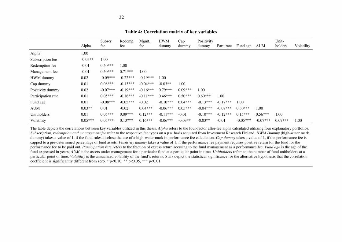
32
Table 4: Correlation matrix of key variables
Alpha Subscr. fee
Redemp. fee
Mgmt. fee
HWM dummy
Cap dummy
Positivity dummy Part. rate Fund age AUM
Unit-holders Volatility
Alpha 1.00
Subscription fee -0.03** 1.00
Redemption fee -0.01 0.50*** 1.00
Management fee -0.01 0.50*** 0.71*** 1.00
HWM dummy 0.02 -0.09*** -0.22*** -0.19*** 1.00
Cap dummy 0.01 0.08*** -0.13*** -0.04*** -0.03** 1.00
Positivity dummy 0.02 -0.07*** -0.19*** -0.16*** 0.79*** 0.09*** 1.00
Participation rate 0.01 0.05*** -0.16*** -0.11*** 0.46*** 0.50*** 0.60*** 1.00
Fund age 0.01 -0.08*** -0.05*** -0.02 -0.10*** 0.04*** -0.13*** -0.17*** 1.00
AUM 0.03** 0.01 -0.02 0.04*** -0.06*** 0.05*** -0.04*** -0.07*** 0.30*** 1.00
Unitholders 0.01 0.05*** 0.09*** 0.12*** -0.11*** -0.01 -0.10*** -0.12*** 0.15*** 0.56*** 1.00
Volatility 0.05*** 0.05*** 0.13*** 0.16*** -0.06*** -0.03** -0.03** -0.01 -0.05*** -0.07*** 0.07*** 1.00
The table depicts the correlations between key variables utilized in this thesis. Alpha refers to the four-factor after-fee alpha calculated utilizing four explanatory portfolios. Subscription, redemption and management fee refer to the respective fee types on a p.a. basis acquired from Investment Research Finland. HWM Dummy (high-water mark dummy) takes a value of 1, if the fund rules disclose the use of a high-water mark in performance fee calculation. Cap dummy takes a value of 1, if the performance fee is capped to a pre-determined percentage of fund assets. Positivity dummy takes a value of 1, if the performance fee payment requires positive return for the fund for the performance fee to be paid out. Participation rate refers to the fraction of excess return accruing to the fund management as a performance fee. Fund age is the age of the fund expressed in years; AUM is the assets under management for a particular fund at a particular point in time. Unitholders refers to the number of fund unitholders at a particular point of time. Volatility is the annualized volatility of the fund’s returns. Stars depict the statistical significance for the alternative hypothesis that the correlation coefficient is significantly different from zero. * p<0.10, ** p<0.05, *** p<0.01

33
5.2. Performance fees in Finnish mutual funds
Overall, based on the sample, the use of performance fees is not very common in Finnish
mutual funds. Only 10.2% of my total observations included the use of performance fees. At
the end of the sample period in December 2012, 12.03% of funds in the sample utilized
performance fees. Summary of the characteristics of performance fees is provided in Table 5
on the next page.
However, contrasting Finland to the Nordic countries9, the use of performance fees is notably
more frequent in Finland than in rest of Nordic countries. At the end of 2012, there were 10
funds in Sweden, 2 funds in Denmark and 38 funds in Norway using performance fees.
Furthermore, the use of performance fees in Finland seems to be more prevalent compared to
the United States, where, according to Elton et al. (2003) only 108 out of a total of 6716 funds
used incentive fees in 1999.
The AUM of funds with performance fees is also smaller. The mean AUM over the sample
for funds with performance fees was €59.3m, whereas for funds without performance fees the
mean AUM was €79.5m. At the end of the sample period, the average AUM for funds with
performance fees was smaller than for funds without performance fees, at €72.2m and
€95.1m, respectively. This is potentially explained by the fact that a majority of funds with
performance fees are managed by firms with lower brand awareness (such as PYN or ODIN),
compared to larger Finnish financial institutions (e.g. Nordea and Pohjola) leading to a
relatively lower AUM. Funds utilizing performance fees in my sample are listed in Appendix
B.
9 My original data request from Morningstar contained also Norwegian, Swedish and Danish mutual funds. This data is to the best extent of my knowledge exhaustive, but has not been cross-referenced against data from other sources and thus is not as reliable as the Finnish data. These funds were dropped from the final study due to country-specific reasons; Norway due to regulatory restrictions on asymmetric fees, Denmark due to very infrequent use of performance fees and the subsequently small sample size and Sweden due to lack of required data.

34
Table 5: Summary of performance fees charged by mutual funds in the sample
Panel A describes the contractual characteristics of the performance fees charged by the 40 Finnish mutual funds in my sample. Participation rate refers to the portion of excess return accruing to management. High-water mark refers to the use of a high-water mark provision in the contract. Positivity constraint limits the payment of performance fees only to cases where the absolute return of a fund is positive. Cap on performance fee limits the performance fee to a predetermined maximum percentage of AUM.
Panel B describes the different types of hurdle rates utilized in the calculation of the performance fees in the funds in my sample. Single market index refers to the use of a single equity or stock index which is used as the reference rate. Combination of multiple indices refers to the combination of multiple indices to a single hurdle rate via taking arithmetic or a weighted average of the underlying indices' returns. Risk-free rate refers to the use of a risk-free rate (in this context, the Euribor rate as well as the TyEl, the Finnish pension rate, have been categorized to be risk-free rates). Fixed rate is a pre-determined fixed return number that must be beat in order for the performance fee to start accruing. No hurdle rate is simply a case, where the fund only needs a positive return for the performance fee to start accruing.
Panel C describes the relationship between the contractual constraints utilized by a fund and the selected hurdle rate. Note that the sums are different from the Panel B due to the fact that a fund may contain several constraints (i.e. a positivity constraint and a high-watermark dummy), whereas the utilized hurdle rates can only be assigned to one of the pre-determined categories.
Panel A: Funds with performance fees and their characteristics
N Mean Max Min St. Dev.
Participation rate 40 16.70 % 30 % 10 % 5.00 % High-water mark 17
(43.3%) Positivity constraint 17
(43.3%)
Panel B: Utilized hurdle rates
Single index Past return Risk-free
rate Fixed rate No rate Multiple
indices
Number of funds 27 1 4 5 2 1 Percentage of total 67.5 % 2.5 % 10.0 % 12.5 % 5.0 % 2.5 %
Panel C: Relationship between characteristics and hurdle rate
Single index Past return Risk-free
rate Fixed rate No hurdle
rate Multiple
indices
High-water mark 4 0 4 5 2 1 Capped fee 4 1 0 0 0 0 Positivity constraint 8 0 4 5 2 0 No constraints 15 0 0 0 0 0
Majority of the funds (67.5%) are using single index as the hurdle rate. Furthermore, the use
of high-water marks is fairly common in fairly frequent in cases, where the hurdle rate is not a
single index. Of the total of 17 funds using a high-water mark, 12 have hurdle rate which is
different from a single index. Perhaps the most interesting data point of the performance fees,
the participation rate is heavily focused at the 20% mark. As is evident in Figure 1, over half
(23) of the 40 funds with performance fees charge a participation rate of 20%.
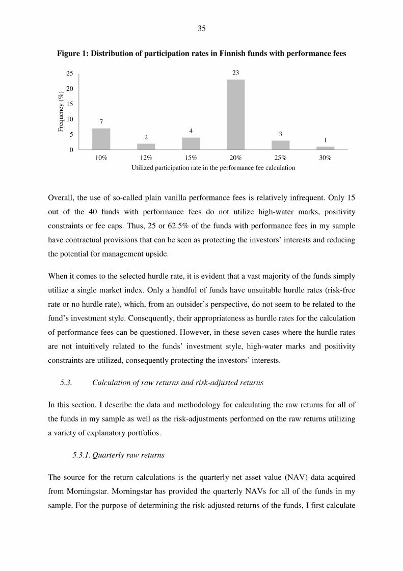
35
Figure 1: Distribution of participation rates in Finnish funds with performance fees
Overall, the use of so-called plain vanilla performance fees is relatively infrequent. Only 15
out of the 40 funds with performance fees do not utilize high-water marks, positivity
constraints or fee caps. Thus, 25 or 62.5% of the funds with performance fees in my sample
have contractual provisions that can be seen as protecting the investors’ interests and reducing
the potential for management upside.
When it comes to the selected hurdle rate, it is evident that a vast majority of the funds simply
utilize a single market index. Only a handful of funds have unsuitable hurdle rates (risk-free
rate or no hurdle rate), which, from an outsider’s perspective, do not seem to be related to the
fund’s investment style. Consequently, their appropriateness as hurdle rates for the calculation
of performance fees can be questioned. However, in these seven cases where the hurdle rates
are not intuitively related to the funds’ investment style, high-water marks and positivity
constraints are utilized, consequently protecting the investors’ interests.
5.3. Calculation of raw returns and risk-adjusted returns
In this section, I describe the data and methodology for calculating the raw returns for all of
the funds in my sample as well as the risk-adjustments performed on the raw returns utilizing
a variety of explanatory portfolios.
5.3.1. Quarterly raw returns
The source for the return calculations is the quarterly net asset value (NAV) data acquired
from Morningstar. Morningstar has provided the quarterly NAVs for all of the funds in my
sample. For the purpose of determining the risk-adjusted returns of the funds, I first calculate
7
24
23
31
0
5
10
15
20
25
10% 12% 15% 20% 25% 30%
Fre
quen
cy (
%)
Utilized participation rate in the performance fee calculation

36
the raw quarterly returns of all the funds in my sample. The NAVs are reported net of fees, so
the calculated returns are net returns. These net returns are subsequently used in the
calculation of risk-adjusted returns.
������,�,� = � �������,� �������,�� − 1
(1)
The returns are calculated on a discrete basis instead of continuous compounding due to the
fact that the returns for the explanatory portfolios used in the risk-adjustment are also
expressed on a discrete basis.
5.3.2. Categorization of funds for calculation of risk-adjusted returns
In order to study the impact of performance fees on funds’ returns, a risk-adjustment to the
calculated raw returns is required, as the differences in returns are partly attributable to
inherent differences in investment styles of the funds. In order to achieve this, I categorize all
of the funds in my sample to five different geographical categories. This is done in order to
strip out the differences in returns caused by different investment styles. The funds are
categorized into the following geographical categories: Europe, Global, Japan, APAC and
North America.
In order to implement the categorization, I looked at the Morningstar category and the
prospectus-defined investment strategy of the fund and grouped the fund into one of the
aforementioned categories. All sector-focused funds (i.e. energy or healthcare) were
categorized into the Global portfolio as well as funds focusing on emerging markets outside
Asia. All Asia-focused funds, regardless of country or investment focus, were included in the
APAC category, apart from Japan.
5.3.3. Explanatory portfolios used for risk-adjustment
Having performed the grouping of the sample funds into the five geographical categories, I
acquire the return data for the explanatory portfolios for calculating the risk-adjusted returns.
The return data for the explanatory portfolios is acquired from scholar Kenneth French’s
website, which is widely used in the calculation of risk-adjusted returns of investments. The
raw data is on a monthly basis and has been converted to quarterly basis to make it
comparable to the data acquired from Morningstar.

37
In order to determine a fund’s risk adjusted return, I have utilized four distinct explanatory
portfolios denoted by Market, SMB, HML and WML, which refer to the market portfolio,
size portfolio, value portfolio and momentum portfolio, respectively. These four factors have
been used in previous literature for calculating the risk-adjusted returns of mutual funds (see
e.g. Carhart, 1997)
The market portfolio refers to a region’s value-weighted market portfolio’s return in excess
over the 1-month Treasury rate.
The SMB or the size portfolio refers to a portfolio mimicking the size anomaly or that small-
cap companies outperform large-cap companies. According to Kenneth French’s website, the
SMB portfolio is constructed as follows
SMB is the equal-weight average of the returns on the three small stock portfolios for the region minus the average of the returns on the three big stock portfolios
The HML portfolio is a portfolio mimicking the value phenomenon in which shares with low
Market-to-Book ratios (high Book-to-Market ratios) outperform shares with high Market-to-
Book ratios (low Book-to-market ratios). The HML portfolio is constructed as follows:
HML is the equal-weight average of the returns for the two high B/M portfolios for a region minus the average of the returns for the two low B/M portfolios
The WML portfolio mimicks the momentum phenomenon, in which stock returns exhibit
positive autocorrelation (i.e. positive stock returns tend to be followed by positive returns and
vice versa). The WML portfolio is constructed as follows
WML is the equal-weight average of the returns for the two winner portfolios for a region minus the average of the returns for the two loser portfolios
Overview of the returns of the explanatory portfolios is depicted in Appendix C.
5.3.4. Calculation of risk-adjusted returns
Having acquired the quarterly raw returns for the funds and the quarterly returns of the
explanatory portfolios, I am able to calculate the quarterly risk-adjusted return (henceforth
also referred to as the “four-factor alpha”, “ex-post alpha”, “Jensen’s alpha” or simply
“alpha”) for each of the observations in my sample. To do this, I utilize the 4-factor model
originally introduced by Carhart (1997). The model includes the traditional three Fama-

38
French risk factors (market, size and value) and an additional factor capturing the momentum
anomaly.
The risk-adjusted performance is estimated separately based on geographic categorization g
for each fund i at time t using the following equation,
�����,�,� − ��,�,�,� = �����,� + ��(�������,�,�,� − ��,�,�,�) + � �!�",�,�,� +�#�$�%,�,�,� + �&��'(����(,,�,�,�
(2)
where �����,�,� − ��,�,�,� is the fund’s net return for period )* to )� in excess of the risk-
free rate.�������,�,�,� − ��,�,�,� is the return of the market portfolio in excess of the same
risk-free rate. �!�",�,�,�and �$�%,�,�,� are returns on portfolios mimicking Fama-French
factors size and book-to-market equity. ��'(����(,,�,�,� is the return of the portfolio
mimicking the momentum strategy.10
By estimating the equation I obtain the beta coefficients for each of the factors for each fund
in the sample. Utilizing the estimated beta coefficients for the sample period, I acquire the
theoretical model return for the each time period for each fund in the sample. By comparing
the model return and the realized return for the time period, I obtain the funds’ ex post four-
factor alpha (“Jensen’s alpha”), which is a risk-adjusted return measure for all of the funds in
the sample taking into account the differences in investment focus. A summary of the alphas
is depicted in Table 6 below.
10 The data for the three Fama-French factors has been acquired from Kenneth French’s website http://mba.tuck.dartmouth.edu/pages/faculty/ken.french/data_library.html.

39
Table 6: Estimated quarterly ex post four-factor alphas of the funds in the sample
Category N Mean St. Dev. Min Max
APAC 494 1.02E-08 8.39 % -22.93 % 34.32 %
Europe 3019 4.01E-08 7.75 % -56.03 % 56.26 %
Global 1688 -9.84E-10 6.40 % -25.20 % 30.11 %
Japan 148 9.46E-09 4.96 % -14.29 % 11.59 %
NorthAmerica 298 2.55E-08 4.84 % -12.89 % 17.96 %
Total 5647 2.36E-08 7.24 % -56.03 % 56.26 %
This table summarizes the estimated four-factor alphas (risk-adjusted returns) for each of the funds in the sample across time estimated using equation 12. The explanatory portfolios used in the calculation of alphas are market portfolio (RMRF), size portfolio (SMB), value portfolio (HML) and momentum portfolio (WML).
On average, the funds are unable to provide superior risk-adjusted returns, which is evident in
the average alphas, which are very close to zero. The estimated minimum and maximum ex-
post alphas are rather large in absolute terms, which is to be expected due to the sample size.
5.4. Tracking error data and calculations
In order to calculate the tracking error of fund returns and correlation between the fund and
the benchmark, I obtain additional data. As the data from Morningstar or Investment Research
Finland did not include data on tracking errors or correlations, I acquired the data for these
calculations via the Bloomberg portal, using the ISIN codes of the funds in my sample. For
acquiring the benchmark return data, I matched the benchmark stated in the Morningstar
data/IRF data/Fund prospectus to a specific Bloomberg ticker using Bloomberg’s search
functionality. After having all the ticker codes for the funds and benchmarks, I acquired net
asset value on a monthly basis for the time period of 2007-2012. Having acquired the absolute
ending values, I calculated the monthly returns for the fund and benchmark11 in question. The
acquisition of return data for the funds is done for the second time to ensure that the utilized
time period is exactly the same for the fund and the benchmark.
Unfortunately, for some of the funds, benchmark was not disclosed or utilized at all.
Consequently, funds without a benchmark were dropped from the calculations. Moreover, for
some of the benchmarks, the benchmark price data was not available from Bloomberg, which
forced me to drop funds utilizing such benchmarks from the calculations. For the
aforementioned reasons, I ended up with 238 funds, where I had return data for both the fund
11 Some of the funds utilized a weighted average of several benchmarks’ returns. In these cases, I simply acquired the ending prices for each of the components, calculated the return for each of the component and utilized the prospectus-stated weights to calculate the benchmark return. For instance, the fund Eufex ActiveAlpha has a benchmark consisting of three components: MSCI AC Americas NR USD 33.000% + MSCI AC Asia NR USD 33.000% + MSCI AC Europe NR USD 34.000%

40
and the benchmark for a given time period. This is considerably smaller than my original
sample of 332 funds. Having calculated the returns for the funds and the benchmarks, I
calculated the annualized tracking error for the funds in the sample utilizing the following
formula.
,-./01234--5-6. .. = √12 ∗ ;<=�����,�,� − �"��>?(���,�,�@ , − 1A�B* (3)
An overview of the descriptive statistics between the total sample and for the subsample on
which the tracking error calculations are performed is available in Appendix D. Overall, the
funds for which benchmark data was available are larger in terms of AUM, slightly older and
have more unitholders. These funds can thus be characterized as being more established as
they have a longer track record and more owners. The funds with no benchmark data
available are newer and have less unitholders.

41
6. Analysis and results
The following analysis section is divided into four discrete parts. First, in part 6.1 I study the
impact of the use of performance fees on mutual funds’ risk-adjusted returns as measured by
the fund’s four-factor alpha and Sharpe ratio. Next, in section 6.2, I study the impact of
performance fees on fund managers’ risk-taking behaviour as measured by fund volatility and
tracking errors. In section 6.3 I present my methodology for calculating the ex ante value of
the performance fees and results of the valuation. Following the calculation of the cost of the
fees, I compare the costs of funds with performance fees to funds without such fees in part
6.4.
6.1. Performance fees and fund returns
In order to answer my first research question on the relationship between performance fees
and fund returns, I conduct a variety of regressions to test the relationship between
performance fees and returns, utilizing a variety of return measures.
In the following chapters, I present my methodology and analysis for determining the impact
of performance fees on the mutual funds’ raw and risk-adjusted returns. The regression
equations in this section utilize a variety of return measures, including raw, non-adjusted
quarterly returns, quarterly four-factor alphas (as calculated in part 5.3.4) and annual Sharpe
ratios. The equations follow the work of Massa and Patgiri (2009) and Elton et al. (2003),
with some modifications partly due to differences in research focus and partly due to data
availability reasons. The key difference between my work and that of Massa and Patgiri
(2009) is the inclusion of performance fee dummy as an explanatory variable and the
omission of fund survival probability and turnover ratio due to data reasons.
Furthermore, to control for fund-specific characteristics, I include a variety of control
variables related to fund size and age in the regression specifications.
6.1.1. Impact of performance fees on funds’ raw, non-risk-adjusted returns
To determine the impact of the use of performance fees on the raw quarterly returns of mutual
funds as calculated in part 5.3.1, I estimate the following equation,
������,�,� = �* + ��CD + � ED + F����,� (4)
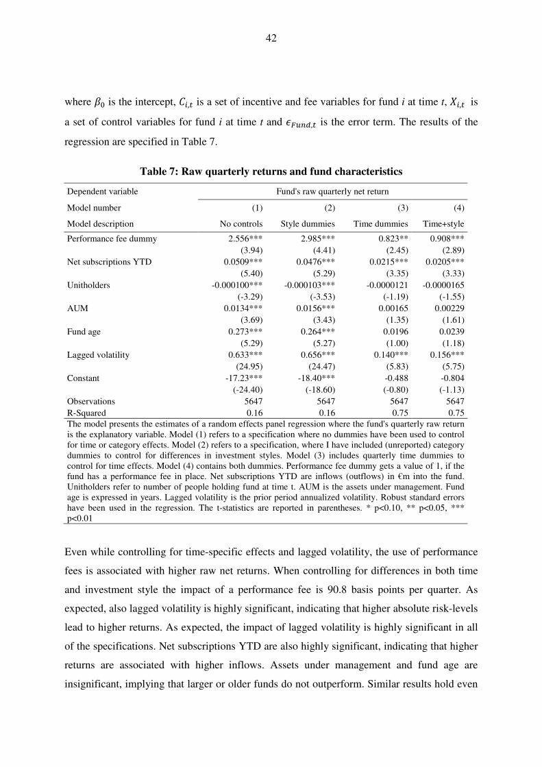
42
where �* is the intercept, CD,� is a set of incentive and fee variables for fund i at time t, ED,� is
a set of control variables for fund i at time t and F����,� is the error term. The results of the
regression are specified in Table 7.
Table 7: Raw quarterly returns and fund characteristics
Dependent variable Fund's raw quarterly net return
Model number (1) (2) (3) (4)
Model description No controls Style dummies Time dummies Time+style
Performance fee dummy 2.556*** 2.985*** 0.823** 0.908***
(3.94) (4.41) (2.45) (2.89)
Net subscriptions YTD 0.0509*** 0.0476*** 0.0215*** 0.0205***
(5.40) (5.29) (3.35) (3.33)
Unitholders -0.000100*** -0.000103*** -0.0000121 -0.0000165
(-3.29) (-3.53) (-1.19) (-1.55)
AUM 0.0134*** 0.0156*** 0.00165 0.00229
(3.69) (3.43) (1.35) (1.61)
Fund age 0.273*** 0.264*** 0.0196 0.0239
(5.29) (5.27) (1.00) (1.18)
Lagged volatility 0.633*** 0.656*** 0.140*** 0.156***
(24.95) (24.47) (5.83) (5.75)
Constant -17.23*** -18.40*** -0.488 -0.804
(-24.40) (-18.60) (-0.80) (-1.13)
Observations 5647 5647 5647 5647
R-Squared 0.16 0.16 0.75 0.75
The model presents the estimates of a random effects panel regression where the fund's quarterly raw return is the explanatory variable. Model (1) refers to a specification where no dummies have been used to control for time or category effects. Model (2) refers to a specification, where I have included (unreported) category dummies to control for differences in investment styles. Model (3) includes quarterly time dummies to control for time effects. Model (4) contains both dummies. Performance fee dummy gets a value of 1, if the fund has a performance fee in place. Net subscriptions YTD are inflows (outflows) in €m into the fund. Unitholders refer to number of people holding fund at time t. AUM is the assets under management. Fund age is expressed in years. Lagged volatility is the prior period annualized volatility. Robust standard errors have been used in the regression. The t-statistics are reported in parentheses. * p<0.10, ** p<0.05, *** p<0.01
Even while controlling for time-specific effects and lagged volatility, the use of performance
fees is associated with higher raw net returns. When controlling for differences in both time
and investment style the impact of a performance fee is 90.8 basis points per quarter. As
expected, also lagged volatility is highly significant, indicating that higher absolute risk-levels
lead to higher returns. As expected, the impact of lagged volatility is highly significant in all
of the specifications. Net subscriptions YTD are also highly significant, indicating that higher
returns are associated with higher inflows. Assets under management and fund age are
insignificant, implying that larger or older funds do not outperform. Similar results hold even
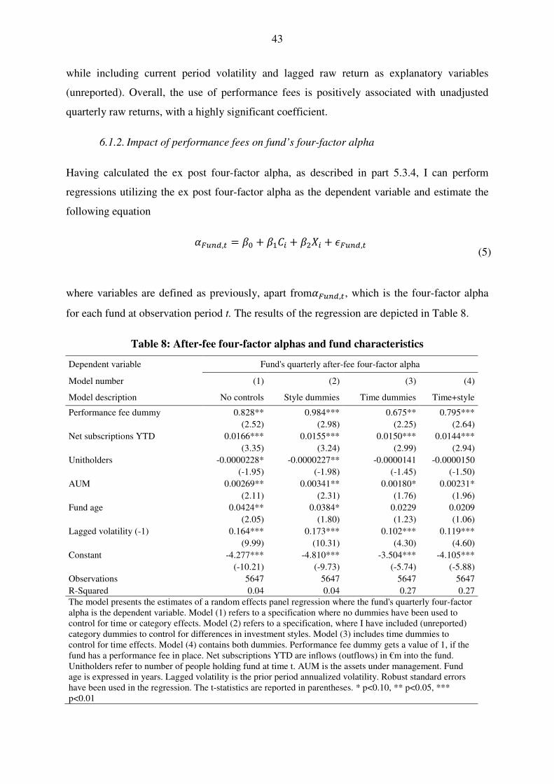
43
while including current period volatility and lagged raw return as explanatory variables
(unreported). Overall, the use of performance fees is positively associated with unadjusted
quarterly raw returns, with a highly significant coefficient.
6.1.2. Impact of performance fees on fund’s four-factor alpha
Having calculated the ex post four-factor alpha, as described in part 5.3.4, I can perform
regressions utilizing the ex post four-factor alpha as the dependent variable and estimate the
following equation
�����,� = �* + ��CD + � ED + F����,�
(5)
where variables are defined as previously, apart from�����,�, which is the four-factor alpha
for each fund at observation period t. The results of the regression are depicted in Table 8.
Table 8: After-fee four-factor alphas and fund characteristics
Dependent variable Fund's quarterly after-fee four-factor alpha
Model number (1) (2) (3) (4)
Model description No controls Style dummies Time dummies Time+style
Performance fee dummy 0.828** 0.984*** 0.675** 0.795***
(2.52) (2.98) (2.25) (2.64)
Net subscriptions YTD 0.0166*** 0.0155*** 0.0150*** 0.0144***
(3.35) (3.24) (2.99) (2.94)
Unitholders -0.0000228* -0.0000227** -0.0000141 -0.0000150
(-1.95) (-1.98) (-1.45) (-1.50)
AUM 0.00269** 0.00341** 0.00180* 0.00231*
(2.11) (2.31) (1.76) (1.96)
Fund age 0.0424** 0.0384* 0.0229 0.0209
(2.05) (1.80) (1.23) (1.06)
Lagged volatility (-1) 0.164*** 0.173*** 0.102*** 0.119***
(9.99) (10.31) (4.30) (4.60)
Constant -4.277*** -4.810*** -3.504*** -4.105***
(-10.21) (-9.73) (-5.74) (-5.88)
Observations 5647 5647 5647 5647
R-Squared 0.04 0.04 0.27 0.27
The model presents the estimates of a random effects panel regression where the fund's quarterly four-factor alpha is the dependent variable. Model (1) refers to a specification where no dummies have been used to control for time or category effects. Model (2) refers to a specification, where I have included (unreported) category dummies to control for differences in investment styles. Model (3) includes time dummies to control for time effects. Model (4) contains both dummies. Performance fee dummy gets a value of 1, if the fund has a performance fee in place. Net subscriptions YTD are inflows (outflows) in €m into the fund. Unitholders refer to number of people holding fund at time t. AUM is the assets under management. Fund age is expressed in years. Lagged volatility is the prior period annualized volatility. Robust standard errors have been used in the regression. The t-statistics are reported in parentheses. * p<0.10, ** p<0.05, *** p<0.01
44
Despite the risk-adjustment made based on inherent differences in funds’ investment styles,
the impact of performance fees on risk-adjusted returns is similar as their impact on raw
returns. Performance fee dummy is highly significant and is associated with a 79.5 basis point
increase in quarterly alpha. These findings are also in line with Massa and Patgiri (2009), who
find that higher contractual incentives increase risk-adjusted returns. Furthermore,
Ackermann et al. (2002) find that incentive fees have a strong positive impact on risk-
adjusted return. Thus, overall, my results are in line with the (scarce) existing literature,
giving support to my first hypothesis that higher contractual incentives are associated with
superior performance.
The magnitude of the impact of the incentives is also roughly in line with previous literature.
My finding of excess return of 79.5 basis points per quarter (or 318 basis points p.a.) is in line
with Massa and Patgiri (2009), who, albeit using a slightly different methodology, find that
top-incentive quintile outperforms the bottom quintile by 2.70% p.a. Furthermore, Golec
(1988) finds that funds with incentive fees exhibit on average 1.62% higher alphas on an
annual basis.
Fund age does not have any impact on a fund’s risk-adjusted return. In other words, older or
younger funds do not vary in terms of their return-producing capabilities. This observation is
in contrast with the study of Massa and Patgiri (2009), who find a significant relationship
between fund age and risk-adjusted returns. However, the absolute magnitude of their
coefficient, despite its statistical significance, is rather small. However, in the study of
Ackermann et al. (2002), fund age never significantly impacts a fund’s return. My
observations are in line with these findings.
Overall, my results imply a positive association between the use of performance fees and ex
post alpha, even while controlling for time-specific factors and fund volatility.
6.1.3. Impact of performance fees on a fund’s Sharpe ratio
To control for any possible inappropriate categorisations in part 5.3.2 and consequently
inaccurate risk-adjusted alphas, I also utilize the Sharpe ratio as a measure of risk-adjusted
performance. By utilizing the Sharpe ratio as a measure of risk-adjusted performance, I am
able to avoid any assumptions about appropriate explanatory portfolios for the funds in the
sample. The Sharpe ratio has been directly acquired from IRF data and it is stated on a yearly
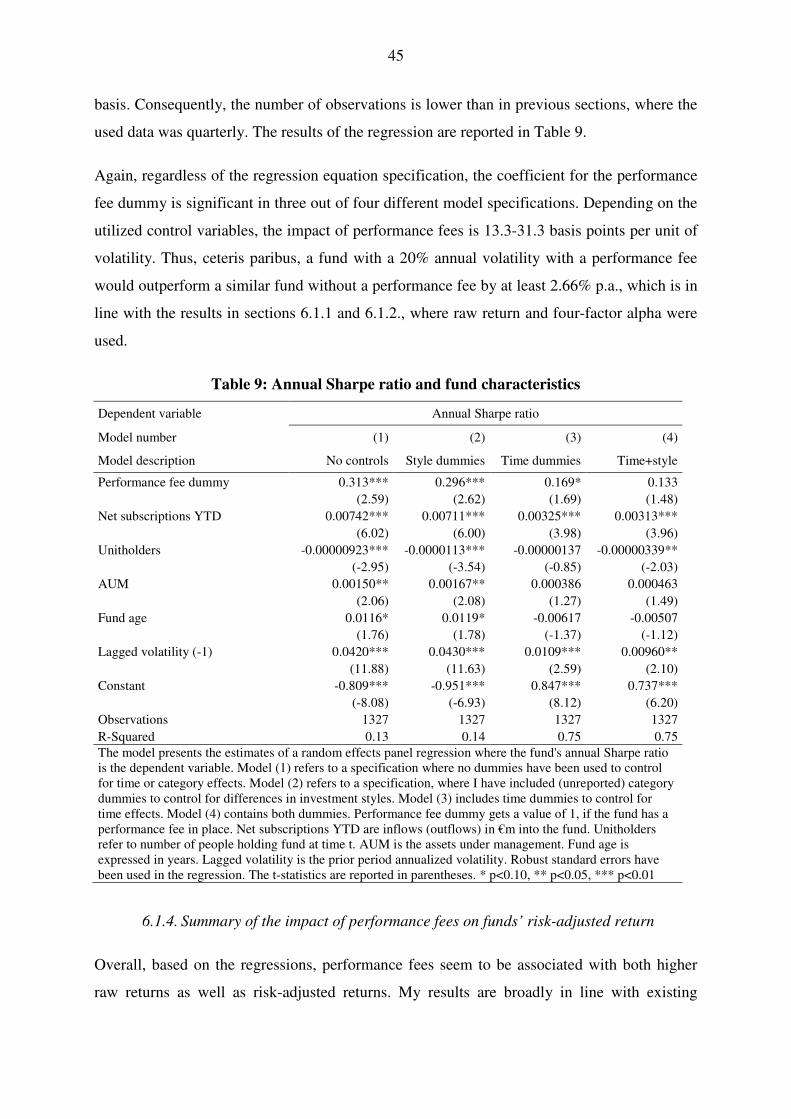
45
basis. Consequently, the number of observations is lower than in previous sections, where the
used data was quarterly. The results of the regression are reported in Table 9.
Again, regardless of the regression equation specification, the coefficient for the performance
fee dummy is significant in three out of four different model specifications. Depending on the
utilized control variables, the impact of performance fees is 13.3-31.3 basis points per unit of
volatility. Thus, ceteris paribus, a fund with a 20% annual volatility with a performance fee
would outperform a similar fund without a performance fee by at least 2.66% p.a., which is in
line with the results in sections 6.1.1 and 6.1.2., where raw return and four-factor alpha were
used.
Table 9: Annual Sharpe ratio and fund characteristics
Dependent variable Annual Sharpe ratio
Model number (1) (2) (3) (4)
Model description No controls Style dummies Time dummies Time+style
Performance fee dummy 0.313*** 0.296*** 0.169* 0.133
(2.59) (2.62) (1.69) (1.48)
Net subscriptions YTD 0.00742*** 0.00711*** 0.00325*** 0.00313***
(6.02) (6.00) (3.98) (3.96)
Unitholders -0.00000923*** -0.0000113*** -0.00000137 -0.00000339**
(-2.95) (-3.54) (-0.85) (-2.03)
AUM 0.00150** 0.00167** 0.000386 0.000463
(2.06) (2.08) (1.27) (1.49)
Fund age 0.0116* 0.0119* -0.00617 -0.00507
(1.76) (1.78) (-1.37) (-1.12)
Lagged volatility (-1) 0.0420*** 0.0430*** 0.0109*** 0.00960**
(11.88) (11.63) (2.59) (2.10)
Constant -0.809*** -0.951*** 0.847*** 0.737***
(-8.08) (-6.93) (8.12) (6.20)
Observations 1327 1327 1327 1327
R-Squared 0.13 0.14 0.75 0.75
The model presents the estimates of a random effects panel regression where the fund's annual Sharpe ratio is the dependent variable. Model (1) refers to a specification where no dummies have been used to control for time or category effects. Model (2) refers to a specification, where I have included (unreported) category dummies to control for differences in investment styles. Model (3) includes time dummies to control for time effects. Model (4) contains both dummies. Performance fee dummy gets a value of 1, if the fund has a performance fee in place. Net subscriptions YTD are inflows (outflows) in €m into the fund. Unitholders refer to number of people holding fund at time t. AUM is the assets under management. Fund age is expressed in years. Lagged volatility is the prior period annualized volatility. Robust standard errors have been used in the regression. The t-statistics are reported in parentheses. * p<0.10, ** p<0.05, *** p<0.01
6.1.4. Summary of the impact of performance fees on funds’ risk-adjusted return
Overall, based on the regressions, performance fees seem to be associated with both higher
raw returns as well as risk-adjusted returns. My results are broadly in line with existing

46
research (see Agarwal et al., 2009; Elton et al., 2003; Golec, 1988 and Massa and Patgiri,
2009) which suggests that higher contractual incentives are associated with better
performance.
The results are robust across different model specifications and different dependent variables,
which increases the confidence in my results. Out of a total of 12 models (4 different
specifications with 3 different dependent variables), the coefficient for the performance fee
dummy is significant in eleven cases. As expected, lagged volatility has a significant impact
on the performance of a fund due to the positive relationship between risk and expected
return.
6.2. Performance fees and fund management behaviour
As discussed, performance fees are effectively a spread option held by the management and
written by the investors on the excess return of the fund. The spread option increases in value
when either the volatility of the fund increases or the correlation between the fund returns and
the benchmark returns decreases. In line with my second research question, in this section I
study the impact of performance fees on a variety of risk-measures to determine whether the
use of performance fees is associated with higher absolute and/or active risk.
Due to the option-like nature of the performance compensation, funds with performance fees
theoretically have a larger incentive to take risk. As Drago et al. (2005) and Margrabe (1978)
note, the volatility of a spread option is defined as
GH = IG� − 2J�, G�G + G (6)
As the vega, or the first derivative of option value with regards to volatility, of the long spread
option is positive, increasing the volatility GH of the spread option will increase the value of
the option. This can be achieved either via increasing the absolute volatility of the fund
portfolio (G� ) by for example increasing leverage or decreasing the correlation with the
benchmark (J�, ). Both of these actions will increase the deviation of the fund’s returns
around the benchmark and consequently increase the probability of the performance fee
option ending in the money. Thus, based on the aforementioned reasoning, I test statistically
both whether funds with performance fees exhibit absolute higher risk levels (i.e. is G� on

47
average higher) and whether such funds exhibit higher active risk levels (i.e. is the tracking
error of the fund higher)
6.2.1. Performance fees and volatility levels
With regards to the absolute risk levels, I estimate the impact of contractual incentives on the
absolute risk of a fund by the equation
GD,� = �* + �*CD,� + ��ED,� + FD,� (7)
where GD,� is the annualized volatility of returns for fund i at time t, CD,� is a dummy for the use
of performance fee and ED,� is a set of control variables. As previously, my specification is for
most part following the methodology of Massa and Patgiri (2009) with the difference that I
am using a performance fee dummy as an explanatory variable instead of the Coles’ incentive
rate.
The model specification for the regressions is similar as in part 6.1. However, in this section, I
have also included fees (subscription, redemption, management) as explanatory variables to
test for the impact of fees on the volatility of funds in the sample. These were excluded from
the return regressions due to the fact that all used return measures were based on after-fee
returns. Consequently, including the fees in the return regressions would have had no
economic interpretation.
The results of the regression, depicted in Table 10, are surprising. In the first two model
specifications, the impact of performance fee on volatility is negative. However, when
controlling for time effects, which often have a significant impact on volatility, the effect of
performance fees on volatility is not significant. As expected, the volatility of the previous
period has quite a large impact on the volatility of the subsequent period. Interestingly, fund
age has a positive impact on volatility, implying that older funds take slightly higher risk,
when controlling for time effects. The R-squared for the models is relatively large due to the
inclusion of lagged volatility and time dummies, which explain most of the variation in
volatility. Thus, based on the empirical findings, funds with performance fees do not seem to
exhibit higher absolute risk levels compared to their peers. The empirical evidence does not
support the hypothesis that funds with performance fees take higher risk than normal funds.

48
The insignificance of the performance fee dummy is in contrast to the study of Massa and
Patgiri (2009), who find that higher contractual incentives are associated with higher risk-
taking, albeit using a different definition of incentives. However, my results are in line with
the findings of Gehrig et al. (2008), who find, albeit using a survey-based methodology, that
there is little evidence of bonus payments inducing risk-taking. With respect to the theoretical
literature, my empirical results provide support to Carpenter (2000) who finds that option-like
compensation does not lead to strictly higher risk seeking.
Interestingly, the coefficient for unitholders is highly significant, implying that funds with a
larger number of subscribers have larger volatility levels. However, the coefficient for AUM
is negative and significant, implying that an increase in AUM would result in a decrease in
volatility. Fund age has a marginal but significant impact on volatility, implying that older
funds are taking more absolute risk.

49
Table 10: Use of performance fees and mutual fund volatility
Dependent variable Fund i's annualized quarterly volatility at time t
Model number (1) (2) (3) (4)
Model description No controls Style dummies Time dummies Time+style
Performance fee dummy -0.431** -0.538*** 0.141 0.0852
(-2.30) (-2.72) (1.45) (0.90)
Subscription fee 0.123 0.162 -0.0499 -0.0393
(0.73) (0.89) (-0.67) (-0.48)
Redemption fee -0.198 -0.114 -0.0671 -0.0175
(-1.09) (-0.59) (-0.83) (-0.20)
Management fee 0.249** 0.154 0.165*** 0.119**
(2.12) (1.27) (3.21) (2.27)
Net subscriptions YTD -0.0161*** -0.0152*** -0.00612*** -0.00581***
(-6.06) (-5.62) (-3.69) (-3.42)
Unitholders 0.0000216** 0.0000227*** 0.0000165*** 0.0000177***
(2.48) (2.61) (2.93) (3.02)
AUM -0.00304*** -0.00358*** -0.00319*** -0.00348***
(-2.68) (-2.58) (-3.20) (-2.98)
Fund age -0.0617*** -0.0592*** 0.0217*** 0.0219***
(-4.28) (-4.25) (2.79) (2.86)
Lagged volatility 0.850*** 0.844*** 0.944*** 0.937***
(144.72) (137.10) (134.20) (121.91)
Constant 3.776*** 4.290*** -0.922*** -0.528**
(15.19) (13.75) (-5.02) (-2.50)
Observations 4842 4842 4842 4842
R-squared 0.74 0.75 0.81 0.81
This table describes the results of a regression of a mutual fund's annualized volatility at time t on a set of explanatory variables. The t-statistics are reported in parentheses. Robust standard errors have been used to correct for heteroskedasticity. Model (1) refers to a specification where no dummies have been used to control for time or category effects. Model (2) refers to a specification, where I have included (unreported) category dummies to control for differences in investment styles. Model (3) includes time dummies to control for time effects. Model (4) contains both dummies. . Performance fee dummy gets a value of 1, if the fund has a performance fee in place. Net subscriptions YTD are inflows (outflows) in €m into the fund. Unitholders refer to number of people holding fund at time t. AUM is the assets under management. Fund age is expressed in years. Lagged volatility is the prior period annualized volatility. Robust standard errors have been used in the regression. The t-statistics are reported in parentheses. * p<0.10, ** p<0.05, *** p<0.01
6.2.2. Differences in tracking error
As shown by Chen and Pennacchi (2009), for particular compensation types, a fund manager
will increase the fund’s tracking error as its relative performance declines. In general, a fund
manager under incentive compensation relative to a benchmark will have an incentive to
increase the active risk of her portfolio, i.e. deviate more from the benchmark. This effect is

50
exacerbated when the fund is underperforming the benchmark, as the fund manager will have
incentives to deviate from the benchmark to get back in-the-money in terms of his option
position. The deviation from the benchmark is measured by tracking error, which is the
standard deviation of the difference in returns between the fund and the benchmark:
,-./01234--5- = ;<=�����,� − �"��>?(���,�@ , − 1A�B* (8)
Thus, whereas in part 6.2.1 I test whether performance fees have an impact on the absolute
risk of the fund, in this part I empirically test whether performance fees have an impact on the
active risk of a fund. I empirically test whether there is a difference between the tracking
errors of performance-fee funds and non-performance fee funds.12 The expectation based on
theoretical literature is that funds with performance fees are more aggressive in taking active
risk by deviating from the benchmark more. To test for this, I compare the average tracking
errors for funds with performance fees and without. The results are shown in Table 11.
Table 11: Differences in tracking errors
The table describes the annualized tracking errors for the funds in the sample. The tracking errors are calculated as the standard deviation of the difference in returns of the fund and the benchmark. The data for the calculations has been gathered manually from Bloomberg. To ensure an adequate calculation horizon, the tracking errors have been calculated utilizing differences in returns between March 2007 and December 2012. The lower part of the table describes the results of a statistical test for a significant difference in the mean tracking errors between funds with performance fees and without performance fees.
n Mean St. Dev. Min Max
No performance fee 219 9.55 % 4.58 % 0.00 % 23.85 %
Performance fee 19 13.64 % 8.68 % 4.10 % 39.83 %
Total 238 10.02 % 5.36 % 0.00 % 39.83 %
Difference -4.09 %
Degrees of freedom 236
t-value -3.97
p-value (difference <0) <0.001
Interestingly, based on the results, it seems that funds with performance fees indeed have, on
average, higher tracking errors than funds without performance fees. The results are highly
significant. Contrasting this with my findings in the previous section and previous literature, it
seems that performance fees are associated with higher active risk-taking in the sense that
12 As stated in part 1.4, the tracking error calculations have been done individually for each fund and the corresponding benchmark and are subject to additional data availability restrictions.
51
funds deviate more from their prospectus-stated benchmarks. However, in terms of absolute
risk as measured by the volatility of the funds, funds with performance fees do not take more
risk, which was observed in part 6.2.1.
6.2.3. Summary of performance fees and fund management behaviour
Previous theoretical literature argues that performance fees drive risk-taking, as higher
volatility and/or deviation from the benchmark increases the value of the performance fee
option, albeit in the current period. Moreover, the risk-taking has also been observed
empirically. My results give support to the claim that performance fees are indeed associated
with higher active risk-taking as measured by the tracking error. However, based on my
results, there is no support to the hypothesis mentioned in previous literature that performance
fees drive absolute risk-taking as measured by volatility. The latter finding is potentially
explained by the fact that in my sample and in Finnish mutual funds in general, performance
fees are often associated with contractual mechanisms such as high-water marks that reduce
the incentive for “putting it all on black”. Furthermore, as discussed, an increase in current
period volatility may have an adverse impact on the value of the performance fee in the
subsequent periods and thus.
6.3. Valuation of the performance fee option
In this section, I elaborate on the general principles behind the valuation of the performance
fee option and present the results of my valuation utilizing simulation and the Margrabe
(1978) model for the 40 Finnish mutual funds in my sample charging performance fees.
6.3.1. Introduction to the valuation of the performance fee
As noted by Drago et al. (2005), for a single unit of managed capital, the compensation
payable to the fund management p.a. is
,C = .* ∗ �KL + .�L.M=�����,�,� − �"��>?(���,�,� − N; 0@ ∗ �KL (9)
where TC is total compensation, .* is a factor for management, redemption and subscription
fees, which are usually based on a fixed percentage of AUM, .� is the participation rate, ����� is the return of the fund for the time period from )* to )�, �"��>?(��� is the return
(hurdle rate) for the benchmark for the same period and N is the minimum excess return that
needs to be earned over the hurdle rate before the performance fee starts accruing. Note that in
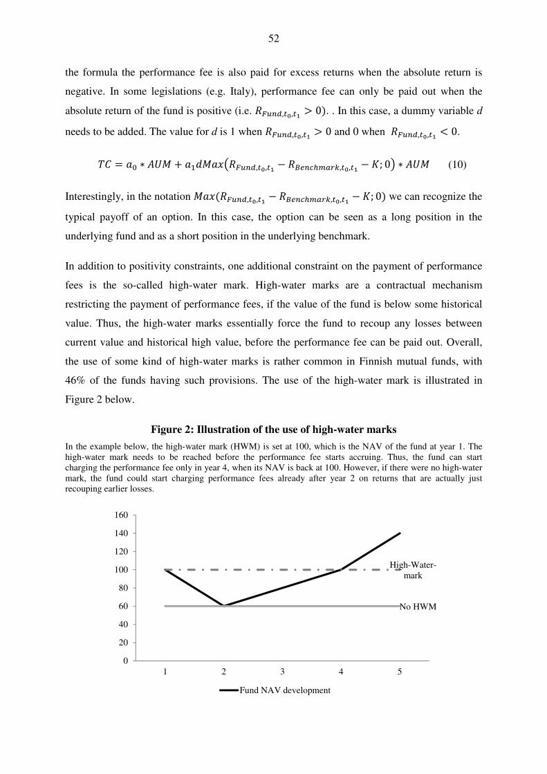
52
the formula the performance fee is also paid for excess returns when the absolute return is
negative. In some legislations (e.g. Italy), performance fee can only be paid out when the
absolute return of the fund is positive (i.e. �����,�,� > 0). . In this case, a dummy variable d
needs to be added. The value for d is 1 when �����,�,� > 0 and 0 when �����,�,� < 0.
,C = .* ∗ �KL + .�SL.M=�����,�,� − �"��>?(���,�,� − N; 0@ ∗ �KL (10)
Interestingly, in the notation L.M(�����,�,� − �"��>?(���,�,� − N; 0) we can recognize the
typical payoff of an option. In this case, the option can be seen as a long position in the
underlying fund and as a short position in the underlying benchmark.
In addition to positivity constraints, one additional constraint on the payment of performance
fees is the so-called high-water mark. High-water marks are a contractual mechanism
restricting the payment of performance fees, if the value of the fund is below some historical
value. Thus, the high-water marks essentially force the fund to recoup any losses between
current value and historical high value, before the performance fee can be paid out. Overall,
the use of some kind of high-water marks is rather common in Finnish mutual funds, with
46% of the funds having such provisions. The use of the high-water mark is illustrated in
Figure 2 below.
Figure 2: Illustration of the use of high-water marks
In the example below, the high-water mark (HWM) is set at 100, which is the NAV of the fund at year 1. The high-water mark needs to be reached before the performance fee starts accruing. Thus, the fund can start charging the performance fee only in year 4, when its NAV is back at 100. However, if there were no high-water mark, the fund could start charging performance fees already after year 2 on returns that are actually just recouping earlier losses.
High-Water-mark
No HWM
0
20
40
60
80
100
120
140
160
1 2 3 4 5
Fund NAV development

53
Expanding the aforementioned notation, total manager compensation with the high-water
mark is
,C = .* ∗ �KL + .�4L.M(�����,�,� − �"��>?(���,�,� − N; 0) (11)
where e is a dummy variable, which gets a value of 1 when NAVWXYZ,[ > NAV\]^ and a
value of 0 when NAVWXYZ,[ < NAV\]^.
Based on equations (9), (10) and (11), there are three main types of performance fee options:
pure, “plain vanilla”, fee; fee with positivity constraint and a fee with a high-water mark. The
benchmark return �"��>?(���,�,� can also consist of a fixed rate instead of the rate of return
on a benchmark portfolio. In some cases, even the risk-free rate (12-month euribor) is used as
the benchmark rate.
Regardless of the details of the performance fee provision, all of the formulas above contain
an option-like compensation component; if the return of the underlying (fund portfolio)
exceeds that of the benchmark, the fund manager is paid a certain fraction of the excess part.
Otherwise the payoff from the option component is zero and the management is compensated
only based on the fixed component .* ∗ �KL.
As discussed in various papers (e.g. Drago et al., 2005; Elton et al., 2003 and Kritzman,
1987), performance fees can be seen as a type of spread option, or the option to exchange one
asset for another. Consequently, option-valuation techniques may be utilized to attempt to
arrive at a monetary value for the performance fee option, albeit with some limitations (see
Drago et al., 2005; Margrabe, 1978 and Wilmott, 2007).
The dollar value of the spread option essentially depends on five factors: (1) the difference
between the standard deviation of the portfolio and the benchmark, (2) the correlation
between the benchmark and the portfolio, (3) the value of assets under management, (4) the
management’s participation rate and (5) the performance measurement period. Interestingly,
via their investment decisions, the management has direct control over the first two factors.
The fund management can increase the difference between the standard deviation of the
portfolio and the benchmark via higher risk-taking by increasing leverage. The management
also has the potential to take more active risk by deviating more from the benchmark,
consequently reducing correlation. As a consequence, a moral hazard dilemma arises: the
management can increase the value of their option via decisions that are not optimal from an

54
investor’s point of view (Kritzman, 1987). This observation is also suggested by Huang et al.
(2011) who note that if fund managers are evaluated on their performance relative to a
benchmark, they are incentivized to increase the standard deviation of the tracking error13.
The payoff of the performance fee with a participation rate of _ to the management in the
most basic case is
L.M=�����,�,� − �"��>?(���,�,� − N; 0@ ∗ �KL ∗ _ (12)
If the strike K (or required excess return over benchmark) is zero, the option can be seen as
option to exchange one asset for another14. Margrabe (1978) provides a valuation formula for
such options, if the strike is zero, even if the two assets are not exchanged in a 1-to-1 ratio.
In a general case for the spread option, where the holder has a right to exchange one asset to
another, in some ratio, the payoff for the contract at expiry is, where
L.M(`�a� − ` a , 0) (13)
`� and` are constants, a� is the price of asset 1 at expiration, a is the price of asset 2 at
expiration.
As introduced originally by Margrabe (1978) and further explained by Wilmott (2007), the
value for such an option is
�(a�, a , )) = `�a�4bc(Ab�) (S�) − ` a 4bcd(Ab�) (S ) (14)
13 There are, however, a few caveats to this argument. As noted by Drago, Lazzari, and Navone (2005), there are indirect effects working in an opposite direction. Firstly, the flow-performance relationship (see e.g. Chevalier and Ellison (1997) means that poorly-performing managers will face outflows, meaning lower assets under management, which will mean a lower dollar management fee. An increase in fund volatility increases the probability of poor performance and thus increases the probability of lower compensation from annual management fees for the manager. Secondly, the above argumentation on tracking error maximization implicitly assumes that managers maximize their single-period wealth. However, in reality (see e.g. (Goldman and Slezak, 2003) portfolio management involves multiple time periods and career concerns of mutual fund managers play a role in portfolio management decisions (Chevalier and Ellison, 1999).Thus, despite the existence of performance fees and the consequent risk-taking incentive, managers also take their future income into account and adjust their risk-taking. Simply put, managers don’t want to get fired and lose their income in subsequent periods. 14 To illustrate the idea behind the exchange option, one may think of the following example. At the beginning of a period, both the mutual fund and the benchmark have prices of 100 per unit. The mutual fund manager’s participation rate on excess return is 20% (_). At the end of the evaluation period, the value of the mutual fund investment is 120, whereas the value for the benchmark is still 100. The payoff to the manager is (120-100)*20%=4 units of capital. In the abovementioned option valuation framework, we can think of the manager being able to sell_units of the benchmark (essentially having a put on the benchmark) for Φ unit of the mutual fund (essentially having a call on the portfolio) in the transaction. Thus, in the context of option valuation, it is simplest to assume that the assets are exchanged on a fixed basis (i.e. `� = ` ) and that the option value is simply multiplied by the participation rate _

55
where
S� = ln h`�a�` a i + �j − j� + GH 2 � (, − ))GH√Ab�
S = S� − GH√, − ) (15)
and
GH = IG� − 2J�, G�G + G (16)
where G� is the variance of the returns of asset 1 (fund portfolio), G is the variance of the
returns of asset 2 (benchmark) and J�, is the correlation between the returns of the two
assets.
However, in this context, we are able to make a few simplifications. Firstly, the performance
fee option (assuming no high-water marks) is based on relative performance, i.e. how much
the fund portfolio outperforms the benchmark instead of actual absolute values, which play no
role in this context. This implies that the beginning values for the measurement period need to
be the same for the option valuation (i.e. a� = a ) to ensure that relative performance is
captured instead of absolute price differences. Thus, at the start of the measurement period,
the option is effectively at-the-money, assuming no high-water marks.
Furthermore, the sample contains only growth funds, in which dividends are reinvested,
increasing NAV, which means that we do not have to subtract the present value of the
dividends. In order to have a comparable benchmark, I have utilized the total return
benchmarks, when applicable. Therefore, the impact of dividends need not be taken into
account as they are included in the price developments.
Moreover, in this case, the management is able to exchange _ units (participation rate) of the
benchmark portfolio to _ units of the fund portfolio so that the exchange rate is fixed
and`� = ` . The option valuation formula is simplified to
�(a�, a , )) = a(4b(Ab�) (S�) − 4b(Ab�) (S )) (17)
where

56
S� = ln(a) + �GH 2 � (, − ))GH√Ab� , and
S = S� − GH√, − ) (18)
The overall monetary value of the option to the management as a percentage of fund assets,
taking into account the participation rate (implicitly assuming S=100), is
�m���'�(��>����'n�D'� = _�(a�, a , )) = _a(4b(Ab�) (S�) − 4b(Ab�) (S )) (19)
However, the valuation formula in equation 19 is only applicable in cases without positivity
constraints or high-water marks. For more exotic cases, finding a similar closed-form solution
is impossible (Drago et al. (2005) and consequently numerical methods such as the Monte
Carlo simulation are required. Due to the contractual characteristics of the majority of the
funds in my sample, I utilize a Monte Carlo simulation to arrive at the monetary value for the
performance fees. When applicable, I utilize the Margrabe (1978) model alongside the Monte
Carlo simulation to verify the results of the simulation. Regardless of the valuation
methodology, same assumptions (volatility, correlation and calculation period length) are
utilized.
6.3.2. Conducting the simulation-based valuation of performance fees
In order to determine the theoretical ex ante value of the performance fees in the sample, I
conduct a Monte Carlo simulation with 10 000 iterations per time node to determine price
paths for both the fund and the benchmark. The value for the performance fee is calculated as
of the beginning of year 2013. In the following section, I describe the methodology behind the
simulation and mechanics behind calculating potential payoffs from the performance fees.
The simulations are conducted for each of the 40 funds in the sample separately, with the
payoff criteria determined based on the description of the performance fee in the fund’s KIID
and/or rules.
6.3.2.1 Simulation of fund and benchmark price paths
To calculate the payoffs from the performance fee option, I simulate the correlated price paths
of the fund in question and its corresponding benchmark.

57
The number of nodes in each price path depends on the per annum frequency a performance
fee is charged. For instance, for a fund charging the performance fee on a monthly basis, I
simulate the price paths for the fund and benchmark with 12 nodes, where the payoff is
determined. The number of time nodes in a year is denoted by 2.
Utilizing Stata’s drawnorm function, I draw 2 times 10 000 correlated standard normal
variables for each node, where the specified correlation is the correlation between the fund’s
and the benchmark’s returns. These random variables are denoted as ������,� and ��"��>?(���,� for the fund and the benchmark at time node ), respectively. The price paths
for the fund and the benchmark are generated using the following equations, respectively,
o-1/4����,� = o-1/4����,�b� ∗ (1 + -� ∗ Δ) + G���� ∗ √Δ) ∗ ������,�)
(20)
o-1/4"��>(���,� = o-1/4"��>?(���,�b� ∗ (1 + -� ∗ q) + G"(��� ∗ √q) ∗ ��"(���,�) (21)
where Δ� is the length of time in years between time nodes (i.e. 1/12 for monthly
observations), Gr(���andG���� are the annualized volatilities of the fund and the
benchmark, respectively. The used volatilities are calculated from observations from the
entire sample period.
The risk-free rate -� is assumed to be the drift for both the fund and the benchmark. The
reason behind using risk-free rate as the constant drift for the assets is that the option
valuation is done under risk neutrality, where all assets are assumed to grow at the risk-free
rate (Wilmott, 2007) For the risk-free rate, I’ve used 0.54%, which was the 12-month euribor
rate at the beginning of 2013. For cases, where the payoff is determined relative to a fixed
hurdle rate, the simulation of price paths is done only for the fund.
Note that for exhaustiveness, the valuation is done also for obsolete funds. In these cases, I’ve
used the same risk-free rate for comparability. The key parameters (correlation and volatility)
are calculated using return history up to the point of obsoleteness.
6.3.2.1 Calculation of payoffs from the performance fee option
Having generated the price paths for the fund and the benchmark, I am able to determine the
payoff from the performance fee option at each time node, subject to restrictions such as high-

58
water-marks and positivity constraints. These constraints have been acquired from individual
KIID and rules.
As noted in part 3.3 with respect to the compliance of Finnish funds to the IOSCO guidelines,
the disclosure of the actual mechanics behind the calculation of performance fee in the fund
rules and KIID is at times fairly ambiguous and difficult to understand. Thus, at times, I am
forced to make assumptions some of the factors on the calculation methodology. These key
assumptions are listed in Appendix F. along with any deviations in calculation methodology.
Furthermore, for transparency, all of the Stata command and log files for the valuation are
available online for the interested reader.15
The value of the performance fees are calculated as of the beginning of 2013 for all funds in
the sample, including obsolete funds.16 In cases, where high-water marks are used, I’ve
calculated the value of the performance fee both using the real high-water mark obtained from
the fund’s price history, when available and a theoretical high-water mark, which is set at the
value of the fund at the beginning of the calculation period.
For comparability of results, I calculate the payoffs from the performance fee option on a
yearly basis and discount them back to present using the risk-free rate as the discount rate.
6.3.3. Results of the valuation of performance fees
Summary results of the valuation are available in Table 12 below. Overall, the performance
fees represent a potentially significant cost component for the retail investors. On average, the
ex ante value of the performance fee for the funds in the sample is 135 basis points, which
represents a large cost relative to the other, fixed fees.
15 Data available at http://bit.ly/Performance_Fee_Valuation_Files 16 I opted to conduct the calculation for the same time point to have as comparable results as possible. Practically, the choice of time to conduct the valuation only impacts the end result, if there are high-water marks in force, which vary over time. Furthermore, due to the nature of the spread options such as the performance fee, the risk-free rate does not impact the end result (Hull, 2010).

59
Table 12: Ex ante value of the performance fees of Finnish mutual funds
Characteristics of the calculated ex ante values of the performance fees
Hurdle rate n Mean Median Max Min St. Dev.
Single index 26 1.32 % 1.16 % 4.84 % 0.02 % 1.03 %
Risk-free rate 4 0.79 % 0.60 % 1.96 % 0.01 % 0.87 %
Past return 2 0.65 % 0.65 % 0.81 % 0.49 % 0.23 %
No rate 2 2.30 % 2.30 % 3.28 % 1.32 % 1.39 %
Multiple indices 1 1.94 % 1.94 % 1.94 % 1.94 % N/A
Fixed rate 5 1.72 % 1.66 % 2.74 % 0.49 % 0.97 %
Total 40 1.35 % 1.16 % 4.84 % 0.01 % 1.01 %
The table lists the summary results of the simulation-based valuation for each of the 40 funds in the sample charging performance fees. The values are calculated based on 10 000 iterations for each time point the performance fee can be charged per year.
Overall, the most surprising finding is the relatively low value of the performance fee for
funds utilizing risk-free rate as their benchmark variable. However, this is explained by the
fact that the funds in question have high-water mark restrictions in force. The high-water
marks for the funds in question are at times well above the beginning value of the fund,
effectively making the performance fee option far out-the-money.
The cumulative distribution of the ex ante fees is presented in Figure 3 below. Majority of the
performance fees in the sample are between 0.5% and 2%. Extreme values over 3% are
relatively rare in the sample and primarily caused by low correlation between the fund in
question and its corresponding benchmark.
Figure 3: Cumulative distribution of performance fees’ ex ante values
02
0%
40
%6
0%
80
%1
00
%
Cum
ula
tive
Fre
quen
cy o
f F
ee
0 4% 5%3%2%1%0.5% 1.5% 2.5%
Value of the fee in percentages

60
6.3.4. Sensitivity of results to changes in key parameters
As stated previously, the simulated values of the performance fees are highly sensitive to
changes in the assumed correlation between the fund and the benchmark and the volatilities of
the fund and the benchmark. To test for the sensitivity of my results to changes in these
parameters, I’ve conducted sensitivity analyses similar to those of Drago et al. (2005)
The simulated values of the performance fees are highly sensitive to changes in correlation
and volatility. To test for the sensitivities, I have conducted various sensitivity analyses for
different types of funds. Overview of these tests is available in Figure 4 below. More detailed
results of these sensitivity analyses are available in Appendix E.
Figure 4: Sensitivity of fee values to changes in correlation and volatility
The figures below illustrate the sensitivities of the calculated ex ante value of the performance fee. In the first graph, I have assumed 20% participation rate, 21% fund volatility, risk-free rate of 0.54%, a calculation period of 1 year and utilized 10 000 simulations. The hypothetical fund in this example does not utilize high-water marks, positivity constraints or other limitations. In the second graph, I test for the impact of changes in fund volatility on the ex ante value under same assumptions with an assumed correlation of 0.8
1,85%
1,69%
1,51%
1,31%
1,08%
0,78%
0,00%
0,20%
0,40%
0,60%
0,80%
1,00%
1,20%
1,40%
1,60%
1,80%
2,00%
0,4 0,5 0,6 0,7 0,8 0,9
Ex a
nte
va
lue
of
the
per
form
an
ce f
ee
Assumed correlation between the benchmark and the fund

61
6.4. Performance fees in relation to other fund fees
As noted above, the value of the performance fees as a percentage of total assets ranges
considerably from 0.01% to 4.84%, depending on the characteristics of each performance fee.
A natural follow-up question is whether funds with performance fees charge lower other fees
(subscription fee, management fee, and redemption fee) than funds without performance fees.
In other words, are investors able to get a discount from other fees due to the fact that they’re
essentially selling the fund management an option for which they get no premium?
Furthermore, at the end of the day, investors are interested in the total cost of funds instead of
individual cost components. Thus, I further study what is the estimated total cost of funds
with performance fees compared to funds without performance fees.
6.4.1. Comparison of fixed fees between fund types
First, I test whether there’s a significant difference in the fixed fees (i.e. management,
subscription and redemption fees) between funds with performance fees and those without.
In summary, there are no indications that the subscription fees for funds with performance
fees are lower than the subscription fees for funds without performance fees, based on a one-
sided t-test. However, the results indicate that redemption fees are indeed lower for funds with
performance fees, based on a one-sided t-test. The mean redemption fee is 1.21% and 1.58%
for funds with and without performance fees, respectively. This result is statistically
0,88% 0,91%0,98%
1,08%
1,20%
1,33%
0,00%
0,20%
0,40%
0,60%
0,80%
1,00%
1,20%
1,40%
15% 17% 19% 21% 23% 25%
Ex a
nte
va
lue
of
the
per
form
an
ce f
ee
Assumed standard deviation of the fund

62
significant at a 0.1% level, which implies that funds with performance fees indeed give
discounts from their redemption fees.17
Interestingly, the same results also hold for management fees. The mean management fee is
0.64% and 0.97% for funds with and without performance fees, respectively. The mean 33
basis point difference is statistically significant at a 0.1% level.
Results imply that funds with performance fees indeed charge lower management and
redemption fees than funds without performance fees. No similar support is found for
subscription fees, where there is no significant difference to either direction. Thus, the logical
implication is that the performance fee component is simply not added on top of other fees; its
existence has a negative impact on other fees. The results are detailed in in Table 13 below.
Table 13: Differences in average fees of funds with performance fees and without
The table summarizes the differences in different types of fees between funds with performance fees and without performance fees. The calculation is performed on average of subscription/management/redemption fee across the sample period for each fund (March 2007-December 2012)
Funds with
performance fees
Funds without performance fees
Test for difference in means
n Mean
n Mean
DF Difference t-value
Subscription fee 40 1.06 %
292 0.96 %
332 0.09 % -0.97
Management fee 40 0.73 %
292 0.95 %
332 -0.22 % 2.78***
Redemption fee 40 1.32 % 292 1.56 % 332 -0.24 % 1.93*
*), **) and ***) imply statistical significance at 90%, 95% and 99% confidence levels, respectively
Rather interestingly, it seems that funds with performance fees are indeed cheaper compared
to funds without performance fees, at least judging by average management fee and
redemption fee. The average management and redemption fees are 22 and 24 basis points
lower for funds with performance fees compared to funds without such fees, respectively. The
difference is statistically significant at 90% and 99% confidence levels for management and
redemption fees, respectively. Subscription fees for funds with performance fees are higher,
but the relationship is not significant. Thus, it seems that funds indeed give “discounts” from
other fees, if they adopt a performance fee structure.
17Anecdotal evidence to this claim can be found for example from Nordea’s North America Fund, which markets the use of a performance fee as unique and explicitly states that if the benchmark is not beat, the fund holder pays lower fees. Thus, the use of performance fees can also be seen as a marketing tool to retail investors.

63
However, when taking into account the theoretical cost of the performance fee component, the
total cost for funds with performance fees are higher. As evidenced by Figure 5 above, the
cost associated with the performance fee is relatively large compared to the discount.
Figure 5: Total cost of average fund with performance fee
The graph below depicts the average discounts from management and redemption fees for funds with performance fees and the associated extra cost of performance fee. Units are basis points (0.01%). The figures are stated on an annual basis.
Looking only at the annual costs and differences therein, funds with performance fees seem
significantly more expensive. As the discount to the annual management fee for funds with
performance fees is merely 22 basis points, and the extra cost associated with performance
fees is on average 135 basis points, the total cost of annual ownership for funds with
performance fees is, on average, considerably higher.18 In fact, out of the 40 funds charging
performance fees in my sample, only two have performance fees with values lower than the
22 basis points. Even in these two cases, the low value is caused by a very high value for the
high-water mark.
18 As a caveat, this approach disregards the discounts/extra costs associated with redemption and subscription fees, which are charged only once. If the one-off redemption and subscription fees are taken into account, the discount from fixed fees would be larger for funds with performance fees.
-46
-22
-24
89
135
-60
-40
-20
0
20
40
60
80
100
Mean discount frommanagement fee
Mean discount fromredemption fee
Total meandiscounts
Averageperformance fee
Extra cost
Dis
cou
nt/
Extr
a f
ee i
n b
asi
s p
oin
ts (
0.0
1%
)

64
7. Discussion of results
In this part, I link the results of my analysis in part 6 to the theoretical literature in part 2 and
my research questions. I provide a brief overview of my results and discuss their implications
both to the academic literature as well as to the investing public. Table 14 provides a high-
level summary of my research questions and empirical findings.
Table 14: Summary of empirical findings
Original research question Empirical findings
1. What is the impact of performance fees on risk-adjusted mutual fund returns in Finland?
The introduction of performance fees increases funds' risk-adjusted returns. The impact on a fund's quarterly four-factor alpha is 74-84 basis points. The impact on a fund's annual Sharpe ratio (excess return over risk-free rate per percentage point of volatility) is 0.19. The results are highly significant at a 99% confidence level. However, the intrinsic characteristics of performance fees do not have a significant impact on risk-adjusted returns.
2. What is the ex ante value of the performance fees?
On average, the theoretical value of the performance fee is 135 basis points within the 40 Finnish mutual funds that charge or that have charged a performance fee in the past. The values range from 1 basis point to 484 basis points.
3. Do Finnish funds with performance fees charge lower expenses compared to funds without performance fees?
Funds with performance fees charge, on average, 22 and 24 basis point lower management and redemption fees p.a., respectively. The results are highly significant at a 99% confidence level. No similar discount exists for subscription fees. However, when taking the calculated ex ante value of the performance fees into account, funds with performance fees are actually more expensive than funds without such fees.
4. Do funds with performance fees on average exhibit more risk in terms of volatility, when adjusted for differences in investment styles?
The empirical evidence suggests that the introduction of a contractual performance fee is not associated with higher absolute risk levels as measured by a fund's volatility, when controlling for time and style effects.
5. Do funds with performance fees exhibit on average higher tracking errors?
Funds with performance fees exhibit on average 409 basis points higher tracking errors (standard deviation of the difference in returns of the fund and the benchmark), implying higher deviations from the benchmark for funds with performance fees.
Contrasting my empirical results to the hypotheses section, empirical support is found to my
first hypothesis that performance fees are associated with improved performance. The
observed relationship is consistently positive and significant across different model
specifications.
With respect to my hypotheses related to the relationship between risk and performance fees,
the empirical results are twofold. Firstly, the empirical results do not provide support that

65
performance fees are associated with higher absolute volatilities. Thus, performance fees do
not seem to induce absolute risk-taking. However, the empirical observations do provide
support to my second risk-related hypothesis that the use of performance fees is associated
with higher tracking errors. Thus, performance fees do seem to be associated with higher
active risk-taking (i.e. deviations from the benchmark)
7.1. Regulatory implications
Regulators in some countries (e.g. United States, Norway, and Germany) have expressed their
concerns that performance fees lead to higher risk-taking without additional benefit to
investors. Norway and the U.S. have, partly based on these fears, banned performance fees
from funds available to retail investors or require the use of fulcrum (symmetric) fees. The
empirical support to the regulators’ fear is mixed. Funds with performance fees seem to offer
higher after-fee returns to their investors without increases in absolute risk levels. However,
the use of performance fees seems to be associated with higher active risk-taking and larger
tracking errors.
From a regulatory perspective, my results indicate that banning funds with performance fees
altogether from retail investors is an excessively strict approach. The regulatory approach in
the United States and Norway, albeit based on sound logic and reasonable fears of distorted
incentives, seems to be excessively strict, when compared with empirical results from my
study as well as existing research.
However, for regulators and securities exchanges, additional focus on the adequate disclosure
of performance fees is required, as the current practices are not, in my view, sufficient for
investors to form a holistic picture of the true costs of the fees. Based on my evaluation of the
disclosure of performance fees under the IOSCO recommendations, further granularity in
fund KIIDs and rules is required. More specifically, the regulator should focus that fund
companies provide sufficient detail in the calculation methodology of the performance fees.
Currently, it is fairly difficult or even impossible to understand whether the performance fee
is charged on gross or net return for most funds. Furthermore, to ensure understandable
disclosure of the actual cost of the performance fees, concrete examples would be needed in
the fund prospectuses on the calculation of the performance fee under different scenarios.
66
One potential area of development would be to disclose a theoretical value for the
performance fee to enable investors to evaluate the actual cost of such funds. Naturally, such
an approach would require substantial assumptions about valuation methodology.
7.2. Economic implications
From an investors’ perspective, mutual funds with performance fees seem like an attractive
choice for investment. In light of my results, funds with performance fees are able to offer
better risk-adjusted returns regardless of the risk-adjustment used. The funds do not take
additional risk as measured in terms of volatility, but they do deviate more from their
benchmarks than conventional funds.
However, funds with performance fees are not a homogenous group of investments. The
contractual variation in the fee structures is substantial and some of the fee structures, prima
facie, do not seem to align the fund managements’ incentives with those of the investors. An
example of this would be the use of a 12-month euribor rate as the hurdle rate or not having a
hurdle rate at all. Luckily, from the investors’ perspective, funds with questionable
benchmark rates have high-water mark provisions in force, protecting the investors’ interests.
With respect to the discussion on principal-agent conflicts, my results, on aggregate, support
the claim that an increase in incentives better aligns the interests of the principal and the
agent. The performance fee, which can clearly be seen as a direct incentivization mechanism,
is associated with superior performance compared to funds without such mechanisms.
Economically, one curious question related to performance fees is their relative rareness. Only
12% of Finnish mutual funds utilize such fee structures, even though their advantages both
from an investors’ and the fund company’s point of view are clear. The structure at least
partially reduces the conflicts of interest and seems to give an explicit incentive to the fund
management.

67
8. Conclusions
The goal of my research is to provide insight into the relationship between the use of
performance fees and mutual funds’ risk and return profiles. Utilizing a dataset of 332 Finnish
mutual funds with quarterly observations, of which 40 utilize performance fees, I conduct a
variety of empirical analyses testing the impact of the use of performance fees on risk and
return. Furthermore, utilizing simulation-based methods and the Margrabe model, I calculate
a theoretical value for the cost of these fee structures.
My empirical results provide support to the hypothesis that higher managerial incentives are
associated with superior performance in Finnish mutual funds. The impact is significantly
positive across three different return measures (raw quarterly net return, four-factor alpha and
Sharpe ratio). For the raw quarterly net return, performance fees are associated with an
increase of 90 basis points, when controlling for time and style impact with dummy variables.
With the four-factor alpha, the impact with the same control variables is 79.5 basis points per
quarter. For the Sharpe ratio, which measures excess return per unit of volatility, the impact is
13.3 basis points of excess return per unit of volatility, when controlling for time and style
factors. This result is however not significant. When controlling only for time factors, the
impact is 16.9 basis points and significant. On an annual basis, this translates into an
outperformance of 2.94%-3.74% assuming average volatility. The observed positive
relationship is in line with the research of Massa and Patgiri (2009) who find that higher
managerial incentives lead to higher risk-adjusted returns, albeit using a different measure of
incentives. My results also support the findings of Elton et al. (2003) who observe that risk-
adjusted performance is higher for funds with performance fees.
With regards to the risk-inducing features of performance fees, the results are intriguing.
Performance fees do not have a significant impact on the funds’ volatilities, when controlling
for time and/or investment focus differences. Thus, on aggregate, my results do not support
the hypothesis that performance fee compensation leads to higher risk-taking. These results is
in contrast with the theoretical literature (see e.g. Carpenter, 2000) arguing that option
compensation may lead to higher risk-taking. My empirical observations are potentially
explained by the fact that majority of the funds in my sample have provisions such as high-
water marks and positivity constraints protecting the investors’ interests and acting as a
deterrent against excess risk-taking.

68
However, with regards to active risk-taking as defined by deviations from the benchmark, the
results are significant. Funds with performance fees, on average, exhibit higher tracking errors
compared to funds without such fee provisions. The results provide support to the hypothesis
that performance fees are associated with higher deviations from the benchmark, as argued by
Elton et al. (2003).
Economically, performance fees pose a significant cost to the investor. The average
theoretical value of a performance fee as of the beginning of 2013, based on simulations, is
135 basis points per annum, with the median being 116 basis points. The results are however
highly sensitive to the assumed correlation between the fund and the benchmark as well as to
the magnitude of high-water-mark at the beginning of the period. The use of performance fees
is also associated with discounts from other, fixed fees of the funds. On average, the
management and redemption fees are 22 and 24 basis points lower for funds with
performance fees, respectively. Notably, this result is highly significant. No similar
significant discount is observable for subscription fees.
At the end of the day, however, funds with performance fees are, on average, more expensive
to the retail investor. The mean value of the performance fee of 135 basis points is
considerably higher than the combined discount of 70 basis points from management and
redemption fees, implicitly assuming a one-year holding period for the investor. If the holding
period is assumed to be longer, the economic significance of the discount from the
redemption fee diminishes. Consequently, the cost difference between funds with
performance fees and without such fees increases.
However, despite the higher costs associated with performance fee structures, the funds pose
an attractive investment opportunity for the average investor, as they offer both superior risk-
adjusted returns as well as raw returns. Thus, the additional costs associated with these funds
are at least partly justifiable on merits of investment track record and in this case, more
expensive funds are indeed better.
The regulatory approaches with regards to performance fees vary notably even within the
European Union. Germany’s BaFin has provided detailed model terms that funds must follow,
whereas Finland and Sweden are focusing more on adherence to common principles and
adequate disclosure. In Finnish funds with performance fees, the disclosure of the fees is, on

69
aggregate, not compliant with the IOSCO recommendations. Funds do not provide concrete
calculation examples and the calculation periods are often shorter than the recommended year.
My research primarily focuses on the impact of performance fees on return and risk and
attempts to quantify the value of the performance fees at a single point of time to illustrate the
actual cost of such fee structures to investors. However, the field of managerial incentives and
performance fees provide a plethora of interesting topics of future research. One potential
interesting area for future research would be to examine whether Scandinavian mutual funds
with performance fees exhibit risk-shifting behaviour, as has been observed in other countries.
Namely, an interesting question would be whether mid-year losers increase their subsequent
tracking errors compared to mid-year winners in the hopes of “putting everything on black”
and getting back in the money on their performance fee options.
Furthermore, a descriptive study on the use of performance fees across Europe would be
rather fascinating given the rather different regulatory approaches with regards to
performance fees and their potential impact on the use of the fees. Based on my experiences
of contacting regulators and trade associations, the regulation of performance fees is not well-
known and shedding light on the differences across European countries would be rather
interesting. When it comes to the valuation of performance fees, conducting a more
comprehensive valuation with more sophisticated methodology using a pan-European sample
would yield interesting insights into geographical variation of the fees.

70
REFERENCES
Ackermann, C., R. McEnally, and D. Ravenscraft, 2002, The performance of hedge funds: risk, return, and incentives, Journal of Finance 54, 833–874. Admati, A. R., and P. Pfleiderer, 1997, Does it all add up? Benchmarks and the compensation of active portfolio managers, Journal of Business 70, 323–350. Agarwal, V., N. D. Daniel, and N. Y. Naik, 2009, Role of managerial incentives and discretion in hedge fund performance, Journal of Finance 64, 2221–2256. Aragon, G. O., and J. Qian, 2007, The role of high-water marks in hedge fund compensation, Arizona State University and Boston College: Unpublished Working Paper. Berk, J. B., and R. C. Green, 2002, Mutual fund flows and performance in rational markets, National Bureau of Economic Research Bhattacharya, S., and P. Pfleiderer, 1985, Delegated portfolio management, Journal of
Economic Theory 36, 1–25. Brown, K. C., WV Harlow, and L. T. Starks, 1996, Of tournaments and temptations: an analysis of managerial incentives in the mutual fund industry, Journal of Finance 51, 85–110. Carhart, M. M., 1997, On persistence in mutual fund performance., Journal of Finance 52, 57 – 82. Carpenter, J. N., 2000, Does option compensation increase in managerial risk appetite?, Journal of Finance 55, 2311 – 2331. Chen, H. L., and G. G. Pennacchi, 2009, Does prior performance affect a mutual fund’s choice of risk? Theory and further empirical evidence, Journal of Financial and Quantitative
Analysis 44, 745–775. Chevalier, J., and G. Ellison, 1997, Risk taking by mutual funds as a response to incentives, Journal of Political Economy 105, 1167–1200. Chevalier, J., and G. Ellison, 1999, Career concerns of mutual fund managers, Quarterly
Journal of Economics 114, 389–432. Clare, A., and N. Motson, 2009, Locking in the profits or putting it all on black? An empirical investigation into the risk-taking behaviour of hedge fund managers, Journal of Alternative
Investments 12, 7–25. Das, S. R., and R. K. Sundaram, 2002, Fee speech: signaling, risk-sharing, and the impact of fee structures on investor welfare, Review of Financial Studies 15, 1465–1497. Drago, D., V. Lazzari, and M. Navone, 2005, The real cost of asymmetric incentive fees, Working paper, Università Bocconi.

71
Drago, D., V. Lazzari, and M. Navone, 2010, Mutual fund incentive fees: determinants and effects, Financial Management 39, 365–392. Elton, E. J., M. J. Gruber, and C. R. Blake, 2003, Incentive fees and mutual funds., Journal of
Finance 58, 779 – 804. Gehrig, T. P., T. Lütje, and L. Menkhoff, 2008, Bonus payments and fund managers’ behavior: trans-atlantic evidence, Discussion papers//School of Economics and Management
of the Hanover Leibniz University Giambona, E., and J. Golec, 2009, Mutual fund volatility timing and management fees, Journal of Banking & Finance 33, 589–599. Goetzmann, William N, Jonathan E Ingersoll, and Stephen A Ross, 2003, High-water marks and hedge fund management contracts, Journal of Finance 58, 1685–1718. Golec, J. H., 1988, Do mutual fund managers who use incentive compensation outperform those who don’t?, Financial Analysts Journal 44, 75–78. Heinkel, R., and N. M. Stoughton, 1994, The dynamics of portfolio management contracts, Review of Financial Studies 7, 351–387. Holmstrom, B., and P. Milgrom, 1987, Aggregation and linearity in the provision of intertemporal incentives, Econometrica: Journal of the Econometric Society, 303–328. Huang, J., C. Sialm, and H. Zhang, 2011, Risk shifting and mutual fund performance, Review
of Financial Studies 24, 2575–2616. Huang, J., K. D. Wei, and H. Yan, 2007, Participation costs and the sensitivity of fund flows to past performance, Journal of Finance 62, 1273–1311. Hull, J., 2010, Options, Futures, and Other Derivatives, (Pearson Education). Keloharju, Matti, Samuli Knupfer, and Elias Rantapuska, 2012, Mutual fund and share ownership in finland, Liiketaloudellinen Aikakauskirja, 178–198. Kritzman, M. P., 1987, Incentive fees: some problems and some solutions, Financial Analysts
Journal, 21–26. Lakonishok, J., A. Shleifer, R. W. Vishny, O. Hart, and G. L. Perry, 1992, The structure and performance of the money management industry, Brookings Papers on Economic Activity:
Microeconomics, 339–391. Ma, L., Y. Tang, and J. P. Gómez, 2012, Portfolio manager compensation in the us mutual fund industry, Working paper, Robinson College of Business, Georgia State University,. Margrabe, W., 1978, The value of an option to exchange one asset for another, Journal of
Finance 33, 177–186.
72
Massa, M., and R. Patgiri, 2009, Incentives and mutual fund performance: higher performance or just higher risk taking?, Review of Financial Studies 22, 1777–1815. Panageas, S., and M. M. Westerfield, 2009, High-water marks: high risk appetites? convex compensation, long horizons, and portfolio choice, Journal of Finance 64, 1–36. Ross, S. A., 1973, The economic theory of agency: the principal’s problem, American
Economic Review 63, 134–139. Starks, L. T., 1987, Performance incentive fees: an agency theoretic approach, Journal of
Financial and Quantitative Analysis 22, 17–32. Stoughton, N. M., 1993, Moral hazard and the portfolio management problem, Journal of
Finance 48, 2009–2028. Stracca, L., 2006, Delegated portfolio management: a survey of the theoretical literature, Journal of Economic Surveys 20, 823–848. Thomas, F. S., and J. C. Jaye, 2006, Compensating mutual fund advisers: a return to the basics of properly structured performance fees, Journal of Investment Compliance 7, 28–37. Wilmott, P., 2007, Paul Wilmott Introduces Quantitative Finance (Wiley). Zhan, G., 2011, Manager fee contracts and managerial incentives, Review of Derivatives
Research 14, 205–239.

73
APPENDIX A. Compliance of Finnish funds with IOSCO
recommendations
This table presents an empirical summary on the compliance of Finnish mutual funds with performance fees with the IOSCO recommendations as stipulated in the Final Report On Elements Of International Regulatory
Standards On Fees And Expenses Of Investment Funds. Compliance is evaluated on the following criteria: Payment frequency (At least one year is considered a reasonable period); After other fees (Excess performance should be assessed after deduction of all costs borne by the fund); Same benchmark (The same benchmark should be used for assessing performance and calculating performance fees); Concrete examples (Achieving adequate informing of investors of the existence and impact of performance fees can be achieved by giving concrete examples on calculation of the performance fee) Adherence to these recommendations is determined by comparing the disclosure in the KIID and the fund rules to the aforementioned criteria. The KIIDs and fund rules used are those available on fund company websites as of July 2013. For obsolete funds, the used prospectuses are the ones in force prior to obsolete data. The compliance is evaluated by three answers: Yes denotes that the fund is in compliance with the criteria; No
denotes that the fund's disclosed methodology is clearly in conflict with the IOSCO recommendations; NA
denotes that there is insufficient disclosure in the fund prospectus or rules to evaluate adherence to the criteria. NM refers to cases, where evaluation on the criteria is not meaningful
Fund Payment
frequency Same benchmark
After other fees
Concrete examples
Aktia High Conviction No Yes No2) No
Arvo Finland Value Yes Yes No2) No
Bon Kehittyvät Markkinat No3) NA No2) No3)
Danske Invest Pohjoisen Parhaat Yes Yes No2) No
EPL Osakeoptimi A1 No Yes No2) No3)
EPL Value A1 No Yes No2) No3)
eQ Global Focus 2 K No Yes No2) No
eQ Pikkujättiläiset 2 K No No No2) No
Eufex ActiveAlpha No Yes No2) No
Fourton Fokus Suomi No Yes No2) No
Fourton Hannibal No No4) No2) No
Fourton Odysseus No No4) No2) No
Fourton Stamina No No4) No2) No
ICECAPITAL Frontier Markets B Yes Yes No2) No
JOM Silkkitie Asia Special Mutual Yes5) No4) No2) No
Nordea Pohjois-Amerikka K NA Yes No2) No
Nordea Suomi 130/30 K Yes5) Yes No2) No
OP-Focus A Yes5) Yes No2) No
Pyn Elite A No No4) Yes No
Pyn Populus No No4) Yes No
Quorum Nordic Special Situations NA Yes Yes No
Seligson & Co Phoebus Yes No6) NA No
Seligson & Co Phoenix Yes No6) NA No
Seligson & Co Russian Prosperity Yes No6) NA No
Taaleritehdas Arvo Markka Osake Yes Yes NA No
Taaleritehdas Arvo Rein Osake Yes Yes NA No
Taaleritehdas Em Europe Infrast Yes Yes NA No
Taaleritehdas Emerg Europe Val Yes Yes NA No
Taaleritehdas Hansa Yes Yes NA No
Taaleritehdas Lyydian Leijona Osake Yes Yes NA No
Taaleritehdas Maailma Yes Yes NA No
Taaleritehdas Rupla Osake Yes Yes NA No

74
Taaleritehdas Tenge Equity Yes Yes No Yes
Taaleritehdas Troikka Osake Yes Yes NA No
Taaleritehdas Zloty Osake Yes Yes No Yes
UB Aasia REIT Plus Kasvu No No4) NA No
UB Nordic Yes No4) NA No
UB Real REIT No No4) NA No
WIP Hakkapeliitat Yes No4) NA No
VISIO Finland 140/40 NA NA NA NA
Notes:
1) High-water mark/positivity constraint in force, thus evaluation under criteria not applicable
2) Disclosure ambiguous
3) Latest rules not available, evaluation done by KIID only
4) No benchmark index/Performance fee charged on a fixed rate/euribor
5) Performance fee charged on a less-than-year basis (daily/monthly/quarterly) based on rolling 12-month return
6) Performance fee charged based on geometric average returns

75
APPENDIX B. Overview of funds in the sample utilizing
performance fees
Name Size M€
Inception Date
Obsolete Date
ISIN Categorization
Aktia High Conviction B 6.5 29.2.2012 FI4000037916 Europe
Arvo Finland Value Kasvu 20.1 18.10.2005 FI0008809876 Europe
Bon Kehittyvät Markkinat A1 6.3 28.12.2010 FI4000019781 Global
Danske Invest Pohjoisen Parhaat K 44.6 9.2.2006 FI0008810312 Europe
EPL Osakeoptimi A1 60.5 19.1.2011 FI4000019708 Global
EPL Value A1 28.6 14.3.2012 FI4000041355 Global
eQ Global Focus 2 K 1.12.1999 22.11.2011 FI0008804695 Global
eQ Pikkujättiläiset 2 K 26.3 30.9.1999 FI0008804687 Europe
Eufex ActiveAlpha 6.8 30.11.2009 FI4000007281 Global
Fourton Fokus Suomi 11.7 4.9.2009 FI4000004585 Europe
Fourton Hannibal 17.5 31.3.2007 FI0008811971 Europe
Fourton Odysseus 213.3 5.3.2004 FI0008807227 Europe
Fourton Stamina 241.8 5.3.2004 FI0008807235 Europe
ICECAPITAL Frontier Markets B 19.12.2011 FI4000035845 Global
JOM Silkkitie Asia Special Mutual 25.1 31.7.2009 FI4000003470 APAC
Nordea Pohjois-Amerikka K 517.9 11.2.2002 FI0008805585 NorthAm.
Nordea Suomi 130/30 K 19.3 15.4.2008 FI0008813050 Europe
OP-Focus A 330.0 28.1.2002 FI0008805429 Europe
Pyn Elite A 83.0 1.2.1999 FI0008803812 APAC
Pyn Populus 90.2 31.8.2006 FI0008810957 APAC
Quorum Nordic Special Situations 30.10.2008 FI0008813647 Europe
Seligson & Co Phoebus A 22.8 10.10.2001 FI0008805486 Global
Seligson & Co Phoenix A 10.4 25.9.2000 FI0008802277 Global
Seligson & Co Russian Prosperity Euro A 183.5 8.3.2000 FI0008802004 Europe
Taaleritehdas Arvo Markka Osake A 95.6 26.5.2010 FI4000013172 Europe
Taaleritehdas Arvo Rein Osake A 39.3 9.9.2011 FI4000023999 Europe
Taaleritehdas Em Europe Infrast Eq A Acc 13.3.2008 13.2.2009 FI0008812920 Europe
Taaleritehdas Emerg Europe Val Eq A Acc 13.3.2008 13.2.2009 FI0008812961 Europe
Taaleritehdas Hansa A Acc 11.10.2007 9.2.2009 FI0008812235 Europe
Taaleritehdas Lyydian Leijona Osake A 65.6 13.3.2008 FI0008812904 Europe
Taaleritehdas Maailma A Acc 11.10.2007 1.10.2008 FI0008812250 Global
Taaleritehdas Rupla Osake A 26.3 7.5.2008 FI0008812888 Europe
Taaleritehdas Tenge Equity A Acc 13.3.2008 11.2.2009 FI0008812946 Europe
Taaleritehdas Troikka Osake A 14.4 13.2.2009 FI0008814231 Europe
Taaleritehdas Zloty Osake A 13.3.2008 18.11.2011 FI0008812862 Europe
UB Aasia REIT Plus Kasvu 18.0 9.2.2007 FI0008811773 APAC
UB Nordic 7.7 11.12.2006 FI0008811484 Europe
UB Real REIT 12.6.2012 FI4000044045 Global
WIP Hakkapeliitat 15.9 1.9.2010 FI4000016753 Europe
VISIO Finland 140/40 Fund (non-UCITS) 2.7 15.4.2010 31.8.2012 FI4000013149 Europe

76
APPENDIX C. Overview of quarterly returns of explanatory
portfolios
Table 15: Quarterly returns of the explanatory portfolios 03/2007-12/2012
Name N Mean St. Dev. Min Max
APAC Market return 24 2.25 % 14.97 % -27.01 % 37.03 %
APAC SMB return 24 -0.99 % 5.91 % -11.92 % 12.70 %
APAC HML return 24 0.88 % 3.98 % -7.75 % 8.31 %
APAC WML return 24 0.37 % 8.53 % -30.28 % 16.03 %
APAC risk-free rate 24 0.23 % 0.38 % 0.00 % 1.26 %
Europe Market return 24 0.13 % 13.33 % -23.32 % 26.04 %
Europe SMB return 24 -0.55 % 3.74 % -6.89 % 6.55 %
Europe HML return 24 -0.87 % 4.63 % -9.25 % 12.54 %
Europe WML return 24 1.91 % 9.27 % -29.97 % 15.01 %
Europe risk-free rate 24 0.23 % 0.38 % 0.00 % 1.26 %
Global Market return 24 0.51 % 11.10 % -21.53 % 22.12 %
Global SMB return 24 -0.13 % 2.56 % -5.25 % 5.99 %
Global HML return 24 -0.27 % 3.78 % -8.29 % 9.55 %
Global WML return 24 0.51 % 8.43 % -29.86 % 11.95 %
Global risk-free rate 24 0.23 % 0.38 % 0.00 % 1.26 %
Japan Market return 24 -0.90 % 8.69 % -17.09 % 23.14 %
Japan SMB return 24 0.67 % 3.85 % -6.89 % 9.08 %
Japan HML return 24 0.87 % 3.59 % -5.47 % 8.44 %
Japan WML return 24 -0.05 % 8.95 % -26.11 % 16.12 %
Japan risk-free rate 24 0.23 % 0.38 % 0.00 % 1.26 %
North America Market return 24 1.02 % 10.52 % -23.58 % 17.54 %
North America SMB return 24 0.39 % 3.18 % -7.75 % 6.25 %
North America HML return 24 -0.50 % 5.08 % -11.38 % 12.52 %
North America WML return 24 -0.22 % 9.40 % -30.08 % 16.56 %
North America risk-free rate 24 0.23 % 0.38 % 0.00 % 1.26 %
This table summarizes the returns of the explanatory portfolios utilized in determining the four-factor alpha. Market return is in excess of the risk-free rate. SMB refers to a size factor portfolio, HML refers to a value factor portfolio and WML refers to a momentum factor portfolio. The returns are three-month discrete returns. The returns have been acquired from Kenneth French's website: http://mba.tuck.dartmouth.edu/pages/faculty/ken.french/data_library.html

77
APPENDIX D. Summary statistics on the subsample for tracking
error calculations
This table provides an overview on the sample utilized for tracking error calculations and its differences with the overall sample. Overall I was able to obtain benchmark data for 248 funds in the sample, consequently dropping 84 funds of the original sample. The below table provides the mean values across time for each of the funds in sample tabulated based on whether benchmark data is available or not. The standard deviation of each statistic is in parentheses.
No benchmark data available Benchmark data available Total sample
AUM (€m) 42.14 78.86 70.79
(54.90) (97.27) (90.89)
Fund age 5.759 7.238 6.913
(3.977) (4.742) (4.620)
Volatility 20.17 21.82 21.46
(4.795) (4.819) (4.854)
Unitholders 2445.3 6296.4 5450.7
(5321.5) (12342.8) (11290.3)
Observations 94 238 332

78
APPENDIX E. Sensitivity analysis
Table 16: Sensitivity analysis of performance fees
The table below depicts the sensitivity of the simulated ex ante value of the performance fee to changes in key parameters: correlation with the benchmark and the volatility of the fund. The figures have been calculated with 10000 simulations, assuming annual frequency, risk-free rate of 1.95% and a benchmark volatility of 20% under various scenarios. In panel A, the hypothetical performance fee has no contractual limitations. In panel B, the performance fee is charged only for positive absolute performance. In panel C, the fund needs to beat a high-water mark, which is set at 120% of the beginning fund value at the start of the period.
Panel A: Sensitivity analysis of a plain vanilla performance fee
Fund standard deviation
15 % 17 % 19 % 21 % 23 % 25 %
Co
rrel
atio
n
coef
fici
ent
0.4 1.50 % 1.61 % 1.70 % 1.85 % 2.00 % 2.14 %
0.5 1.37 % 1.45 % 1.56 % 1.69 % 1.83 % 1.97 %
0.6 1.23 % 1.30 % 1.39 % 1.51 % 1.64 % 1.81 %
0.7 1.07 % 1.13 % 1.22 % 1.31 % 1.42 % 1.59 %
0.8 0.88 % 0.91 % 0.98 % 1.08 % 1.20 % 1.33 %
0.9 0.67 % 0.68 % 0.69 % 0.78 % 0.89 % 1.03 %
Panel B: Plain vanilla with positivity constraint
Fund standard deviation
15 % 17 % 19 % 21 % 23 % 25 %
Co
rrel
atio
n
coef
fici
ent
0.4 1.14 % 1.29 % 1.43 % 1.59 % 1.78 % 1.95 %
0.5 0.99 % 1.14 % 1.25 % 1.40 % 1.59 % 1.76 %
0.6 0.86 % 0.98 % 1.09 % 1.23 % 1.39 % 1.59 %
0.7 0.69 % 0.80 % 0.91 % 1.06 % 1.22 % 1.39 %
0.8 0.50 % 0.60 % 0.71 % 0.85 % 1.00 % 1.16 %
0.9 0.29 % 0.37 % 0.46 % 0.60 % 0.74 % 0.91 %
Panel C: High-water mark at 120% of beginning value
Fund standard deviation
15 % 17 % 19 % 21 % 23 % 25 %
Co
rrel
atio
n
coef
fici
ent
0.4 0.18 % 0.27 % 0.38 % 0.52 % 0.65 % 0.82 %
0.5 0.16 % 0.24 % 0.36 % 0.47 % 0.63 % 0.77 %
0.6 0.13 % 0.22 % 0.31 % 0.44 % 0.57 % 0.74 %
0.7 0.10 % 0.18 % 0.27 % 0.40 % 0.54 % 0.68 %
0.8 0.07 % 0.13 % 0.22 % 0.33 % 0.46 % 0.61 %
0.9 0.03 % 0.07 % 0.15 % 0.24 % 0.38 % 0.53 %

79
APPENDIX F. Individual results of the valuation
Table 17: Individual valuation results and key assumptions
This table describes the results of the individual valuation for each of the funds in the sample along with key assumptions. Key assumptions are related to the magnitude of the high-water-marks (HWMs), which are at times not available. The values listed below are calculated based on real high-water-marks as of the beginning of 2013, if available. If the HWM is not available, I've assumed that the HWM is set at the beginning value of the fund and that the HWM is re-evaluated each time the performance fee is charge (i.e., if the performance fee is charged on a monthly basis, the HWM is updated on a monthly basis at the same date and so on)
Fund Value Remarks on valuation
Aktia High Conviction B
0.49 %
HWM stated in the prospectuses determined individually for each investor. Thus, obtaining a universal HWM for fund impossible. Assumed that the HWM is set at the beginning value of the fund (100) and that it's increasing at each end of the month.
Arvo Finland Value Kasvu
0.51 % No deviating assumptions
Bon Kehittyvät Markkinat A1
1.16 % Assumed a 252-day trading year instead of 360. Consequently utilized a 63-day calculation period instead of the 90-day calculation period.
Danske Invest Pohjoisen Parhaat K
0.29 % Simple, calculated based on yearly return assuming single calculation date; high correlation, positivity constraint and similar volatilities driving value
EPL Osakeoptimi A1
2.77 %
Assumed a 252-day trading year instead of 360. Consequently utilized a 63-day calculation period instead of the 90-day calculation period. Furthermore used the rules-stated maximum participation rate of 30%. Low correlation of 0.63 driving option value. Furthermore, high option value driven by lack of constraints (HWM/positivity constraint)
EPL Value A1 4.84 %
Assumed a 252-day trading year instead of 360. Consequently utilized a 63-day calculation period instead of the 90-day calculation period. Furthermore used the rules-stated maximum participation rate of 30%. Very low correlation of 0.08 and large difference in volatilities driving option value. Furthermore, no constraints (e.g. HWMs or positivity), driving option value. With a correlation of 0.7, value would be 3.8%.
eQ Global Focus 2 K
1.35 % Charged on a daily basis; high-water mark in force. Due to lack of data, HWM assumed to be 100 (fund obsolete)
eQ Pikkujättiläiset 2 K
2.74 %
Historical HWM at YE12 calculated to be 109.17 based on fund price history. Calculation period assumed to be monthly (no disclosure in rules). Fund utilizing a fixed hurdle rate – no benchmark volatility. If HWM set at 100, value of fee at 3.60%
Eufex ActiveAlpha
1.94 %
Fund using a benchmark consisting of arithmetic average returns of four different benchmark indices. Benchmark manually generated from Bloomberg data. Due to lack of overall fund price history, HWM set at beginning value of the calculation period (100); Also assumed max participation rate of 30% used. HWM increasing on a daily basis
Fourton Fokus Suomi
0.02 % HWM set at 145, resulting in a very low ex ante value for the fee. Calculation on a monthly basis. Monthly calculation basis. If HWM set at 100, value for fee is 0.46%

80
Fourton Hannibal
0.27 % Benchmark return 12-month euribor with HWM in force. Assumed constant euribor rate; HWM growing along with euribor. HWM set at 131, driving low option value. If HWM at 100, option value 1.948%
Fourton Odysseus
0.93 % Benchmark set at 114; monthly calculation period with HWM growing at euribor rate; if HWM set at 100, value of perf fee 1.91%
Fourton Stamina 0.01 % HWM from fund history, made relative to value at the beginning of the calculation period; value with HWM at 100 is 1.347%. 12-month euribor as ref rate
ICECAPITAL Frontier Markets B
1.71 % Yearly calculation period, low correlation with benchmark driving option value
JOM Silkkitie Asia Special Mutual
1.66 % Special case; utilized monthly calculation period. Fixed hurdle rate and HWM. HWM set at 100, as fund at its historical highest value as of the beginning of the calculation period
Nordea Pohjois-Amerikka K
0.60 % Disclosure ambiguous with regards to calculation period. Cap on fee limiting upside, thus value of fee is effectively size of cap
Nordea Suomi 130-30 K
1.20 % Performance fee charged on a daily basis on a rolling one-year return. Thus, simulated two years of returns and calculated the payoffs during the second year. Positivity constraint in force
OP-Focus A 0.47 %
Performance fee charged on a daily basis on a rolling one-year return. Thus, simulated two years of returns and calculated the payoffs during the second year. Positivity constraint in force. High correlation and similar volatilities driving value downwards vs. Nordea where fund volatility significantly higher than benchmark's
Pyn Elite A 3.28 % Interestingly charged only on pure quarterly return. HWMs in force only for high net-worth subscribers.
Pyn Populus 1.32 % Contrary to Elite, HWM in force for all subscribers. HWM assumed to be at 116. If HWM set at 100, option value about 2.11%
Quorum Nordic Special Situations
0.48 % HWM set at 138.
Seligson & Co Phoebus A
0.49 % Interesting geometric mean structure for determining payoff; simulated 3 years of returns and calculated the payoff based on them as of the beginning of year 3
Seligson & Co Phoenix A
0.81 % Interesting geometric mean structure for determining payoff; simulated 3 years of returns and calculated the payoff based on them as of the beginning of year 3
Seligson & Co Russian Prosperity Euro A
1.15 % Maximum payoff capped to 3% of average NAV, which is calculated based on average daily values.
Taaleritehdas Arvo Markka Osake A
0.52 % Yearly calculation period, basic case
Taaleritehdas Arvo Rein Osake A
1.01 % Simple yearly calculation period
Taaleritehdas Em Europe Infrast Eq A Acc
2.83 % Simple yearly calculation period; value driven by low correlation
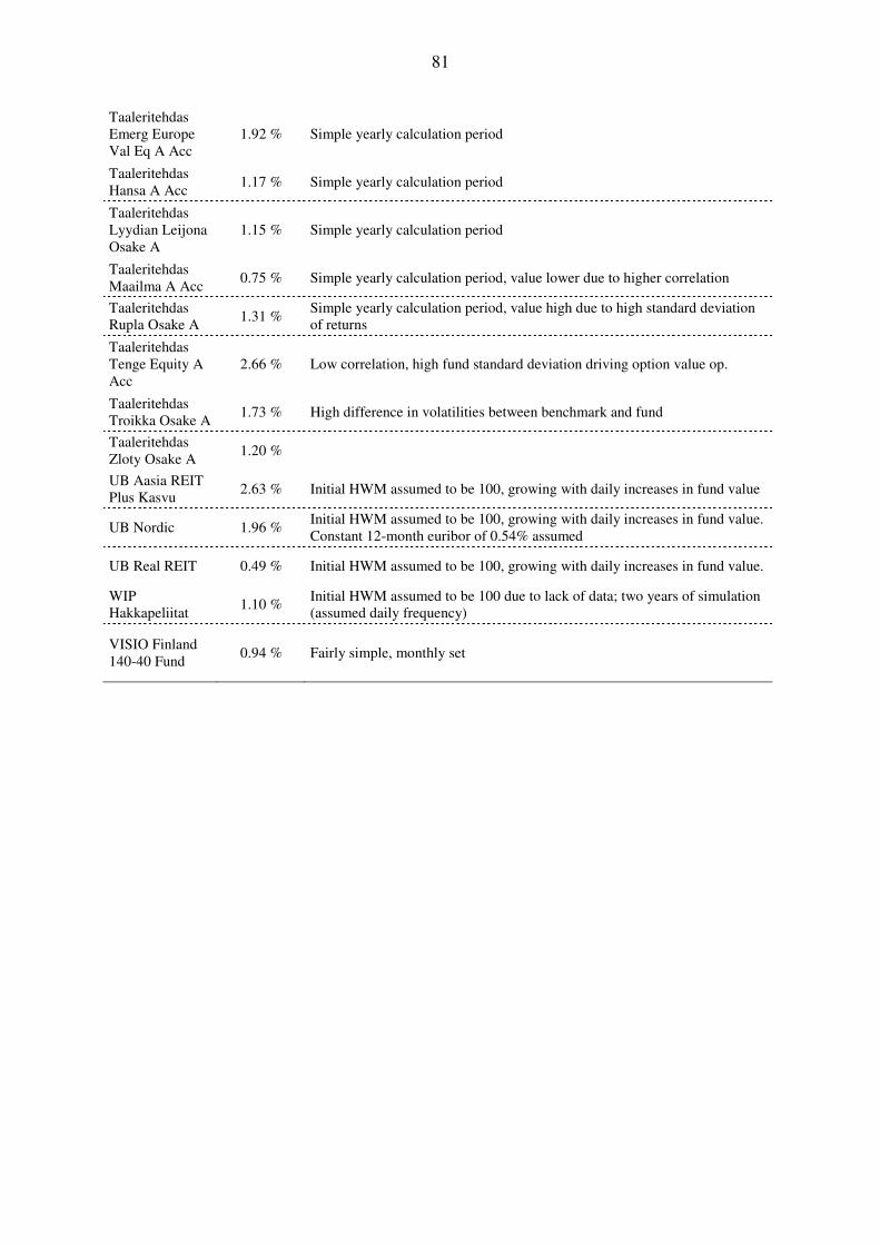
81
Taaleritehdas Emerg Europe Val Eq A Acc
1.92 % Simple yearly calculation period
Taaleritehdas Hansa A Acc
1.17 % Simple yearly calculation period
Taaleritehdas Lyydian Leijona Osake A
1.15 % Simple yearly calculation period
Taaleritehdas Maailma A Acc
0.75 % Simple yearly calculation period, value lower due to higher correlation
Taaleritehdas Rupla Osake A
1.31 % Simple yearly calculation period, value high due to high standard deviation of returns
Taaleritehdas Tenge Equity A Acc
2.66 % Low correlation, high fund standard deviation driving option value op.
Taaleritehdas Troikka Osake A
1.73 % High difference in volatilities between benchmark and fund
Taaleritehdas Zloty Osake A
1.20 %
UB Aasia REIT Plus Kasvu
2.63 % Initial HWM assumed to be 100, growing with daily increases in fund value
UB Nordic 1.96 % Initial HWM assumed to be 100, growing with daily increases in fund value. Constant 12-month euribor of 0.54% assumed
UB Real REIT 0.49 % Initial HWM assumed to be 100, growing with daily increases in fund value.
WIP Hakkapeliitat
1.10 % Initial HWM assumed to be 100 due to lack of data; two years of simulation (assumed daily frequency)
VISIO Finland 140-40 Fund
0.94 % Fairly simple, monthly set