Prepared for submission to JCAP

Dark matter with excitable levels

Andrew J. WrenE-mail: andrew.wren@ntlworld.com

Abstract. This paper explores the possibility that dark matter particles are objects witha set of excitable levels, as for a string or drum. A change in excitation is associated withthe absorption or emission of a photon, and the probability of such a change is dependenton the ambient photon energy density. Particle mass comes entirely from excitations. Suchdark matter with excitable levels, or DMWEL, particles have a distribution of masses whichfreezes out to its present-day form during the early universe. In the particular model consid-ered, consistency with Planck CMB anisotropy observations implies a cautious lower boundon the energy of the first excitable level of 2 to 200 eV for a set of reference parameters.While laboratory detection looks to require a considerable increase in the power of con-trolled light-sources, it might be possible in the near future to detect or constrain DMWELfurther through improved anisotropy observations, closer determination of the CMB’s max-imum deviation from a blackbody shape, or from gravitational probes of the dark matterpower spectrum. For certain parameters near to the boundary of the region allowed by CMBanisotropies, DMWEL dark matter is cold, but with a cut-off halo mass many orders ofmagnitude greater than that typical for WIMP cold dark matter.

Keywords: dark matter theory, cosmology of theories beyond the SM, cosmological param-eters from CMBR, dark matter experiments

ArXiv ePrint: 1912.11453

arX

iv:1

912.

1145

3v3

[as

tro-

ph.C

O]

22

Feb

2020

Contents

1 Introduction 1

2 The model for dark matter with excitable levels 2

3 DMWEL characteristics 43.1 Simplifying assumptions 43.2 Without the simplifying assumptions 6

4 Cosmological constraints 74.1 CMB anisotropies 84.2 CMB energy density and spectrum 94.3 Post-BBN photodissociation of nuclei 114.4 Kinetic decoupling 12

5 Laboratory detection 13

6 Discussion 15

A Validity of the excitation equation 16

B Photodissociation of nuclei 20

References 21

1 Introduction

Following the principle of “leaving no stone unturned” in looking for dark matter [1], thispaper proposes a new dark matter particle, based on the well-known physical phenomenon ofan object having a set of vibrational levels, as for a drum or a string. Atomic electronic transi-tions suggest how changes in occupation of such levels may be associated with the absorptionor emission of photons. This is used as motivation for a model of dark matter particles whichare in principle detectable, but have properties consistent with current observational databecause the transitions are suppressed sufficiently to avoid being obvious in the present day.The model adopted here makes transition probabilities dependent on the ambient photonenergy density — and so, in the cosmological context, on the photon temperature — thephysical idea being that this energy influences the vibrational “tension” in the dark matterparticle. This model is described as dark matter with excitable levels (DMWEL).

As far as the author is able to determine, similar models have not previously been pro-posed. A different notion of excitable levels occurs in models of composite dark matter, suchas dark atoms [2–5], a dark sector analogy of an atom with electron-like levels including, un-like in this paper’s model, the possibility of “ionisation”. Dark atom transitions are associatedwith the emission or absorption, not of photons, but of radiation which is dark to avoid easypresent-day detectability. Dark atoms’ astrophysical detection primarily involves observinginteractions or effects on the evolution of structure [2, 3, 5], but can involve positing smalldark sector-photon interactions [4].

– 1 –

The DMWEL model is motivated by broad analogy with a drum or string; its only linkwith conventional standard model extensions is to borrow the string theoretic idea [see, forexample, 6–9] that mass arises solely from the energy of the excited levels. That assumptionenables the DMWEL model to predict particle mass from basic underlying parameters, andhence, assuming all dark matter is DMWEL, to derive its number density. Note that pro-posed models of dark matter using string theory have recently been reviewed in ref. [10], withthe best tests suggested to be via direct detection experiments and direct collider searches.

This paper’s DMWEL model leads to consideration of several cosmological routes fordetection, relating to the CMB, nuclide abundances, and minimum halo sizes. There mayalso be future prospects for laboratory detection, but these appear more remote.

The paper is arranged as follows. Section 2 describes in more detail the model of darkmatter with excitable levels. Section 3 considers the characteristics of DMWEL particles, in-cluding mass and number density. Section 4 considers cosmological constraints on DMWELparameters, covering in successive subsections, CMB anisotropies, CMB energy density andspectrum, post-BBN photodissociation of nuclei, and kinetic decoupling. Section 5 considerswhether DMWEL might be detected in the laboratory. Section 6 concludes with a discus-sion. Appendices address the validity of the excitation equation (A), and set out detailsrelating to DMWEL’s photodissociation of nuclei (B).

Unless otherwise indicated, all physical constants and quantities are taken from ref. [11].Mathematica and Python calculations used in this paper, including to draw the figures, canbe found in ref. [12].

2 The model for dark matter with excitable levels

This section develops the DMWEL model outlined in the introduction, choosing a particularreference model from the very wide range of possibilities. For simplicity, the energy levelswill be taken to be fermionic in nature, being either empty or occupied. Photon absorptionis associated with a level going from empty to occupied, whilst photon emission is associatedwith going from occupied to empty. For a string or drum, there are two transverse modesof a given energy — for a string, these are in the two orthogonal directions transverse tothe string, and, for a drum, these are transverse vibrations directed along two orthogonaldirections in the drum skin. Motivated by this, DMWEL particles have a pair of levels ofeach given energy. This also accounts for photon polarisations, the levels in a pair beingassociated with orthogonal polarisations.

To detail the model further, assume that the photon background can be consideredas a thermal bath, in the sense that the DMWEL particles have no significant influenceon the photon temperature (this assumption is checked in appendix A for the particularmodel outlined below). Also assume that the photon spectrum does not significantly deviatefrom a pure blackbody spectrum (this will be checked in section 4.2). Consider the emis-sion/absorption probabilities for a given single level from the pair with energy E. Emissionand absorption probabilities can be given by a parameter A, the Einstein coefficient rep-resenting the probability of a spontaneous emission [see, for example, 13]. By a standard“detailed balance” argument, there are two other Einstein coefficients, associated with ab-sorption, BÒ, and stimulated emission, BÓ, equal in value and proportional to A. With the

– 2 –

current conventions, they are related by

BÒ “ BÓ “2π2~3c3

E3 A. (2.1)

The next step is to derive an equation governing the probability that the level is occupied, itsexcitation fraction, f. To ensure this is a straightforward differential equation, the DMWELparticle must have a sufficiently large mass, so that (1) its velocity is non-relativistic, with noneed to account for photons being Doppler-shifted, and (2) its mass is much larger than theenergy of a single transitioning level. These conditions are explored further in section 3.1,and their validity is confirmed for a wide range of parameters in appendix A. Assuming thatthese conditions are satisfied, the energy of the absorbed or emitted photon is equal to thelevel energy E, giving the excitation equation governing f as

dfdt “ BÒ ργ,EpT q p1´ fq ´ rA`BÓ ργ,EpT qs f, (2.2)

whereργ,EpT q “

E3

2π2~3c3`

eE{T ´ 1˘ (2.3)

is the unipolar spectral energy density, that is the differential rate of change of the energydensity with respect to the photon energy, for a particular choice of photon polarisation.

The requirement for emission and absorption to depend on the ambient photon energydensity suggests further setting

A ” A ργeqm.” A T 4, (2.4)

for constants A and A, where the second equivalence holds only if the ambient photons arein thermodynamic equilibrium, in which case their unipolar energy density, totalled over allphoton energies, is given by ργpT q “ π2 T 4{ 30~3c3. Using eqs. (2.1) and (2.4), the excitationequation, eq. (2.2), then becomes

dfdt “ A T 4

˜

1´“

eE{T ` 1‰

f

eE{T ´ 1

¸

, (2.5)

where T is the photon temperature if the photon gas is in thermodynamic equilibrium, or, inother cases, an appropriate effective “excitation temperature”. For practical purposes, it willusually be better to introduce a dimensionless parameter α ” A E4{HpEq, which impliesthat

A “ 9.5ˆ 10´19 eV´4 s´1´ α

10´3

¯

ˆ

E

20 eV

˙´4 ˆ HpEq

Hp20 eVq

˙

, (2.6)

where the eV´4 s´1 quantity was calculated using the Friedman equation [12]. To provide aninitial condition for eq. (2.5), assume that at early times the DMWEL level is in thermody-namic equilibrium with the photon bath — and so for high temperatures fpT q “ feqpT q ”1{ p1` eE{T q. As will be illustrated in section 3.1 and figure 1, this leads to a freeze-out sce-nario, in which, as T declines through T “ E, the level-photon interaction becomes weaker,and the excitation fraction fpT q “freezes out”, becoming appreciably greater than feqpT q,and eventually asymptoting to some effectively constant freeze-out value ffo.

It remains to define the set of levels for the DMWEL particles — the choice of rule forthis is pragmatic, picking a simple rule fairly arbitrarily. Section 1 introduced the assumption

– 3 –

that DMWEL mass comes only from excited levels, so if there were only a single pair oflevels then a fraction p1´ fq2 of the particles would be massless, invalidating the conditionsdescribed after eq. (2.1). Instead, the reference model used in this paper assumes that thereare many level pairs, which are labelled by integers j “ 1, 2, 3, ..., , jmax, where jmax is takento be very large and for practical purposes can be left unspecified (see the end of appendix Afor comment on how large jmax can be). By assumption, the energy of an excitation at a jthlevel, Ej , is proportional to j2, and all the Einstein coefficients, such as Aj , are proportionalto j´2,

Ej “ E1 j2 and, for example, Aj “ A1 j

´2. (2.7)

To close this section, note that with this choice of rules, the inverse j-dependency ofEj and Aj leads to a j invariant, but photon-temperature dependent, tension which can becalculated as [12]

κpT q ”EjAjc

“ 1.0ˆ 10´22 eV cm´1ˆ

T

20 eV

˙4´ α1

10´3

¯

ˆ

E120 eV

˙´3 ˆ HpE1q

Hp20 eVq

˙

, (2.8)

where it was assumed that light speed, c, is the appropriate phase speed. A j- and T -invariantarea can also be constructed, and, in femtobarns, this is

σ ”EjAjc

“ 1.5ˆ 10´2 fb´ α1

10´3

¯

ˆ

E120 eV

˙´3 ˆ HpE1q

Hp20 eVq

˙

, (2.9)

which it is tempting to interpret as a cross section, perhaps associated with the dependencyof emissions and absorptions on the ambient photon energy density.

3 DMWEL characteristics

This section explores characteristics of DMWEL particles. The first subsection makes somesimplifying assumptions, used only in section 3.1 and appendix A. The second subsectionexplores the model further without the simplifying assumptions.

3.1 Simplifying assumptions

For an indicative exploration of DMWEL characteristics it is useful to make the simplifyingassumptions that interest is confined to the radiation-dominated epoch and the number ofrelativistic degrees of freedom g‹ does not depend on temperature. These assumptions strictlyspeaking only apply fully for, say, 20 eV À T À 50 keV, the lower limit ensuring radiationdomination, and the upper limit constant g‹. However, they provide a useful, and not tooinaccurate, qualitative picture outside those limits.

With these assumptions, it is helpful to change the independent variable from t tox “ E{T , noting that dx{dt “ HpT qx “ HpEqx´1, and that the excitation equation eq. (2.5)becomes

dfdx “

α r1´ pex ` 1q f sx3 pex ´ 1q . (3.1)

Figure 1 shows the resulting excitation fraction f for different values of α and x. As thetemperature decreases, x increases and the rate of change of f tends to zero, leading to afreeze-out value ffo of the excited fraction. Figure 2 shows ffo as α varies. Note also thatthe simplifying assumptions, with eq. (2.7) and the definition of α before eq. (2.6), implyαj “ α1 j

2.

– 4 –

0.1 1 10 100

10-6

10-5

10-4

10-3

10-2

10-1

1

Figure 1: The freeze-out process as x varies, for selected of values of α. The function f isthe fraction of DMWEL particles for which the level is excited. The dashed line, feq, withfeqpxq “ 1{ p1` exq, shows the excited fraction in equilibrium, which, assuming equilibrium,is independent of α. The figure makes the simplifying assumptions of section 3.1.

10-5 10-4 10-3 10-2 10-1 100 101 102 103

10-6

10-5

10-4

10-3

10-2

10-1

1

Figure 2: The excitation fraction at freeze-out, as a function of α, with the simplifyingassumptions of section 3.1.

Recall that the DMWEL particle mass comes exclusively from excitation energies. Eachof a DMWEL particle’s levels has an independent probability of excitation, so the particlemass is not fixed, but follows a distribution given by

m “ 2E1ÿ

j

j2Fj , (3.2)

where Fj “ 0, 1{2, or 1, depending on whether neither, exactly one, or both the pair of jthlevels are excited. For sufficiently large x1, the mass will freeze out to a distribution which

– 5 –

0 1×107 2×1070.000

0.005

0.010

0.015

0 0.5×106 1.0×1060.000

0.001

0.002

0.003

0 20000 40000 600000.000

0.002

0.004

0.006

0 500 1000 1500 20000.000

0.010

0.020

0.030

0.040

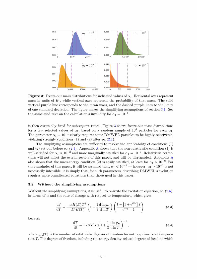
Figure 3: Freeze-out mass distributions for indicated values of α1. Horizontal axes representmass in units of E1, while vertical axes represent the probability of that mass. The solidvertical purple line corresponds to the mean mass, and the dashed purple lines to the limitsof one standard deviation. The figure makes the simplifying assumptions of section 3.1. Seethe associated text on the calculation’s invalidity for α1 “ 10´1.

is then essentially fixed for subsequent times. Figure 3 shows freeze-out mass distributionsfor a few selected values of α1, based on a random sample of 106 particles for each α1.The parameter α1 “ 10´1 clearly requires some DMWEL particles to be highly relativistic,violating strongly conditions (1) and (2) after eq. (2.1).

The simplifying assumptions are sufficient to resolve the applicability of conditions (1)and (2) set out before eq. (2.1). Appendix A shows that the non-relativistic condition (1) iswell-satisfied for α1 ď 10´3 and more marginally satisfied for α1 “ 10´2. Relativistic correc-tions will not affect the overall results of this paper, and will be disregarded. Appendix Aalso shows that the mass-energy condition (2) is easily satisfied, at least for α1 ď 10´2. Forthe remainder of this paper, it will be assumed that, α1 ď 10´2 — however, α1 ą 10´2 is notnecessarily infeasible, it is simply that, for such parameters, describing DMWEL’s evolutionrequires more complicated equations than those used in this paper.

3.2 Without the simplifying assumptions

Without the simplifying assumptions, it is useful to re-write the excitation equation, eq. (2.5),in terms of α and the rate of change with respect to temperature, which gives

dfdT “ ´

αHpEqT 3

E4HpT q

ˆ

1` 13

d ln g‹sd lnT

˙

˜

1´“

1` eE{T‰

f

eE{T ´ 1

¸

, (3.3)

becausedTdt “ ´HpT qT

ˆ

1` 13

d ln g‹sd lnT

˙´1, (3.4)

where g‹spT q is the number of relativistic degrees of freedom for entropy density at tempera-ture T. The degrees of freedom, including the energy density-related degrees of freedom which

– 6 –

-4.0 -3.5 -3.0 -2.5 -2.0

1

2

3

4

-1

0

1

2

3

4

5

6

-4.0 -3.5 -3.0 -2.5 -2.0

1

2

3

4

-9

-8

-7

-6

-5

-4

-3

-2

Figure 4: For selected DMWEL parameters, mass after freeze-out (left) and present-daynumber density (right).

determine H, are taken from data on the standard model in refs. [11, 14].1 Any additionalhigh energy non-standard model relativistic degrees of freedom would have to be very largein number to have a significant effect.

Without the simplifying assumptions, from the definition of α before eq. (2.6), αj isgiven by

αj “α1 j

6HpE1q

HpEjq. (3.5)

The mean mass over all DMWEL particles at a given temperature T is then

mpT q “ 2E1ÿ

j

j2fpαj , E1j2, T q, (3.6)

and for low enough temperatures the mass has frozen out at an essentially constant value.Assuming that DMWEL particles make up all dark matter, the present-day DMWEL num-ber density would then be n0 “ ρdm,0{ mfo, the present-day mass density divided by themean freeze-out mass. The present-day DMWEL particle mass and number density can becalculated numerically [12], and are shown for selected parameters in figure 4. The resultsfor the number density enable verification in appendix A that, as assumed at the start ofsection 2, the photon background acts as a thermal bath, with DMWEL minimally affectingphoton temperatures, except at very high temperatures of order 105 GeV.

4 Cosmological constraints

This section considers cosmological constraints, arising from CMB anisotropies, the CMBenergy density and spectrum, post-BBN photodissociation of nuclei, and from kinetic decou-pling. Planck CMB anisotropy constraints emerge as the tightest.

1The quark-hadron transition is taken to occur at 160 MeV, in the middle of the range 150 to 170 MeVoften quoted.

– 7 –

4.1 CMB anisotropies2

Emission of photons in the early universe would have affected CMB anisotropies [15–22], soPlanck observations, most recently updated in ref. [22], can constrain DMWEL parameters.Such photons affect the intergalactic medium (IGM) through various “channels”, of whichionisation of hydrogen atoms and heating of the IGM are significant for CMB anisotropies [16,19, 20]. Reference [22] considered a model of dark matter self-annihilation and derived a one-sigma constraint on the self-annihilation strength. Here this constraint is used to deriverelated constraints for DMWEL dark matter’s first energy level E1, for given α1.

If Dc is the energy per comoving unit volume deposited by DMWEL into channel c atredshifts below z, then,

dDcdz “ n0pα1, E1q

ÿ

j

2fDc, jpzqEj

dfjdz , (4.1)

where fDc, jpzq is the power deposited in channel c at redshift z, having come originally from

one of the jth levels, divided by the photon emission power of that level at redshift z. Similarlyfor dark matter self-annihilation, the corresponding rate is given by [21]

dDann, cdz “

χc pann ρ2dm,0 p1` zq

2

Hpzq, (4.2)

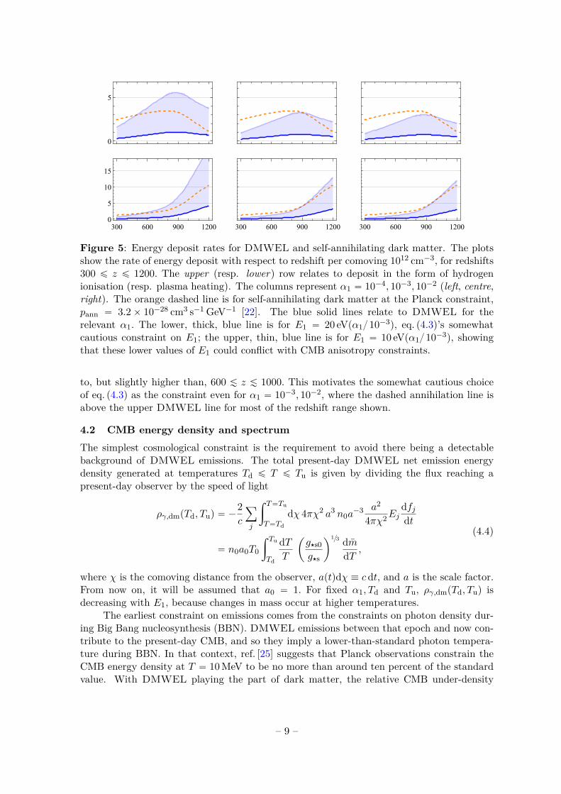
where χc is the fraction of the deposited energy that goes into channel c, and pann is a co-efficient representing the self-annihilation strength. The most recent Planck results [22] givea 95%-confidence maximum of pann “ 3.2ˆ 10´28 cm3 s´1 GeV´1, similar to, but slightlytighter than, the pann “ 3.4ˆ 10´28 cm3 s´1 GeV´1 constraint from the Planck 2015 re-lease [21].3 The rates for DMWEL and self-annihilation will turn out to have a broadlysimilar redshift dependency which will justify seeking values of pα1, E1q giving similar ratesof energy deposit to those arising from the constraint value of pann from ref. [22]. This avoidsdoing a full Monte Carlo analysis of DMWEL emissions and cosmological parameters, asused in ref. [22] to find pann, providing instead a more direct comparison of the DMWELand self-annihilation models.

The comparison of eqs. (4.1) and (4.2) can be facilitated by modifying slightly [12]the DarkAges package [23] from the ExoCLASS branch of CLASS [24] to calculate the sum ineq. (4.1) for DMWEL, via eq. (3.3). It can be found numerically that dDc{dz is decreasingwith E1 over the parameter range used in figure 4, and at least down to E1 “ 10´2 eV [12]. Inparticular, results shown in figure 5 indicate that, for 10´4 ď α1 ď 10´2, a cautious estimateof the minimum E1 compatible with Planck observations is given by

E1,min “´ α1

10´3

¯

20 eV. (4.3)

In interpreting figure 5, note that CMB anisotropies are most sensitive to self-annihilationenergy deposit in the range 600 À z À 1000 [21]. DMWEL energy deposit’s variation withredshift is similar to that for self-annihilation, but slightly more biased to higher redshifts,suggesting that the greatest sensitivity to DMWEL emissions is in a redshift range similar

2Based on observations obtained with Planck (http://www.esa.int/Planck), an ESA science mission withinstruments and contributions directly funded by ESA Member States, NASA, and Canada.

3The parameter pann accounts for the total proportion of the energy which is deposited into the IGM [22,eq. 87], which is why χc rather than fDc appears in eq. (4.2).

– 8 –

0

5

300 600 900 12000

5

10

15

300 600 900 1200 300 600 900 1200

Figure 5: Energy deposit rates for DMWEL and self-annihilating dark matter. The plotsshow the rate of energy deposit with respect to redshift per comoving 1012 cm´3, for redshifts300 ď z ď 1200. The upper (resp. lower) row relates to deposit in the form of hydrogenionisation (resp. plasma heating). The columns represent α1 “ 10´4, 10´3, 10´2 (left, centre,right). The orange dashed line is for self-annihilating dark matter at the Planck constraint,pann “ 3.2ˆ 10´28 cm3 s´1 GeV´1 [22]. The blue solid lines relate to DMWEL for therelevant α1. The lower, thick, blue line is for E1 “ 20 eVpα1{ 10´3q, eq. (4.3)’s somewhatcautious constraint on E1; the upper, thin, blue line is for E1 “ 10 eVpα1{ 10´3q, showingthat these lower values of E1 could conflict with CMB anisotropy constraints.

to, but slightly higher than, 600 À z À 1000. This motivates the somewhat cautious choiceof eq. (4.3) as the constraint even for α1 “ 10´3, 10´2, where the dashed annihilation line isabove the upper DMWEL line for most of the redshift range shown.

4.2 CMB energy density and spectrum

The simplest cosmological constraint is the requirement to avoid there being a detectablebackground of DMWEL emissions. The total present-day DMWEL net emission energydensity generated at temperatures Td ď T ď Tu is given by dividing the flux reaching apresent-day observer by the speed of light

ργ,dmpTd, Tuq “ ´2c

ÿ

j

ż T“Tu

T“Td

dχ 4πχ2 a3 n0a´3 a2

4πχ2Ejdfjdt

“ n0a0T0

ż Tu

Td

dTT

ˆ

g‹s0g‹s

˙1{3 dmdT ,

(4.4)

where χ is the comoving distance from the observer, aptqdχ ” c dt, and a is the scale factor.From now on, it will be assumed that a0 “ 1. For fixed α1, Td and Tu, ργ,dmpTd, Tuq isdecreasing with E1, because changes in mass occur at higher temperatures.

The earliest constraint on emissions comes from the constraints on photon density dur-ing Big Bang nucleosynthesis (BBN). DMWEL emissions between that epoch and now con-tribute to the present-day CMB, and so they imply a lower-than-standard photon tempera-ture during BBN. In that context, ref. [25] suggests that Planck observations constrain theCMB energy density at T “ 10 MeV to be no more than around ten percent of the standardvalue. With DMWEL playing the part of dark matter, the relative CMB under-density

– 9 –

α1 10´4 10´3 10´2 FIRAS upper boundE1{ eV 2 20 200

µ 2ˆ 10´7 1ˆ 10´7 1ˆ 10´7 9 ˆ 10´5

y 5ˆ 10´10 4ˆ 10´10 3ˆ 10´10 1.5ˆ 10´5

Table 1: The µ and y parameters for selected α1 and the corresponding E1 from theanisotropy constraints, displayed alongside the p95%-confidence) observational upper boundsfrom FIRAS [27].

at T “ 10 MeV, compared with its standard density, is ργ,dmpT0, 10 MeVq{ ργpT0q. Calcula-tions [12] then show that this quantity is less than 10´4 for values of α1 and E1 compatiblewith the anisotropy constraints of eq. (4.3), and so DMWEL parameters are not furtherconstrained by effects during BBN.

Photon emissions at temperatures above around 500 eV are rapidly thermalised andaffect only the blackbody temperature, not the CMB spectrum [26]. However, later emissionsmay result in distortions to the CMB spectrum, which observations closely constrain to ablackbody spectrum [26–28]. Useful approximations for this effect are given in ref. [29],taking account of the two possible types of primordial distortions, so-called µ-type and y-type distortions. The simplest approximation considers separately the energy-release in the µ-epoch, which is taken to be Tth ” 500 eV ą T ą 10 eV ” Tµy, and in the y-epoch, 10 eV ą T ą0.26 eV ” Trec, the latter being the temperature at recombination. The respective spectraldistortions are characterised via parameters which are given in the simplest approximationby [26, 29]

µ ” 1.401∆ργργ

ˇ

ˇ

ˇ

ˇ

µ

“1.401n0 T0ργpT0q

ż Tth

Tµy

dTT

dmdT (4.5)

and

y ”14

∆ργργ

ˇ

ˇ

ˇ

ˇ

y

“n0 T0

4ργpT0q

ż Tµy

Trec

dTT

dmdT . (4.6)

The results [12] in table 1 show that the relevant observational upper bounds from FIRAS [27]allow E1 “ E1,min for 10´4 ď α1 ď 10´2, and so also all greater E1. In other words, theexisting µ and y constraints are much weaker than those from CMB anisotropies. However,the µ-distortions of table 1 are close to 5σ-detectable by the proposed PIXIE instrument [30,fig. 12 and the associated discusssion], and well within 5σ-detectability of the further proposedSuper-PIXIE [31], while the y-distortions are some way beyond both PIXIE and Super-PIXIE’s 1σ-sensitivity [30, 31].

It remains to quantify the spectrum of DMWEL emissions following recombination,via the intensity I, the incident radiation power per unit spectral energy per unit area persteradian. The intensity at spectral energy E associated with the jth pair of levels comesfrom emissions at temperature Tj “ EjT0{E and, from eqs. (4.4), (3.3) and (3.5), is

IjpEq “c

4π2n0T0Ej

Tj

dfjdT

ˇ

ˇ

ˇ

Tj

dTjdE “

cn0T40α1HpE1qj

6ffo,j2πE4HpTjq

, (4.7)

– 10 –

●

●● ● ●

●

■

■

■ ■ ■ ■■

▲

▲

▲ ▲ ▲▲

▲▲

◆◆ ◆ ◆ ◆

◆◆ ◆

◆ ◆

◆◆

◆◆

◆

◆

10-15 10-12 10-9 10-6 10-310-12

10-9

10-6

10-3

100

103

◆

● 10-2

■ 10-3

▲ 10-4

Figure 6: Comparing the spectral energy times the intensity of extragalactic backgroundlight (EBL) [32] and DMWEL emissions for selected values of wavelength λ. The DMWELparameters for the indicated α1, with corresponding E1 “ 20 eV

`

α1{ 10´3˘ .

while the total intensity at spectral energy E comes from summing the over all j for whichE{E1 ď j2 ď TrecE{ pT0E1q. The results [12] are shown in figure 6, which compares theresulting intensity for the minimum anisotropy parameters of eq. (4.3), with that of theextragalactic background light (EBL) [32]. For relevant wavelengths near the DMWEL peakin figure 6, larger values of E1 give values of E I which are lower.4 Note that, for the DMWELparameters plotted in the figure, the peak of DMWEL emissions strength is in a part ofthe ultraviolet where there is little observational data due to the absorption of this radiationby neutral hydrogen (this corresponds to the gap in the plotted EBL wavelengths aroundλ “ 10´8 to 10´7 m´1) [32]. Nonetheless, figure 6 clearly implies that post-recombinationDMWEL emissions are unobservable.

4.3 Post-BBN photodissociation of nuclei

Photodissociation of light nuclei arises from gamma radiation with energies of at least aroundEγ “ 1.5 MeV [33, 34] trigger photodissociation at temperatures sufficiently low that thesegamma rays no longer produce electron and positron pairs on CMB photons. The pairproduction threshold temperature is approximated by T “ m2

e{ 22Eγ [35–38], which is alittle less than 10 keV for Eγ “ 1.5 MeV, implying that for all relevant level energies, theexcitation fractions have frozen out to ffo,j , enabling the rightmost round round-bracketedterm in eq. (3.3) to be replaced by ´ffo,j . Appendix B describes detailed photodissociationcalculations based on a recently developed approach [39, 40] for emissions of energy less thataround 100 MeV. The appendix shows that photodissociation due to DMWEL is of negligiblesignificance, at least for 10´4 ď α1 ď 10´2 and the values of E1 allowed by CMB anisotropies.Deuterium is the nuclide most sensitive to DMWEL emissions, and observational error wouldneed to be reduced by more than ten times in order for deuterium abundance to improve theconstraints from CMB anisotropies.

4This can be checked using ref. [12].

– 11 –

-4.0 -3.5 -3.0 -2.5 -2.0

1

2

3

4

4.5

5.0

5.5

6.0

6.5

7.0

7.5

8.0

8.5

Figure 7: Kinetic decoupling temperatures for a range of DMWEL parameters.

4.4 Kinetic decoupling

Kinetic decoupling — which influences the matter power spectrum — occurs when photon-dark matter interactions are no longer frequent enough to maintain dark matter particlesat momenta associated with the photon temperature, p “

?2mT, within a Hubble time,

H´1 [41–43]. From eq. (2.5), the rate per unit time for emissions and absorptions from thepair of levels j is given by

re j “2A1j

´2 T 4 eEj{T fpαj , Ej , T qeEj{T ´ 1

and ra j “2A1j

´2 T 4 p1´ fpαj , Ej , T qqeEj{T ´ 1

(4.8)

respectively, and in either case the size of the momentum change is the same, ∆p “ Ej . Theoverall rate of variance in DMWEL momentum is then the sum over j of pre j ` ra jqE2

j .From eqs. (4.8) and (3.5), the time period trelax over which that variance totals to the squareof the typical kinetic equilibrium momentum is given by

trelax

ˆ

2α1HpE1qT4

E21

˙

ÿ

j

j2ˆ

1eEj{T ´ 1

` fpαj , Ej , T q

˙

“ 2mT. (4.9)

Kinetic decoupling occurs when the relaxation time becomes as long as the Hubble time,trelax “ HpT q´1, so eq. (4.9) means that the kinetic decoupling temperature Tkd satisfies

ÿ

j

2j2

eEj{Tkd ´ 1“mpTkdq

E1

ˆ

E31HpTkdq

α1T 3kdHpE1q

´ 1˙

, (4.10)

and the resulting Tkd are shown in figure 7.There are three different scales associated with kinetic decoupling which each make a

cut-off in the power spectrum for dark matter perturbations. These scales are produced byacoustic oscillations, free-streaming and damping, with comoving wave numbers kao, kfs and

– 12 –

kd respectively. The dominant effect comes from the largest length scale of the three, whichis the one with smallest comoving wave number. The acoustic oscillation scale [42] is givenby

kao “ πakdHkd, (4.11)

while the free-streaming scale is [41]

kfs “

ˆ

m

Tkd

˙1{2paeq{ akdq

ln p4aeq{ akdqkeq, (4.12)

where keq is the comoving Hubble parameter and aeq the scale factor at radiation-matterequality, both being taken from ref. [22].5 The damping scale is given by [41]

kd “

ˆ

32

ż tkd

0

T trelaxma2 dt

˙´ 1{2

, (4.13)

where tkd is the time of kinetic decoupling, and the integral is evaluated numerically, afterchanging the integration variable to lnT [12]. The resulting mass cut-off scale is then

Mcut “4π3 ρdm,0

ˆ

π

min pkao, kfs, kdq

˙3, (4.14)

and this is shown for selected DMWEL parameters in figure 8. Over the parameter spacedisplayed, the cut-off mass comes from acoustic oscillations or free-streaming. The largestcut-off masses occur at the CMB anisotropy constraints, being of order 104 M@. For compar-ison, cut-off masses for WIMPs are typically much smaller, ranging up to around 102 MC „

3ˆ 10´4 M@ [44]. Figure 8’s DMWEL cut-off masses do not conflict with Lyman-α forestconstraints for the cut-off at around 1hMpc´1 [45, 46], corresponding to Mcut “ 1013 M@.Nor do they conflict with maximum cut-off masses of 107 to 108 M@ recently derived usingquasar gravitational lensing [47] and from Gaia and Pan-STARRS observations of stellarstreams [48].

Possible approaches to observing cut-off masses are discussed in refs. [42, 43]. Someof these seek signals from dark matter annihilation boosted by halo densities, and so arenot applicable to DMWEL. Others involve the detection of dark matter halos through theirgravitational effects, and are relevant. For example, it might be possible to confirm a lack ofhalos below a cut-off mass through gravitational lensing [49, 50] or through Doppler effectson millisecond pulsar timing measurements, which could potentially be probed via the SKAand follow-up observations [51].

5 Laboratory detection

Detecting DMWEL in astrophysical contexts would be difficult, requiring a hot, dense elec-tromagnetic environment, in combination with the possibility of detecting emission or absorp-tion of photons by the (fairly sparse) DMWEL particles, against that bright, hot background.This suggests laboratory detection as potentially a better prospect, because detection couldbe optimised in a controlled environment.

5The mass explicitly appearing in eq. (4.12) is the freeze-out mass which affects the final free-streaming,and is a little smaller than the mass at temperature Tkd.

– 13 –

-4.0 -3.5 -3.0 -2.5 -2.0

1

2

3

4

-10

-8

-6

-4

-2

0

2

4

Figure 8: Cut-off masses, Mcut, for a range of DMWEL parameters. The black line dividesparameters where the cut-off is determined by the acoustic oscillation (“AO”) scale, kao, ofeq. (4.11), from those where it is determined by the free-streaming scale, kfs, of eq. (4.12).

The present-day local dark matter density at the Earth is estimated as ρdm,0 δCdm “

0.5 GeV cm´3 [11, 52]. The imagined experiment, motivated by ref. [53], uses a powerfulphoton source, such as an X-ray free-electron laser (XFEL) [54], to generate a high enoughenergy density for spontaneous DMWEL emissions to be observed. In a configuration withlaser photons of energy 1680 eV, the European XFEL [55] can generate an average power ofPEX “ 1.6ˆ 1021 eV s´1, which is distributed via 27 000 photon bunches per second [56].

Looking for spontaneous emissions, from eqs. (2.4) and (2.5) there would be an emissionrate for the jth pair of levels,

Ej “2n0 δ

Cdm Aj PLffo,j

c

“ j´2´ α1

10´3

¯

˜

n0n0|α1“10´3, E1“20 eV

¸

ˆ

ffo,j0.5

˙ˆ

P

PEX

˙ˆ

L

1 m

˙

5ˆ 10´11 yr´1,

(5.1)

for average power P, where L is the length of the beam surrounded by a cylindrical detectorof DMWEL emissions.6 In order to generate a few first level emissions per year, the power(times the detector length) needs to be increased by a factor of 1011, and, because

ř

j j´2 «

1.6, emissions from higher levels make little difference. Increasing the power compared withthe European XFEL would involve one or both of increasing the energy in each photonbunch and increasing the proportion of the time during which XFEL photons are generated(assuming that a photon bunch typically has a duration of, say, 2ˆ 10´14 s [57], photons areonly being emitted by the European XFEL for 5ˆ 10´10 of its operational time). Note thatthe coherence of the beam is not important, nor need the collimation of the beam be very

6Note that this does not depend on any assumption about the excitation temperature of the DMWELlevels, which was defined after eq. (2.5).

– 14 –

tight, however it does need to be free of photons of energy Ej , and the detection volumeneeds to be very well-shielded, in order to avoid any background photons of energy Ej . Insummary, this section suggests that it is not yet possible to detect DMWEL dark matter ina laboratory, and to do so would require a considerable increase in the power of controlledlight-sources.

6 Discussion

This paper considered a form of dark matter with excitable levels, DMWEL, for whichthe emission and absorption rates are proportional to the ambient photon energy density.Beyond this interaction with photons, there is no direct link with the standard model ofparticle physics, however, the model reflects familiar physical notions of energy levels andtheir excitation, adding an extra ingredient of dependence on the ambient environment, whichcan be associated, in eqs. (2.8) and (2.9), with a physical tension and cross section.

For the particular model adopted, the strongest parameter constraints come from Planckobservations of CMB anisotropies [22]. Better constraint, or detection, via the abundanceof light elements, or through laboratory methods, does not appear particularly plausible inthe near future — and constraint or detection of DMWEL by observing emissions sincerecombination seems impossible. The Planck constraints could be improved, or DMWELdetected, via improved anisotropy observations, better observations of the CMB spectrum [30,31, 58], or by detecting gravitational effects from the cut-off DMWEL would induce in thedark matter power spectrum [49–51].

DMWEL gives a viable model of dark matter, which can be tested by observation.Appendix A confirms that, with parameter α1 ď 10´2, DMWEL is cold dark matter, andsection 4.4 finds that, for parameters near to the boundary of the region allowed by CMBanisotropies, the associated dark matter power spectrum cut-off mass is many orders ofmagnitude greater than that typical for WIMP cold dark matter.

As noted at the end of appendix A, at very early times DMWEL with extremely largenumbers of levels will be sufficiently massive that level-occupation stores all or almost allthe energy that later is in the radiation background. It is tempting to associate this withan end to inflation somewhat different to the usual reheating scenario, with kinetically coldDMWEL particles storing all the subsequent radiation heat. The implications of this couldbe explored further.

This paper has focused on a part of DMWEL parameter space where the Einstein coef-ficients are sufficiently low, corresponding to α1 ď 10´2, to ensure that DMWEL occupationfractions can be modelled via a differential equation, eq. (2.5). In particular, this is associatedwith the DMWEL particles being sufficiently non-relativistic even at the time in the earlyuniverse when the ratio of DMWEL mass over photon temperature is at a minimum. Itshould be possible to develop an approach for calculating the evolution of DMWEL particleswith parameter α1 ą 10´2, based on eq. (A.3), and explore the associated dark matter which,since the particle mass would follow a distribution at least roughly like that of figure 3 (bot-tom right), looks likely to be a mixture of dark matter of varying warmth. It would also bepossible to use eq. (2.5) to explore lower α1 parameters than those considered in this paper,α1 ă 10´4 allowing first energy levels E1 lower than 2 eV.

Alternative models along DMWEL lines could, of course, be constructed. There arelimitless possible choices of rules characterising the temperature dependence, set here ineq. (2.4), and the j dependence of the energy and Einstein coefficients, see eq. (2.7). It

– 15 –

would also be possible, for example, to replace the assumption that the levels are fermionic(occupation number zero or one) and make them instead bosonic (occupation characterisedby a non-negative integer), or indeed adopt some other occupation rule. Another variantwould be to associate a level change with absorption or emission of a particle other than aphoton. Wanting the dark matter to be plausibly detectable might suggest this should be aneasily detectable particle, such as an electron, instead of, say, a neutrino which might alwayspass undetected.

Another approach would be to explore DMWEL-like models for which level occupationfreezes in, rather than, as in this paper, freezes out. Instead of starting in equilibrium at hightemperatures and undergoing net emission, dark matter would begin with levels unoccupiedat high temperatures, and absorb photons over time. This would imply greater photon densityat early times relative to the standard cosmological model, and it is perhaps conceivable thatsuch a model could explain the difference between values of the Hubble parameter detectedvia early universe and local universe methods [59–65].

In conclusion, this paper considered a new type of dark matter model, developing anexample that was found to be consistent with observational data and potentially detectablein the near future. Referring back to the start of section 1, this indicates new “stones” toturn over in looking for dark matter [1].

Appendices

A Validity of the excitation equation

As indicated after eq. (2.1), for the excitation equation eq. (2.5) to be valid, the DMWELparticle must (1) be sufficiently non-relativistic that the the Doppler effects on the total andspectral photon energy density are not significant. It is also necessary (2) that its mass ismuch greater than the level energy, in order to avoid the energy of absorbed or emittedphotons being too different from the corresponding DMWEL level energy. This appendixexplores the validity of these conditions, together the validity of the assumption, set out at thestart of section 2, that DMWEL particles do not significantly affect the photon temperature.

This appendix focuses on α1 “ 10´2, 10´3 and 10´4. Figure 3 shows that for α1 “ 10´1,at least some DMWEL particles are relativistic, and so the excitation equation is not strictlyvalid. The results for α1 “ 10´4 will show that the excitation equation is clearly valid forlesser values of α1.

Figure 9 shows mass over temperature ratios r “ m{T for DMWEL particles withα1 “ 10´2, 10´3 and 10´4, indicating, for each x1, the mean ratio and one-standard-deviationrange of r. The lower end of those ranges has a minimum of around r “ 20, 90 and 300 forα1 “ 10´2, 10´3, 10´4 respectively. For convenience, in this appendix choose units so thespeed of light c “ 1. Then the velocity distribution of DMWEL particles can be found fromthe relativistic gamma factor γ “

`

1´ v2˘´ 1{2, which follows a Maxwell-Jüttner distribution

given by

Jpγq “r γ2v

K2prqexpp´r γq, (A.1)

where K2 is a Bessel K-function.

– 16 –

●●

●●

●●●●●●●●●●●

●

●

●

●

■■

■■■■■■■■■■

■■

■

■

■

■

■

▲▲

▲▲▲▲▲▲▲▲▲▲

▲

▲

▲

▲

▲

▲

10-6 0.001 1

10

1000

105

107

● 10-2

■ 10-3

▲ 10-4

Figure 9: The ratio r of mass divided by temperature for the indicated values of α1 andx1. The discs, triangles and squares show mean values, with the associated vertical linesindicating one standard deviation.

A DMWEL particle with a velocity v relative to the photon background can betaken [66–69] to have a spectral energy density with effective temperature given by

Teff “T?

1´ v2

1´ v cospθq , (A.2)

where v “ ‖v‖, and θ is the angle between v and the direction of the photon observed fromthe particle. Considering the excitation equation, eq. (2.5), this leads to a relativistic versionof eq. (3.1),

dfdx “

α

x3

«C

pTeff{T q4

epT {Teffqx ´ 1

G

´

C

pTeff{T q4 `epT {Teffqx ` 1

˘

epT {Teffqx ´ 1

G

f

ff

, (A.3)

where, for any function qpv, θq,

xqy ”

ż 8

1dγ Jpγq

ż π

0

dθ sinpθq2 qpvpγq, θq (A.4)

takes the appropriately-weighted average over all relativistic gamma factors γ and angles θ.Equations (A.1) and (A.2) enable calculation [12] of the two angle-bracketed coefficients

on the right-hand side of eq. (A.3). Figure 10 compares these with eq. (3.1)’s correspondingnon-relativistic coefficients, and in interpreting the figure it should be noted that, for x Á 1,the coefficient for the f -independent term is exponentially suppressed relative to that for thef -dependent term. However, for 0.1 À x À 1, relativistic effects increase the coefficient of thef -independent term in eq. (A.3) more than the f -dependent term, and so tend to increasefreeze-out values. A rough calculation of the effect on DMWEL mass can be made usingthe data in figures 9 and 10, and this suggests that, for α1 “ 10´2, the mass is increased bysomewhere between 30 and 60 percent, equivalent to 0.1 to 0.2 dex, while, for α1 “ 10´3, the

– 17 –

0.001 0.010 0.100 1 10

1.0

1.2

1.4

1.6

1.8

2.0

0.001 0.010 0.100 1 10

1.0

1.2

1.4

1.6

1.8

2.0

Figure 10: The ratio of angle-bracket coefficients from the relativistic equation eq. (A.3)over the corresponding non-relativistic coefficients from eq. (3.1). The plots are (left) for thefirst angle-bracket coefficient, associated with the f -independent term, and (right) for thesecond angle-bracket coefficient, associated with the f -dependent term.

mass increase is around 10 percent. The effects on emission-absorption processes, importantin sections 4 and 5, may well be less, as emissions and absorptions per DMWEL particlewill increase, while the particle number density decreases. The conclusion is that condition(1) can be assumed to be satisfied for α1 ď 10´2, albeit possibly somewhat marginally rightat the upper end of that range. In any case, such corrections will not affect the overall —order of magnitude — results in this paper, and will be disregarded.

Now consider condition (2) to verify that for a stimulated emission or absorption thephoton energy Eγ is essentially the same as the level energy E.When a stationary DMWELparticle absorbs a photon into a level of energy E, conservation of energy and momentumimplies that

Eγ “ E

ˆ

1` E

2m

˙

, (A.5)

whilst stimulated emission from a stationary DMWEL particle7 yields a photon of energy

Eγ “ E

ˆ

1` E

2 pm` Eq

˙

. (A.6)

Absorption therefore implies a slightly tighter condition than simulated emission on E{min order to ensure Eγ « E. Considering eqs. (2.2) and (3.1), the combined rate of either anabsorption or stimulated emission is given by

drcdx “

α

x3 pex ´ 1q . (A.7)

Figure 11 shows the energy-weighted probability that an absorption or stimulated emissionfrom a DMWEL particle is from a level j that exceeds the arbitrary tolerance of Ej{ 2m ě

0.01,

Px1 “

¨

˝

ÿ

pEj{ 2mqě0.01Ej

drc jdx1

˛

‚

N

˜

ÿ

jě1Ej

drc jdx1

¸

. (A.8)

7Noting that coherence of stimulated emission implies the emitted photon has the same energy and mo-mentum as the stimulating photon.

– 18 –

●●●●●●●●●●●●●

●

●

●

●■

■■■■■ ■ ■ ■

■

■

■▲▲ ▲

▲

10-6 10-4 0.01 1

10-12

10-10

10-8

10-6

10-4

0.01● 10-2

■ 10-3

▲ 10-4

Figure 11: The probability Px1 as described in eq. (A.8), for selected α1 and x1.

Figure 11 indicates that such absorptions or stimulated emissions, with Eγ ff E, are of min-imal significance.

It remains to check that the photon temperature is not significantly affected by DMWELparticles, at least other than for very high temperatures. From figure 1, for large αj (sayαj Á 100), a useful approximation to fj is that it is 1{2 for xj À 1 and 0 for xj Á 1 (asan aside, but also as an accuracy check, this approximation can be used to explain the co-incidence of low x1 points for differing α1 in figure 9). The high-jth level pairs will emit, ataround x „ 1, a photon energy per physical unit volume

Ej “ 2Ejn0E3j

T 30. (A.9)

The transitioning level-number jpT q at photon temperature T is given by jpT q “a

T {E1,and this gives an expression for the rate of change of radiation energy density with respectto temperature which includes the standard term 4ρ‹{T , and an additional term for theDMWEL effects,

dρ‹dT “

4ρ‹T´

Ej

gγ?TE1

, (A.10)

where gγ is the number of particle degrees of freedom in thermal equilibrium with photons,which is assumed to be constant at the maximum standard model value of gγ “ 427{4 [11].This can be solved analytically [12] to give

ρ‹pT q

1036 GeV cm´3 “

«

5ˆ 106 ` 1ˆ 103ˆ

E120 eV

˙´ 1{2 ˆ n0n0 ‚

˙

ff

ˆ

T

GeV

˙4

´ 8ˆ 101ˆ

E120 eV

˙´ 1{2 ˆ n0n0 ‚

˙ˆ

T

GeV

˙9{2

,

(A.11)

with n0 ‚ ” n0|α1“10´3, E1“20 eV. Note, from figure 4 (right), that n0 ‚ is, to order of magni-tude, the biggest DMWEL number density compatible with section 4.1’s CMB anisotropyconstraints. This implies the second coefficient of T 4 in eq. (A.11) is always negligible.

– 19 –

From eq. (A.11), it can be found that for

T ď

ˆ

E120 eV

˙ˆ

n0n0 ‚

˙´23ˆ 105 GeV, (A.12)

corresponding to

jpT q ď

ˆ

n0n0 ‚

˙´14ˆ 106, (A.13)

the radiation density is no more than one percent different from its standard value [12]. Thisjustifies the assumption mentioned before eq. (2.7) that the maximum value of j can be takento be very large, and still allow the excitation equation, eq. (2.5), to be valid. From eq. (A.11),it can also be seen that the thermodynamic temperature has an asymptotic maximum valueof

Tasymp “

ˆ

E120 eV

˙ˆ

n0n0 ‚

˙´24ˆ 109 GeV, (A.14)

when all, or almost all, the future radiation energy is stored in DMWEL occupation en-ergy.8 Absent any other new physics, at such very early times, the joint DMWEL-radiationtemperature is effectively constant at this value. It is tempting to associate this epoch withan end to inflation somewhat different from the usual reheating scenario.

B Photodissociation of nuclei

Along lines indicated in, for example, refs. [39, 40], the evolution of light nuclei is governedby

dYAdt “

ÿ

i

Yi

ż 8

0dEγ NγpEγqσγ`iÑApEγq ´ YA

ÿ

j

ż 8

0dEγ NγpEγqσγ`AÑjpEγq, (B.1)

where for a nuclide A, YA ” nA{nb, and the σ represent the indicated cross sections. Thequantity NγpEγq ” dnγ{dEγ is the spectral number density per unit energy of photons (inpractice at the relevant photon energies and background photon temperature, solely consist-ing of non-thermal photons). For any given energy of emitted photons, the spectral numberdensity is composed of a delta function summand at the emission energy plus a continuousspectrum at lower energies resulting from the down-scattering of photons (including via down-scattering to electrons). References [39, 40] recently made detailed calculations of spectralnumber density suitable for photons emitted at energies E À 100 MeV, which are the mostrelevant energies for DMWEL with E1 near to the lower limits derived in section 4.1. Asindicated in ref. [39, fig. 2], older approaches are not well-suited for these emission energies,and can under- or over-estimate spectra by a factor of several. The calculations for this pa-per [12] closely follow the approach of ref. [39], and have been checked against results shownin that paper. The cross-sections used are taken from ref. [33], except for 7Li` γ Ñ T` 4Heand 7Li` γ Ñ 3He` 4He, where cross-sections are taken from ref. [34].

The effect of DMWEL emissions on light nuclides can be quantified via

δA “|∆YA|OA

, (B.2)

8Almost all because when the temperature is very close to Tasymp, αj being large is no longer ensures thatfj is 0 for xj Á 1 because the photon energy density has fallen so far that energy levels no longer becomeunoccupied at a sufficient rate.

– 20 –

Nucleus, A D 3He 4He LiMaximum δA 6ˆ 10´2 6ˆ 10´6 2ˆ 10´9 3ˆ 10´3

Table 2: The effect of DMWEL emissions on the abundance of light nuclei, as characterisedin eq. (B.2). The values of δA are the maximums within the range 10´4 ď α1 ď 10´2, consis-tent with the values of E1 allowed by CMB anisotropies, which were derived in section 4.1.

where ∆YA is the change in YA arising from DMWEL emissions compared with the standardtheoretical base-case without these, and OA is the one-sigma error estimate in the observedvalue of YA. Recent values for the theoretical and observational abundance of nuclei canbe found in ref. [70]. Calculations confirm that δA always declines with increasing E1, atleast once E1 has increased a little above the minimum [12]. As shown in Table 2, for10´4 ď α1 ď 10´2, and E1 allowed by CMB anisotropies, δA is very small for each ofthe potentially observable nuclides, A “ D, 3He, 4He, Li. (Here, Li includes both 6Li and7Li, as well as 7Be which rapidly decays to lithium. Similarly D includes tritium, whichrapidly decays to deuterium.) So, as claimed, the effects of DMWEL emissions on nuclearabundances are negligible, at least for such α1.

References

[1] G. Bertone and T. M. P. Tait, A new era in the quest for dark matter, Nature 562 (2018) 51[1810.01668].

[2] D. E. Kaplan, G. Z. Krnjaic, K. R. Rehermann and C. M. Wells, Atomic dark matter, JCAP2010 (2010) 021 [0909.0753].

[3] F.-Y. Cyr-Racine and K. Sigurdson, Cosmology of atomic dark matter, Phys. Rev. D 87 (2013)103515 [1209.5752].

[4] J. M. Cline, Z. Liu, G. D. Moore, Y. Farzan and W. Xue, 3.5 keV X-rays as the “21 cm line” ofdark atoms, and a link to light sterile neutrinos, Phys. Rev. D 89 (2014) 121302 [1404.3729].

[5] A. Ghalsasi and M. McQuinn, Exploring the astrophysics of dark atoms, Phys. Rev. D 97(2018) 123018 [1712.04779].

[6] J. J. G. Polchinski, An introduction to the bosonic string. Cambridge University Press, 2000.[7] K. Becker, M. Becker and J. H. Schwarz, String theory and M-theory: a modern introduction.

Cambridge University Press, 2007.[8] M. Dine, Supersymmetry and string theory: beyond the standard model. Cambridge University

Press, 2007.[9] B. Zwiebach, A first course in string theory. Cambridge University Press, 2007.

[10] B. S. Acharya, S. A. R. Ellis, G. L. Kane, B. D. Nelson and M. Perry, Categorisation anddetection of dark matter candidates from string/M-theory hidden sectors, JHEP 2018 (2018)130 [1707.04530].

[11] M. Tanabashi, K. Hagiwara, K. Hikasa, K. Nakamura, Y. Sumino, F. Takahashi et al., Reviewof Particle Physics, Particle Data Group, Phys. Rev. D 98 (2018) 030001.

[12] A. J. Wren, Mathematica and Python code for “Dark matter with excitable levels” athttps://github.com/andrewwren/dmwel, 2020.

[13] R. C. Hilborn, Einstein coefficients, cross sections, f values, dipole moments, and all that,arXiv e-prints (2002) physics/0202029 [physics/0202029].

– 21 –

[14] L. Husdal, On Effective Degrees of Freedom in the Early Universe, Galaxies 4 (2016) 78[1609.04979].

[15] X. Chen and M. Kamionkowski, Particle decays during the cosmic dark ages, Phys. Rev. D 70(2004) 043502 [astro-ph/0310473].

[16] N. Padmanabhan and D. P. Finkbeiner, Detecting dark matter annihilation with CMBpolarization: Signatures and experimental prospects, Phys. Rev. D 72 (2005) 023508[astro-ph/0503486].

[17] S. Galli, F. Iocco, G. Bertone and A. Melchiorri, CMB constraints on dark matter models withlarge annihilation cross section, Phys. Rev. D 80 (2009) 023505 [0905.0003].

[18] T. R. Slatyer, N. Padmanabhan and D. P. Finkbeiner, CMB constraints on WIMPannihilation: Energy absorption during the recombination epoch, Phys. Rev. D 80 (2009)043526 [0906.1197].

[19] D. P. Finkbeiner, S. Galli, T. Lin and T. R. Slatyer, Searching for dark matter in the CMB: Acompact parametrization of energy injection from new physics, Phys. Rev. D 85 (2012) 043522[1109.6322].

[20] S. Galli, T. R. Slatyer, M. Valdes and F. Iocco, Systematic uncertainties in constraining darkmatter annihilation from the cosmic microwave background, Phys. Rev. D 88 (2013) 063502[1306.0563].

[21] Planck Collaboration, P. A. R. Ade, N. Aghanim, M. Arnaud, M. Ashdown, J. Aumont et al.,Planck 2015 results. XIII. Cosmological parameters, Astron. & Astrophys. 594 (2016) A13[1502.01589].

[22] Planck Collaboration, N. Aghanim, Y. Akrami, M. Ashdown, J. Aumont, C. Baccigalupi et al.,Planck 2018 results. VI. Cosmological parameters, arXiv e-prints (2018) arXiv:1807.06209[1807.06209].

[23] P. Stöcker, M. Krämer, J. Lesgourgues and V. Poulin, Exotic energy injection with ExoCLASS:application to the Higgs portal model and evaporating black holes, JCAP 2018 (2018) 018[1801.01871].

[24] J. Lesgourgues, The Cosmic Linear Anisotropy Solving System (CLASS) I: Overview, arXive-prints (2011) arXiv:1104.2932 [1104.2932].

[25] N. Sasankan, M. R. Gangopadhyay, G. J. Mathews and M. Kusakabe, Limits on brane-worldand particle dark radiation from big bang nucleosynthesis and the CMB, International Journalof Modern Physics E 26 (2017) 1741007 [1706.03630].

[26] J. Chluba and R. A. Sunyaev, The evolution of CMB spectral distortions in the early Universe,MNRAS 419 (2012) 1294 [1109.6552].

[27] D. J. Fixsen, E. S. Cheng, J. M. Gales, J. C. Mather, R. A. Shafer and E. L. Wright, TheCosmic Microwave Background Spectrum from the Full COBE FIRAS Data Set, Astrophys. J.473 (1996) 576 [astro-ph/9605054].

[28] K. Hagiwara, K. Hikasa, K. Nakamura, M. Tanabashi, M. Aguilar-Benitez, C. Amsler et al.,Review of Particle Physics, Phys. Rev. D 66 (2002) 010001.

[29] J. Chluba, Which spectral distortions does ΛCDM actually predict?, MNRAS 460 (2016) 227[1603.02496].

[30] A. Kogut, D. J. Fixsen, D. T. Chuss, J. Dotson, E. Dwek, M. Halpern et al., The PrimordialInflation Explorer (PIXIE): a nulling polarimeter for cosmic microwave backgroundobservations, JCAP 7 (2011) 025 [1105.2044].

[31] J. Chluba, M. H. Abitbol, N. Aghanim, Y. Ali-Haimoud, M. Alvarez, K. Basu et al., New

– 22 –

horizons in cosmology with spectral distortions of the cosmic microwave background, arXive-prints (2019) arXiv:1909.01593 [1909.01593].

[32] A. Cooray, Extragalactic background light measurements and applications, Royal Society OpenScience 3 (2016) 150555 [1602.03512].

[33] R. H. Cyburt, J. Ellis, B. D. Fields and K. A. Olive, Updated nucleosynthesis constraints onunstable relic particles, Phys. Rev. D 67 (2003) 103521 [astro-ph/0211258].

[34] H. Ishida, M. Kusakabe and H. Okada, Effects of long-lived 10 MeV-scale sterile neutrinos onprimordial elemental abundances and the effective neutrino number, Phys. Rev. D 90 (2014)083519 [1403.5995].

[35] M. Kawasaki and T. Moroi, Electromagnetic cascade in the early universe and its application tothe Big Bang nucleosynthesis, Astrophys. J. 452 (1995) 506 [astro-ph/9412055].

[36] K. Jedamzik, Big bang nucleosynthesis constraints on hadronically and electromagneticallydecaying relic neutral particles, Phys. Rev. D 74 (2006) 103509 [hep-ph/0604251].

[37] K. Jedamzik and M. Pospelov, Big Bang nucleosynthesis and particle dark matter, New Journalof Physics 11 (2009) 105028 [0906.2087].

[38] K. Jedamzik and M. Pospelov, Particle dark matter and Big Bang nucleosynthesis, in Particledark matter: observations, models and searches, G. Bertone, ed., pp. 565–585, CambridgeUniversity Press, (2010).

[39] L. Forestell, D. E. Morrissey and G. White, Limits from BBN on light electromagnetic decays,JHEP 2019 (2019) 74 [1809.01179].

[40] M. Hufnagel, K. Schmidt-Hoberg and S. Wild, BBN constraints on MeV-scale dark sectors.Part II: Electromagnetic decays, JCAP 2018 (2018) 032 [1808.09324].

[41] A. M. Green, S. Hofmann and D. J. Schwarz, The first WIMPy halos, JCAP 2005 (2005) 003[astro-ph/0503387].

[42] T. Bringmann, Particle models and the small-scale structure of dark matter, New Journal ofPhysics 11 (2009) 105027 [0903.0189].

[43] J. M. Cornell and S. Profumo, Earthly probes of the smallest dark matter halos, JCAP 2012(2012) 011 [1203.1100].

[44] S. Profumo, K. Sigurdson and M. Kamionkowski, What mass are the smallest protohalos?,Phys. Rev. Lett. 97 (2006) 031301 [astro-ph/0603373].

[45] M. Viel, G. D. Becker, J. S. Bolton and M. G. Haehnelt, Warm dark matter as a solution to thesmall scale crisis: New constraints from high redshift Lyman-α forest data, Phys. Rev. D 88(2013) 043502 [1306.2314].

[46] M. McQuinn, The evolution of the intergalactic medium, Ann. Rev. Astron. & Astrophys. 54(2016) 313 [1512.00086].

[47] D. Gilman, S. Birrer, A. Nierenberg, T. Treu, X. Du and A. Benson, Warm dark matter chillsout: constraints on the halo mass function and the free-streaming length of dark matter witheight quadruple-image strong gravitational lenses, MNRAS 491 (2020) 6077 [1908.06983].

[48] N. Banik, J. Bovy, G. Bertone, D. Erkal and T. J. L. de Boer, Novel constraints on the particlenature of dark matter from stellar streams, arXiv e-prints (2019) arXiv:1911.02663[1911.02663].

[49] L. A. Moustakas, K. Abazajian, A. Benson, A. S. Bolton, J. S. Bullock, J. Chen et al., Stronggravitational lensing probes of the particle nature of dark matter, arXiv e-prints (2009)[0902.3219].

[50] J. Chen and S. M. Koushiappas, Gravitational nanolensing from subsolar mass dark matterhalos, Astrophys. J. 724 (2010) 400 [1008.2385].

– 23 –

[51] S. Baghram, N. Afshordi and K. M. Zurek, Prospects for detecting dark matter halosubstructure with pulsar timing, Phys. Rev. D 84 (2011) 043511 [1101.5487].

[52] C. F. McKee, A. Parravano and D. J. Hollenbach, Stars, gas, and dark matter in the solarneighborhood, Astrophys. J. 814 (2015) 13 [1509.05334].

[53] F. Day and M. Fairbairn, Detecting fluorescent dark matter with X-ray lasers, EuropeanPhysical Journal C 78 (2018) 512 [1711.04331].

[54] E. A. Seddon, J. A. Clarke, D. J. Dunning, C. Masciovecchio, C. J. Milne, F. Parmigiani et al.,Short-wavelength free-electron laser sources and science: a review, Reports on Progress inPhysics 80 (2017) 115901.

[55] European XFEL website at https://www.xfel.eu, 2019.[56] T. Tschentscher, C. Bressler, J. Grünert, A. Madsen, A. Mancuso, M. Meyer et al., Photon

beam transport and scientific instruments at the European XFEL, Applied Sciences 7 (2017)592.

[57] T. Tschentscher and R. Feidenhans’l, Starting user operation at the European XFEL,Synchrotron Radiation News 30 (2017) 21.

[58] A. Kogut, M. H. Abitbol, J. Chluba, J. Delabrouille, D. Fixsen, J. C. Hill et al., CMB spectraldistortions: Status and prospects, arXiv e-prints (2019) arXiv:1907.13195 [1907.13195].

[59] A. G. Riess, L. M. Macri, S. L. Hoffmann, D. Scolnic, S. Casertano, A. V. Filippenko et al., A2.4% determination of the local value of the Hubble constant, Astrophys. J. 826 (2016) 56[1604.01424].

[60] J. L. Bernal, L. Verde and A. G. Riess, The trouble with H0, JCAP 2016 (2016) 019[1607.05617].

[61] P. Ko and Y. Tang, Light dark photon and fermionic dark radiation for the Hubble constantand the structure formation, Physics Letters B 762 (2016) 462 [1608.01083].

[62] E. Mörtsell and S. Dhawan, Does the Hubble constant tension call for new physics?, JCAP2018 (2018) 025 [1801.07260].

[63] P. Agrawal, F.-Y. Cyr-Racine, D. Pinner and L. Randall, Rock ’n’ roll solutions to the Hubbletension, arXiv e-prints (2019) arXiv:1904.01016 [1904.01016].

[64] V. Poulin, T. L. Smith, T. Karwal and M. Kamionkowski, Early dark energy can resolve theHubble tension, Phys. Rev. Lett. 122 (2019) 221301 [1811.04083].

[65] L. Verde, T. Treu and A. G. Riess, Tensions between the early and late Universe, NatureAstronomy 3 (2019) 891 [1907.10625].

[66] R. N. Bracewell and E. K. Conklin, An observer moving in the 3° K radiation field, Nature 219(1968) 1343.

[67] P. J. Peebles and D. T. Wilkinson, Comment on the anisotropy of the primeval fireball,Physical Review 174 (1968) 2168.

[68] G. R. Henry, R. B. Feduniak, J. E. Silver and M. A. Peterson, Distribution of blackbody cavityradiation in a moving frame of reference, Physical Review 176 (1968) 1451.

[69] T. K. Nakamura, Lorentz transform of black-body radiation temperature, EPL (EurophysicsLetters) 88 (2009) 20004 [0910.0164].

[70] C. Pitrou, A. Coc, J.-P. Uzan and E. Vangioni, Precision big bang nucleosynthesis withimproved Helium-4 predictions, Phys. Rep. 754 (2018) 1 [1801.08023].

– 24 –