All-sky search for almostmonochromatic gravitational waves

using supercomputers

Andrzej Królak & Michał Bejger

KIT SCC, 17.11.15

1 / 26

Outline of this talk

? Gravitation and gravitational waves,? Sources of gravitational waves,? Gravitational wave detectors,? Rotating neutron stars as sources,

? Gravitational wave data analysis,? All-sky search pipeline,? Massive parallelization,

? Current and future plans.

2 / 26

4 fundamental interactions, but our knowledge about the Universe is based onEM. Let’s directly probe the other long-range interaction: gravitation.

3 / 26

Gravitational waves

)(2

)(2

2

4 c

rtI ij

trc

Gthij

Quadrupole moment G/c4 = 8,3 · 10-50 [s2/(kg m)]

I ij

tI ij

tc

G

3

3

3

3

55L

GW luminosity

Metric

gμν = ημν + hμν Einstein’s equations

Gμν = 8πG/c4 Tμν

Tc

Gh

4

16

xxxtc

23

2

22

2

21

2

2

2

2

1

Einstein 1916:

GW amplitude

4 / 26

Case #1:

Try it in your own lab! M = 1000 kg

R = 1 m

f = 1000 Hz

r = 300 m

1000 kg

1000 kg

h ~ 10-35

How to make a gravitational wave

5 / 26

How to make a gravitational wave that might be detectable!

• Case #2: A 1.4 solar mass binary neutron star pair

– M = 1.4 M

R = 20 km

f = 1000 Hz

r = 1023 m

Credit: T. Strohmayer and D. Berry

h ~ 10-20

6 / 26

Sources of gravitational waves

7 / 26

Some Questions Gravitational Waves May Be Able to Answer

• Fundamental Physics – Is General Relativity the correct theory of gravity?

– How does matter behave under extreme conditions?

– What equation of state describes a neutron star?

– Are black holes truly bald?

• Astrophysics, Astronomy, Cosmology – Do compact binary mergers cause GRBs?

– What is the supernova mechanism in core-collapse of massive stars?

– How many low mass black holes are there in the universe?

– Do intermediate mass black holes exist?

– How bumpy are neutron stars?

– Is there a primordial gravitational-wave residue?

– Can we observe populations of weak gravitational wave sources?

– Can binary inspirals be used as “standard sirens” to measure the local Hubble parameter?

6

Credit: LIGO Scientific Collaboration

Image credit: W. Benger

Black Hole Merger and Ringdown

Neutron Star Formation

Image credit: NASA

GW Upper limit map

8 / 26

Michelson-Morley type interferometric detector

Gravitational wave is registered by measuring temporal change in arms’ length(changes in the interferometric pattern):

h(t) = h+(t) · F+(t;ψ) + h×(t) · F×(t;ψ),

h = ∆L/L� 10−18

Main sources of noise (LIGO project, 1989)

9 / 26

Gravitational wave detectors’ network

Gravitational wave detectors’ network: LIGO (USA),GEO600 (UK, Germany), Virgo (France, Italy, Hungary,Netherlands and Poland), KAGRA (Japan), LIGOIndia...

Virgo detector (3km arm length)

Polgraw group in Virgo project and LIGO-Virgo consortium:

? IMPAN, CAMK, OAUW, NCBJ, UZg, UwB.

? Theory, data analysis, large-scale computation, detector engineering.

10 / 26

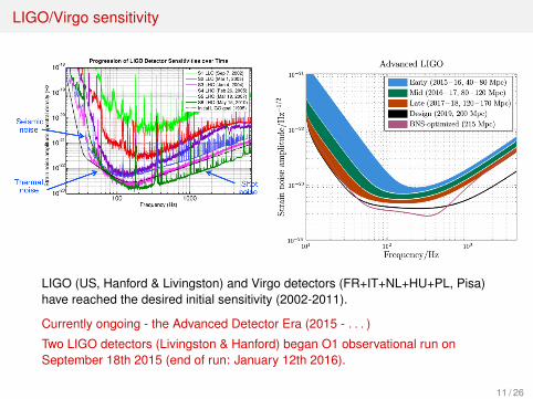
LIGO/Virgo sensitivity

LIGO (US, Hanford & Livingston) and Virgo detectors (FR+IT+NL+HU+PL, Pisa)have reached the desired initial sensitivity (2002-2011).

Currently ongoing - the Advanced Detector Era (2015 - . . . )

Two LIGO detectors (Livingston & Hanford) began O1 observational run onSeptember 18th 2015 (end of run: January 12th 2016).

11 / 26

Advanced Detector Era: 2015 - ...

Sensitivity of AdLIGO and AdVirgo increased by an order of magnitude→distance reach ×10 (sensitivity ∝ 1/r - detection of amplitude, not energy of thewave!)

12 / 26

Neutron stars = very dense, magnetized stars

? The most relativistic, material objects in theUniverse: compactness M/R ' 0.5.

10-2 10-1 100 101

P [s]

10-21

10-20

10-19

10-18

10-17

10-16

10-15

10-14

10-13

10-12

10-11

10-10

10-9

P[s

s−1]

B>Bcrit =4.4 ·10 13 G

Graveyard

104 yr

106 yr

108 yr

10 12 G

10 11 G

10 10 G10 9 G

in binaries

high energymagnetars

other

13 / 26

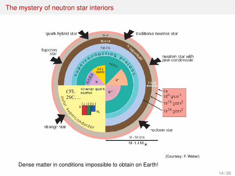
The mystery of neutron star interiors

(Courtesy: F. Weber)

Dense matter in conditions impossible to obtain on Earth!14 / 26

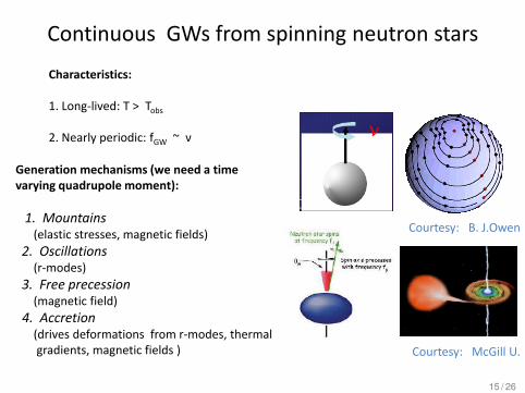
Continuous GWs from spinning neutron stars

v

Characteristics: 1. Long-lived: T > Tobs

2. Nearly periodic: fGW ~ ν

Generation mechanisms (we need a time varying quadrupole moment):

1. Mountains (elastic stresses, magnetic fields)

2. Oscillations (r-modes)

3. Free precession (magnetic field)

4. Accretion (drives deformations from r-modes, thermal gradients, magnetic fields )

Courtesy: B. J.Owen

Courtesy: McGill U.

15 / 26

Example: weak monochromatic signals hidden in the noise

0 200 400 600 800 1000time

4

3

2

1

0

1

2

3

4

h =

n +

s

0.0 0.5 1.0 1.5 2.0 2.5 3.00.0

0.5

1.0

1.5

2.0

2.5

In this case Fourier transform issufficient to detect the signal (a matchedfilter method):

F =

∫ T0

0x(t) exp(−iωt)dt

Signal-to-noise

SNR = h0

√T0

σnoise

16 / 26

In reality: signal is modulated

Since the detector is on Earth, influence of planets and Earth’s rotation changesthe signal’s amplitude and phase.

? Signal is almost monochromatic: pulsars are slowing down,

? To analyze, we have to demodulate the signal (detector is moving),

→ precise ephemerids of the Solar System used.

17 / 26

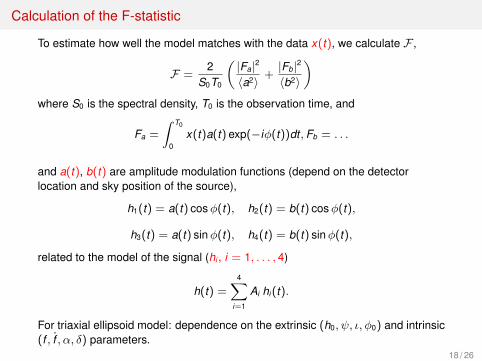
Calculation of the F-statistic

To estimate how well the model matches with the data x(t), we calculate F ,

F =2

S0T0

(|Fa|2

〈a2〉 +|Fb|2

〈b2〉

)where S0 is the spectral density, T0 is the observation time, and

Fa =

∫ T0

0x(t)a(t) exp(−iφ(t))dt,Fb = . . .

and a(t), b(t) are amplitude modulation functions (depend on the detectorlocation and sky position of the source),

h1(t) = a(t) cosφ(t), h2(t) = b(t) cosφ(t),

h3(t) = a(t) sinφ(t), h4(t) = b(t) sinφ(t),

related to the model of the signal (hi , i = 1, . . . , 4)

h(t) =4∑

i=1

Ai hi (t).

For triaxial ellipsoid model: dependence on the extrinsic (h0, ψ, ι, φ0) and intrinsic(f , f , α, δ) parameters.

18 / 26

Methods of data analysis

Computing power ∝ T 50 log(T0). Coherent search of T0 ' 1 yr of data would

require zettaFLOPS (1021 FLOPS)→ currently impossible _

Solution: divide data into shorterlength time frames (T0 ' 2 days)

? narrow frequency bands -sampling time δt = 1/2B,number of data pointsN = T/δt → N = 2TB

→ feasible on a petaFLOPcomputer.

Virgo VSR1 Data (May 18 − Oct 1, 2007)

Fre

quency [H

z]

Time frame number

5 10 15 20 25 30 35 40 45 50 55 60 65100

200

300

400

500

600

700

800

900

Example search space (Virgo Science Run 1).Red: no data, yellow: bad data, green: gooddata.

19 / 26

Typical all-sky search: parameter space

? Narrow (1 Hz) frequency bands f :[100− 1000] Hz,

? Spin-down f1 range proportional tof :

[−1.6× 10−9 f100Hz

, 0] Hz s−1

? All-sky search: number of skypositions α(f ), δ(f ) ∝ f .

Comparison of the f − f plane searched (yellow)with that of other recent all-sky searches:

In our astrophysical applications, the 4-dim parameter space (f , f , α, δ) is big(in VSR1 ' 1017 F-statistic evaluations)

20 / 26

All-sky pipeline

Time domain frame data(Frame library)

Short Fourier TransformData Base (SFDB)(pss sfdb code)

Narrow-band timedomain sequences(ExtractBand &gen2day codes)

Ephemeris data(JPL, LALlibrary)

Grid generation(gridopt code)

Search for candidates(search code)

Search for coincidences(coincidences code)

Followup of promisingcoincidences

(followup code)

? Input data generation (Raw time domain data∼ PB)

? Pre-processing→∼ TB (input time series,detector ephemerids and grid of parameters),

? Stage 1: F-statistic search for candidate GWsignals (the most time-consuming part of thepipeline)

→ 1010 candidates/detector, 100 TB of output.

? Stage 2: Coincidences among candidatesignals from different time segments,

? Stage 3: Followup of interesting coincidences -evaluation of F-statistic along the whole dataspan.

21 / 26

Most expensive part: search for candidate signals

Read data, detector ephemeris& grid generating matrix

Establish sky position

Amplitude andphase demodulation.Resampling (FFT)

Spindown demodulationSkyloop

FFT interpolationSpindown

loop

F-statistics calculation (FFT)

Signals abovethe thresholdregistered

Nextspindown

Sky positionNext skyposition

? Suitable algorithms that allow forFast Fourier Transforms,

? Optimized grid of parameters -minimum number of operation toreach desired sensitivity,

→ partial demodulation before theinner spindown loop (only once persky position),

? Sky positions completelyindepedent of each other

→ ”Embarasingly parallel problem”

22 / 26

First level of parallelization: over the sky positions

30 20 10 0 10 20 30sky position n

15

10

5

0

5

10

15sk

ypos

itio

nm

Sky positions (here in parameter grid coordinates) are independent→Round-robin scheduling.

23 / 26

Second level: massive parallelisation with MPI

Internal MPI scheduling algorithm to run multiple instances of parallel all-skysearch as one massively parallel computation:

? Initialization and estimation ofthe available and necessaryparallel resources,

? Construction of different tasksas groups for requestedfrequencies,

? Size of Group of tasksestimated using frequencyscaling,

? Distribution and decompositionof groups,

? Bookkeeping.

24 / 26

Scheduling and scalability

0 250 500 750 1000 1250 1500 1750 2000 2250 2500frequency [Hz]

48

163264

128256512

1024204840968192

1638432768

para

llel t

asks

per

ban

d

64 128

256

512

1024

2048

4096

8192

1638

4

3276

8

2688

3200

3776

Number of parallel tasks

64

128

256

512

1024

2048

4096

8192

16384

32768

Spee

dup

RealTheory

Amount of computation scaleswell with the band frequency.

SkyFarmer was tested up to 50kCPU tasks.? Scalability is good, but not

optimal:? communication per task

starts to dominate,? suboptimal domain

decomposition due tosimplified scheduling

25 / 26

Current and future plans

? CPU SkyFarmer will be used to analyze the incoming O1 data (40 - 2000Hz, 4 months), using data divided in 2 day segments

→ ' 5× 106 CPU-hours needed,

→ For better sensitivity with 6-day segments, we need ≈ 108 CPU-hours.

? Scaling higher for future exaFLOP computers - hybrid code with GPU.

→ single-GPU code already exists - CUDA cuFFT allowing for considerablespeedup (> 50×).

? Analysing data from future runs: O2, O3,. . . until 2020 and beyond,

? 3 detectors (LIGO + Virgo) or more (+KAGRA, LIGO India...)

26 / 26