anobservingsystemsimulationexperiment(osse)to

Hindawi Publishing CorporationAdvances in MeteorologyVolume 2010, Article ID 743863, 14 pagesdoi:10.1155/2010/743863

Research Article

An Observing System Simulation Experiment (OSSE) toAssess the Impact of Doppler Wind Lidar (DWL) Measurementson the Numerical Simulation of a Tropical Cyclone

Lei Zhang and Zhaoxia Pu

Department of Atmospheric Sciences, University of Utah, 135 S 1460 E, Rm. 819, Salt Lake City, UT 84112, USA

Correspondence should be addressed to Lei Zhang, [email protected]

Received 31 December 2009; Revised 1 April 2010; Accepted 10 April 2010

Academic Editor: Song Y. Hong

Copyright © 2010 L. Zhang and Z. Pu. This is an open access article distributed under the Creative Commons Attribution License,which permits unrestricted use, distribution, and reproduction in any medium, provided the original work is properly cited.

The importance of wind observations has been recognized for many years. However, wind observations—especially three-dimensional global wind measurements—are very limited. A satellite-based Doppler Wind Lidar (DWL) is proposed to measurethree-dimensional wind profiles using remote sensing techniques. Assimilating these observations into a mesoscale model isexpected to improve the performance of the numerical weather prediction (NWP) models. In order to examine the potentialimpact of the DWL three-dimensional wind profile observations on the numerical simulation and prediction of tropical cyclones,a set of observing simulation system experiments (OSSEs) is performed using the advanced research version of the WeatherResearch and Forecasting (WRF) model and its three-dimensional variational (3DVAR) data assimilation system. Results indicatethat assimilating the DWL wind observations into the mesoscale numerical model has significant potential for improving tropicalcyclone track and intensity forecasts.

1. Introduction

Although numerical weather prediction (NWP) models havebeen improved significantly over the past two decades, theforecast accuracy of high-impact weather events, such astropical cyclones, is still a challenging problem in practicalapplications. Since most tropical cyclones occur over tropicaloceans, where conventional observations are sparse, largeuncertainties are presented in the numerical simulationsand predictions due to inaccurate initial conditions. Remotesensing techniques provide an opportunity to observe theatmosphere, especially the atmospheric temperature, mois-ture, and ozone over the oceans either directly or indirectly.However, among all the variables used to represent thestate of the atmosphere, wind measurements are the mostlimited, although the importance of wind observations formeteorological analysis has been recognized for many years[1–3]. Previous studies indicate that wind information playsan important role in improving the tropical and extratrop-ical cyclone forecasts [4–14]. However, the current globalobserving system does not provide a uniform distribution of

tropospheric wind measurements, especially in the tropics,southern hemisphere, and northern hemispheric oceans,where conventional observations are very sparse. During thepast two decades there have been several satellites measuringwind over the oceans, such as the Geosat altimeter, theNational Aeronautics and Space Administration (NASA)Scatterometer (NSCAT), Quick Scatterometer (QuikSCAT),the Special Sensor Microwave Imager (SSM/I), and Euro-pean Space Agency Remote Sensing Satellites (ERS-1/2).QuikSCAT, which was launched in 1999, can provideocean surface wind observations. Some previous studies[15, 16] showed that assimilating QuikSCAT ocean surfacewind observations had a positive impact on improving thenumerical simulation and prediction of tropical cyclones.Other studies also indicated that including SSM/I windinformation had the potential to improve low-level windsimulation [15]. Since SSM/I only provides ocean surfacewind speed measurements, not wind directions, this makesthe viewing of SSM/I winds confusing. NSCAT wind alsoshowed a positive impact on tropical cyclone simulation[10], but NSCAT only provides near-surface wind vectors

2 Advances in Meteorology

over the oceans. Therefore, although wind measurementshave been improved to some extent during the past years,the direct three-dimensional global wind profile measure-ment is still limited. None of the aforementioned satelliteinstruments directly provides wind profile information in thetroposphere.

In recent years, it has been proposed to use Dopplerwind lidar (DWL) to measure the three-dimensional windprofiles either globally, with a polar-orbiting satellite [17],or regionally, if mounted on aircraft [18]. The DWL uses atechnique similar to that of Doppler radars except that a lidaremits pulses of laser light instead of radio waves [18, 19].It is able to measure the wind profile from surface to highaltitudes (e.g., 18 km) with very high vertical resolution. Theobjective of this paper is to examine the potential impact ofDWL measurements from the polar-orbiting satellite on thenumerical simulation and prediction of tropical cyclones.

Generally, the best way to examine the impact of theproposed observations on NWP is to conduct ObservingSystem Simulation Experiments (OSSEs) [20–22]. Thereare several advantages of OSSEs: such as easy control ofthe experiments, precise knowledge of the data propertiesand errors, and knowledge of the truth, and so forth[21]. In this study, the potential impact of the simulatedspace-based DWL three-dimensional (3-D) wind profilemeasurements on the numerical simulation and predictionof tropical cyclone formation and intensification is examinedby conducting a set of OSSEs using the advanced researchversion of the weather research and forecasting (WRF)model and its three-dimensional variational (3DVAR) dataassimilation system.

The advanced research version of the mesoscale com-munity WRF model and its 3DVAR system are brieflydescribed in Section 2. Details of OSSEs setup are presentedin Section 3. The potential impact of assimilating space-based three-dimensional wind profiles on tropical cyclonesimulation and prediction based on OSSE results is examinedin Section 4. Conclusions and discussions about somepractical issues are addressed in Section 5.

2. Numerical Model andData Assimilation System

2.1. The WRF Model. The advanced research versionWRF model (ARW) was developed by the Mesoscale andMicroscale Meteorology (MMM) Division of the NationalCenter for Atmospheric Research (NCAR). The ARW isdesigned to be a flexible, state-of-art atmospheric simu-lation system. This system is suitable for use in a widerange of applications across scales ranging from meters tothousands of kilometers. It is useful for studies of physicalparameterizations, data assimilation, real-time NWP, andso forth. The ARW model is a fully compressible andnon-hydrostatic model with a terrain-following verticalcoordinate. The horizontal grid system is the Arakawa C-grid. The ARW solver uses the Runge-Kutta 2nd and 3rdorder time integration schemes and 2nd and 6th orderadvection schemes in both horizontal and vertical directions.

A small step time-split scheme is used for acoustic andgravity wave modes. A complete description of the WRFmodel can be found in the WRF users guide posted onthe website: http://www.mmm.ucar.edu/wrf/users/docs/. Forthis study, the version 3.0.1 was used in all experiments.

2.2. The WRF 3DVAR System. The WRF 3DVAR assimi-lation system is designed to provide optimal initial andboundary conditions to the WRF model by using variousobservational information sources both from conventionaland nonconventional measurements, such as satellite radi-ance data, radar observations, GPS measurements, and soforth. The WRF 3DVAR is a multivariable data assimilationsystem. The control variables are the stream function,the unbalanced part of potential velocity, the unbalancedpart of temperature, the unbalanced surface pressure, andpseudo relative humidity. The background error correlationis generated using a so-called NMC method [23], which isa popular method for estimating climatological backgrounderror covariances. In the NMC method, the backgrounderrors are approximated by averaging the statistics of thedifferences between two sets of the model forecasts (suchas 24 hr and 12 hr forecasts) valid at the same time. Theobservation errors are assumed to be uncorrelated, so theobservation error covariance matrix is a diagonal matrix. Adetailed description of the 3DVAR system can be found inBarker et al. [24, 25].

3. Experimental Designs

3.1. Case Description. In reality, we do not know the truestate of the atmosphere. In order to quantitatively assess thepotential impact of the proposed observing systems on theNWP models in OSSEs, we need to simulate an atmospherestatus that has the same statistical behavior as that of thereal atmosphere. The simulated “true” atmosphere statusis the so-called nature run (NR). The accuracy of NR isimportant to an OSSE because the OSSE results cannot showthe realistic observational impact on numerical weathersimulation and predictions unless the simulated “true”atmosphere represents most of the characteristics of the realatmosphere.

In order to support community needs in OSSEs, theEuropean Center for Medium-Range Weather Forecasts(ECMWF) produced global nature runs using a spectralprediction model in July 2006 [26]. There are two natureruns with different resolutions: one is at T511 (about 40 kmhorizontal resolution) spectral truncation with 91 verticallevels and 3-hour frequency output from 1200 UTC May 12005 to 0000 UTC June 1 2006. The other one is the higherresolution simulation at T799 (about 25 km horizontalresolution) spectral truncation with 91 vertical levels andhourly output from September 27 2005 to November 1 2005.For simplification, we refer these two global nature runs asT511 NR and T799 NR, respectively. According to the earlyevaluation by Reale et al. [27], the large-scale structure ofthe T511 NR is very realistic. In some cases, smaller scalestructures in the T511 NR are more realistic than in the

Advances in Meteorology 3

10

20

30

40

Nor

th

80 70 60 50 40 30 20

West

(a)

10

20

30

40

Nor

th

80 70 60 50 40 30 20

West

(b)

10

20

30

40

Nor

th

80 70 60 50 40 30 20

West

(c)

10

20

30

40

Nor

th

80 70 60 50 40 30 20

West

(d)

Figure 1: Simulated DWL observation locations at 0600 UTC ((a) and (c)) and 1800 UTC 01 October 2005 ((b) and (d)). (a), (b), (c), and(d) are simulated observation sampling for data assimilation Experiment 1 and Experiment 2, respectively.

reanalysis, which is processed by a much lower resolutionmodel.

Since we intend to evaluate the data impact on tropicalcyclone forecasts with a mesoscale model, we choose to usethe T799 NR. From the T799 NR, a tropical storm, whichoccurred over the Atlantic Ocean during the period from 27September to 11 October 2005, was arbitrarily selected forthis study. The simulation period is from 0600 UTC 01 to0600 UTC 03 October 2005.

3.2. Experimental Design. A two-way nested interactivesimulation was conducted for all experiments. The modelhorizontal resolutions were 27 km for outer domain and9 km for inner domain, respectively. In total there were31 vertical model levels from the surface up to 50 hPa.Various model physics options were used in the differentexperiments.

Four experiments were conducted:

(i) a regional nature run to generate the “truth” field;

(ii) a control run to generate a reference field;

(iii) two data assimilation experiments with differentobservational sampling strategies to investigate thepotential impact of the simulated DWL wind profileson the storm track and intensity forecasts. Resultswere compared against the regional nature run andcontrol run.

Differences in the model setups and configurations for allabove experiments are summarized in Table 1.

3.2.1. Regional Nature Run. In this paper, we mainly focuson the regional numerical model prediction problems. Puet al. [28] has commented that the ECMWF nature runsare sufficiently accurate in describing the tropical cyclonetrack and intensity at an intermediate model resolution.However, they are not good enough in representing thetropical cyclone inner-core structures. Thus, it is necessaryto generate regional nature runs for regional verificationpurposes. In this study, the WRF model was nested inside ofthe ECMWF nature run to generate a set of regional natureruns. The model was initialized using the T799 NR andthen integrated forward for 78 hours starting at 0000 UTC30 September 2005. The domain sizes are 377 × 259 and646 × 583 for the outer and inner domain, respectively. Thehorizontal grid spacing is 27 km for the outer domain and9 km for the inner domain, respectively, as mentioned above.The model physics parameterizations include: the Lin micro-physics scheme, Mellor-Yamada-Janjic planetary boundarylayer model (MYJ), Betts-Miller-Janjic cumulus parameter-ization scheme, RRTM longwave, and Dudhia shortwaveradiation model. Detailed descriptions of each physicalparameterization scheme can be found in Skamarock et al.[29].


Length scale factor = 0.1 850 mb divergence and vector difference

5

10

15

20

25

30

35

40

45

50

Nor

th

80 70 60 50 40 30 20−→20West

−6

−3

−0.5

−0.1

0.1

0.5

3

6

(a)


5

10

15

20

25

30

35

40

45

50

Nor

th

80 70 60 50 40 30 20−→20West

−6

−3

−0.5

−0.1

0.1

0.5

3

6

(b)


5

10

15

20

25

30

35

40

45

50

Nor

th

80 70 60 50 40 30 20−→20West

−6

−3

−0.5

−0.1

0.1

0.5

3

6

(c)


5

10

15

20

25

30

35

40

45

50

Nor

th

80 70 60 50 40 30 20−→20West

−6

−3

−0.5

−0.1

0.1

0.5

3

6

(d)

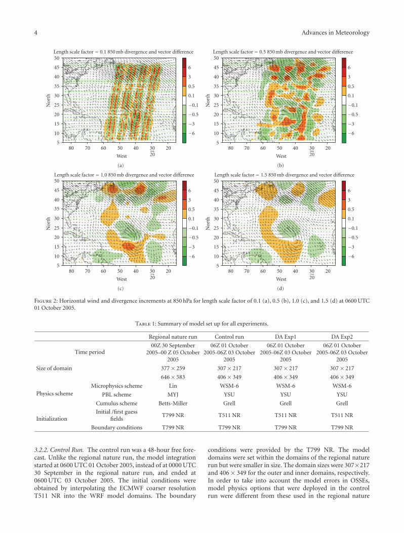
Figure 2: Horizontal wind and divergence increments at 850 hPa for length scale factor of 0.1 (a), 0.5 (b), 1.0 (c), and 1.5 (d) at 0600 UTC01 October 2005.

Table 1: Summary of model set up for all experiments.

Regional nature run Control run DA Exp1 DA Exp2

Time period00Z 30 September

2005–00 Z 05 October2005

06Z 01 October2005-06Z 03 October

2005


2005


2005

Size of domain 377× 259 307× 217 307× 217 307× 217

646× 583 406× 349 406× 349 406× 349

Physics schemeMicrophysics scheme Lin WSM-6 WSM-6 WSM-6

PBL scheme MYJ YSU YSU YSU

Cumulus scheme Betts-Miller Grell Grell Grell

InitializationInitial /first guess

fieldsT799 NR T511 NR T511 NR T511 NR

Boundary conditions T799 NR T799 NR T799 NR T799 NR

3.2.2. Control Run. The control run was a 48-hour free fore-cast. Unlike the regional nature run, the model integrationstarted at 0600 UTC 01 October 2005, instead of at 0000 UTC30 September in the regional nature run, and ended at0600 UTC 03 October 2005. The initial conditions wereobtained by interpolating the ECMWF coarser resolutionT511 NR into the WRF model domains. The boundary

conditions were provided by the T799 NR. The modeldomains were set within the domains of the regional naturerun but were smaller in size. The domain sizes were 307×217and 406× 349 for the outer and inner domains, respectively.In order to take into account the model errors in OSSEs,model physics options that were deployed in the controlrun were different from these used in the regional nature


15

12 15

1518

2124

2730

36

33

30

27

18

129

24 21

15

12

15

2124273033

14

16

18

20

22

24

Nor

th

48 46 44 42 40 38 36 34

West

(a)

15

18

21

24

27

24

21

18

129

6

1518212427

14

16

18

20

22

24

Nor

th

48 46 44 42 40 38 36 34

West

(b)

12

15

24

21

18

27

30

30

159

6

2721

21

24

18

33

1821242730

14

16

18

20

22

24

Nor

th

48 46 44 42 40 38 36 34

West

(c)

18

21

24

27

129

6

18

18

21

24

18

15

18212427

14

16

18

20

22

24

Nor

th

48 46 44 42 40 38 36 34

West

(d)

Figure 3: Horizontal wind structure (wind speed contour and wind vector) at the storm center at 850 hPa from (a) regional nature run, (b)control run, (c) data assimilation Experiment 1, and (d) data assimilation Experiment 2 at 0600 UTC 01 October 2005. The contour intervalof wind speed is 3 m s−1, the areas with wind speed exceeding 20 m s−1 are shaded.

run. Thus, the physics options include: the WRF Single-Moment 6-class microphysics scheme (WSM-6), the YonseiUniversity planetary boundary layer model (YSU PBL),and the Grell-Devenyi ensemble cumulus parameterizationscheme. Other parameters are same as in the regional naturerun.

3.2.3. Simulation of Observations. According to Marseilleet al. [12, 13], the DWL was assumed to be aboard ona given polar-orbiting satellite. This means that the windmeasurements are available only twice daily over the sameregion. An idealized distribution of observations is used

following an early suggestion from D. Emmitt (personalcommunication). Considering the influence of clouds, twoconfigurations of the observations sampling are simulated.Figures 1(a) and 1(b) show the distributions of the simulatedDWL observations in data assimilation Experiment 1 (DAExp1) at 0600 UTC and 1800 UTC 01 October 2005, respec-tively. In this observational configuration, cloud effect is nottaken into account. Wind observations are available fromnear the surface up to 18 km. To simulate the DWL samplingin cloudy atmospheres, we used the realistic atmosphericconditions extracted from the regional nature run dataset.Figures 1(c) and 1(d) represent the simulated observation


14

16

18

20

22

24

26

Nor

th

50 48 46 44 42 40 38 36 34

West

3

6

9

12

15

18

21

24

27

30

(a)

14

16

18

20

22

24

26

Nor

th

50 48 46 44 42 40 38 36 34

West

3

6

9

12

15

18

21

24

27

30

(b)

14

16

18

20

22

24

26

Nor

th

50 48 46 44 42 40 38 36 34

West

3

6

9

12

15

18

21

24

27

30

(c)

14

16

18

20

22

24

26

Nor

th

50 48 46 44 42 40 38 36 34

West

3

6

9

12

15

18

21

24

27

30

(d)

Figure 4: The wind shear (units: m s−1) between 850 hPa and 200 hPa at 0600 UTC 01 October 2005 from (a) regional nature run, (b) controlrun, (c) data assimilation Experiment 1, and (d) data assimilation Experiment 2.

configurations with consideration of the cloud effect and areused in data assimilation Experiment 2 (DA Exp2). Sincethe cloud effect is taken into account in this case, windprofiles are not available in areas with cloud contamination.In both DA Exp1 and DA Exp2, the observations used fordata assimilation experiments are generated by interpolatingthe “truth” field (regional nature run) both horizontally andvertically from the model grids onto the simulated observa-tional locations and by superimposing random noises. Thevertical resolution of the measurements is 250 m below and1 km above the 2 km level. Typical values for the standarddeviation of DWL wind errors are 2 m s−1below 2 km and3 m s−1 above the 2 km level [30]. No bias has been assumedfor the simulated DWL wind errors.

3.2.4. Data Assimilation Experiments. The WRF 3DVARsystem was used to assimilate DWL wind profiles. Cor-responding to the two configurations of the simulated

observations mentioned in Section 3.2.3, two data assim-ilation experiments are performed: the first is an idealexperiment that does not consider cloud influence. Theobservational samplings are shown in Figures 1(a) and 1(b)for 0600 UTC and 1800 UTC, respectively. For simplification,in this paper it is referred as DA Exp1. The other oneis a more realistic experiment. As shown in Figures 1(c)(for 0600 UTC) and 1(d) (for 1800 UTC), the observationscontaminated by clouds are eliminated. For simplification itis referred as DA Exp2. Similar to the control run, the modeldomain configuration and physics options for both of thesetwo experiments are the same as those used in the controlrun. The first guess field was initialized at 0600 UTC 01October 2005 from the T511 NR. A cycled data assimilationwas carried out to assimilate simulated DWL wind profilesbetween 0600 UTC and 1800 UTC 01 October 2005. The dataassimilation was conducted between 0600 UTC 01 October2005 and 1800 UTC 01 October 2005. After that, the model


1000

900

800

700

600

500

400

300

200

100P

ress

ure

(hPa

)

−3 −2 −1 0 1 2 3

Averaged divergence (1e − 5 s−1)

Regional NRControl

DA Exp 1DA EXP 2

Figure 5: Area-averaged divergence vertical profiles over the areawith radius of 250 km around the storm center at 0600 UTC 01October 2005 (black line: regional nature run; blue line: controlrun; red line: data assimilation Experiment 1; green line: dataassimilation Experiment 2).

initial condition was replaced by the analysis from dataassimilation experiments and then a 36-hour forecast wasconducted from 1800 UTC 01 October to 0600 UTC 03October 2005. All results presented in this paper use theresults from the 9 km grid domain.

4. Results and Discussion

4.1. Sensitivity of DWL Data Assimilation to Background ErrorCorrelations. The basic goal of the 3DVAR is to find anoptimal estimate of the model initial conditions at analysistime through the minimization of a cost function J:

J = Jb + Jo, (1)

Jb = 12

(x − xb)TB−1(x − xb), (2)

Jo = 12

(H(x)− yo

)TO−1(H(x)− yo). (3)

The cost function J is a combination of a backgroundterm Jb and an observation term Jo (1). Here Jb is the back-ground term that measures the distance between analysis andbackground (2), Jo is the observation term that measures thedistance between observations and model-simulated obser-vations (3). The superscripts −1 and T denote the inverseand adjoint of a matrix or a linear operator, respectively. B isthe background error covariance matrix. In this study, the B

16

18

20

22

24

Nor

th

48 46 44 42 40

West

Regional NRControl

DA Exp 1DA EXP 2

(a)

0

50

100

150

200

250

300Tr

ack

erro

r(k

m)

0 6 12 18 24 30 36 42 48

Forecast hours

DA Exp 2DA EXP 1Control

(b)

Figure 6: Time series of the tropical cyclone (a) track and (b)track error during 48-hour simulations for different experiments(black line: regional nature run; blue line: control run; red line: dataassimilation Experiment 1; green line: data assimilation Experiment2) from 0600 UTC 01 to 0600 UTC 03 October 2005.

matrix was generated using the NMC-method [23], which isa popular method used for background error estimation. O isthe observation error covariance matrix. xb is the first guessfield, usually it is a short-range forecast or from an analysis. His the observation operator that transforms model variablesfrom model physical space to the observation space. yo is theobservation at the analysis time.

The background error covariance matrix (B matrix) playsan important role in a 3DVAR system. It influences theanalysis fit to observations and also define the influencingdistance of the analysis response from the observations. Inthe horizontal direction, the background error correlationsare assumed to be a Gaussian probability density func-tion (4). The observational information is spread using a


980

985

990

995

1000

Min

imu

mse

ale

velp

ress

ure

(hPa

)

0 6 12 18 24 30 36 42 48

Forecast hours (h)

Regional NRControl

DA Exp 1DA EXP 2

(a)

22

24

26

28

30

32

34

Max

imu

msu

rfac

ew

ind

spee

d(m

/s)

0 6 12 18 24 30 36 42 48

Forecast hours (h)

Regional NRControl

DA Exp 1DA EXP 2

(b)

Figure 7: Time series of (a) minimum Sea Level Pressure (SLP)at the storm center and (b) maximum surface wind speed fromdifferent experiments (black line: regional nature run; blue line:control run; red line: data assimilation Experiment 1; green line:data assimilation Experiment 2) from 0600 UTC 01 to 0600 UTC 03October 2005.

recursive filter, while the vertical relation is represented byapplying the empirical orthogonal decomposition technique:

B(r) = B(0) exp

(

− r2

s2

)

. (4)

In (4), r is the distance between the model grid pointand the observation location, s is the length scale of theGaussian function, and it determines how far the observationinformation can be spread spatially. B(0) is the backgroundcovariance at observation location and B(r) is the back-ground error covariance at the model grid point away fromthe observation location with distance r.

Since the B matrix is based on climatological statistics, inorder to specify it for the DWL data and grid resolution usedin this particular study, four experiments were conducted toexamine the impact of different length scales on the analysisresults of wind fields where the length scales were set to0.1, 0.5 1.0, and 1.5 times of the original values (which usesstatistics from the NMC method). The data assimilated in

all of these four experiments are the DWL wind profilesfrom Figure 1(a). Figure 2 shows the horizontal wind vectorsand divergence increments (i.e., 3DVAR analysis minus firstguess) from these four experiments at 850 hPa at analysistime 0600 UTC 01 October 2005. It shows that the horizontaldistributions of the analysis increments from assimilationof DWL data were significantly different among these fourexperiments. If a small length scale (such as 0.1 times of theoriginal values) was used, the observations only influencedthe areas surrounding its locations. This implies that, inthis situation, the observation information cannot be usedoptimally and that areas far away from the observationlocations cannot benefit from the observations. If a largelength scale (such as 1.5 times of the original values) wasemployed, although the observation information was spreadto the areas far away from the observation locations, therelations were not always realistic for practical applica-tions. Therefore, in practical applications, determining areasonable horizontal correlation length scale for variouskinds of observations, model resolutions, and observationdensity is still a challengeable question for a 3DVAR method.Comparing the analysis results from all four experiments, alength scale of 1.0 seems to be optimal for the analysis of theDWL data in this study. Therefore, a length scale factor of 1.0was adapted for all experiments.

4.2. Data Impact on Initial Conditions

4.2.1. Horizontal Wind Structures. Figure 3 shows the hor-izontal winds at 850 hPa from the regional nature run, thecontrol run, DA Exp1, and DA Exp2 at 0600 UTC 01 October2005, respectively. In Figure 3, the shaded areas indicateregions with wind speed exceeding 20 m s−1. Compared withthe regional nature run simulation, both the control runand data assimilation experiments are able to reproducethe basic structures of the storm wind field. However, thesimulated wind speed from the control run was weakerthan that from the data assimilation experiments. After dataassimilation, a more intensive wind structure was found nearthe storm center. In DA Exp1, the wind field in the southeastof the storm center was strengthened and the location ofthe regions with wind speed exceeding 20 m s−1 agreed wellwith the regional nature simulation. The maximum surfacewind speed near the storm center reached 26.3 m s−1. Thisindicates that assimilation of DWL wind profiles enhancedthe wind field around storm center. In DA Exp2, the windfield around the storm center was not enhanced as in DAExp1. This could be mainly attributed to the fact that thereare fewer observations available over the storm center in DAExp2.

4.2.2. Wind Shear. Wind shear, which is the change inwind speed or direction with height in the atmosphere, isone of the most critical factors controlling tropical cycloneformation and destruction [31]. Figure 4 illustrate the windshear between 850 hPa and 200 hPa at 0600 UTC 01 October2005 from the regional nature run, the control run, DAExp1 and DA Exp2, respectively. The wind shear structures


20

20 20

20

25

25

20

20

30

35

25

35

35

10

40

40

4010

2025

2515

30

1510

15

1515

15

20303540

18

20

22

24

26N

orth

50 48 46 44 42 40 38

West

(a)

15

5

2535

10

25

25

25

15

10

20

20

20

30

2030

20

30

20

1525

18

20

22

24

26

Nor

th

50 48 46 44 42 40 38

West

(b)

10

20

4020

155

1510

20253035

25

25

15

15

20

35

40

40

30

2530

35

3025

1515

18

20

22

24

26

Nor

th

50 48 46 44 42 40 38

West

(c)

2025

20

30

25

25

10

15

10

20

30

35

15 10

35

40

25

15

20

3035

18

20

22

24

26N

orth

50 48 46 44 42 40 38

West

(d)

Figure 8: Same as Figure 3 but at 1800 UTC 02 October 2005. The contour interval of wind speed is 5 m s−1, the areas with wind speedexceeding 26 m s−1 are shaded.

were well reproduced after assimilating DWL wind profilesas simulated structural features was much closer to that ofthe regional nature run. In both the control run and dataassimilation experiments, the simulated maximum windshear appears in the north of the storm center. It is a littlefarther to the west compared to the regional nature run.But in the control run, in the south of the storm centerthe wind shear from the control run was weaker than thosefrom DA Exp1 and DA Exp2. This indicates that assimilationof 3D wind profiles has the potential to adjust the verticalstructures of the wind field to some extent. In addition, sincethe observations over the storm center were available andwere assimilated in DA Exp1, the structure of the wind sheararound the storm center is much closer to that of the regionalnature run, compared with the DA Exp2 analysis results.

4.2.3. Divergence Fields. Figure 5 shows the area-averageddivergence vertical profiles within a radius of 250 km aroundthe storm center for these four experiments at 0600 UTC01 October 2005. Compared to the results from the dataassimilation experiments, in the control run, the divergencevariation with height showed a larger difference fromthe regional nature run simulation. For data assimilationexperiments, in DA Exp1, from the surface to 400 hPa,the area-averaged divergence was very close to that of theregional nature run; above 400 hPa, the divergence profile didnot keep close to the nature run simulations. But, it kept thesame tendency. DA Exp2 did not behave as good as DA Exp1,but it still performed better than the control run. A possibleexplanation for this is the fact that more observations overthe storm center were included in DA Exp1.


14

16

18

20

22

24

26

28

30N

orth

54 51 48 45 42 39 36 33

West

100

200

250

300

350

400

450

475

500

525

550

575

600

(a)

14

16

18

20

22

24

26

28

30

Nor

th

54 51 48 45 42 39 36 33

West

100

200

250

300

350

400

450

475

500

525

550

575

600

(b)

14

16

18

20

22

24

26

28

30

Nor

th

54 51 48 45 42 39 36 33

West

100

200

250

300

350

400

450

475

500

525

550

575

600

(c)

14

16

18

20

22

24

26

28

30

Nor

th

54 51 48 45 42 39 36 33

West

100

200

250

300

350

400

450

475

500

525

550

575

600

(d)

Figure 9: The surface latent heat flux (W m−1) from (a) regional nature run, (b) control run, (c) data assimilation Experiment 1, and (d)data assimilation Experiment 2 at 1800 UTC 02 October 2005.

4.3. Impact on Forecasts

4.3.1. Track and Intensity. Figures 6 and 7 show the timeevolution of the simulated track and minimum central sealevel pressure (SLP) and maximum surface wind speed fordifferent experiments.

From Figure 6, the simulated storm track in the con-trol run was farther to the west and the storm movedslightly quicker compared to the regional nature run. Afterassimilating the DWL 3D wind profiles, the storm trackforecast was improved and the predicted storm track errorwas reduced compared to the control run. Compared withthe results from DA Exp2, the simulated storm track inDA Exp 1 is much closer to the nature run simulations(“truth”) in the first 24-h simulation. The track errors aresmaller than those from DA Exp2. The advantages from DAExp1 can be attributed to including the observations overcloudy areas (most of them over the storm center). After 36

hours simulation, the DA Exp2 performed better in tracksimulation.

In the regional nature run (“truth”), the minimumcentral SLP was 991 hPa and steadily dropped to 983 hPawithin the first 36-hour simulation. It then deepened slowlyduring the following 12 hours (Figure 7). Accordingly, themaximum surface wind intensified gradually in the first 36hours and then increased slowly in the following 12 hours.The simulated minimum central SLP of the storm from thecontrol run showed the same tendency during the 48-hoursimulation but it was weaker than that from the regionalnature run. The maximum surface wind was also weakerthan that from the regional nature run. In DA Exp1, boththe minimum SLP and the maximum surface wind wereimproved significantly during the first 36 hours, and thenthe improvements decreased slightly over the next 12 hours.In DA Exp2, the storm intensity was also improved after


16

18

20

22

24

Nor

th

50 48 46 44 42 40 38

West

0.1

0.2

0.4

0.8

1.6

3.2

6.4

12.8

25.6

51.6

(a)

16

18

20

22

24

Nor

th

50 48 46 44 42 40 38

West

0.1

0.2

0.4

0.8

1.6

3.2

6.4

12.8

25.6

51.6

(b)

16

18

20

22

24

Nor

th

50 48 46 44 42 40 38

West

0.1

0.2

0.4

0.8

1.6

3.2

6.4

12.8

25.6

51.6

(c)

16

18

20

22

24N

orth

50 48 46 44 42 40 38

West

0.1

0.2

0.4

0.8

1.6

3.2

6.4

12.8

25.6

51.6

(d)

Figure 10: The simulated accumulated 3 hours rainfall (mm) from (a) regional nature run, (b) control run, (c) data assimilation Experiment1, and (d) data assimilation Experiment 2 at 1800 UTC 02 October 2005.

data assimilation, but the improvements were a little weakercompared to that of DA Exp1.

In order to further examine the impact of DWL data onthe simulation and prediction of tropical cyclones, diagnoseswere also conducted for several other parameters as follows.

4.3.2. Horizontal Wind Structures. As discussed in Sec-tion 4.2.1, assimilation of DWL wind profiles enhanced thewind field at the initial time. It also made improvements inthe wind simulations during the following forecast period.Figure 8 is the same as Figure 3 but for 1800 UTC 02 October2005 (36 hours forecast). The shaded areas indicate theregions with wind speed exceeding 26 m s−1. Although boththe control run and data assimilation experiments are able toproduce the basic structure of the horizontal wind field, thesimulated locations of the storm center are different. In thecontrol run, the simulated storm center was farther to the

west compared with the regional nature run simulation. Inthe data assimilation experiments (DA Exp1 and DA Exp2),the simulated storm centers are much closer to these fromthe regional nature run. In addition, the simulated wind fieldin the control run was much weaker than those from thedata assimilation experiments. Compared with the regionalnature run simulation, the horizontal wind intensity wasbetter represented after data assimilation.

4.3.3. Surface Latent Heat Fluxes. Surface latent heat flux isthe flux of heat from the Earth’s surface to the atmospherethat is, associated with evaporation or transportation ofwater from the surface and subsequent condensation ofwater vapor in the troposphere. The heating at low-levelsfrom the surface can substantially modify the temperaturefield thereby enhancing or destroying the baroclinic envi-ronment. In addition, the latent heat release, derived from


1.5

2

2.5

3

3.5

4

4.5

5

Rai

nra

te(m

m/h

r)

6 12 18 24 30 36 42 48

Forecast hours

Regional NRControl

DA Exp 1DA EXP 2

Figure 11: The time series of area-averaged rain rate (mm/hr) overthe area with radius of 250 km around the storm center between1200 UTC 01 and 0600 UTC 03 October 2005. (Black line: regionalnature run; blue line: control run; red line: data assimilationExperiment 1; green line: data assimilation Experiment 2).

condensation throughout the troposphere can also be acrucial factor determining the vertical extent of the intensedeepening of tropical cyclones. The influence of the latentheat flux over oceanic cyclones has been studied in manyprevious studies [32–36]. It was shown that the latent heatflux plays an important role in hurricane formation andintensification [15]. The study by Papasimakis et al. [37]indicates that hurricane development is heavily related tolatent heat release. It was also pointed out that latent heatrelease had positive impacts on hurricane development andintensification. Figure 9 show the latent heat flux from thesefour experiments at 1800 UTC 02 October 2005. In theregional nature run (Figure 9(a)), the maximum latent heatrelease occurred mainly in the northeast of the storm center,while the simulated latent heat flux was too weak in thecontrol run (Figure 9(b)). The locations of maximum latentheat flux in the data assimilation experiments are farther tothe west of these from the regional nature run simulation;but the assimilations of the DWL wind profiles (Figures 9(c)and 9(d)) produced a larger latent heat flux around the stormcenter that was helpful for storm development. As a result,the wind field was strengthened in the simulations with dataassimilation.

4.3.4. Rainfall Simulation. Figure 10 compare the accu-mulated 3-hour precipitation around the storm center at1800 UTC 02 October 2005. It shows that the precipitationnear the region of 22N and 43W (northeast of the stormcenter) was well simulated in the experiments with dataassimilation (DA Exp 1 and 2), compared to the controlrun results. Both the simulated quantity and location ofthe maximum rainfall are similar to the regional naturerun. For the control run simulation, the simulated rainfallsurrounding the storm center is relatively weak compared tothe regional nature run.

To further examine the impact of the assimilation ofDWL wind profiles on precipitation forecasts, the area-averaged, storm-induced rainfall rates from different exper-iments were compared. Figure 11 illustrates the time series

of the rainfall rate averaged in the region within a radiusof 250 km from the storm center in different experimentscompared with the results from the regional nature runbetween 1200 UTC 01 and 0600 UTC 03 October 2005. Asshown in the figure, both the control run and the dataassimilation experiments underestimated the rainfall rateas produced in the regional nature run. However, the dataassimilation experiments (DA Exp1 and DA Exp2) improvedthe rainfall forecasts in the first 36 hours, although they didnot perform well in the last 12 hours of the simulations.

5. Summary and Discussions

The potential impact of simulated Doppler Wind Lidar(DWL) wind profiles on the numerical simulation andprediction of tropical cyclones has been investigated usingthe WRF model and its 3DVAR data assimilation systemby means of Observing System Simulation Experiments(OSSEs). Results indicated that, for this particular case, theassimilation of DWL wind profiles had the potential toimprove both the horizontal and vertical wind structuresand hence we could simulate stronger wind circulation. Thesimulated storm track and intensity were also improvedafter assimilation of DWL wind profiles during the 48-hour simulation. Results from the two data assimilationexperiments with different observation sampling strategieshave shown that assimilating the wind observations aroundthe storm center is useful for improving storm track andintensity simulations.

Future studies will be performed to evaluate the DWLwind observation impact with different sampling strategies,such as different horizontal and vertical resolutions of themeasurements. A more comprehensive evaluation of theimpacts of the DWL data on operational tropical cycloneforecasts will also be assessed using operational models andintegrating the DWL data with all other conventional andsatellite data available.

Acknowledgments

The computer time for this study was provided by NASAHigh-End Computing System and the Center for HighPerformance Computing (CHPC) at the University of Utah.Authors are grateful to Drs. Lars Peter Riishojggard andMichiko Masutani for providing ECMWF nature run datathrough a joint OSSE effort. The second author would like tothank Drs. G. David Emmitt, Bruce Gentry and Robert Atlasfor useful discussion. This study is supported by NASA Grantno. NNX08AH88G.

References

[1] W. E. Baker, G. D. Emmitt, F. Robertson, et al., “Lidar-measured winds from space: a key component for weather andclimate prediction,” Bulletin of the American MeteorologicalSociety, vol. 76, no. 6, pp. 869–888, 1995.

[2] W. A. Lahoz, R. Brugge, D. R. Jackson, et al., “An observingsystem simulation experiment to evaluate the scientific meritof wind and ozone measurements from the future SWIFT


instrument,” Quarterly Journal of the Royal MeteorologicalSociety, vol. 131, no. 606, pp. 503–523, 2005.

[3] A. Stoffelen, J. Pailleux, E. Kallen, et al., “The atmosphericdynamics mission for global wind field measurement,” Bul-letin of the American Meteorological Society, vol. 86, no. 1, pp.73–87, 2005.

[4] C. S. Velden, T. L. Olander, and S. Wanzong, “The impact ofmultispectral GOES-8 wind information on Atlantic tropicalcyclone track forecasts in 1995. Part I: dataset methodology,description, and case analysis,” Monthly Weather Review, vol.126, no. 5, pp. 1202–1218, 1998.

[5] J. S. Goerss, C. S. Velden, and J. D. Hawkins, “The impact ofmultispectral GOES-8 wind information on Atlantic tropicalcyclone track forecasts in 1995. Part II: NOGAPS forecasts,”Monthly Weather Review, vol. 126, no. 5, pp. 1219–1227, 1998.

[6] I. Szunyogh, Z. Toth, R. E. Morss, S. J. Majumdar, B. J.Etherton, and C. H. Bishop, “The effect of targeted dropsondeobservations during the 1999 Winter Storm ReconnaissanceProgram,” Monthly Weather Review, vol. 128, no. 10, pp. 3520–3537, 2000.

[7] P. M. Boorman, R. Swinbank, and D. A. Ortland, “Assimilationof directly measured stratospheric winds into the UnifiedModel,” Forecasting Research Technical Report 332, MetOffice, 2000.

[8] L. Isaksen and A. Stoffelen, “ERS scatterometer wind dataimpact on ECMWF’s tropical cyclone forecasts,” IEEE Trans-actions on Geoscience and Remote Sensing, vol. 38, no. 4, pp.1885–1892, 2000.

[9] L. Isaksen and P. A. E. M. Janssen, “Impact of ERS scatterome-ter winds in ECMWF’s assimilation system,” Quarterly Journalof the Royal Meteorological Society, vol. 130, no. 600, pp. 1793–1814, 2004.

[10] S. M. Leidner, L. Isaksen, and R. N. Hoffman, “Impact ofNSCAT winds on tropical cyclones in the ECMWF 4DVARassimilation system,” Monthly Weather Review, vol. 131, no. 1,pp. 3–26, 2003.

[11] N. Zagar, “Assimilation of equatorial waves by line-of-sightwind observations,” Journal of the Atmospheric Sciences, vol.61, no. 15, pp. 1877–1893, 2004.

[12] G. J. Marseille and A. Stoffelen, “Simulation of wind profilesfrom a space-borne Doppler wind lidar,” Quarterly Journal ofthe Royal Meteorological Society, vol. 129, no. 594, pp. 3079–3098, 2003.

[13] G.-J. Marseille, A. D. Stoffelen, and J. A. N. Barkmeijer,“Impact assessment of prospective spaceborne Doppler windlidar observation scenarios,” Tellus A, vol. 60, no. 2, pp. 234–248, 2008.

[14] G.-J. Marseille, A. D. Stoffelen, and J. Barkmeijer, “A cycledsensitivity observing system experiment on simulated Dopplerwind lidar data during the 1999 Christmas storm “Martin”,”Tellus A, vol. 60, no. 2, pp. 249–260, 2008.

[15] S.-H. Chen, “The impact of assimilating SSM/I and QuikSCATsatellite winds on Hurricane Isidore simulations,” MonthlyWeather Review, vol. 135, no. 2, pp. 549–566, 2007.

[16] Z. Pu, X. Li, C. Velden, S. Aberson, and W. T. Liu, “Impact ofaircraft dropsonde and usatellite wind data on the numericalsimulation of two landfalling tropical storms during TCSP,”Weather and Forecasting, vol. 23, pp. 62–79, 2008.

[17] D. G. H. Tan and E. Andersson, “Simulation of the yield andaccuracy of wind profile measurements from the AtmosphericDynamics Mission (ADM-Aeolus),” Quarterly Journal of theRoyal Meteorological Society, vol. 131, no. 608, pp. 1737–1757,2005.

[18] M. Weissmann and C. Cardinali, “Impact of airborne Dopplerlidar observations on ECMWF forecasts,” Quarterly Journal ofthe Royal Meteorological Society, vol. 133, no. 622, pp. 107–116,2007.

[19] C. J. Grund, R. M. Banta, J. L. George, et al., “High-resolutiondoppler lidar for boundary layer and cloud research,” Journalof Atmospheric and Oceanic Technology, vol. 18, no. 3, pp. 376–393, 2001.

[20] C. P. Arnold Jr. and C. H. Dey, “Observing-systems simulationexperiments: past, present and future,” Bulletin of the Ameri-can Meteorological Society, vol. 67, no. 6, pp. 687–695, 1986.

[21] R. M. Atlas, “Observing system simulation experiments:methodology, examples and limitations,” in CGC/WMOWorkshop, Geneva, Switzerland, April 1997, WMO TD No.868.

[22] S. J. Lord, E. Kalnay, R. Daley, G. D. Emmitt, and R. Atlas,“Using OSSEs in the design of future generation integratedobserving systems,,” in Proceedings of the 1st Symposium onIntegrated Observing Systems, pp. 45–47, AMS, Long Beach,Calif, USA, 1997, preprints.

[23] D. F. Parrish and J. C. Derber, “The National MeteorologicalCenter’s spectral statistical-interpolation analysis system,”Monthly Weather Review, vol. 120, no. 8, pp. 1747–1763, 1992.

[24] D. M. Barker, W. Huang, Y.-R. Guo, A. J. Bourgeois, and Q.N. Xiao, “A three-dimensional variational data assimilationsystem for MM5: implementation and initial results,” MonthlyWeather Review, vol. 132, no. 4, pp. 897–914, 2004.

[25] D. M. Barker, M. S. Lee, Y.-R. Guo, W. Huang, Q.-N. Xiao,and R. Rizvi, “WRF variational data assimilation developmentat NCAR,” in Proceedings of the 5th WRF/14th MM5 Users’Workshop, p. 5, NCAR, Boulder, Colo, USA, 2004.

[26] M. Masutani, J. S. Woollen, S. J. Lord, et al., “Observingsystem simulation experiments at the National Centers forEnvironmental Prediction,” Journal of Geophysical Research D,vol. 115, no. 7, Article ID D07101, 2010.

[27] O. Reale, J. Terry, M. Masutani, E. Andersson, L. P. Riisho-jgaard, and J. C. Jusem, “Preliminary evaluation of theEuropean Centre for Medium-Range Weather Forecasts’(ECMWF) Nature Run over the tropical Atlantic and Africanmonsoon region,” Geophysical Research Letters, vol. 34, no. 22,Article ID L22810, 6 pages, 2007.

[28] Z. Pu, L. Zhang, B. Gentry, and B. Demoz, “Potential impact oflidar wind measurements on high-impact weather forecasting:a regional OSSEs study,” in Proceedings of the 13th AMSConference on Integrated Observing Systems for Atmosphere,Ocean, and Land Surface (IOAS-AOLS ’09), Phoenix, Ariz,USA, January 2009.

[29] W. C. Skamarock, J. B. Klemp, J. Dudhia, et al., “A descriptionof the advanced research WRF version 2,” NCAR TechnicalNote NCAR/TN-468+STR, NCAR, Boulder, Colo, USA, 2005.

[30] W. Baker, “Concept for a US space-based wind lidar: status andcurrent activities,” in Joint Center for Satellite Data Assimilation(JCSDA) Seminar, July 2009.

[31] W. M. Frank and E. A. Ritchie, “Effects of vertical windshear on the intensity and structure of numerically simulatedhurricanes,” Monthly Weather Review, vol. 129, no. 9, pp.2249–2269, 2001.

[32] W. A. Nuss and R. A. Anthes, “A numerical investigation oflow-level processes in rapid cyclogenesis,” Monthly WeatherReview, vol. 115, pp. 2728–2743, 1987.

[33] E. Rogers and L. F. Bosart, “A diagnostic study of two intenseoceanic cyclones,” Monthly Weather Review, vol. 119, no. 4, pp.965–996, 1991.


[34] G. H. Crescenti and R. A. Weller, “Analysis of surface fluxesin the marine atmospheric boundary layer in the vicinity ofrapidly intensifying cyclones,” Journal of Applied Meteorology,vol. 31, no. 8, pp. 831–848, 1992.

[35] P. J. Neiman and M. A. Shapiro, “The life cycle of anextratropical marine cyclone. Part I: frontal-cyclone evolutionand thermodynamic air-sea interaction,” Monthly WeatherReview, vol. 121, no. 8, pp. 2153–2176, 1993.

[36] D.-L. Zhang, E. Radeva, and J. Gyakum, “A family of frontalcyclones over the western Atlantic Ocean. Part II: parameterstudies,” Monthly Weather Review, vol. 127, no. 8, pp. 1745–1760, 1999.

[37] N. Papasimakis, G. Cervone, F. Pallikari, and M. Kafatos,“Multifractal character of surface latent heat flux,” Physics A,vol. 372, no. 2, pp. 703–718, 2006.

anobservingsystemsimulationexperiment(osse)to

Documents