anurag college of engineering (anrh)
TRANSCRIPT

ANURAG COLLEGE OF ENGINEERING (ANRH)
Aushapur(V), Ghatkesar(M), Medchal(Dist)- 501301
DEPARTMENT OF BASIC SCIENCES AND HUMANITIES
PH105BS : ENGINEERING PHYSICS LAB B.Tech. I Year I Sem
( Common for Civil, ME, AE, ME (M), MME, Mining & Petroleum Engg.)
List of Experiments:-
1. Melde’s experiment: To determine the frequency of a vibrating bar or turning fork using
Melde’s arrangement.
2. Torsional pendulum: To determine the rigidity modulus of the material of the given wire using
torsional pendulum.
3. Newton’s rings: To determine the radius of curvature of the lens by forming Newton’s rings.
4. Diffraction grating: To determine the number of lines per inch of the grating.
5. Dispersive power: To determine the dispersive power of prism by using spectrometer.
6. Coupled Oscillator: To determine the spring constant by single coupled oscillator.
7 .LCR Circuit: To determine quality factor and resonant frequency of LCR circuit.
8 LASER: To study the characteristics of LASER sources.
9. Optical fiber: To determine the bending losses of Optical fibers.
10. Optical fiber: To determine the Numerical aperture of a given fiber.

Fig :- A standing wave is created when an incident and reflected wave have identical amplitudes,
wavelengths and velocities.
Fig :- Transverse arrangement
Fig :- Longitudinal arrangement

MELDE’S EXPERIMENT-Transvers and Longitudinal Modes
AIM: -To determine the frequency of a vibrating bar of tuning fork using Melde’s arrangement in
transverse and longitudinal modes.
APPARATUS: -Smooth pulley fixed to a stand, tuning fork, Connecting wires, Weight box, Pan, Thread & Battery eliminator.
THEORY: -When a vibrating body produces waves along a tightly stretched string, the waves are reflected
at the end of the string, which cause two opposite traveling waves to exist on the string at the same time.
These two waves interfere with each other, creating both constructive and destructive interference in the
vibrating string. If the two waves have identical amplitudes, wavelengths and velocities, a standing wave or
stationary wave is created.
The constructive and destructive interference patterns caused by the superposition of the two waves
create points of minimum displacement called nodes, or nodal positions, and points of maximum
displacement called antinodes. If we define the distance between two nodes (or between two antinodes)
to be , then the wavelength of the standing wave is . Figure illustrates the case where the length
of string vibrates with 5 nodes and 4 antinodes. On the basis of the direction of movement of the individual
particles of the medium relative to the direction that the waves travel in Transverse and Longitudinal
modes.
a) Transverse arrangement: In this arrangement, a wave in which particles of the medium moves in a
direction, perpendicular to the direction of the propagation. The fork is placed in the transverse vibration
position and by adjusting the length of the string and weights in the pan, the s tr i ng starts vibrating &
f o rm s many wel l -defined l oops . The time, during which the tuning fork completes one vibration, the
string also completes one vibration. In this mode, frequency of the string is equal to the frequency of the
tuning fork.
b) Longitudinal arrangement: In this arrangement a wave in which particles of the medium move in a
direction parallel to the direction of the propagation. When the fork is placed in the longitudinal position
and the string makes longitudinal vibrations, The time, during which the tuning fork completes one
vibration, the string completes half of its vibration. In this mode, frequency of the fork is twice the frequency of the string. In longitudinal drive mode, since the string tension increases and decreases once per tuning
fork vibration, it takes one tuning fork vibration to move the string loop to maximum upward position and
one to move it to maximum downward position. This is two tuning fork vibrations for one upward and downward string vibration, so the tuning fork frequency is half the string frequency.

FORMULA :-
In Transverse arrangement frequency of the tuning fork
η1 = 1
2𝐿
√𝑇
√𝜇 Hz
In Longitudinal arrangement frequency of tuning fork η2 = 2 η1
Where µ = mass per unit length of the string(linear density)
L = length of a single loop
T = tension =(M+m) g
g = acceleration due to gravity
mass per unit length of the string µ= (W/Y) = --------gm/cm

Table: - 1
For transverse Mode:
S.no. Load applied
into the pan
(M) gm
Tention
T=(M+m)g
dynes
No. of
loops
“x”
Length of
‘x’
loops=d
cm
Lenth of
each loop
L=d/x cm
√𝑻
dynes
√𝑇
𝐿
dynes/cm
1.
2.
3.
4.
5.

Table: - 2
For longitudinal Mode:
S.no.
Load applied
into the pan
(M) gm
Tention
T=(M+m)g
dynes
No. of
loops
“x”
Length of
‘x’
loops=d
cm
Lenth of
each loop
L=d/x cm
√𝑻
dynes
√𝑇
𝐿
dynes/cm
1.
2.
3.
4.
5.
OBSERVATIONS: -

1. Mass of the string (thread) = W = -------gm
2. Length of the (thread) string = Y = -----cm
3. mass per unit length of the string µ= (W/Y) = --------gm/cm
4. Mass of the pan = m = --------gm
5. Accelelaration due to gravity = g = --------cm/s2
PROCEDURE: -
The apparatus (tuning fork) is first arranged for transverse vibrations, with the length of the string 3 or 4 meters & passing over the pulley. The circuit is closed vary the pot till the fork vibrates steadily. The load in the pan is adjusted slowly, till a convenient umber of loops (say between 4 and 10) with well-defined nodes & maximum amplitude at the antinodes are formed, the vibrations of the string being in the vertical plane.
The number of loops (x) formed in the string between the pulley and the fork are noted. The length of
the string between the pulley and the fork (d) is noted. The length (L= d/x) of a single loop is calculated.
Increasing or decreasing the load M repeats the experiment, so that the number of loops increases or decreases by one. The experiment is repeated till the whole string vibrates in one or two loops & the observations are recorded.
Next the tuning fork is arranged for the longitudinal vibrations. The experiment is repeated as was done for the longitudinal vibrations & the observations are recorded.
At the end of the experiment, the mass m of the pan, the mass of the string (w) and the length (Y) of the strings are noted
PRECAUTIONS:-
1. Pulley should be frictionless.
2. The thread should be thin, uniform and inextensible.
3. Weight of the scale pan should be added.
4. The loops formed in the thread should appear stationary.
5. Do not put too much load in the pan.
RESULT:-

Frequency of the tuning fork in transverse mode is --------------- Hz
Frequency of the tuning fork in longitudinal mode is ------------- Hz
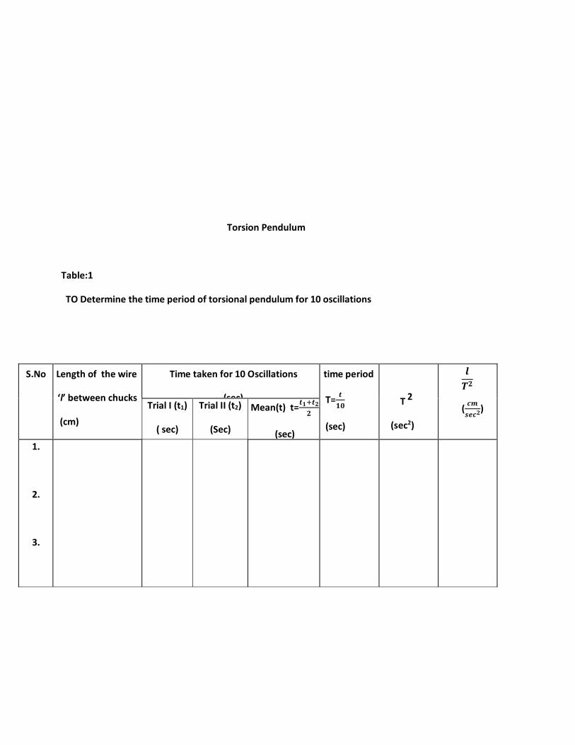
Torsion Pendulum
Table:1
TO Determine the time period of torsional pendulum for 10 oscillations
S.No Length of the wire
‘l’ between chucks
(cm)
Time taken for 10 Oscillations
(sec)
time period
T=𝒕
𝟏𝟎
(sec)
T 2
(sec2)
𝒍
𝑻𝟐
(𝒄𝒎
𝒔𝒆𝒄𝟐) Trial I (t1)
( sec)
Trial II (t2)
(Sec)
Mean(t) t=𝒕𝟏+𝒕𝟐
𝟐
(sec)
1.
2.
3.
4.
5.
6.

TORSIONAL PENDULUM
AIM:
To determine the rigidity modulus (η) of the material of the given wire using torsional
pendulum.
APPARATUS:
Torsion pendulum, wire, Stop clock, meter scale, and vernier caliper, Screw Gauge,
Electrical balance
THEORY:
When the suspension wire is twisted by the circular disc fixed at the bottom of the wire, the wire
undergoes shearing strain. This is called torsion. Because of this torsion, the disc executes oscillations
called torsional oscillations. The angular acceleration of the disc is proportional to its angular
displacement and is always directed towards its mean position. Hence, the motion of the disc is simple
harmonic.
A torsional pendulum is a flat disk, suspended horizontally by a wire attached at the top of the
fixed support.When the disk is tuned through a small angle, the wire is twisted .On being released
the disk performs torsional oscillations about the axis of the support .The period of oscillations is given by
T=2π√I/c ------------(1)
Where I is the moment of inertia of disc about the axis of rotation &’c’is the couple per unit twist of
the wire.
But
c = (πηa4 ) ----------------(2)
2l

Where a is the radius of the wire,
l is its length and
η is the rigidity modulus
from eq’s 1&2 we have,
η=8πI ( l/T2) -----------------(3)
a4
In case of a circular disc(or cylinder) whose geometric axis coincides with the axis of
rotation,the moment of inertia I is given by
I = MR2 ------------------ (4)
2
Where M is the mass of the disc
R is the radius
On substituting eq (4) in (3)
η = 4𝜋𝑀𝑅2
𝑎4 (𝑙
𝑇2) dynes/cm2
M is Mass of the disc
R is Radius of the disc
a is Radius of the wire
l is Length of the wire between the two chuck nuts
T is Time period
Table: - 2
Radius of the wire (a)

Screw gauge error = correction (n) = L.C. =
S.No. PSR
(x) (mm)
HSR
Corrected
HSR(n1)=HSR±n
y= (n1 x LC ) Diameter (d) = x + y
(mm) Radius (a)=
𝒅
𝟐
(mm)
1.
2.
3.
4.
GRAPH:-
A graph is drawing between “l “on X-axis and T2 on Y-axis.
T2
(se
l (cm)
PROCEDURE

Torsional pendulum consists of a uniform circular metal (brass or iron) disc of diameter about 10cm and
thickness of 1 cm. Suspended by a metal wire (whose η is to be determined) at the center of the
disc.The other end of the wire is griped into another chuck, which is fixed to a wall bracket. The
length (l) of wire between the two chucks can be adjusted and measured using meter scale .An ink mark
is made on the curved edge of the disc. A vertical pointer is kept in front of the disc such that the
pointer screens the mark when straight. The disc is set into oscillations in the horizontal plane, by
turning through a small angle .Now stopwatch is started and time (t) for 20 oscillations is noted.
This procedure is repeated for two times and the average value taken. The time period T (=t/20) is
calculated. The experiment is performed for five different lengths of the wire. And observations are
tabulated in table. The diameter and hence the radius (a) of the wire is determined accurately at least at
five different places of the wire using screw gauge , since the radius of the wire is small in magnitude and
appears with forth power in the formula of rigidity modulus.
The mass (M) and the radius (R) of the circular disc are determined by using rough balance and
vernier respectively.
OBSERVATION S:
Mass of the disc (M) = ------------ gm
Radius of the disc (R) = ------------- cm
Radius of the wire (a) = ------------- cm
Average of l/T2 (from table) = -----------cm/sec2
Value of l/T2 (from graph) = ------------- cm/sec2
(1N/m2 = 10 dynes /cm2 )
( 1 N = 105 dynes)
PRECAUTIONS:
1. The wire should be free from kinks. 2. The disc should not wobble. 3. The reading should be made correctly.

RESULT:
The Rigidity modulus (η) of given wire is (from table) dyne/cm2
The Rigidity modulus (η) of given wire is (from graph) dyne/cm2
Conclusion : The given wire is made up of---------------- material.
DIAGRAM: - Interference in thin air film
Eye piece
Plano convex lens
Plain glass
plate

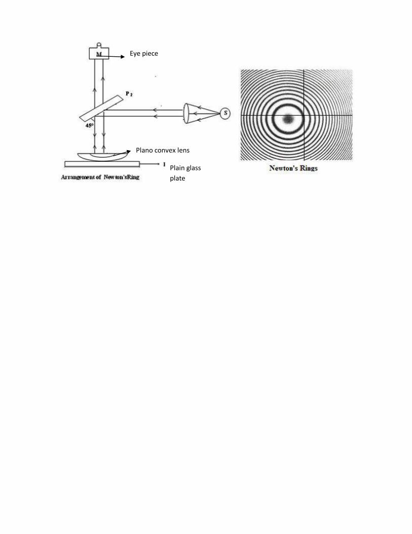
NEWTON’S RINGS EXPERIMENT
AIM: - To find the radius of curvature of the surface of the lens, by forming Newton’s rings.
APPARATUS: - Traveling micro scope, Sodium vapour lamp, Plano convex lens, 450 angle glass plate set
up, Reading lens, Reading lamp.
THEORY: -
Newton’s rings are formed because of the interference between the waves reflected from top and bottom surfaces of the air film formed between the plain glass plate and plano-convex lens. When light incident on combination of glass plate and plano-convex lens system one part of the ray will be reflected back from glass-air interface without any phase difference and the same ray is reflected from glass plate with phase difference of π. Because of interference between these two rays with phase and without phase there will be formation of circular rings.
The radius of curvature of the curved face of the lens is:
Where Dm=Diameter of the mth ring.
Dn=Diameter of the n th ring.
λ = Wave length of Sodium vapor lamp.(5893A0)
m= mth fringe
n = nth fringe
PROCEDURE: -
The apparatus consists of a light source. The light from it is rendered parallel by means of a convex lens. The parallel rays are incident on a plane glass plate through the magnifying glass inclined at 45º to the path of incident rays. Alternate bright & dark rings are observed through a traveling microscope.
The point of intersection of cross wires in the microscope is brought to the center of ring system,
R = 𝑫𝒎
𝟐 −𝑫𝒏𝟐
𝟒𝛌 ( 𝐦−𝐧) cm or A
0------------ (1)

if necessary, turning the cross wires such that one of them is perpendicular to the line of travel of
the microscope. The wire may be set tangential to any one ring; & starting from the center of the
ring system, the microscope is moved on to one side, say left, across the field of view counting
the number of rings. After passing beyond 25th ring, the direction of motion of the microscope is
reversed and the cross wire is set at the 20th dark ring, tangential to it. The reading on the
microscope scale is noted. Similarly, the readings with the cross-wires set on 18th, 16th, 14th, ---- 2nd dark
ring is noted. The microscope is moved in the right direction from the center and corresponding to the 2nd,
4th, 6th-------20th dark ring on the right side are noted. Readings are to be noted with the microscope moving in one & the same direction to avoid errors due to
backlash. The observations are recorded in table 1.The Plano convex lens is taken out from the traveling microscope and the radius of curvatureis determined by a spherometer.
OBSERVATIONS:
1. Wave length of Sodium vapour lamp (λ)
2. Least count of travelling microscope = 1 MSD/VS =
TABLE: To determine the square of the diameter of the different fringes

No. of
Ring
Microscope Reading Left side
(L)
Microscope Reading Right side
(R)
Diameter(D)
T.R L ~ T.R
(cm )
D2
(Cm2) MSR
(a)
(Cm)
VC
(b)
T.R L=a+(b x LC)
(Cm)
MSR
(a)
(Cm)
VC
(b)
T.R R=a+(b xLC)
(Cm)
20
18
16
14
12
10
8
6
4
2

GRAPH:
A graph is drawn with the number of rings as abscissa (X-axis) and the square of diameter of the ring as ordinate (Y-axis). The nature of the graph will be a straight line as shown in the fig.
From graph the values of Dı² and D2 ² corresponding to two number n1 and n2 are noted. Using these values in equation (1) the wavelength of the source λ is calculated.
To determine the radius of curvature, R, of the lens; the wavelength, λ of the source used is to be taken from standard tables.
Y
Dm²
D² (cm2)
D n ²
n m X
no. of fringes
PRECAUTIONS:
1. Wipe the lens and glass plates with cloth before starting the experiment.
2. The center of the ring must be dark.
3. Use reading lens with light while observing the readings. 4. Before starting the experiment make sure that the movement of microscope in both sides (left and
right side) of the rings.
RESULT:
The radius of curvature of Plano - convex lens is = cm/A0

Ray Diagram :
Table : To determine total number of lines on plain transmission grating .
Distance
between
grating
and
screen
(D)
(cm)
Order
Left side
d1
(cm)
Right side
d2
(cm)
Mean
d= (d1+d2)/2
(cm)
𝒔𝒊𝒏𝜽
=𝒅
√𝒅𝟐 + 𝑫𝟐
(cm)
N = 𝐝𝐬𝐢𝐧Ө
𝒏𝝀
1
2
3
4
Avg =
Experiment-11
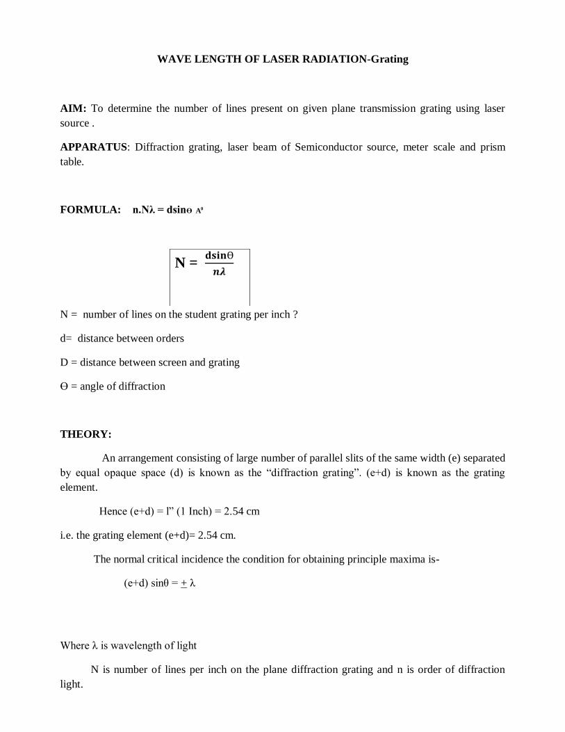
WAVE LENGTH OF LASER RADIATION-Grating
AIM: To determine the number of lines present on given plane transmission grating using laser
source .
APPARATUS: Diffraction grating, laser beam of Semiconductor source, meter scale and prism
table.
FORMULA: n.Nλ = dsinӨ A0
N = number of lines on the student grating per inch ?
d= distance between orders
D = distance between screen and grating
Ө = angle of diffraction
THEORY:
An arrangement consisting of large number of parallel slits of the same width (e) separated
by equal opaque space (d) is known as the “diffraction grating”. (e+d) is known as the grating
element.
Hence (e+d) = l” (1 Inch) = 2.54 cm
i.e. the grating element (e+d)= 2.54 cm.
The normal critical incidence the condition for obtaining principle maxima is-
(e+d) sinθ = + λ
Where λ is wavelength of light
N is number of lines per inch on the plane diffraction grating and n is order of diffraction
light.
N = 𝐝𝐬𝐢𝐧Ө
𝒏𝝀

PROCEDURE:
Keep the grating in front of the laser beam such that light is incident normally on it. When
light of laser falls on the grating the central maxima along with four other orders with decrease in
intensity are seen on the screen. The light next to central maxima is first order and light next to first
order is second order maxima.
Now measure the distance between the grating and the screen and tabulate it as
“d1” on left side and the distance between central maxima to first order on the right side is “d2” and
take the average of the “d1” “d2” .The same procedure is followed for the second order.
Substitute the values for Sin θ and determine the values of wavelength of laser
radiation.
PRECAUTIONS:
1) Do not look at the laser beam directly.
2) The prism table should be perpendicular to the laser.
3) Laser beam and the grating should be horizontal.
RESULT:
The total number of lines present on given plane transmission grating = ----------

Prism table
Direct reading
Telescope(T1 & T2)

EXPERIMENT: DISPERSION OF LIGHT (Spectrometer – Prism)
AIM: - To determine the dispersive power of the material of the given prism by the spectrometer.
APPARATUS: - Spectrometer, Source (Mercury Vapour Lamp), Prism, Magnifying
lens with light , Spirit level
THEORY: -The essential parts of the spectrometer are: (a) The telescope, (b) The
collimator & (c) Prism table.
(a) The Telescope: -
The telescope is an important part in Telescope. At one end of a brass tube is an
objective, at the other end a (Rams den’s) eyepiece and in between, a cross wire
screen. The eyepiece may be focused on the cross-wires and the length of the
telescope may be adjusted by means of a rack and pinion screw. The telescope is
attached to a circular disc, which rotates symmetrically about a vertical axis and
carries a main scale, divided in half-degrees along its edges. The telescope may be
fixed in any desired position by means of a screw & fine adjustments made by a
tangential screw.
(b) The Collimator: -
The collimator consists of a convex lens fitted at one end of a brass tube and an
adjustable slit at the other end. The distance between the two may be adjusted by
means of a rack and pinion screw. The collimator is rigidly attached to the base of
the instrument.
(c) The Prism Table: -
The prism table consists of a two circular brass discs with three leveling screws

between them. A short vertical brass rod is attached to the center of the lower disc
& this is fitted into a tube attached to another circular disc moving above the main
scale. The prism table may be fixed on the tube by means of a screw. The second
circular disc moving over the main scale carries two verniers at diametrically
opposite points. The vernier disc also revolves about the vertical axis passing
through the center of the main scale and may be fixed in any position with the
help of a screw. A tangential screw is provided for fine movements of the vernier
scale.
Most Spectrometers have 29 main scale divisions (half-degrees) divided on the
vernier into thirty equal parts. Hence, the least count of the vernier is one-
sixteenth of a degree or one minute.
OBSERVATIONS: -
Least count of the vernier of the spectrometer LC =
Angle of prism A =
Direct reading Vernier (LHS) V1= MSR + (VCXLC) =
Vernier (RHS) V2= MSR + (VCXLC) =
Table : Angle of prism (A)

S No Telescope reading left side Telescope reading right side 2A=
T.RL ͠T.RR
A= 𝐓.𝐑𝐋 ͠𝐓.𝐑𝐑
𝟐
M.S.R
(a) Degree
V.C
(b)
T.RL= a+(b x LC) M.S.R
(a) Degree
V.C
(b)
T.RR= a+(b x LC)
Table : Direct Reading
Telescope reading
MSR (a) V.C (b) T.R = a+ ( b x LC )
TABLE :- Angle of minimum deviation ( δm / Dm)

Preliminary Adjustments: -
The following adjustments are to be made before the commencement of an
experiment with spectrometer.
(i) Eyepiece Adjustment: -
The telescope is turned towards a bright object, say a white wall about 2 to 3
colors Reading of the deviated ray Angle of deviated
ray
Mean
(D)
𝑋 + 𝑌
2
µ = sin(
𝐴+𝐷
2)
sin(𝐴
2)
LHS (VL) RHS(VR)
V1~ VL
(X)
V2~ VR
(Y)
MSR
(a)
VC
(b)
T.R =a+(b x LC)
(VL)
MSR
(a)
VC
(b)
T.R =a+(b x LC)
(VR)
Blue
Red
Green
Violet
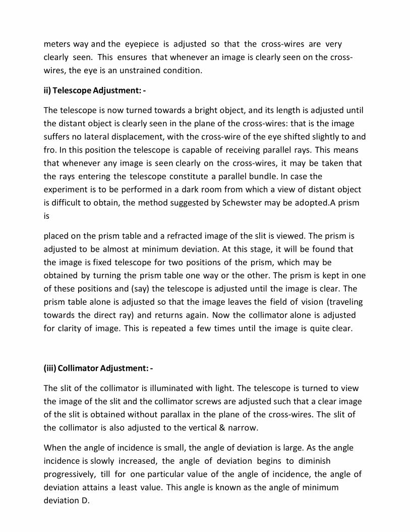
meters way and the eyepiece is adjusted so that the cross-wires are very
clearly seen. This ensures that whenever an image is clearly seen on the cross-
wires, the eye is an unstrained condition.
ii) Telescope Adjustment: -
The telescope is now turned towards a bright object, and its length is adjusted until
the distant object is clearly seen in the plane of the cross-wires: that is the image
suffers no lateral displacement, with the cross-wire of the eye shifted slightly to and
fro. In this position the telescope is capable of receiving parallel rays. This means
that whenever any image is seen clearly on the cross-wires, it may be taken that
the rays entering the telescope constitute a parallel bundle. In case the
experiment is to be performed in a dark room from which a view of distant object
is difficult to obtain, the method suggested by Schewster may be adopted.A prism
is
placed on the prism table and a refracted image of the slit is viewed. The prism is
adjusted to be almost at minimum deviation. At this stage, it will be found that
the image is fixed telescope for two positions of the prism, which may be
obtained by turning the prism table one way or the other. The prism is kept in one
of these positions and (say) the telescope is adjusted until the image is clear. The
prism table alone is adjusted so that the image leaves the field of vision (traveling
towards the direct ray) and returns again. Now the collimator alone is adjusted
for clarity of image. This is repeated a few times until the image is quite clear.
(iii) Collimator Adjustment: -
The slit of the collimator is illuminated with light. The telescope is turned to view
the image of the slit and the collimator screws are adjusted such that a clear image
of the slit is obtained without parallax in the plane of the cross-wires. The slit of
the collimator is also adjusted to the vertical & narrow.
When the angle of incidence is small, the angle of deviation is large. As the angle
incidence is slowly increased, the angle of deviation begins to diminish
progressively, till for one particular value of the angle of incidence, the angle of
deviation attains a least value. This angle is known as the angle of minimum
deviation D.

FORMULA :-
The refractive index of the material of the prism is given by
2sin
2sin
A
DmA
Where A is the angle of the equilateral prism and
Dm is the angle of minimum deviation.
The dispersive power (ω) of the material of the prism is given by
1
RB
Where µB= the refractive index of the blue rays
µR = the refractive index of the red ray and
2
RB ; the mean of µB and µR
PROCEDURE: -
1. The prism is placed on the prism table with the ground surface of the prism
on to the left or right side of the collimator. The vernier table is then fixed

with the help of vernier screw. 2. The ray of light passing through the collimator strikes the polished surface BC
of the prism and undergoes deviation.And emerges out of the prism from the face AC.
3. The deviated ray (continuous spectrum) is seen through the telescope in
position T1. Looking at the spectrum the prism table is now slowly moved on
to one side, so that the spectrum moves towards undeviated path of the
beam.
4 . The deviated ray (spectrum) also moves on to the same side for some time
and then the ray starts turning back even through the prism table is moved in
the same direction. The point at which the ray starts turning back is called
MINIMUM DEVIATION POSITION.
5 . In the spectrum, it is sufficient if one colour is adjusted for minimum
deviation position. In this limiting position of the spectrum, deviation of
the beam is minimum.
6. The telescope is now fixed on the blue colour and the tangent screw is
slowly operated until the point of intersection of the cross wire is exactly on
the image. The reading for the blue colour is noted in vernier 1 and vernier 2
and tabulated. The reading is called the minimum deviation reading for the
blue colour.
7. The telescope is now moved on the red colour and the readings are taken as
explained for blue colour.
8. Next, the telescope is released and the prism is removed from the prism
table. The telescope is now focused on to the direct ray (undeviated path)
and the reading in vernier 1 and vernier 2 are noted.
9. The difference of readings between the deviated reading for blue colour and
the direct reading gives the angle of the minimum deviation for the blue colour.
10. Similarly, the difference of readings between the deviated reading for the
red colour and the direct reading gives the angle of minimum deviation for
the red colour.
11. The refractive indices for the blue and red rays are calculated using
equation and the dispersive power of the material of the prism is
calculated.(the angle of the equilateral prism, A = 60°).

PRECAUTIONS:
1. Don’t touch polished surface of the prism with hands to avoid finger prints. 2. Use reading lens with light while taking the readings in vernier scale. 3. The mercury light should be placed in side a wooden box.
RESULT:
Dispersive power of the material of the prism (ω) = ------------
Dispersive power of crown material = -------
Hence the given material of prism is ------------------
CIRCUIT DIAGRAM

GRAPH:
OBSERVATIONS:
Self inductance of the coil, L =
Capacity of the condenser, C =
Resistance of the resistor, R =
Input voltage of the A.C, Vi= volt
S.No. Frequency f(KHz) Current, I(mA)

LCR - Series Resonance
AIM:
To study the frequency response characteristics of L.C.R. Series resonance circuit and to determine
the resonance frequency and quality factor.
APPARATUS:
A signal generator, vacuum tube voltmeter, a milli ammeter, condenser, an inductance coil, a
resistance box and connecting wires.
FORMULA:
Theoretical Formula:
1. Resonance frequency of the series resonant circuit is,
fo = LC2
1
2. Quality factor of the circuit is,
Q = C
L
R
1
Where R = resistance of the resistor (ohm)
L = inductance of the coil (henry)
C = capacitance of the condenser (farad)
Experimental Formula:
1. Resonance frequency of the circuit, fo = Hz
(From the graph)
2. Bandwidth of the resonant circuit, ∆f = (f2- f1)
(From the graph)
Where f1 = lower half power frequency

f2 = upper half power frequency
3. Quality factor of the circuit, Q = f
fo
THEORY:
A coil of self inductance L, resistance R and condenser of capacitance C are connected in series
with a source of A.C.Supply as shown in the circuit. This circuit is known as L.C.R.circuit. Where an
alternating voltage of a pure sine waveform which is represented by,
E = Eo sin t
Is applied to the circuit, then an A.C. will flow through the circuit. The current flowing through the circuit at
any instant is given by,
I = Io sin t
Where E = instantaneous value of the applied voltage
Eo = maximum or peak value of the alternating voltage.
I = instantaneous value of the current
Io = maximum or peak value of the current
= angular frequency of the A.C supply
= 2 f
f = frequency of the alternating voltage
t = phase angle
= 2 f t
Due to the applied E.M.F i) an E.M.F ( L dt
di) is induced in the inductance which oppose the applied
E.M.F ii0 there is a potential drop (Ri) across the resistance and iii) a potential difference (Q?C) is developed
across the plates of the condenser, then, according to Ohm’s law,
Eo Sin RIC
Q
dt
dILt

tSinERIC
Q
dt
dIL o
Where Q = charge on the plates of the condenser at an instant
I = instantaneous value of the current in the circuit
The peak value of the current is given by
2
2 1
CLR
EI o
= 22 )( CL
o
XXR
E
Where, XL = fLL 2 inductive reactance of the circuit
XC =fcc 2
11 = capacitive reactance of the circuit
The total resistance offered to flow of current in the A.C.circuit is called the impedance (z) of the circuit or
effective resistance of the circuit.
The impedance of the circuit z=
2
2 1
CLR
Io = Z
Eo
The phase difference between the current in the circuit and the E.M.F applied to the circuit is given by,
R
CL
Tan
1
From above equation, it is obvious that whether the current in the A.C.circuit leads the E.M.F or lags behind
the E.M.F. depends on the magnitude of the inductive reactance, L as well as on the capacitive reactance
C.
Special case:When, C
L
1
, then Tanθ = 0, Z=R and I=R
Eo
In this case, the current and the applied E.M.F are in phase with each other. This condition is known as
resonance. So, the current in the circuit depends only on the value of R. If the value of R is small, the

impedance of the circuit is minium. Consequently, maximum A.C will flow through the circuit and the circuit
is said to be in tune or resonance with the applied voltage. The frequency at which L =C
1
Is called the resonance frequency, fo and the circuit is known as the series resonance circuit.
L =C
1
orLC
12
LC
o
1 , = o at resonance
LC
fo
12
LCfo
2
1
PROCEDURE:
A coil of self inductance L , a condenser of capacity C , a resistance R(10 ) and a milliammeter a
are to be connected in series with the signal generator as shown in the circuit. Switch on the signal
generator. Adjust the frequency nob of the signal generator so that the frequency, f of the A.C.signal is 2
KHz. Adjust the amplitude of the input signal to a convenient value by means of V.T.V.M. i.e., the input
voltage Vi. Then, note the current I, in the circuit shown by the milliammeter A.
Increase the frequency, f of the input signal in convenient steps (say 1 KHz), keeping input voltage,
Vi constant throughout the experiment. Then the current increases slowly at the beginning, afterwards
increases sharply and then reaches a peak value called the sharpness of the resonance. This will happen
when the frequency of the applied voltage is equal to the natural frequency of the circuit i.e., resonance
occurs. This frequency at which the current reaches a peak value is called the resonance frequency, fo. At
the resonance frequency, the current is maximum and the impedance is minimum. Again increase the
frequency of the input signal beyond the resonance frequency, and then the current through the circuit
gradually decreases. Note the observations in table.
Repeat the experiment b introducing different values of R in the circuit, for the same values of L
and C, keeping the input voltage Vi constant throughout the experiment. The theoretical values of the
resonance frequency, fo and the quality factor, Q can be calculated using the formulae.
GRAPH:
Draw a graph with the frequency, f on the x-axis and the current I on the y-axis. A sharp resonance
curve will be obtained. From the graph, note the maximum current, Io and thecorresponding frequency at
which the current is maximum. This frequency is called as the resonance frequency f0.
To determine the bandwidth (∆f ) and quality factor Q:
From the graph, find the value of Io/ 2 . Mark the value on the y-axis. From the value draw a line
parallel to x-axis. This line cuts the curve at two points A,B< called half power points. From the points A and

B, draw lines parallel to y-axis, which meets the x-axis at two points corresponding to two frequencies f1
and f2 called the half power frequencies, on either side of the resonance frequency fo.
Bandwidth of the circuit, ∆f = (f2- f1) KHz
Quality factor of the circuit, Q = f
fo
Also draw a graph with frequency f, along the x-axis and the impedence Z along the y-axis.The theoretical
and experimental values of the resonance frequency fo and the quality factor Q are to be compared.
CALCULATIONS:
1. Theoretical values:
i) L = ----------henry C = --------farad R = -----------
Resonance frequency, fo = LC2
1 = --------------Hz
iii) Quality factors, Q = C
L
R
1= ---------
Experimental values (From graphs)
i)Resonance frequency,f0 = ------KHz = ------Hz
ii) Band width, f = (f2 – f1) = ------KHz = -------Hz
iii)Quality actor Q = f
f
0 = -----
PRECAUTIONS:
1. A fixed amplitude of voltage should be applied to the circuit for the selected values of L,C and R at different frequencies.
2. The input voltage applied to the circuit should be checked at all the frequencies.
RESULT:
The theoretical and experimental values of resonance frequency, fo and the quality factor Q, are
calculated and compares. They are found to be equal.

S.No. Type of connection Parameter Theoretical Experimental
L1C1R1 L1C1R1
1 Series Resonance
Resonance frequency
foHz
2 Quality factor Q

Lab 2: coupled oscillators
1 Introduction
In this experiment you are going to observe the normal modes of oscillation of several different me-
chanical systems, first on the air tracks and then using some coupled pendula. The normal modes of
motion of a system of coupled oscillators are ‘stable’ with respect to time. That is, if you start the
masses of a system oscillating in one of the normal modes and observe it for some time, the motion will
have constant characteristics as its amplitude decays because of the ever present friction forces. Also,
the frequency of oscillation of all the masses in the system is the same, and each of the masses
executes simple harmonic motion at this frequency. The frequency is called the natural frequency of the
normal mode or an eigenfrequency of the system. There are certain relationships between the
eigenfrequencies and the frequencies of the uncoupled oscillators that will be discussed later. If a system is excited into oscillations that are a mixture of normal modes, then the motion will
change character over a period of time. Perhaps one of the masses will decrease amplitude and pass
its energy to another mass, which will later pass the energy back. Such motion is clearly different from
simple harmonic motion and therefore does not constitute a normal mode, even though the oscillations
are all at the same frequency. The exchange of energy generally occurs at a frequency that is quite
different from the oscillation frequency. (Read this paragraph a second time.)
2 Theory
Begin your study with two equal mass gliders on the air track as shown in Fig. 1. If the masses are
not equal, certain complications arise that can obscure the simplicity of the motion, so you should
remove all extra weights, clips, etc. and be sure that you have two sails of equal mass that you can
mount on these gliders for damping the motion by air friction. The two gliders are coupled together
with a spring as shown in the diagram. This coupling is somewhat tighter than the coupling you will
later use with the two pendula, but it is not perfectly rigid; with a rigid bar the system would have
only one mode of oscillation because the gliders would not be able to move relative to one another.
M M
to
X
motor
X1 X 2 3
Figure 1: The two masses and
three spring constant are
equal. At equilibrium, the three
lengths xi are also equal. The
motor can only drive one end
of one spring, but at reso-
nance the energy is distributed
among the masses.
If you displace the gliders symmetrically from their initial equilibrium positions and release them,
their oscillations will die down in time, but the relative displacements of the two gliders will maintain a
constant relationship. For example, if you push them toward one another by the same amount and
release them, the displacement of one will always be equal in magnitude but opposite in direction

the displacement of the other. If you displace them both to one side by an equal amount
and release them, they will oscillate together in a way that preserves their equilibrium
separation. You should be able to observe both of these normal modes of oscillation with
the pair of coupled masses before you go any further. You should observe that the two normal modes described above have different
frequencies. Mea-sure these frequencies. You should rotate the sails on the gliders so that they are parallel to the air track to minimize damping in order to do this part of the experiment. There will then be many oscil-lations for you to count before all the energy of the system is lost. Now hold one of the masses fixed and measure the oscillation frequency of the other mass. Also, fix the second mass and measure the oscillation frequency of the first one. What is
the relationship among the four frequencies you have measured? q In the case of one mass vibrating with the other held fixed the frequency is simply ! = 2k=M
since the restoring force on the displaced mass is 2kx (because there are two springs each con- tributing kx). For the oscillations with the distance between the gliders constant, the frequency is q ! = 2k=2M since there might just as well be a massless rigid bar between the gliders making it a mass of 2M oscillating under the same conditions as the single mass above. For the case of the q masses oscillating in opposite directions, the frequency is ! = 3k=M since the restoring force from the middle spring is 2kx (its stretch is twice the displacement of either mass) plus the normal restor-ing force from the outside spring. The frequencies you measure
should therefore be in the ratio of 1 : p
2 : p
3. Also notice that the sum of the squares of
the individual oscillation frequencies (first one mass fixed and then the other) is equal to the sum of the squares of the frequencies of the normal modes. This is not an accident!
It is constructive to consider the motion of the center of mass (CM) of the system of
gliders in each of the normal modes. In this case it is easy: in the high frequency mode
(called the optical mode) the CM remains fixed at the middle of the center spring. You can
hold the spring at this point without disturbing the oscillation. This point is called a node of
the motion. In the low frequency normal mode (called acoustical mode) the CM oscillates
at the acoustical frequency. In the optical mode there is motion with respect to the CM, but
the CM is stationary. In the acoustical mode there is no motion with respect to the CM, but
the CM moves. These are general properties of these two types of modes. Consider the motion of the gliders with respect to the CM. How does the motion look from a
coordinate system moving with the CM in each of the normal modes of oscillation? Describe it.
3 Procedure
The normal modes of motion represent the way a system of coupled masses oscillates naturally. In
order to see what happens to a system of coupled oscillators driven at some frequency, consider the
analogy to the case of a single mass where the motion is oscillatory at the driving frequency with an
amplitude that is a maximum when the driving frequency is equal to the natural frequency. Since the
coupled oscillators have two natural frequencies you might expect there to be two resonant maxima in
the amplitude of the driven motion. In order to test this, you should mount the sails on the gliders for
damping and proceed to drive them at various frequencies using the variable speed motor. You should
record the amplitude of oscillation of each mass as a function of the driving frequency and plot the
result. You should observe two resonant maxima for each mass as shown in Fig. 2, and the maxima
2
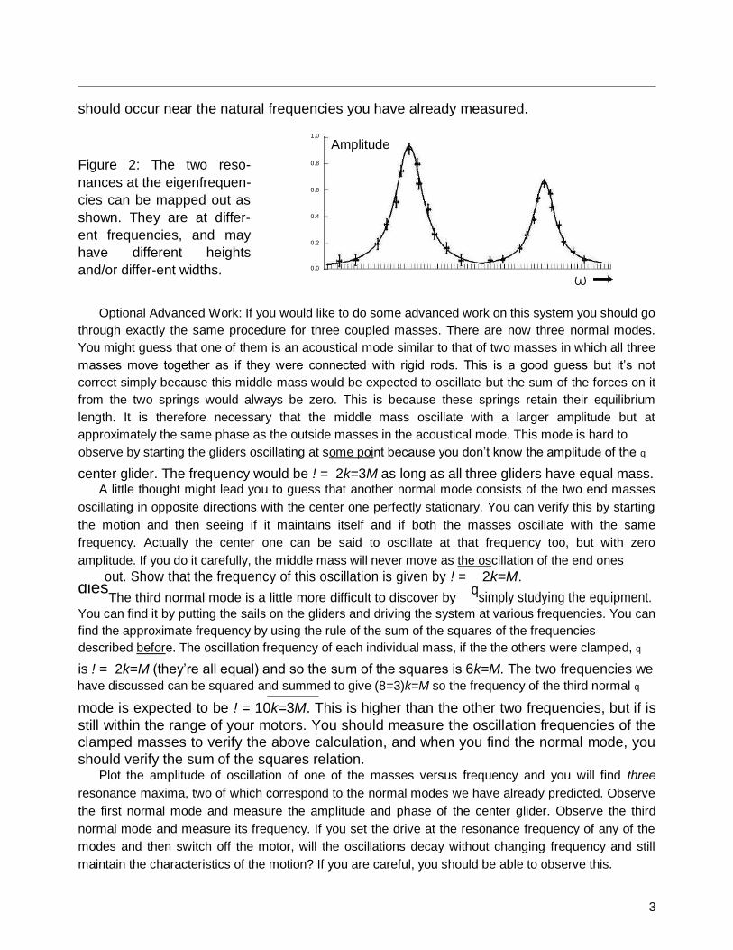
should occur near the natural frequencies you have already measured. Figure 2: The two reso-
nances at the eigenfrequen-
cies can be mapped out as
shown. They are at differ-
ent frequencies, and may
have different heights
and/or differ-ent widths.
1.0
Amplitude 0.8
0.6
0.4
0.2
0.0
ω
Optional Advanced Work: If you would like to do some advanced work on this system you should go
through exactly the same procedure for three coupled masses. There are now three normal modes.
You might guess that one of them is an acoustical mode similar to that of two masses in which all three
masses move together as if they were connected with rigid rods. This is a good guess but it’s not
correct simply because this middle mass would be expected to oscillate but the sum of the forces on it
from the two springs would always be zero. This is because these springs retain their equilibrium
length. It is therefore necessary that the middle mass oscillate with a larger amplitude but at
approximately the same phase as the outside masses in the acoustical mode. This mode is hard to observe by starting the gliders oscillating at some point because you don’t know the amplitude of the q center glider. The frequency would be ! = 2k=3M as long as all three gliders have equal mass.
A little thought might lead you to guess that another normal mode consists of the two end masses
oscillating in opposite directions with the center one perfectly stationary. You can verify this by starting
the motion and then seeing if it maintains itself and if both the masses oscillate with the same
frequency. Actually the center one can be said to oscillate at that frequency too, but with zero
amplitude. If you do it carefully, the middle mass will never move as the oscillation of the end ones
out. Show that the frequency of this oscillation is given by ! = 2k=M. dies
The third normal mode is a little more difficult to discover by q
simply studying the equipment. You can find it by putting the sails on the gliders and driving the system at various frequencies. You can
find the approximate frequency by using the rule of the sum of the squares of the frequencies described before. The oscillation frequency of each individual mass, if the the others were clamped, q is ! = 2k=M (they’re all equal) and so the sum of the squares is 6k=M. The two frequencies we have discussed can be squared and summed to give (8=3)k=M so the frequency of the third normal q mode is expected to be ! = 10k=3M. This is higher than the other two frequencies, but if is
still within the range of your motors. You should measure the oscillation frequencies of the
clamped masses to verify the above calculation, and when you find the normal mode, you
should verify the sum of the squares relation. Plot the amplitude of oscillation of one of the masses versus frequency and you will find three
resonance maxima, two of which correspond to the normal modes we have already predicted. Observe
the first normal mode and measure the amplitude and phase of the center glider. Observe the third
normal mode and measure its frequency. If you set the drive at the resonance frequency of any of the
modes and then switch off the motor, will the oscillations decay without changing frequency and still
maintain the characteristics of the motion? If you are careful, you should be able to observe this. 3

Consider the motion of the CM of the three coupled oscillators. Describe the motion of
the CM for each of the three normal modes of oscillation. Describe the motion of each of
the gliders with respect to the CM for each of the three normal modes. Could you do this
for motion of the system which is a mixture of normal modes?
4 Hints and Kinks Department
You must remember to wait some time for oscillations at the undesirable frequencies to die out
after you change the driving frequency of the variable speed motor. Otherwise you will have the
kind of problems of mixed modes described at the end of Experiment 1, namely, the motion will be
a super-position of two or more frequencies. With coupled oscillators the system is much more
complicated and too difficult to analyze in that simple way, so it’s important to be patient. The damping time of an air track glider with sail is also considerably longer than the
spring in Experiment 1. You may want to measure it by clamping one glider and just
watching the other one’s oscillations damp out (of course, with no drive). Suffice it to say
that the motion at any frequency which is not a pure eigenfrequency will decay into a
superposition of the normal modes of the system resulting in a rather complicated motion. It is very important to match the masses of the system as closely as possible. If you don’t,
the normal modes will not be symmetrical in the coordinate displacements. Of course normal
modes exist for any system, whether or not the masses are equal. Usually the displacements
are inversely proportional to the masses so that the CM of the system behaves in the same
way as the center-of-mass of a system with equal masses. Remember that the sails do not
have zero mass, so that the measurements you make of the resonant frequencies with other
masses clamped should have the sails mounted but turned parallel to the track. Be sure you do not drive the system into oscillations that are so large that the springs
pop off. Be careful not to overheat the motors.
5 Coupled Oscillators With Variable Coupling
Connect the strings of two pendula with a massless (almost) rigid rod such as a soda straw.
You can do it by cutting short slits in the ends of the straw and slipping the string of each
pendulum into the slits at the end of the straw. The distance between the pendulum strings
should be just a few mm less than the length of the straw. You should slide the coupling rod up
the string until 9/10 or more of the string is below the coupling. Find and describe the normal
modes of oscillation in the plane of the strings of this system of coupled oscillators (hint: there
is an acoustical and an optical mode). What are the frequencies? Show that the measured
values of the frequencies are consistent with the expected values. Do they also satisfy the sum
of the squares rule? (How would you ‘clamp’ one of the masses in this case?) You should observe and measure the frequencies of the normal modes for several different heights
of this coupling bar. Make a plot of the frequencies of the normal modes versus height of the coupling
bar. Is the result what you expect? Why or why not? Prove that the frequency of one of the normal
modes is independent of the height of the bar, and that the other normal frequency depends on the
4
PHY 300 Lab 2 Fall 2009
square root of the distance from the bar to the pendulum bob. Which is the optical mode
and which is the acoustical? Put the bar near the top of the strings, displace one of the pendulum bobs, and release it. What
happens? Describe the motion in detail. Go back and read the second paragraph of this write-up for a
third time. How long does the phenomenon you observe take? This time depends on the degree of
coupling and therefore on the height of the bar. Measure the time it takes versus height of the bar and
make a graph. Does the curve look familiar? Is it related to anything we have done before? Is it related
to the eigenfrequencies? How? Plot the time for energy transfer versus eigenfrequency to find out.
Speculate on the formula for the time versus bar height graph. Can you derive it? If you put the bar too low (lower than about 1/2 of the length of the strings) you will find that
there is substantial coupling to another normal mode of oscillation, the torsional mode. Be careful
to avoid it in the measurements above, but if you choose to do advanced work on this experiment
you should study this mode as well as other normal modes of oscillation of the system. There are a
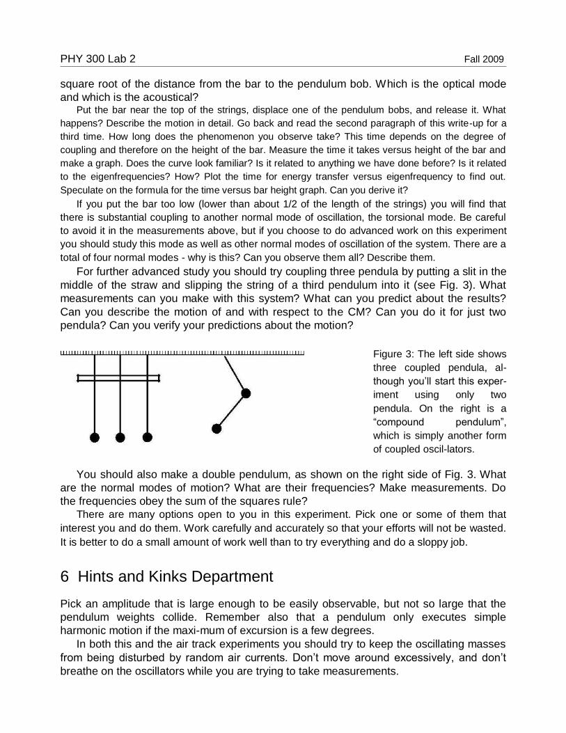
total of four normal modes - why is this? Can you observe them all? Describe them. For further advanced study you should try coupling three pendula by putting a slit in the
middle of the straw and slipping the string of a third pendulum into it (see Fig. 3). What
measurements can you make with this system? What can you predict about the results?
Can you describe the motion of and with respect to the CM? Can you do it for just two
pendula? Can you verify your predictions about the motion?
Figure 3: The left side shows
three coupled pendula, al-
though you’ll start this exper-
iment using only two
pendula. On the right is a
“compound pendulum”,
which is simply another form
of coupled oscil-lators.
You should also make a double pendulum, as shown on the right side of Fig. 3. What
are the normal modes of motion? What are their frequencies? Make measurements. Do
the frequencies obey the sum of the squares rule? There are many options open to you in this experiment. Pick one or some of them that
interest you and do them. Work carefully and accurately so that your efforts will not be wasted.
It is better to do a small amount of work well than to try everything and do a sloppy job.
6 Hints and Kinks Department
Pick an amplitude that is large enough to be easily observable, but not so large that the
pendulum weights collide. Remember also that a pendulum only executes simple
harmonic motion if the maxi-mum of excursion is a few degrees. In both this and the air track experiments you should try to keep the oscillating masses
from being disturbed by random air currents. Don’t move around excessively, and don’t
breathe on the oscillators while you are trying to take measurements.

©
FIBER OPTICS CHARACTERISTICS USER MANUAL
NOTE: DONOT INTERCHANGE FIBER OPTICS EXPERIMENT ACCESSORIES WITH ANY OTHER UNIT. STRICTLY ADHERE TO RESPECTIVE SERIAL NUMBERS PASTED ON ALL PARTS/UNITS.
Manufactured by:
MIKRON INSTRUMENT INDUSTRIES 303, Moghuls Court building, Basheerbagh Hyderabad – 1.
Ph. 040 – 6450 890 / 51 . Fax. 040 – 6662 5145 email. [email protected] / [email protected]
1

EXPERIMENT: 1 LOSSES IN OPTICAL FIBER AT 660nm AND 850nm
1.1 Aim of the Experiment:
The aim of the experiment is to study various types of losses that occur in optical fibers and measure losses in dBm of two optical fiber patch cords at two wavelengths. Viz. 660 nm and 850 nm.
Theory: Attenuation in an optical fiber is a result of following effects:
Losses at connectors and losses due to the length of the fiber cable. The optical power at a distance L, in an optical fiber is given by PL α PoL, Where Po is the input power and α is the attenuation coefficient in decibels per length. The typical attenuation coefficient value for the fiber under consideration is 0.2dBm per meter at a wavelength 660nm.
Losses in fiber occur at fiber-fiber joints or splices due to axial displacement, Angular
displacement, separation (air core), mismatch of course diameter, mismatch of numerical aperture, improper cleaving and cleaning at the ends. The loss equation for simple fiber optic link is given by:
Pin(dBm)-Pout(dBm) = Lj1+LFIB1+Lj2+LFIB2+Lj3(dB): Where Lj1(dB) is the loss at LED
connector junction, LFIB1(dB) is the loss in cable1, Lj2(dB) is the insertion loss in a line
connector, LFIB2(dB) is the loss in cable2, and Lj3(dB) is loss at the connector detector
junction.
NOTE: In this particular experiment connections to Voltmeter (M1), Signal generator are not required. Connect the circuit as mentioned below in the experiment procedure.
Experiment Procedure for IR L.E.D 850 nm ( Infra Red Light Emitting Diode ) :
We are mainly finding losses in optical fibers due to its length and bending.
Following procedure is for study of losses due to length of optical fibre using 850nm L.E.D. 1. Short M2 of I.R L.E.D ( +ve and –ve terminals ) on the Tx unit with patch cords ( for this experiment M2 is not required ) .
2. Relieve all the twists and strains in the fiber cable, ensure that it is as straight as possible, as shown in fig.1.1.
3. Connect one end of the cable 1 ( 1 meter ) to the 850nm LED FC ( Fiber Connector ) adapter of the Tx unit and other end to the PIN diode FC ( Fiber Connector ) adapter of Rx unit as shown in figure 1.1.
4. Move the S1 switch on Rx unit towards 850 nm IR LED.
5. Switch ON the AC mains of both Rx & Tx units.. 6. Rotate Po ( Power Adjustment potentiometer ) pot to extreme clockwise direction to set
maximum carrier power, note down the “Optical Power Meter Reading “ P1 in µW on Rx unit. 7. Without altering the position of Po ( Power Adjustment potentiometer ) pot, Connect cable 2 (
3meters ) between 850nm FC adapter and PIN diode FC adapter of Rx Unit. Note/Tabulate “Optical Power Meter Reading “, P2 on th Rx unit.
2

8. Without altering the position of Po ( Power Adjustment potentiometer ) pot, Connect cable 3 (
5 meters ) between 850nm FC adapter and PIN diode FC adapter of Tx Unit. Note/Tabulate “Optical Power Meter Reading “, on the Rx unit, P3 ( As per table 1.1 ).
9. Convert the all power meter readings in µW to dBm using formula. Given below. dBm=10*log (Power meter reading in mW/1mW)
In this case, dBm=10*log (Power meter reading in µW/1000) 10. Tabulate all the readings in table 1.1 11. Calculate average loss per meter at 850 nm. The loss per meter in the range of 2±0.5 dBm is acceptable ( As per standards ) .
Experiment Procedure for L.E.D 660 nm ( Light Emitting Diode ) :
Following procedure is for study of losses due to length of optical fibre using 660nm L.E.D.: 1. Short M2 of 850nm LED ( +ve and –ve terminals ) on the Tx unit with patch cords ( for this
experiment M2 is not required ) . 2. Relieve all the twists and strains in the fiber cable, ensure that it is as straight as possible, as
shown in fig.1.1. 3. Connect one end of the cable 1 ( 1 meter ) to the 660nm LED FC ( Fiber Connector ) adapter
of the Tx unit and other end to the PIN diode FC ( Fiber Connector ) adapter of Rx unit as shown in figure 1.1.
4. Move the S1 switch on Rx unit towards 660 nm L.E.D.
5. Switch ON the AC mains of both Rx & Tx units. 6. Rotate Po ( Power Adjustment potentiometer ) pot to extreme clockwise direction to set
maximum carrier power, note down the “Optical Power Meter Reading “ P1 in µW on Rx unit.
7. Without altering the position of Po ( Power Adjustment potentiometer ) pot, Connect cable 2
( 3meters ) between 660nm FC adapter and PIN diode FC adapter of Rx Unit. Note/Tabulate
“Optical Power Meter Reading “, P2 on th Rx unit.
8. Without altering the position of Po ( Power Adjustment potentiometer ) pot, Connect cable 3
( 5 meters ) between 660nm FC adapter and PIN diode FC adapter of Tx Unit. Note/Tabulate
“Optical Power Meter Reading “, on the Rx unit, P3 ( As per table 1.1 ).
9. Convert the all power meter readings in µW to dBm using formula. Given below. dBm=10*log (Power meter reading in mW/1mW)
In this case, dBm=10*log (Power meter reading in µW/1000) 10. Tabulate all the readings in table 1.1 11. Calculate average loss per meter at 660 nm. The loss per meter in the range of 0.2 dBm is
acceptable ( As per standards ) .
Experimental Procedure for losses due to OF Bending using 850nm L.E.D:
STEP 1: Short the M2 +ve and –ve terminals of both LED’s on Tx unit, and Connect one end of the cable 1mtr to the 850nm LED FC adaptar of the Tx unit and other end to the pin diode FC adaptor of Rx unit as shown in figure 1.1. Move the S2 switches on Tx unit towards 850 nm IR LED input. Then turn on the AC mains. STEP 2: Relieve all the twists and strains in the fiber cable so that it is straight as shown in fig.1.1 STEP 3: Rotate P0 pot to the extreme clockwise direction to get maximum intensity and note down the reading(P01) of power meter on Rx unit..
3
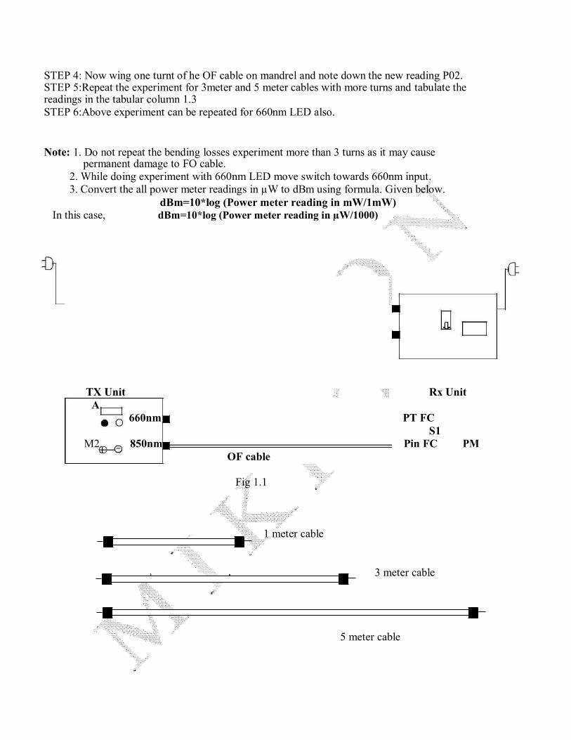
STEP 4: Now wing one turnt of he OF cable on mandrel and note down the new reading P02. STEP 5:Repeat the experiment for 3meter and 5 meter cables with more turns and tabulate the readings in the tabular column 1.3 STEP 6:Above experiment can be repeated for 660nm LED also. Note: 1. Do not repeat the bending losses experiment more than 3 turns as it may cause
permanent damage to FO cable.
2. While doing experiment with 660nm LED move switch towards 660nm input.
3. Convert the all power meter readings in µW to dBm using formula. Given below. dBm=10*log (Power meter reading in mW/1mW)
In this case, dBm=10*log (Power meter reading in µW/1000)
TX Unit Rx Unit
A
660nm PT FC
S1
M2 850nm Pin FC PM
OF cable
Fig 1.1
1 meter cable
3 meter cable
5 meter cable

4

Table 1.1
Table of readings for 850nm
SI P1 Rd1 P2 Rd2 P3 Rd3 M0=Rd1-Rd2/2 M1=Rd2-Rd3/2 M2=R1-R3/4 L/M
No. in µW(dBm)in µW(dBm) in µW (dBm) (dBm) (dBm) (dBm) (dBm)
Table of readings for 660nm
SI P1 R1 P2 R2 P3 R3 M0=R1-R2/2 M1=R2-R3/2 M2=R1-R3/4 L/M
No. in µW(dBm)in µW(dBm) in µW (dBm) (dBm) (dBm) (dBm) (dBm)
Where L= Mo + M1 + M2
3
Table 1.3 Table of readings for 850nm n=No of Turns on mandrel……… Cable P01 R01 P02 R02 R01-R02 P11 R11P12 R12 R11-R12
No of
L in µW in dBm in µW in dBm
n
in µW in dBm in µW in dBm
Turns(n)
n
1 mtr
3 mtr
5mtr
5

EXPERIMENT 2: CHARACTERISATION OF 660 NM AND 850 NM L.E.D.
Aim of the experiment 2.1: The aim of the experiment is to study the relationship between the LED dc forward current and the L.E.D. optical power output and determine the linearity of the device at 660nm as well as 850 nm. Theory: L.E.D and Laser diodes are commonly used sources in optical communication systems, whether the system transmits digital or analogue signals. In case of analogue transmission, direct intensity modulation of optical source is possible, provided the optical out put from the source can be linearly varied as a function of the modulating electrical signal amplitude. L.E.D have a linear optical out put with relation to the forward current over a certain region of operation. It may be mentioned that in many low cost, short-lenght and small bandwidth applications, L.E.D at 660nm, 850nm and 1300nm are popular. While direct intensity modulation is easy to realize, higher performance is achieved by FM modulating the base band signal prior to intensity modulation. The relationship between an L.E.D optical output Po and the L.E.D forward current Iғ is given by Pо=K *Iғ (over a limited range) where K is constant.
Experiment Procedure:
1. Connect one end of the cable1(1mtr) to the 850nm L.E.D. FC adaptor of Tx unit and the
other end to the PIN photodiode FC adaptor of Rx unit. 2. Connect on board Ammeter to 850nm IR L.E.D M2 meter (to its respective +ve and –
ve terminals) provided on the circuit panel of the Tx unit as shown in fig 2.1, Move the S2 switch on Rx unit towards 850 nm IR LED and Then turn on the AC mains.
3. Rotate Po pot to the extreme anticlockwise direction to reduce the Iғ (L.E.D. forward current) to 0Amps and power meter should be zero.
4. Slowly rotate the Po knob in clockwise direction to increase Iғ. The power meter should read 5µW approximately. 5. Now change Iғ in steps of 3mA by rotating Po in clockwise direction and note the
power meter readings. 6. Tabulate the readings as in Table 1.2. and Repeat the above complete experiment for 660nm L.E.D. also.
AC AC
Tx Unit Rx Unit
A660nm PT
P0 OF Cable
850nm Pin PM
6

M2
Fig 2.1
Table for 850nm LED
Table 1.2
SI IF in mA Power mtr reading Power mtr reading
In µW in(dBm)
1.
2.
3.
4.
Table 1.3
Table for 850nm LED
SI IF in mA Power mtr reading Power mtr reading
In µW in(dBm)
1.
2.
3.
4.
Note: Convert the power meter reading from µW to dB using formula. Given below. dBm=10*log (Power meter reading in mW/1mW)
In this case, dBm=10*log(power mtr reading in µw/1000)
Conclusion: From this experiment, It will be observed that the L.E.D. at 660nm and 850 nm have a linear response for Po vs Iғ in a limited region of Iғ. By selecting this region of Iғ for operation, a linear intensity modulation system for signal transmission can be designed. EXPERIMENT 3: CHARACTERISATION OF A FIBER OPTIC PHOTO TRANSISTOR.
7

Aim of the Experiment 3.1: Aim of the experiment is to study the relationship between the optical input power on photo detector and the resultant photo current Ip. The photo detector in this case is a photo transistor.
Theory: PIN photodiodes, avalanche photo diodes and photo transistors are commonly used photo detectors used in optical communication systems. In analogue signal reception, where intensity modulated light signal is to be received and demodulated to give an electrical output, the linearity of the device is of paramount importance. The relationship Between photo transistor photo current Ip and the optical Power (Pin) input at a given wavelength is given by Ip=Q.Pin Where Q is a constant.
Experiment Procedure: 1. Short the M2 of I .R LED (+ve and –ve terminals) of Tx Unit and Connect the photo transistor output terminals of Rx unit to M1 volt meter on Tx Unit as shown on fig 3.1, 2. Connect one end of OF cable1 to the 850nm L.E.D. FC adaptor of Tx unit and the other end to PIN diode FC adaptor, Move the S1 switch on Tx unit towards 850nm IR
L.E.D. and Then turn on the AC mains.
3. Set the carrier power Po to approx,3µW value. 4. Remove the cable from PIN diode FC adaptor and Connect to Photo transistor FC
adaptor of Rx unit. 5. Rotate the Rin pot to the extreme clock wise direction to get minimum gain. Now
note down the Vout on the volt meter provided on Tx unit. 6. Photo transistor current can be calculated as Ip = Vout / (Rin*G). Where G is the
internal gain of the amplifier.
Hence G = For 660nm L.E.D. and G = For 850nm L.E.D. 7. Repeat the above steps by increasing in steps 3µW of Po values. And tabulate
the readings in table 3.1. Entire experiment can be repeated for 660nm L.E.D, during this S1 switch should be moved towards 660nm red L.E.D. throughout the experiment.
V660nm PT
OF Cable S1
850nm Pin PM
M2
Fig 3.1
8

Table 3.1:
Table for 850nm LED
SI Power meter P0 Vout Ip=Vout/Rin*G
NO. Reading in µW in (dBm) in Volts
1.
2.
3.
4.
5
Table 3.2:
Table for 660nm LED
SI Power meter P0 Vout Ip=Vout/Rin*G
NO. Reading in µW in (dBm) in Volts
1.
2.
3.
4.
5
Note: Convert the power meter reading from µW to dBm using formula. Given below :
dB=10*log(power mtr reading in µw/1000)
Conclusion: It will be observed from the above results that for the both 660nm and 850nm wavelengths the Photo transistor responds linearly to the optical input over wide range of Iғ values.
9

EXPERIMENT 4 : DESIGN AND STUDY OF A LINEAR INTENSITY MODULATION SYSTEM FOR ANALOGUE TRASMISSION.
Aim of the experiment 4.1: The aim of the experiment is to study the following AC characteristics of linear intensity modulation systems. (a). Gain characteristics of a Fo Linear intensity modulation system Vin(ac) vs. Vout(ac) for fixed carrier power Po and signal frequency fo.
(b). Frequency Response of a Fo Linear Intensity Modulation System Vout (ac) vs. Fo at fixed carrier power Po and Vin(ac)
(c). Waveform distortion in a Fo Linear intensity Modulation system Vin(ac)(Max)vs. P0 at fixed Fo.
(d) Gain bandwidth product of a Fo linear intensity modulation receiver Gain vs. Band width for fixed Vin.
Experiment Procedure (4a):: Gain characteristics of a Fo Linear intensity modulation system Vin(ac) vs. Vout(ac) for fixed carrier power Po and signal frequency fo. With the Use of external dual trace CRO.
1. Connect the Sine wave frequency generator output terminals to the Vin and ground
terminals of the Tx unit using patch cords, Short the M2 of IR LED ( +ve and –ve terminals ) on the Tx Unit. 2. Connect one end of cable 1 to the 850nm L.E.D. FC adaptor of Tx unit and the other
end to PIN diode FC adaptor of Rx unit and fix the carrier power Po at 5µW. 3. Remove FC connector from PIN diode FC adaptor and connect it to Photo
Transistor FC adaptor. 4. Connect the CH1 ( Channel 1 ) of CRO across the Vin +ve and Gnd terminal of the Tx
unit. And CH2 ( Channel 2 ) of CRO across the CRO inputterminals of the Rx unit. As shown in fig.4.1(a) 5. Fix the input frequency at 500Hz using frequency setting pot on Tx unit from the sine
wave generator. 6. Now Increase the amplitude of the input signal in steps of 100mV, and
note the input and output signals Peak to Peak voltages on the CRO.
7. Tabulate the readings in Table 4.1
10
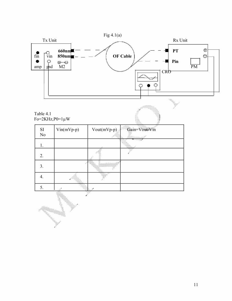
Fig 4.1(a)
Tx Unit Rx Unit
660nm PT
fin vin 850nm OF Cable
Pin
amp gnd M2 PM CRO
Table 4.1
Fo=2KHz,P0=1µW
SI Vin(mVp-p) Vout(mVp-p) Gain=Vout/Vin
No
1.
2.
3.
4.
5.
11
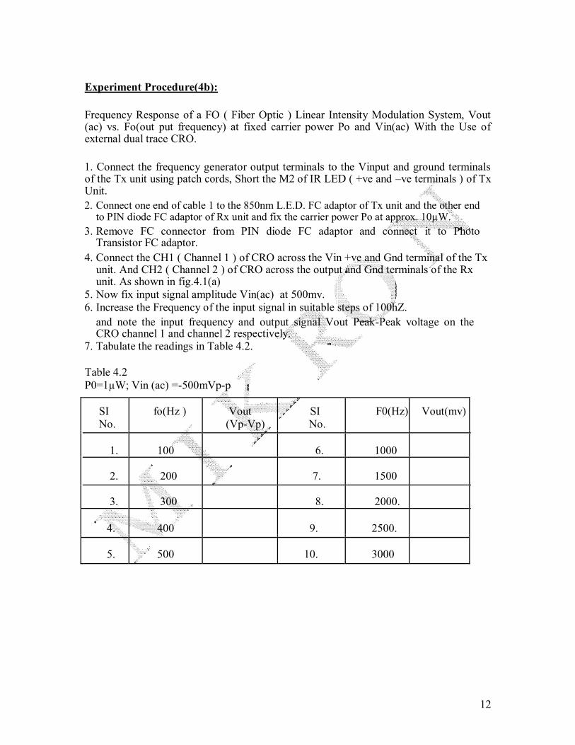
Experiment Procedure(4b):
Frequency Response of a FO ( Fiber Optic ) Linear Intensity Modulation System, Vout (ac) vs. Fo(out put frequency) at fixed carrier power Po and Vin(ac) With the Use of external dual trace CRO.
1. Connect the frequency generator output terminals to the Vinput and ground terminals of the Tx unit using patch cords, Short the M2 of IR LED ( +ve and –ve terminals ) of Tx Unit. 2. Connect one end of cable 1 to the 850nm L.E.D. FC adaptor of Tx unit and the other end
to PIN diode FC adaptor of Rx unit and fix the carrier power Po at approx. 10µW. 3. Remove FC connector from PIN diode FC adaptor and connect it to Photo
Transistor FC adaptor. 4. Connect the CH1 ( Channel 1 ) of CRO across the Vin +ve and Gnd terminal of the Tx
unit. And CH2 ( Channel 2 ) of CRO across the output and Gnd terminals of the Rx unit. As shown in fig.4.1(a)
5. Now fix input signal amplitude Vin(ac) at 500mv.
6. Increase the Frequency of the input signal in suitable steps of 100hZ.
and note the input frequency and output signal Vout Peak-Peak voltage on the CRO channel 1 and channel 2 respectively.
7. Tabulate the readings in Table 4.2.
Table 4.2
P0=1µW; Vin (ac) =-500mVp-p
SI fo(Hz ) Vout SI F0(Hz) Vout(mv)
No. (Vp-Vp) No.
1. 100 6. 1000
2. 200 7. 1500
3. 300 8. 2000.
4. 400 9. 2500.
5. 500 10. 3000
12
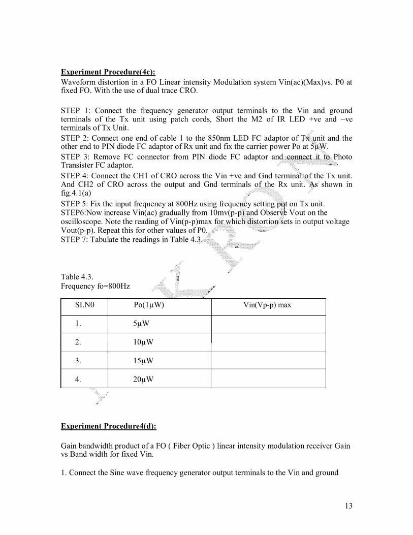
Experiment Procedure(4c): Waveform distortion in a FO Linear intensity Modulation system Vin(ac)(Max)vs. P0 at fixed FO. With the use of dual trace CRO.
STEP 1: Connect the frequency generator output terminals to the Vin and ground terminals of the Tx unit using patch cords, Short the M2 of IR LED +ve and –ve terminals of Tx Unit. STEP 2: Connect one end of cable 1 to the 850nm LED FC adaptor of Tx unit and the other end to PIN diode FC adaptor of Rx unit and fix the carrier power Po at 5µW. STEP 3: Remove FC connector from PIN diode FC adaptor and connect it to Photo Transister FC adaptor. STEP 4: Connect the CH1 of CRO across the Vin +ve and Gnd terminal of the Tx unit. And CH2 of CRO across the output and Gnd terminals of the Rx unit. As shown in fig.4.1(a) STEP 5: Fix the input frequency at 800Hz using frequency setting pot on Tx unit. STEP6:Now increase Vin(ac) gradually from 10mv(p-p) and Observe Vout on the oscilloscope. Note the reading of Vin(p-p)max for which distortion sets in output voltage Vout(p-p). Repeat this for other values of P0. STEP 7: Tabulate the readings in Table 4.3. Table 4.3.
Frequency fo=800Hz
SI.N0 Po(1µW) Vin(Vp-p) max
1. 5µW
2. 10µW
3. 15µW
4. 20µW
Experiment Procedure4(d):
Gain bandwidth product of a FO ( Fiber Optic ) linear intensity modulation receiver Gain vs Band width for fixed Vin.
1. Connect the Sine wave frequency generator output terminals to the Vin and ground
13
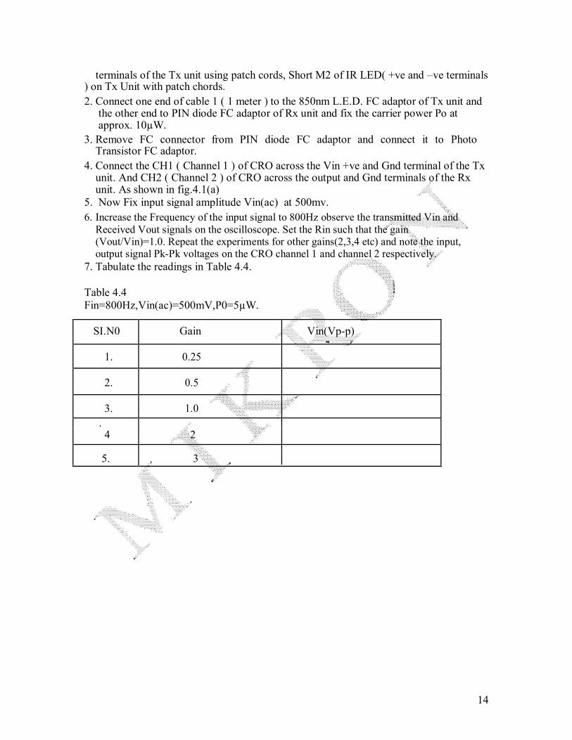
terminals of the Tx unit using patch cords, Short M2 of IR LED( +ve and –ve terminals
) on Tx Unit with patch chords. 2. Connect one end of cable 1 ( 1 meter ) to the 850nm L.E.D. FC adaptor of Tx unit and
the other end to PIN diode FC adaptor of Rx unit and fix the carrier power Po at approx. 10µW.
3. Remove FC connector from PIN diode FC adaptor and connect it to Photo Transistor FC adaptor.
4. Connect the CH1 ( Channel 1 ) of CRO across the Vin +ve and Gnd terminal of the Tx unit. And CH2 ( Channel 2 ) of CRO across the output and Gnd terminals of the Rx unit. As shown in fig.4.1(a)
5. Now Fix input signal amplitude Vin(ac) at 500mv. 6. Increase the Frequency of the input signal to 800Hz observe the transmitted Vin and
Received Vout signals on the oscilloscope. Set the Rin such that the gain (Vout/Vin)=1.0. Repeat the experiments for other gains(2,3,4 etc) and note the input, output signal Pk-Pk voltages on the CRO channel 1 and channel 2 respectively.
7. Tabulate the readings in Table 4.4.
Table 4.4
Fin=800Hz,Vin(ac)=500mV,P0=5µW.
SI.N0 Gain Vin(Vp-p)
1. 0.25
2. 0.5
3. 1.0
.
4 2
5. 3
14

EXPERIMENT 5: DETERMINATION OF NUMERICAL APERTURE OF OPTICAL FIBERS
Aim of the Experiment : The aim of the experiment is to determine the numerical aperture of the optical fibers available.
Theory: Numerical aperture of any optical system is a measure of how much light can be collected by the optical system. It is the product of refractive index of the incident medium and sine of the maximum ray angle.
NA=ni.sinӨmax ni for air is 1, Hence NA=
NOTE: In this particular experiment connections to Voltmeter (M1), Ammeter(M2),Signal generator are not required. Connect the circuit as mentioned below
Experiment Procedure:
The experimental set up for numerical aperture measurement system is as shown in below figure 5.1.
AC mains NA Jig
Tx unit
Set P0
Fig 5.1
1. Connect one end of the cable one to the 660nm L.E.D. FO connector of Tx Unit and
other end to the NA jig as shown in the above figure 5.1. 2. Plug the AC mains Turn the Po knob to clockwise direction to set maximum P0.
The light intensity should increase at the end of the fiber on the NA Jig.
3: Hold the white scale-screen, provided in the Kit vertically at a distance of 15mm(L) from the emitting fiber end and view the red spot on the screen (A dark room is necessary to facilitate a good contrast).
Now measure the maximum diameter(W) of the spot.
4. Compute NA from the formula NA = sinӨmax = W / (4L²+W²)½, Repeat the experiment at 10mm, 20mm an d 25mm distances and tabulate the readings in the table 5.1
15

Table 5.1
SI N0 L (mm) W(mm) NA Ө(degrees)
1.
2.
3.
4.
5.
Specifications of PMMA Fiber optic cable
16