AP StatisticsSemester One Review

Part 2Chapters 6-9

AP Statistics Topics

Describing Data

Producing Data

Probability

Statistical Inference

Chapter 6: Probability

This chapter introduced us to the basic ideas behind probability

and the study of randomness.We learned how to calculate and

interpret the probability of events in a number of different

situations.

ProbabilityProbability is a measurement of the likelihood of an event. It represents the proportion of times we’d expect to see an outcome in a long series of repetitions.

P(event) =# success

# possible

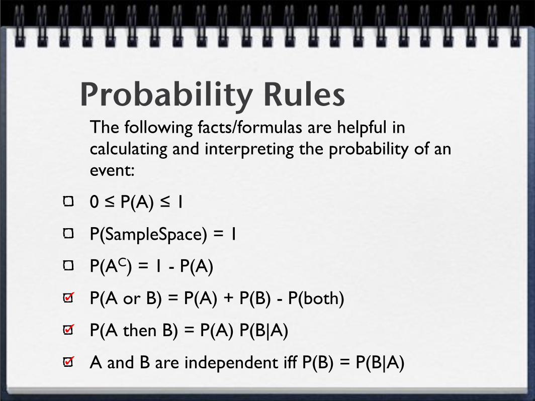
Probability RulesThe following facts/formulas are helpful in calculating and interpreting the probability of an event:

0 ! P(A) ! 1

P(SampleSpace) = 1

P(AC) = 1 - P(A)

P(A or B) = P(A) + P(B) - P(both)

P(A then B) = P(A) P(B|A)

A and B are independent iff P(B) = P(B|A)

Strategies

When calculating probabilities, it helps to consider the Sample Space.

List all outcomes if possible.

Draw a tree diagram or Venn diagram

Use the Multiplication Counting Principle

Sometimes it is easier to use common sense rather than memorizing formulas!

Chapter 7: Random Variables

This chapter introduced us to the concept of a random

variable.We learned how to describe an expected value and variability of

both discrete and continuous random variables.

Random Variable

A Random Variable, X, is a variable whose outcome is unpredictable in the short-term, but shows a predictable pattern in the long run.

Discrete vs. Continuous

Expected Value

The Expected Value, E(X)=µ, is the long-term average value of a Random Variable.

E(X) for a Discrete X

E(X) = µ = x ! p(x)"

X 1 5 20

P(x) 0.5 0.2 0.3

µ = 1(0.5) + 5(0.2) + 20(0.3)

= .5 +1+ 6

= 7.5

VarianceThe Variance, Var(X)= , is the amount of variability from µ that we expect to see in X.

The Standard Deviation of X,

Var(X) for a Discrete X X 1 5 20

P(x) 0.5 0.2 0.3

!2

! = Var(X)

Var(X) = !2= x " µ( )

2p(x)#

!2= (1" 7.5)

2(0.5) + (5 " 7.5)

2(0.2) + (20 " 7.5)

2(0.3)

= 21.125 +1.25 + 46.875

= 69.25

! = 69.25 = 8.32

Rules for Means and Variances

The following rules are helpful when working with Random Variables.

µa+bX = a + bµX

!2

a+bX = b2!2

X

µX ±Y

= µX± µ

Y

!2

X ±Y= !

2

X+!

2

Y

Chapter 8: Binomial and

Geometric Distributions

This chapter introduced us to the concept of the Binomial and

Geometric Settings.We learned how to calculate the likelihood of events occurring in

each of these settings.

Binomial SettingSome Random Variables are the result of events that have only two outcomes (success and failure). We define a Binomial Setting to have the following features

Two Outcomes - success/failure

Fixed number of trials - n

Independent trials

Equal P(success) for each trial

Binomial Probabilities

If X is B(n,p), the following formulas can be used to calculate the probabilities of events in X.

P(X = k) = nCk (p)k(1! p)

n! k

= binompdf (n, p,k)

P(X ! k) = binomcdf (n, p,k)

Normal ApproximationIf conditions are met, a binomial situation may be approximated by a normal distribution

If np"10 and n(1-p)"10, then B(n,p) ~ Normal

µX= np

!X= np(1" p)

Geometric SettingSome Random Variables are the result of events that have only two outcomes (success and failure), but have no fixed number of trials. We define a Geometric Setting to have the following features

Two Outcomes - success/failure

No Fixed number of trials

Independent trials

Equal P(success) for each trial

Geometric Probabilities

If X is Geometric, the following formulas can be used to calculate the probabilities of events in X.

µX=1

p

!X=

1" p

p2

P(X = k) = (1! p)k!1p

= geompdf (p,k)

P(X > k) = (1! p)k

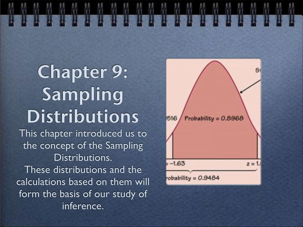
Chapter 9: Sampling

DistributionsThis chapter introduced us to the concept of the Sampling

Distributions.These distributions and the

calculations based on them will form the basis of our study of

inference.

Parameters and Statistics

Our goal in statistics to to gain information about the population by collecting data from a sample.

Parameter

Population Characteristic: µ, #

Statistic

Sample Characteristic: x-bar, p-hat

Sampling Distribution

When we take a sample, we are not guaranteed the statistic we measure is equal to the parameter in question. Further, repeated sampling may result in different statistic values.

Bias and Variability

Sampling DistributionsProportions

If the population proportion is # and

n#"10, n(1-#)"10 and pop>10n

Then the distribution of p-hat is approximately normal

Sampling DistributionsMeans

If the population mean is µ (and we know )

If the population is Normal OR n"30 (CLT)

Then the distribution of x-bar is approximately normal

!

Sampling DistributionsIf conditions are met, we know what the sampling distribution of a proportion or mean will look like.

Specifically, we know what sample value we’d expect to see and we know how close repeated samples should come to that expected value.

Since the distributions are normal, we can calculate the likelihood of observing specific sample values...

This is the basis for the inferential calculations we’ll study next semester!

Semester OneFinal Exam

50 QuestionsMultiple Choice

Chapters 1-9

Weds: Per 1,3,5Thurs: Per 2,4,6