appendix: useful concepts from circuit theory - springer978-1-4419-8957-4/1.pdf · appendix: useful...
TRANSCRIPT
Appendix: Useful Concepts from Circuit Theory
EDWIN R. LEWIS
1. Introduction
For understanding the physics of sound and the biophysics of acoustic sensors in animals, the concepts of impedance and admittance, impedance matching, transducer, transformer, passive and active, bidirectional coupling, and resonance are widely used. They all arise from the circuit-theory metamodel, which has been applied extensively in acoustics. As the name suggests, the circuit-theory metamodel provides recipes for constructing models. The example applications of the metamodel in this appendix involve a few elementary concepts from classical physics: the adiabatic gas law, Newton's laws of motion and of viscosity, and the definitions of work and of Gibbs free energy. They also involve a few elements of calculus and of the arithmetic of complex numbers. All of these should be familiar to modem biologists and clinicians. For further examples of the application of circuit concepts to acoustical theory and acoustical design, see Baranek (1954), Olsen (1957), or Morse (1981).
1.1 The Recipe Applied to an elementary physical process, such as sound conduction in a uniform medium, the appropriate recipe comprises the following steps:
1. Identify an entity (other than Gibbs free energy, see below) that is taken to be conserved and to move from place to place during the process.
2. Imagine the space in which the process occurs as being divided into such places (i.e., into places in which the conserved entity can accumulate).
3. Construct a map of the space (a circuit graph) by drawing a node (e.g., a small dot) for each place.
4. Designate one place as the reference or ground place for the process. 5. Assign the label "0" to the node representing the ground place. 6. Assign a unique, nonzero real integer (i) to each of the other nodes in the
graph. 7. Define the potential difference between each place (i) and the ground place
(0) to be F;o, the corresponding Gibbs potential for the conserved entity
369
370 E.R. Lewis
(change in Gibbs free energy of the system per unit of conserved entity moved from place 0 to place i).
8. From basic physical principles (or by measurement), determine the relationship between the amount, Q;, of conserved entity accumulated at place i and the potential F;o.
9. From basic physical principles (or by measurement), determine the relationship between potential difference F;j between each pair of neighboring places and the flow lij of conserved entity between those places.
The Gibbs free energy of a system is defined as the total work available from the system less that portion of the work that must be done against the atmosphere. For one-dimensional motion from point a to point b, the work (Wah) done by the system is defined by the expression Wah = Jj~a fix)dx where fix) is the force applied by the system to the object on which the work is being done. The force is taken to be positive if it is applied in the direction in which the values of x increase; otherwise it is taken to be negative. For tables of Gibbs potentials for various conserved entities, see Lewis (1996).
1.2 Example: An Acoustic Circuit Model As an example application of the recipe, consider the conduction of sound, axially, through an air-filled cylindrical tube with rigid walls. In that case, one might identify the conserved entity as the air molecules that move from place to place along the tube. As air molecules accumulate at a given place, the pressure at that place increases. Assuming that the air pressure outside the tube is uniform and equal to atmospheric pressure, it is convenient to take that place (the outside of the tube) to be the reference place. The SI unit for number of air molecules is 1.0 mol. Therefore, the SI unit for the flow of air molecules will be 1.0 molls; and the SI unit for the Gibbs potential will be 1.0 joule/mol. If one takes Pi to be the absolute pressure at place i along the inside of the tube (SI unit 1.0 ntlm2 = 1.0 Pa) and Po to be the absolute atmospheric pressure, then the sound pressure (l1pJ at place i will be the difference between those two pressures:
(1)
Acousticians usually assume that the processes involved in sound propagation are adiabatic and that sound pressures are exceedingly small in comparison to atmospheric pressure:
I1n. _'1'_' «1.0 (2) Po
The Gibbs potential difference, F iO' between place i and the reference place is given by:
F = f).pi iO (3)
Co
Appendix: Useful Concepts from Circuit Theory 371
where Co is the resting concentration of air molecules (SI unit = 1.0 moUm3).
(4)
where no is the resting number of air molecules at place i, and Vo is the volume of place i (assumed to be constant). The resting absolute pressure at place i is taken to be Po.
Equation 3 for the Gibbs potential can be derived easily from the equation for work. Invoking the adiabatic gas law, one can derive the relationship between the Gibbs potential at place i and the excess number of air molecules at place i, b.ni , where
(5)
ni being the total number of air molecules at place i. For !1p/Po exceedingly small, the adiabatic gas law can be stated as follows:
(6)
where y is 1.4, the ratio of specific heat of air at constant pressure to that at constant volume. From this,
F = !1pi = Wo A.. iO ill!; (7)
Co cono
In the circuit-theory metamodel, this is a capacitive relationship. The general constitutive relationship for a linear, shunt capacity at place i in any circuit is
F = Qi iO Ci
(8)
where the parameter Ci often is called the capacitance or compliance. In this case, Qi' the accumulation of conserved entity at place i, is taken to be to be f).ni'
(9)
Dividing the cylindrical tube axially into a large number of segments of equal volume, Vo, brings the first eight steps of the metamodel recipe to completion. For the ninth step one might assume that the acoustic frequencies are sufficiently high to preclude significant propagation of drag effects from the wall of the cylinder into the mainstream of axial air flow. In other words, one might ignore the effects of viscosity (see subsection 8.2). Absent viscosity, the axial flow of air molecules would be limited only by inertia. Lumping the total mass of air molecules at a single place, and invoking Newton's second law of motion, one has the following relationship for the flow, Jij' of molecules from place i to its neighboring place, j:

372 E.R. Lewis
dIij = A5C5 F dt VoPo IJ
(10)
where t is time, Po is the resting density of the air (SI unit equal 1.0 kg/m3),
and Ao is the luminal area of the cylindrical tube. In the circuit-theory metamodel, this is an inertial relationship. The general constitutive relationship for a linear, series inertia between place i and j in any circuit is
(11)
where the parameter Iij often is called the inertia or inertance. In this case,
2. Derivation of an Acoustic Wave Equation from the Circuit Model
(12)
Having thus completed the circuit model, one now can extract from it an equation describing sound conduction through the tube. This normally is accomplished by writing explicit expressions for the conservation of (conserved) entity at node i and the conservation of energy in the vicinity of node i, and then incorporating the constitutive relations obtained in steps 8 and 9 of the metamodel recipe. Let node i have two neighbors, node h on its left and node j on its right. Conservation of air molecules requires that
From Equation 8 one notes that
dQi = CdFiO dt I dt
Therefore,
Conservation of energy requires that
Therefore,
dJ Fo - Fo = /---3.
I J IJ dt
(13)
(14)
(15)
(16)
(17)

Appendix: Useful Concepts from Circuit Theory 373
2.1 Translation to a Transmission-Line Model In the manner of Lord Rayleigh, one can simplify further analysis by taking the limit of each side of Equations 15 and 17 as one allows the number of places represented in the model to become infinite and the extent of each place infinitesimal. Each place represented in the circuit model has length Lo given by
Vo L=o Ao
(18)
Dividing Ci and Ii by Lo, one has the capacitance and inertance per unit length of the uniform, air-filled tube:
(19)
Now, let x be the distance along the tube and let the length of each place be Llx. One can rewrite Equations 15 and 17 as follows:
~ dF -AJ = l· -- J = C Llx-
hI IJ dt
~ dJ -M' = Fo - Fo = I Llx-
I ] dt (20)
Dividing each side of each equation by Llx and taking the limit as Llx approaches zero, one has
d [Ill] ~ d - -lex t) = lim -- = C-F(x t) dx' LIx->O L1 x dt'
d [L1F] ~d --F(x t) = lim -- = 1-l(x t) dx' LIx->O L1x dt' (21)
These are the classic transmission-line equations, variations of which have been used widely in neurobiology. Traditionally, they are written in a more general form:
dF - - zJ dx dJ - - yF dx
(22)
where z is the series impedance per unit length of the transmission line, and y is the shunt admittance per unit length; and F and J are linear transforms of F and l. Although the notions of impedance and admittance are treated here in a general sense, when they involve time derivatives (as they do here), circuit theorists normally apply them to one of two carefully restricted situations: (1)
374 E.R. Lewis
sinusoidal steady state (a pure tone has been applied for an indefinitely long time); or (2) zero state (a temporal waveform is applied; at the instant before it begins, all Fs and is in the circuit model are equal to zero). For sinusoidal steady state, circuit theorists traditionally use the phasor transform; for zero state they traditionally use the Laplace transform. Yielding results interpretable directly in terms of frequency, the former is widely used in classical acoustics texts.
2.2 Derivation of the Phasor Transform The definition of the phasor transform is based on the presumption that exponentiation of an imaginary number, such as ix (where i is the square root of -1), obeys the same rules as exponentiation of a real number (such as x).
Specifically, it is presumed that eix can be evaluated by substituting ix for x in the Maclaurin series for ex. In that case,
eix = cos x + i sin x
and
cos x = Re{ eix}
where Re{z} is the real part of the complex number, z:
z = a + ib i = r=T
~
Re{z} = a
(23)
(24)
(25)
The phasor transform applies to sinusoidal steady state, with the radial frequency of the sinusoid being w (SI unit = 1.0 rad/s).
w = 2rtf (26)
where f is the conventional frequency (unit = 1.0 Hz). One can represent the phasor transformation as follows:
H(w) = <I>{H(t)} H(t) = <I>-IH(w) (27)
where the function of frequency, H( w), is the phasor transform of the time function H(t). The transform is defined by its inverse
H(t) = <I>-I{H(w)} ~ Re[H(wkWt] (28)
Combining this with Equations 23-25, one finds the following basic transform pairs:
<I> { coswt} = 1 <1>-1 {1} = cos wt <I>{A cos(wt + a,)} = Aeiu = A cos a, + iA sin a, <I>-I{AeiU } = <1>-1 {A cos a, + iA sin a,} = A cos(wt + a,) (29)

Appendix: Useful Concepts from Circuit Theory 375
Notice that
(30)
Thus, mUltiplying the phasor transform of a sinusoidal function of time (of any amplitude and phase) by the factor Aeia corresponds to two mathematical operations on the function itself: (1) multiplying the amplitude of the function by the factor A, and (2) adding a. radians to the phase of the function. Taking the first derivative of any sinusoidal function of time can be described in terms of the same two operations: (1) the amplitude of the function is multiplied by w, and (2) rrJ2 radians (90 degrees) are added to the phase of the function. Thus,
<I> { ~~t)} = wei~H(w) (31)
Applying Equation 23, one has Jt
e'2 = i
<1>( ~~t)) = iwH(w) (32)
2.3 Phasor Transform of the Transmission-Line Model Based on Equation 32, one can write the transformed version of Equation 21 as follows:
d A
dx F(x,w) = -iwIJ(x,w)
d A
dxJ(x,w) = -iwCF(x,w) (33)
Thus, for the transmission-line model (Eq. 22), under sinusoidal steady state at radial frequency w, z and y would be written as follows:
z = i wi y = i we (34)
To simplify notation in transformed equations, w often is omitted in the arguments of the dependent variables J and F. For z and y both independent of x, as they are taken to be in this case, the spatial solutions to these equations usually are written in one of two forms: Form 1
J(x) = FJx) + F.(x)
JAx) = YoFAx)
FAx) = ZJAx)
J(x) = JAx) - J.(x)
J.(x) = YoF.(x)
F.(x) = ZoJ.(x)
z.~;,~~ F.(x) = Fr(O)e fzYx (35)
376 E.R. Lewis
Form 2
F(x) = F(O) cosh([zY x) - ZoI(O) sinh([zY x)
J(x) = J(O) cosh([zY x) - YoF(O)sinh([zY x)
~ 2.4 Forward and Reverse Waves
(36)
Define the forward direction for the transmission line as the direction of increasing values of x. In the first form, Flx) and Jlx) are interpreted as being the potential and flow components of a wave traveling in the forward direction; F,(x) and Jr(x) are interpreted as the components of a wave traveling in the reverse direction. At any instant, the product Fix)If(x) of the corresponding time functions is the rate at which the forward wave carries Gibbs free energy (in the forward direction) past location x, and the product Flx)I,(x) is the rate at which the reverse wave carries Gibbs free energy past x (in the reverse direction).
2.4.1 Speed of Sound and Characteristic Impedance
For the simple transmission-line model under consideration here, z is purely inertial and y is purely capacitive. The wave components in form 1 of the solution become
Flx) = FlO)e- iiicwx
F,(x) = FlO)e+ iiicwx (37)
Both components are sinusoids, radial frequency w. For the forward component, the phase at distance x from the origin lags that at the origin by an amount that is directly proportional to x. That is the behavior of a wave traveling at constant speed in the direction of increasing x (the forward direction). For the reverse component, the phase at distance x leads that at the origin by an amount proportional to x. That is the behavior of a wave traveling at constant speed in the direction of decreasing x (the reverse direction). For both components, the amplitude is independent of x. The speed, <1>, of the wave is the same in both cases. The solution is valid for all frequencies, so one can generalize it to waves of arbitrary shape that travel at constant speed without changing shape:
Ff (x,t) = Ff (O,t - ~) If (x,t) = YoFf (x,t)
F,(x,t) = Fr (O,t + ~) Ir (x,t) = YOFr (x,t) (38)
(39)

Appendix: Useful Concepts from Circuit Theory 377
1 /i:PO ~ - .-- jfc- Po (40)
The parameter Zo, usually called the characteristic impedance, is a positive real number in this case. For sinusoidal steady state this implies that at each place (each value of x) along the acoustic path, Ff and Jf are perfectly in phase with one another, as are Fr and Jr' The relationship between Zo and the physical parameters of the system and its SI unit both depend on the choice one made at step 1 of the metamodel recipe. If one carries out the model construction correctly, however, the wave speed will be independent of that choice.
3. Alternative Formulations of the Circuit Model
Instead of taking the number of air molecules as the conserved entity, one might have taken their mass. Assuming that the density changes induced in the air by the propagating sound wave are negligible (the analysis in section 2 was based on the same assumption), acousticians often use fluid volume as the conserved entity (as a surrogate for mass). Sometimes mass itself is used. All of these choices lead to equivalent formulations and moving from one to another requires only the application of appropriate multiplicative factors. The SI unit of impedance for each choice of conserved entity is easily determined. If the selected entity were apples, with an SI unit of 1.0 apple, then the SI unit of flow would be 1.0 apple/s, and the SI unit of Gibbs potential would be 1.0 joule/apple. The SI unit of impedance would be that of Gibbs potential divided by flow-1.0 joule s per apple2. For the acousticians' choice of volume, the SI unit of conserved entity is 1.0 m3. The SI unit of impedance becomes 1.0 joule s per m6•
For the choice made at the beginning of section 1.2 (SI unit of conserved entity = 1.0 mol), the SI unit of impedance is 1.0 joule s/moF.
3.1 Conventional Acousticians' Formulation To obtain the acousticians' J (SI unit 1.0 m3/s), one divides the J of section 2 (SI unit 1.0 molls) by CO (SI unit 1.0 mollm3). To obtain the acousticians' F (SI unit 1.0 joule/m3), one multiplies the F of section 2 (SI unit 1.0 joule/mol) by Co. When these changes are made, the inertance and compliance per unit length become.
A Ao c='YPo
A Po 1=-
Ao
and the characteristic impedance, Zo, becomes
(41)

378 E.R. Lewis
z = /'fPoPo o A
o (42)
Recognizing "{Po as the adiabatic bulk modulus of an ideal gas at pressure Po, one can translate Equations 40 and 42 into general expressions for compressional (longitudinal) acoustic waves in fluids:
(43)
(44)
where ~ is the speed of sound in the fluid; 20 is the characteristic acoustic impedance of the fluid; EB is the fluid's adiabatic bulk modulus; p is its density, and Ao is the cross-sectional area of the acoustic path (the luminal area of the cylindrical tube in the system being modeled here). Once again, these expressions were based on the presumption that changes in the fluid density, p, produced by the waves are exceedingly small.
3.2 Modeling Perspective Following a path already well established by physicists, with the circuit-theory metamodel as a guide, the development to this point has combined that presumption (exceedingly small changes in fluid density) with two conservation principles (energy is conserved, matter is conserved) and with two of the empiricallinear laws of physics (the adiabatic form of the ideal gas law-translated to a form of Hooke's law, and Newton's second law of motion) to reconstruct a theory of sound propagation. With the theory constructed, mathematics was used to determine where that combination of presumptions, principles, and empirical laws would lead. What the analysis showed was that the local elastic and inertial properties of fluids (gases and liquids) should combine to allow spatially extensive sound propagation. It also showed that if that were the case, then the speed of propagation should be related to the elastic and inertial parameters (adiabatic bulk modulus and density) in the specific manner described in Equation 43. In fact, the derived relationship (Eq. 43) predicts extremely well the actual speeds of sound in fluids (gases and liquids). This should bolster one's faith not only in the specific theory, but also in the modeling process itself. It follows the pattern established by Isaac Newton and practiced successfully by celebrated physical scientists over and over again since his time. Newton com-
Appendix: Useful Concepts from Circuit Theory 379
bined a presumption about gravity with a conservation law (momentum is conserved) and with his second law of motion to construct a theory of planetary motion. He used mathematics to see where that theory would lead. Where it led was directly to Kepler's laws, which are empirical descriptions of the actual motions of planets. Recently, writing about Newton's Principia, where this theory and its analysis first were published, a noted physicist said that the astounding conclusion one would draw from the work is the fact that nature obeys the laws of mathematics. I would put it differently. Physical nature appears to behave in an astoundingly consistent manner. In mathematics, mankind has invented tools that allow concise and precise statements of apparently consistent local behaviors (e.g., empirically derived laws), tools (such as the circuittheory metamodel) that allow those statements to be combined to construct theories of spatially (in its general sense) more extensive behaviors, and tools to derive from those theories their predictions. The fact that the predicted behaviors so often match, extremely well, observed behaviors, is attributable to physical nature's consistency.
Returning to the metamodel and to the first step in the recipe, one can see that momentum (Newton's choice) is a particularly interesting alternative to be taken as the conserved entity. Newton's second law equates the force two particles exert on one another to the flow of momentum between them, and (for nonrelativistic systems) the Gibbs potential difference for that momentum flow is the difference between the particles' velocities. When one chooses fluid mass, fluid volume, or number of fluid molecules as the conserved entity, J is proportional to velocity and F is proportional to force. With momentum as the choice, F is proportional to velocity, J is proportional to force. This is an example of the celebrated duality that arises in the circuit-theory metamodel.
4. Generalization to Plane Waves
As long as the consequences of viscosity were negligible, the presence of the rigid cylindrical walls posited in the previous subsections had only one effect on the propagation of sound waves through the fluid inside the cylinder. It forced that propagation to be axial. The transmission-line equations derived for the fluid in the cylinder would apply perfectly well to propagation of a plane wave through any cross-sectional area Ao, normal to the direction of propagation, in an unbounded fluid medium (e.g., air or water). The propagation speed derived for the waves confined to the fluid in the cylinder is the same as it would have been for unconfined plane waves in the same fluid. The expression for characteristic impedance (Eq. 44) would apply to an interface, normal to the direction of propagation, with cross-sectional area Ao. Viewed locally, propagating sound waves usually approximate plane waves, making Equation 44 and its antecedents very general. In an unbounded fluid, however, the propagation of sound waves is not confined to a single coordinate. A local volume in such a fluid could have sound waves impinging upon it from all directions at once.
380 E.R. Lewis
The instantaneous local sound-pressure component of each of these waves is a scalar, and the pressures from all of the waves together would sum to a single value. The local volume flow component of each wave will now be a vector (having an amplitude and a direction), and the flows from all of the waves would sum vectorially, at any given instant (t), to a single amplitude and direction. For a sound wave from a given direction, the local flow of Gibbs free energy through a cross-sectional area Ao would be given by the product of the local flow vector (J(t» for that wave and the corresponding local Gibbs potential (F(t» for that wave. Notice that the product itself now is a vector, with amplitude and direction. The direction of the vector is the direction of energy flow. Notice that it is the same as the direction of J(t) whenever F(t) is positive. The crosssectional area, Ao, would be taken in a plane normal to the direction of energy flow.
4.1 Particle Velocity Noting that J(t) for a uniform plane wave would be directly proportional to Ao, one can normalize it to form another variable-flow density ({l(t».
(45)
When J is volume flow (the acousticians' choice, SI unit = 1.0 m3/s), {l is the sound-induced component of the velocity of the fluid (SI unit = 1.0 mls). In that case, it traditionally is labeled the particle velocity. F, in that case (volume taken to be the conserved entity), is the local sound pressure. Whatever the choice of conserved entity, the instantaneous product F{l will be a vector whose amplitude is the instantaneous flow of Gibbs free energy per unit area (SI unit = 1.0 W/m2), and whose direction is the direction of that energy flow.
It is interesting to contemplate the vector sum of particle velocities of several unrelated sound waves impinging on a small local volume from different directions in an extended fluid. The local sound pressure would vary in time much as it might for a plane wave. The particle-velocity vector, on the other hand, would vary not only in amplitude, but also in direction. Try to imagine the computational task one would face trying to reconstruct the original sound waves from the combination of that scalar function, F(t), and that vector function, {let).
4.2 Particle Displacements For an acoustical sine wave, the local particle velocity is a sinusoidal function of time, as is the corresponding local particle displacement, 8(x,t). One can compute the amplitude, D(x), of the latter directly from the amplitude, B(x), of the former:
Appendix: Useful Concepts from Circuit Theory 381
{}(x,t) = B(x)cos(wt)
f B(x)sin(wt) 8(x,t) = D(x)sin(wt) = {}(x,t)dt = ----.:..-.:'-----.:..-.:
W
D(x) = B(x) (46) w
This, in tum, can be related to the local peak sound pressure, f1p(x), through the characteristic impedance:
F(x,t) = l\p(x)cos(wt)
{}(x,t) = J(x,t) = F(x,t) = F:::J Ao AaZo ~EBP
B(x) = ~ ,jEBP
D(x) = l\p(x) wJEBP
~ EB ,jEBP = p~ =--~
(47)
In water, p is approximately 103 kg/m3 and ~ is approximately 1.5 X 10³ mis, making p~ approximatelly 1.5 X 10⁶ kg/m2s. Standard pressure of 1.0 atm is defined to be 101,325 Pa. The velocity of sound in dry air at 1.0 atm and 200e is approximately 340 mls. Therefore, for dry air at 1.0 atm and 20oe, EB/~ (which is 1.4pJ~) is approximately 400 kg/m2s. For a given sound pressure, this means that the peak local particle displacement in air will be almost 4000 times as great as it is in water.
For a 100-Hz tone with a peak sound pressure of 1.0 Pa (the upper end of the usual sound intensity range), for example, the peak local particle displacement in water would be approximately 10 nm. In air, it would be 40 /.-lm. For I-kHz tones, those particle displacements would be 1 nm and 4 /.-lm, respectively, and for 10 kHz they would be 0.1 nm and 0.4 /.-lm. At the nominal threshold level for human hearing (0.00003 Pa) at 1.0 kHz, they would be 0.03 pm and 0.12 nm. If an evolving animal were able to couple a strain-sensitive device (neural transducer) directly to a flexible structure (e.g., a cuticular sensillum, an antenna, hair) projecting into the air, then a sense of hearing could evolve based on direct coupling of particle-velocity to that structure. One would guess that such a sense would be limited to low-frequency, high-intensity sounds. For a strain-sensitive device (e.g., a bundle of stereovilli) projected into water, on the other hand, an evolving sense of hearing based on direct coupling of particle velocity to that device would be much more limited (4,000 times less effective at every frequency, every intensity). For such a device, one might expect evolution to have incorporated auxiliary structures to increase the displacement of the strain-sensor well beyond the particle displacement of the acoustic wave in the medium. For detection of airborne sound, such auxiliary structures also would have to include a mechanism for transferring acoustic energy from the

382 E.R. Lewis
air to the strain sensor. In the language of the circuit-theory metamodel, the latter would be a transducer, the former a transformer or an amplifier.
5. Passive Transducers
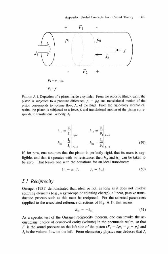
In the basic circuit model, one tracks the flow of a single entity from place to place. By taking F to be the Gibbs potential for that entity, one is able to track the flow of Gibbs free energy as well. The conserved entity will be confined to a particular realm. Air molecules, for example, are confined to the volume containing the air, which one might label the pneumatic realm. The Gibbs free energy (acoustic energy) that they carry, on the other hand, can be transferred in and out of that realm. In the circuit-theory metamodel, a device that transfers energy from one physical realm to another is a transducer. A piston can be modeled as such a device. It can translate sound pressure, FI , and flow of air molecules, 11, in a pneumatic realm to a Gibbs potential, F2, and flow, 12, appropriate to a translational rigid-body mechanical realm, and vice versa. In doing so, it carries Gibbs free energy back and forth between those two realms. For a rigid-body mechanical realm, there are two common choices for conserved entity: (1) the shapes of the rigid elements, or (2) momentum. In rigid-body mechanics, it is convenient to treat each of the orthogonal directions of translational and rotational motion as a separate realm. For the piston, the motion of interest is axial (translational motion perpendicular to the face of the piston). Following standard engineering practice, one would select axial displacement as the conserved entity (as a surrogate for shape, displacement is conserved as it passes through an element whose shape does not change). The SI unit of displacement is 1.0 m. The flow, 12, becomes axial velocity (SI unit = 1.0 mls); and the Gibbs potential, F2, becomes force (SI unit = 1.0 joule/m). The directions assigned in Fig. A.1 are the conventional associated reference directions for the circuit-theory construction known as a two-port element. When FI is positive, it tends to push the piston to the right, the direction assigned to positive values of 11, When F2 is positive, it tends to push the piston to the left, the direction assigned to positive values of 12,
Constitutive relationships for the piston can be expressed conveniently in the following form:
FI = hllJI + h12F2 J2 = h21JI + h22F2 (48)
where the parameters h12 and h21 are transfer relationships; hll is an impedance (ratio of a Gibbs potential to the corresponding flow); and h22 is an admittance (ratio of a flow to the corresponding Gibbs potential). One estimates these parameters individually (by measurement or by invoking simple physics) from the following equations:
Appendix: Useful Concepts from Circuit Theory 383
PI PO
.. ~ .............. .
J2
F2 +
FIGURE A.I. Depiction of a piston inside a cylinder. From the acoustic (fluid) realm, the piston is subjected to a pressure difference, PI - Po; and translational motion of the piston corresponds to volume flow, II' of the fluid. From the rigid-body mechanical realm, the piston is subjected to a force, 1, and translational motion of the piston corresponds to translational velocity, 12•
hll = ~: I F2~O F'I h12 =-
F2 lt~O
h21 = ~ IF2~o h = J2
1 (49) 22 F
2 JI~O
If, for now, one assumes that the piston is perfectly rigid, that its mass is negligible, and that it operates with no resistance, then hll and h22 can be taken to be zero. That leaves one with the equations for an ideal transducer:
(50)
5.1 Reciprocity Onsager (1931) demonstrated that, ideal or not, as long as it does not involve spinning elements (e.g., a gyroscope or spinning charge), a linear, passive transduction process such as this must be reciprocal. For the selected parameters (applied to the associated reference directions of Fig. A.I), that means
(51)
As a specific test of the Onsager reciprocity theorem, one can invoke the acousticians' choice of conserved entity (volume) in the pneumatic realm, so that F, is the sound pressure on the left side of the piston (FI = !J.PI = PI - Po) and J1 is the volume flow on the left. From elementary physics one deduces that J I

384 E.R. Lewis
will be zero when FI (the net pressure pushing from the left) times the luminal area, Ao, is equal to the force pushing from the right. Therefore,
(52)
When there is no force from the right (F2 is zero), so that the piston could not be deformed even if it were not perfectly rigid, then from elementary geometry one knows that the (rightward) volume flow into the piston, f l , must equal the luminal area, Ao' times the rightward velocity of the piston. Therefore,
(53)
and h12 = - h2" as the Onsager theorem says it must.
5.2 Bidirectionality and Its Implications: Driving-Point Impedance Reciprocity implies bidirectionality (Gibbs free energy can be transferred in both directions across the transducer), which in tum implies that what happens in either of the physical realms connected to a transducer will affect what happens in the other physical realm. This implication becomes explicit in the expressions for driving-point impedance or admittance. Imagine an acoustic source on the left side of the piston, and mechanical impedance (e.g., a combination of masses, springs, and dashpots) on the right, as in Fig. A.2. Here, the mechanical impedance is designated simply ZM' For the general linear situation, one would have
(54)
.---Zdp(l) , ...... ZM ------!"
I " I ______ ~ ...
'--
Acoustic source
FIGURE A.2. Depiction of an acoustic source connected to a mechanical load (impedance ~) through a piston. The resulting pneumatic impedance, 2dp(l), faced by the source depends on both 2M and the properties of the piston (see text).
Appendix: Useful Concepts from Circuit Theory 385
from which
Z (1) = FI = h _ hl2h21 dp JI II h22 + 1I~ (55)
where ZdP(1) is the (driving-point) impedance that the acoustic source faces as it drives the transducer from the pneumatic realm. It should not be surprising that Zdp(1) depends strongly on what is connected to the transducer in the other realm (i.e., on ~). For this passive transducer (which has no spinning elements), with hll and h22 both equal zero,
(56)
Note that with the current choices of conserved entities (volume in the pneumatic realm, axial displacement in the rigid-body mechanical realm) the SI unit of ZdP(1) is 1.0 joule s per m6 and that of ~ is 1.0 joule s per m2• The factor lIA5 translates the rigid-body mechanical impedance, ~, into the pneumatic impedance, ZdP(l).
6. Terminal Impedances and Reflected Waves
Imagine the piston with its very short cylinder (luminal area Ao) connected to the end (x = L) of an air-filled tube (also with luminal area Ao). ZdP(1) now forms what is known as a terminal impedance for the acoustic path through the air in the tube. Applying form 1 of the transmission-line equation (Eq. 35), one has
FI = FAL) + Fr(L) = Zdp(1)JI JI = JAL) - J,(L)
FAL) = ZJAL) F,(L) = ZJr(L) (57)
where FI and JI are the sound pressure and volume flow applied to the piston by the air in the tube; Zo is the characteristic impedance of the acoustic path through the air in the tube. From Equation 57 one can derive the reflection coefficient Fr(L)IFAL) of the air-transducer interface:
S = ZdP(l) - Zo
Ff ZdP(1) + Zo (58)
If the goal is to maximize the transfer of Gibbs free energy from the pneumatic realm (acoustic energy) to the rigid-body mechanical realm (mechanical energy), then one wants to minimize the amplitude of the reflected wave, Fr. It is clear from Equation 58 that Fr will be reduced to zero if ZdP(1) = ZOo In other words, there will be no reflection if the acoustic path is terminated with an impedance equal to the characteristic impedance of the path. If that is not so, one often can make it so by inserting an appropriate passive transformer on one side or the other of the transducer (the piston).

386 E.R. Lewis
6.1 Transformers and Impedance Matching
The simplest passive transformers are constructed as a cascade of two passive transducers connected back to back. Consider the system depicted in Figure A.3. Here are two rigid-walled cylindrical tubes containing different fluids. Between the two fluids is a cascade of two pistons connected back to back in a translational rigid-body mechanical realm. Being reversed, the second piston is represented by a two-port model in which FI is force, 11 is rightward translational (axial) velocity, F2 is pressure, and 12 is leftward volume flow. In that case, if one assumes as before that the piston is perfectly rigid, that its mass is negligible, and that it operates with no resistance,
h11 = 0 (59)
Applying Equation 55 to this situation (~ becomes Z02)' one finds that the mechanical driving-point impedance at the left side of the second piston is
(60)
Applying the same equation to the first piston (the piston is not reversed, ~ becomes ZdP(P2», one finds that the driving-point impedance at the left side of the complete transformer is
(61)
To avoid reflections of sound waves as they pass from fluid 1 to fluid 2 through the transformer formed by the pistons, one requires
A2 2
A 2 Z02 = ZOI 1
(62)
Substituting the expression for Zo from Equation 44, one can restate this requirement in terms of the densities and adiabatic bulk moduli of the two fluids:
(63)
r--
ZdP(P2)Q r--
ZdP(Pl)Q Z02
ZOI ~
~
FIGURE A.3. Depiction of an acoustic transfonner comprising back-to-back pistons rigidly connected in the rigid-body mechanical realm. The transfonner couples an acoustic medium with characteristic impedance ZOI to one with characteristic impedance Zoo.

Appendix: Useful Concepts from Circuit Theory 387
The symmetry of this relationship implies that when it is true, sound waves pass through the transformer in either direction without reflection.
Equation 61 is a form of the classic transformer equation, 't being the transformer ratio. By adjusting 't (the ratio of piston areas), one could, in principle, transform any real-valued impedance (Z02) to match any other real-valued impedance (e.g., ZOI)' A mechanical transformer in which 't is less than 1.0 is said to provide mechanical advantage. The passive device that does so comprises either a single pair of back-to-back passive transducers (a simple machine), or multiple pairs of such transducers (a compound machine). In addition to pistons and their relatives (including flexible diaphragms), the repertoire of passive mechanical transducers includes the wheel (transfers free energy between translational and rotational realms), which is the basis of gear systems and pulley systems, and the semilever-a rigid bar between a fulcrum and a point of applied force (also transfers free energy between translational and rotational realms), which is the basis of lever systems. For gear or pulley systems, 't is the ratio of wheel (e.g., pulley or gear) radii; for lever systems it is the ratio of semilever lengths.
7. Driving-Point Impedance of a Terminated Acoustic Path
In the previous subsection, the piston was modeled as a circuit element with two distinct ports: port 1 facing the pneumatic realm, and port 2 facing the rigidbody mechanical realm. The same sort of model can be useful as well in a single realm. Suppose the length of a fluid-filled, rigid-walled cylindrical tube were L. If one were concerned only with the acoustic variables (Fs and Js) at the ends of the tube, one could translate the transmission-line model (Eq. 36) to a two-port model, one port representing one end of the tube, the other port representing the other end. For that purpose, it is useful to use the two-port impedance (z) parameters instead of the two-port hybrid (h) parameters:
(64)
where FI and JI in Equation 64 correspond to F(O) and J(O), respectively, in Equation 36; F2 and J2 in Equation 64 correspond to F(x) and J(x) in Equation 36 when x is set equal to L. The corresponding z parameters are derived as follows:
Zl1 = ~: 112=0 = ~~; I J(L)=O
J2 = J(L) = 0 = J(O)cosh(m L) - YoF(O)sinh(m L)
cosh(m L) z - Z ----';:=--11 - °sinh(m L)
Z21 = ~Jl=O = ~~;IJ(O)=o sinh~ L) (65)

388 E.R. Lewis
and, by symmetry, Z22 = Zll' Z21 = Zl2' The equality of Z12 and Z21 (or, equivalently, h12 = -h21 ) also is stated in a general reciprocity theorem that applies to all passive, linear circuit models in which rotation (sometimes called gyration) is not represented. Proof of the theorem can be found in standard circuit-theory texts. For the Z parameter set, Equation 55 becomes
(66)
where ZL is the (load) impedance connected to port 2. In this case, ZL is the external impedance that the sound wave encounters as it reaches the far end of the tube (where x = L). Combining Equations 65 and 66, one finds the general expression for the driving-point impedance that an acoustic wave would face as it enters the tube (at x = 0).
ZL cosh(/zy L) + Zo sinh(/zy L) Zd=ZO C r-
p Zo cosh(,lzy L) + ZL sinh(~zy L) (67)
Notice that if ZL equals Zo, so that there is no reflected wave, then Zdp also equals ZOo What Equation 67 describes is the impact of the reflected wave on the driving point impedance when ZL does not equal ZOo For the fluid-filled tube, with a steady tone (frequency wo = 2rtfo) applied to the near end (x = 0), the driving-point impedance becomes
(68)
where A is the wavelength of the tone in the fluid (e.g., in air or in water):
(69)
As the frequency of the tone increases and VA shifts from 0 to 0.25, Zdp will shift from ZL to Z2r/ZL' For intermediate values of VA, the values of Zdp will be complex numbers, implying phase differences between Fl and fl' The size of the phase difference will depend strongly on the frequency of the tone.
7.1 The Significance of Phase Difference: Passivity Constraint To understand the significance of a phase difference between Fl and fl' one can consider the flow, Pl(t), of energy into the tube at port 1, instant by instant:
(70)

Appendix: Useful Concepts from Circuit Theory 389
From this, one computes the total energy, EI , entering the tube over each full cycle of the sinusoidal waveform. Let
In that case,
Iljil
JI(t) = A cos wt
ZdP = Keifj
FI(t) = KA cos (wt + ~)
f A2 A2 EI = KA2 cos(2Ttlot) cos(2Ttlot + ~)dt = - K cos ~ = - Re{ZdP}
2/0 2/0 o
(71)
(72)
EI is maximum when ~ = 0; it is positive when 0 < ~ < Tt/2 or 0 > ~ > -TtI2; it is zero when ~ = Tt/2 or ~ = -Tt/2; and it is negative when Tt/2 < ~ < Tt or -TtI2 > ~ > -Tt. The combination of the tube and ZL' as posited here, is passive; it cannot deliver more acoustic energy output than that which has been put into it. Therefore,
Passivity constraint Tt Tt
--::::; ~::::;-2 2
(73)
Which requires simply that
(74)
If Zdp were purely inertial or purely capacitive, then Re{ZdP} would be zero. In that case, the energy delivered into the tube during one half cycle will be delivered back out again during the other half cycle.
7.2 The Evolving Ear's Options for Maximizing Free-Energy Transfer If, under sinusoidal steady-state conditions, one wishes to transfer Gibbs free energy from one acoustic path to another, and if the second path is finite in length (terminated), and if one wishes to use a transformer to translate the driving-point impedance of the second path to the characteristic impedance of the first, so as to maximize free-energy transfer over a wide range of frequencies, then Equations 68 and 72 establish the constraints that are imposed by the physics of the situation. The driving-point impedance of the second path must be a positive real number that is independent of frequency. Assuming Zo is such a number, there seem to be two ways to make that happen: (1) terminate the second path with an impedance equal to the characteristic impedance of that path, or (2) make ZL real and make the second path so short that VA remains very small for all frequencies of interest. These would have been the possibil-

390 E.R. Lewis
ities open to evolution as it sculpted the paths and transfonners for conveying acoustic energy into the ejp".
8. Wall Effects
8.1 Effects of Wall Compliance If the wall of the cylinder in the original scheme were compliant, if the diameter of the cylinder were small in comparison to the wavelengths of the sound, and if the pressure outside the wall remained fixed at Po (e.g., atmospheric pressure), then the expression for capacitance per unit length (Eq. 43) would become
A Ao A
C = - + Cwall (75) EB
In other words, the compliance per unit length of the wall would add to that of the fluid. In the original fonnulation, the mass-related conserved entity (mass, particle-population, or volume) was accumulated in local compression of the fluid alone. Now it also is accumulated in local expansion of the cylinder wall. Thus, for a given incremental change in pressure, more of the conserved entity would be stored per unit length. This would make both the speed of the sound and the characteristic impedance of the sound path smaller than they would be in an extended volume of the fluid (see Eqs. 39 and 40). In the mammalian cochlea, the local characteristic impedance and speed of the sound wave evidently are determined almost entirely by the local compliance of the wall (the basilar membrane in that case), the contributions of the endolymph and perilymph compliance (i.e., the compliance of water) being negligible in comparison to that of the wall. Recall that the wavelength of a tone equals the speed of sound divided by the frequency of the tone. If the local speed of sound in the cochlea were that of the inner-ear fluids (i.e., in the neighborhood of 1500 mls), then the wavelength of a lO-kHz tone, for example, would be in the neighborhood of 15 cm-several times the length of the cochlea. In modem cochlear models, the actual wavelength of a lO-kHz tone is a small fraction of the total cochlear length, implying that
Ao Cwal1 > > - (76)
EB and that the bulk modulus of water contributes almost nothing to the characteristic impedance or the speed of the wave. Among other things, this means that the local particle displacements for waves propagating in the cochlear fluids will be much greater than for similar waves propagating in unbounded aqueous media (see subsection 4.2).
8.2 Effects of Viscosity For a sinusoidal wave propagating axially in the forward direction through the fluid in the cylinder, the local volume velocity vector, J(x,t), would reverse

Appendix: Useful Concepts from Circuit Theory 391
periodically (with the same period as the sine wave). The flow would be in the forward direction for one half cycle (when the local sound pressure, F, was positive), and in the opposite direction for the next half cycle (when the local sound pressure was negative). In developing the transmission-line model (see Eqs. 10 and 17) one assumed that the frequencies of the sign waves were sufficiently high to avoid the effects of viscosity. Under this assumption, the local axial particle velocity, {}(x,t), is independent of distance from the wall of the cylinder. Strictly speaking, this implies the existence of an infinite radial gradient of velocity at the interface between the wall and the fluid. Fluid dynamicists generally assume that the particle velocity of the fluid immediately adjacent to the wall must be zero (i.e., that the fluid sticks to the wall), which would move the infinite gradient slightly into the fluid itself. Newton's law of viscosity states that shearing tension, 't(h (tangential force per unit area), between fluid layers is directly proportional to the particle velocity gradient taken normal to those layers. For the fluid in the cylinder, this translates to
d{} 'toz = T\ dr (77)
r is the where radial coordinate, with its origin taken to be the central axis of the cylinder, and T\ is the viscosity of the fluid. What one has assumed, then, are extremely large (near-infinite) shearing forces in the fluid layers immediately adjacent to the wall. These would impose a drag on the more central layers, slowing them down and thus reducing the shear gradient, d{}/dr. In this manner, the drag effects would move radially inward, toward the central axis of the cylinder. If the duration of one half cycle of the propagating sine wave were sufficiently short, the drag effects would not have time to spread far from the wall. At the end of the half cycle, the particle velocity would reverse and the spreading process would start over again, with shearing forces in the opposite direction. Throughout the full period of the sine wave, the local axial particle velocity would be nearly independent of r over most of the cross-sectional area (Ao) of the cylinder. In the development of Equations 10 to 12, it had been assumed to be independent of r over the entire area.
If the period of the propagating sine wave were sufficiently long, on the other hand, the drag effects would have time to reach the central axis of the cylinder and approach very close to a steady-state condition known as fully developed flow. Because its effects take time to propagate to the central axis, however, the viscous drag on the wall does not become fully effective until the fluid has moved a sufficient distance from the entrance of the cylindrical tube. For smallamplitude acoustic waves, that distance is comparable to or less than the diameter of the tube (e.g., see Talbot 1996). When the flow through the cylinder is fully developed, the particle velocity is a parabolic function of r (the radial velocity profile has the shape of a parabola centered on the central axis of the cylinder). The relationship between F (pressure) and J (axial volume flow) in that case will be given by Poiseuille's equation for flow in a cylinder,

392 E.R. Lewis
dF -= -zJ dx
81tT\ ZR = A02
(78)
This is a resistive relationship. Thus, for low-frequency waves, the series impedance, z, in Equation 22 will be resistive rather than inertial. For highfrequency waves it will be inertial, with inertance per unit length given by Equation 41 (see also Eq. 34).
dF
dx -zj
·2 if Po z/ = I 1t -Ao
(79)
where f is the frequency of the sine wave. For fixed total volume flow, as the drag effects spread toward the center of the tube, the volume velocity there increases (making up for the reduction in volume velocity near the walls). This increases the effective inertance of the fluid slightly. For frequencies in the
A 4p neighborhood of!c (see Eq. 80) acousticians use I = -.
3Ao
8.2.1 A Cutoff Frequency for Acoustic Waves in Tubes or Ducts
When
411 f=!C = Aop (80)
the magnitudes of the inertial and resistive components of impedance per unit length will be approximately equal. For long tubes, therefore, the assumption that viscous effects can be ignored will be applicable iff> >!c. Iffis comparable to or less than!c, the effects of viscosity will be severe, and the energy of sound waves in the tube will be dissipated (converted to heat) very quickly. For pure water at 20°C (Table A.I),
TABLE A.I. Properties of pure water.
Temperature caC) Density (kg/m3) Viscosity (kg/m s)
3.98 1000.0 0.1567 10 999.7 0.1307 15 999.1 0.1139 20 998.2 0.1002 25 997.0 0.0890 30 995.7 0.0798 35 994.1 0.0719
Appendix: Useful Concepts from Circuit Theory 393
where the cross-sectional area (Ao) of the tube is given in square meters, and fc is given in Hz. For a periotic duct whose cross-sectional area is n square millimeters, for example, the cutoff frequency would be approximately 400ln Hz. With Equation 81 in hand, it is interesting to contemplate the cross-sectional areas of various ducts and canals in both the auditory and the vestibular sides of the vertebrate inner ear, as well as the canals associated with lateral-line structures and those in the bases of the antennules of crustaceans (e.g., see Lewis 1984; Lewis and Narins 1998).
9. Resonance
9.1 Helmholtz Resonators When a lumped inertance is connected in series with a lumped capacitance, the resulting impedance is the sum of the impedances of the two elements:
1 1 - w2IC ZS<w) = iwI + -. - = ---
lWC iwC (82)
Similarly, when a lumped inertance is connected in parallel with a lumped capacitance, the resulting admittance is the sum of the admittances of the two elements:
(83)
Zs and Yp approach 0 as wapproaches lIPC. This means that their reciprocals, Ys and Zp, approach infinity under the same circumstances. This critical value of w is the resonant frequency, wr,
1 w =-rpc (84)
A commonly cited acoustic example is a volume of air enclosed in a rigidwalled container, connected to the rest of the acoustic circuit through a short, small-diameter, rigid-walled air-filled tube. This forms a series IC circuit, with the values of I and C given by Equations 9 and 12, respectively:
w = r
V01Po Con02
A51C5 ypo (85)
where the subscript 01 refers to the tube, and the subscript 02 refers to the enclosed volume of air. For short tubes, acousticians sometimes apply a correction to account for the momentum carried beyond the end of the tube, re-
394 E.R. Lewis
placing the tube length, LrJl' with 1-oJ + 1.7RoJ, where ROJ is the tube radius. This configuration, known as a Helmoholtz resonance, is used in sound production by animals (Ewing 1989) and some musical instruments (whistle, ocarina, body of violin; see Olson 1967).
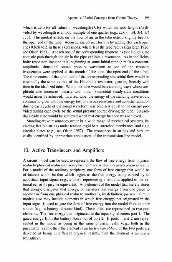
Imagine that, beginning at some initial time (t = 0) a constant-amplitude, sinusoidal sound pressure waveform at frequency Wr were applied (from a source of some sort) at the mouth of the tube (the end of the tube opposite the enclosed volume). The corresponding volume flow through the tube, into the enclosed volume, would approximate a ramp-modulated sine wave (e.g., tsinwt). Cycle by cycle, the amplitude of the sinusoidal volume flow of air through the tube would grow. Correspondingly, the amplitude of the sinusoidal pressure variations in the enclosed volume would grow. Those pressure variations would be precisely 180 degrees out of phase with the pressure variations at the source (at the other end of the tube). Thus the two pressure variations would reinforce one another in the creation of a net pressure difference from one end of the tube to the other. It is that net pressure difference that drives the flow through the tube. The growing flow through the tube and pressure in the enclosure represent a growing amount of acoustic energy stored in the resonant system. In the idealized example presented here, with no mechanism for dissipation of acoustic energy, it would continue to accumulate forever; sinusoidal steady state would never occur. In a real situation, at least two things will happen to the acoustic energy: (1) some fraction of it will be converted to heat by viscous resistance in the system, and (2) some fraction will be radiated from the mouth of the tube and the walls of the enclosure. When the total amount of acoustic energy gained from the source during each cycle is balanced precisely by the acoustic energy lost during each cycle, then sinusoidal steady state will have been achieved.
9.2 Standing-Wave Resonators In the Helmholtz resonator, one presumes that the wavelength of sound at the resonant frequency is very long in comparison to the dimensions of the enclosed volume and the tube. When that is not so, another form of resonance-a standing-wave resonance-can occur. Consider, for example, a rigid-walled tube filled with air. The acoustical driving-point impedance of the air in the tube, viewed from one end of the tube, is given by Equation 68. If the other end of the tube were sealed, making ZL exceedingly large, then the driving-point impedance would be approximated very well by the following expression:
ZdP = Zo----
i sin ( 2n~) (86)
Appendix: Useful Concepts from Circuit Theory 395
which is zero for all values of wavelength (A for which the tube length (L) divided by wavelength is an odd multiple of one quarter (e.g., U1., = 114, 3/4, 5/4 ... ). The inertial effects on the flow of air in the tube extend slightly beyond the open end of the tube. Acousticians correct for this by adding (for each open end) 0.82R to L in these expressions, where R is the tube radius (Rayleigh 1926; see Olson 1957). At each one of the corresponding frequencies (see Eq. 69), the acoustic path through the air in the pipe exhibits a resonance. As in the Helmholtz resonator, imagine that, beginning at some initial time (t = 0) a constantamplitude, sinusoidal sound pressure waveform at one of the resonant frequencies were applied at the mouth of the tube (the open end of the tube). The time course of the amplitude of the corresponding sinusoidal flow would be essentially the same as that of the Helmholtz resonator, growing linearly with time in the idealized tube. Within the tube would be a standing wave whose amplitude also increases linearly with time. Sinusoidal steady-state conditions would never be achieved. In a real tube, the energy of the standing wave would continue to grow until the energy lost to viscous resistance and acoustic radiation during each cycle of the sound waveform was precisely equal to the energy provided during each cycle by the sound pressure source driving the tube. Sinusoidal steady state would be achieved when that energy balance was achieved.
Standing-wave resonances occur in a wide range of mechanical systems, including flexible strings under tension, rigid bars, stretched membranes, and rigid circular plates (e.g., see Olson 1957). The resonances in strings and bars are easily identified by appropriate application of the transmission-line model.
10. Active Transducers and Amplifiers
A circuit model can be used to represent the flow of free energy from physical realm to physical realm and from place to place within any given physical realm. For a model of the auditory periphery, one form of free energy that would be of interest would be that which begins as the free energy being carried by an acoustical input signal (e.g., a tone), representing a stimulus applied to the external ear or its piscine equivalent. Any element of the model that merely stores that energy, dissipates that energy, or transfers that energy from one place to another or from one physical realm to another is, by definition, passive. Circuit models also may include elements in which free energy that originated in the input signal is used to gate the flow of free energy into the model from another source (e.g., a battery of some kind). These often are represented as two-port elements. The free energy that originated in the input signal enters port 1. The gated energy from the battery flows out of port 2. If ports 1 and 2 are represented in the model as being in the same physical realm (e.g., both in the pneumatic realm), then the element is an (active) amplifier. If the two ports are depicted as being in different physical realms, then the element is an active transducer.
396 E.R. Lewis
10.1 Passivity Implies Bidirectionality
The active nature of the two-port element is reflected in its parameters. Among other things, a passive, linear process must be reciprocal or antireciprocal. Lack of reciprocity or antireciprocity in a linear two-port element implies that the element is active. As a corollary of the Onsager reciprocity theorem, for example, one can state the following: if a transduction process (1) is not based on spinning elements (e.g., a spinning top or rotating charge), (2) operates linearly (e.g., over a small range about the origin), and (3) is not bidirectional, then it must be active. Linear, passive transduction processes based on spinning elements are antireciprocal (h12 = h21' Z12 = -Z21) (see Lewis 1996). To be passive, not only must a linear transduction process be bidirectional, it must be either reciprocal or antireciprocal (equally effective in both directions).
10.2 Gated Channels Are Active
On the other hand, gated channels are abundant in nervous systems. In circuit models, the elements representing gated channels would be active. The mechanical input to a stereovillar bundle in an inner-ear auditory sensor carries free energy that originated with the acoustical input to the external ear. This input modulates the opening and closing of the strain-gated channels, through which flows electric current driven by the endolymphatic voltage. The source of the free energy carried by the resulting electrical signal (hair cell receptor potential) is the endolymph battery, not the acoustical input to the ear. Acoustically derived energy modulates the flow of electrical energy from a battery-a quintessential active transduction process. In some instances the hair cell receptor potential, in turn, is applied to a transducer that produces force and motion in the stereovillar bundle (see Manley and Clack, Chapter 1, section 5.1). It is not clear, yet, whether this process is passive, involving merely the transfer of free energy from the receptor potential to the mechanical motion of the bundle, or active, involving the gating of energy from some other source, such as an adenosine triphosphate (ATP) battery, to the motion of the bundle.
10.3 Positive Feedback Can Undamp a Resonance for Sharper Tuning Whether or not the reverse transduction process (from receptor potential to stereovillar motion) is active, the forward transduction process (from stereovillar motion to receptor potential) definitely is. Thus there is a loop in which there is the possibility of power gain. It has been proposed that such gain could compensate, in part, for the power loss that must be imposed by the viscosity of the water surrounding the stereovillar bundle (see Manley and Clack, Chapter 1, section 5). Assuming that tuning of the hair cell is accomplished by mechanical resonance associated with the stereovillar bundle, for example, one can depict the essential ingredients of this proposition with the circuit model of
Appendix: Useful Concepts from Circuit Theory 397
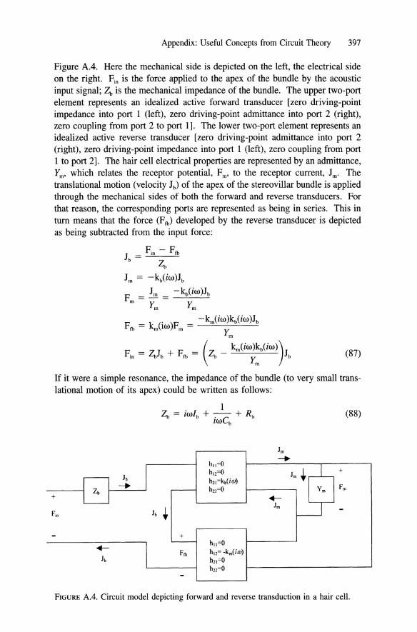
Figure A,4. Here the mechanical side is depicted on the left, the electrical side on the right. Fin is the force applied to the apex of the bundle by the acoustic input signal; ~ is the mechanical impedance of the bundle. The upper two-port element represents an idealized active forward transducer [zero driving-point impedance into port 1 (left), zero driving-point admittance into port 2 (right), zero coupling from port 2 to port 1]. The lower two-port element represents an idealized active reverse transducer [zero driving-point admittance into port 2 (right), zero driving-point impedance into port 1 (left), zero coupling from port 1 to port 2]. The hair cell electrical properties are represented by an admittance, Ym, which relates the receptor potential, Fm, to the receptor current, Jm. The translational motion (velocity Jb) of the apex of the stereovillar bundle is applied through the mechanical sides of both the forward and reverse transducers. For that reason, the corresponding ports are represented as being in series. This in turn means that the force (Fib) developed by the reverse transducer is depicted as being subtracted from the input force:
J = Fin - Fib b ~
Jm = -lG,(iw)Jb Jm -kb(iw)Jb
F=-=-.e..:....-~ m Ym Ym
Fib = ~(iw)Fm = -~(iW~lG,(iW)Jb m
F = ~J + F = (~ _ ~(iW)lG,(iW))J In b Ib Ym b (87)
If it were a simple resonance, the impedance of the bundle (to very small translational motion of its apex) could be written as follows:
+
Fin Jb
.-Jb
1 ~ = iw1b + -. - + Rb
zwCb
hll;O h'2;O h2,;kb(iw) h22;O
• +
hll=O
Fib h'2; -km(iw) h2,;Q h22;O
(88)
J,.
-+ +
Fm
.-Jm
FIGURE A.4. Circuit model depicting forward and reverse transduction in a hair cell.

398 E.R. Lewis
where Ib is the inertance of the bundle, Cb is its elastic compliance, and Rb is the resistance of the bundle (owing at least in part to the viscosity of water). With the transducers in place, the relationship between bundle motion (velocity) and input force becomes
(89)
The net resistance, which damps the resonance, is equal to
(90)
To be effective for undamping the resonance, the quantity Re{ ~~ } should be
greater than zero and less than Rb• If it is greater than Rb , the resonance will oscillate spontaneously. If it remains in the proper range, the pair of active transducers will operate as a stable amplifier (Manley and Clack, Chapter 1, section 5). The effect of this on tuning is depicted in Figure A.5, which shows the phase and amplitude tuning curves of a damped resonance. The bottom panel in Figure A.S shows the temporal response (e.g., velocity) of the resonance as its residual energy decays after the input has ceased. Notice that as the resonance becomes less damped, its tuning peak becomes sharper but it requires more time to rid itself of residual energy. The latter reflects both the advantage and the disadvantage of resonance tuning. It allows the response to an ongoing input signal to accumulate over time. In a quiet world, where the threshold of hearing is limited by the internal noise of the ear, this should enhance the ability of the hearer to detect the presence of the signal. At the same time, it would reduce the temporal resolution with which the hearer could follow amplitude changes in the signal, once the signal has been detected.

Appendix: Useful Concepts from Circuit Theory 399
- 10 en "'C - 0 Q) "'C :I
~-10
~ -20
0.05 0.1 0.2 0.3
5 Frequency (kHz)
-"'C e -Q) 0 (/)
«I ~ a.
-5 0.05 0.1 0.2 0.3
Frequency (kHz)
1
0.5
0
-0.5
-1 0 100 200 300
Time (ms)
FIGURE A.S . Tuning of a IOO-Hz resonance with a high degree of damping (solid black line) and a reduced degree of damping (thick gray line). The bottom panel shows the time course of decay for residual excitation in the resonance.
400 E.R. Lewis
References Baranek LL (1954) Acoustics. New York: McGraw-Hill. Ewing AW (1989) Arthropod Bioacoustics. Ithaca, NY: Cornell University Press. Lewis ER (1984) Inertial motion sensors. In: Bolis L, Keynes RD, Maddrell SHP (eds)
Comparative Physiology of Sensory Systems. Cambridge: Cambridge University Press, pp. 587--610.
Lewis ER (1996) A brief introduction to network theory. In: Berger SA, Goldsmith W, Lewis ER (eds) Introduction to Bioengineering. Oxford: Oxford University Press, pp.261-338.
Lewis ER, Narins PM (1998) The acoustic periphery of amphibians: anatomy and physiology. In: Fay RR, Popper AN (eds) Comparative Hearing: Fish and Amphibians. New York: Springer-Verlag, pp. 101-154.
Morse PM (1981) Vibration and Sound. New York: Acoustical Society of America. Olson HF (1957) Acoustical Engineering. Princeton, NJ: D. van Nostrand. Olson HF (1967) Music, Physics and Engineering. New York: Dover. Onsager L (1931) Reciprocal relations in irreversible processes: I, II. Phys Rev 37:405-
426; 38:2265-2279. Rayleigh (1926) Theory of Sound. London: Arnold. Talbot L (1996) Fundamentals of fluid mechanics. In: Berger SA, Goldsmith W, Lewis
ER (eds) Introduction to Bioengineering. Oxford: Oxford University Press, pp. 101-132.

Index
Absorption, sound in air, 36-37 Acanthostega, evolution, 165
inner ear, 133-134 skull, 131, l32-l33
Acetylcholine, hair cell efferent neuro-transmitter, 59
Acoustic physics, 369ff Acoustic scene, hearing evolution, 100 Acoustic wave equation, derivation, 372ff Acoustic waves, properties, 41 ff Acoustics, resonance, 393-395
review, 369ff Actinopterygia (ray-finned fishes), 6 Active amplification, hair cell, 18-19,
364-365 Active process, lizards, 18-19,207
reptiles, 69 reptiles and amphibians, 211
Afferent terminal number, birds, 246ff Afferents, S 1 and S2 in saccular nerve,
62 African clawed frog, see Xenopus laevis Agamid lizards, hair cell types, 69 Agnatha, evolution of ear structures,
100ff earliest ears, 97 inner ear, 75-76
Allosaurus fragi/is, vestibular apparatus, 234ff
Alosa sapidissima (American shad), ultrasonic hearing, 117
Ambystoma tigrinum (tiger salamander), amphibian papilla, 185
torus semicircularis, 322 American shad, see Alosa sapidissima Amia calva (bowfin), labyrinth, 106-107
Amniote, basilar papilla origin, 8ff evolution of stapes, 139, 140ff hair cell tuning, 15ff hearing principles, 15ff inner ear, 8 middle ear evolution, l37ff phylogeny, 10 skull evolution, 137ff
Amos gene, mechanoreceptors, 84 Amphibian papilla, 7-8, 66, 169ff
Ambystoma tigrinum, 186 electrical tuning of hair cells, 187, 188 epithelia structure, 185ff hair cell orientation patterns, 188-189 pressure reception, 182ff relationship to macula neglecta, 183-
184 tadpole, 177
Amphibians, saccule, 169 amphibian papilla, 7-8, 66, 169ff, 187-
189 auditory brainstem, 300 auditory midbrain organization, 327 basilar papilla, 7-8, 172-173 development of inner ear, 189-190 diversity of ear structure, 168ff ear anatomy, 166ff ear evolution, 135-137, 164ff evolution of middle ear, 173ff hair cells, 64ff hearing, 166-168 impedance match, 173 middle ear, 173ff origin and evolution, 2-4, 165-166 origin of basilar papilla, 184-185 papilla neglecta, 169-170, 183-184
401

402 Index
Amphibians, saccule (continued) periotic canal and hearing, 179-181 saccule and seismic detection, 178, 181-
182 sound pathways, 166-168 stapes, 166-168, 173 time pattern discrimination, 331 tympanic ear, 135-137, 173 underwater hearing, 164 see also Frog, Salamander, Tadpole
Amphioxus (lancelet), hearing, 97 Amphisbaenids, basilar papilla, 214 Amplitude modulation, lTD processing,
319-320 rate representation in midbrain, 331
Anabantids, hearing mechanisms, 110, 113
sound production, 116 Analogy, defined, 290 Anas platyrhynchos (mallard duck), audi
ogram, 232-233 hair cells, 71
Ankle links, hair cells, 59 Anterior forebrain pathway, birdsong, 342 Anterior octaval nucleus, fish hearing,
299-300 Antrozous fuscus, duration coding in mid
brain, 333 Antrozous pallidus (pallid bat), duration
coding in midbrain, 333 Anurans, see Amphibians Archaeopteryx (primitive bird), otic re
gion, 143 archosaur evolution, 226
Archistriatum, and arcopallium in birds, 337
Archistriatum, birdsong, 329, 342-343 Archosaur, basilar papilla compared to
primitive mammals, 249-250 hair cells, 11-13, 69ff hearing organ evolution and specializa
tion, 13-14, 224ff nucleus magnocellularis, 301
Archosauromorphs, middle ear, 142-143 Arcopallium, and archistriatum in birds,
337 Arius felis (marine catfish), labyrinth, 108
low-frequency hearing, 108 Ascaphus truei, hair cells, 64-65
Astronotus ocellatus (oscar), gentamycin effects, 62
hair cells, 61-62 lagena and gentamycin, 62
Atonal gene, 290 Atonal transcription factor, hair cells, 83-
84 Audiograms, various fish species, 112ff Auditory CNS, basic vertebrate plan, 297
evolution, 289ff see also CNS
Auditory forebrain, 335ff common features, 336ff, 345 dorsal and ventral pallium, 335ff primates, 339-340 "what" and "where" functions, 339-
340 Auditory midbrain, 298
common features of processing, 335 core and belt organization, 326-327 descending connections, 329 fishes and amphibians, 323ff inputs, 327-328 and motor systems, 328-329 nucleus centralis, 323ff projections to forebrain, 337 response property transformations, 328 temporal processing, 329ff various species, 325
Auditory space, population codes in forebrain, 340
Aves, see Birds Aythya fuligula (tufted duck), basilar pa
pilla dimensions, 237-238
Bandwidth of hearing, early mammals, 279-281
evolution in fishes, 99 Bam owl, see Tyto alba Basilar membrane, high-frequency hear
ing, 272 Basilar papilla, amphibian, 7-8, 66, 172-
173 archosaurs, 69ff evolution, 8ff, 184-185, 294 evolution in reptiles, 213ff evolution of elongation, 19-20 Gekko, 207 hair cell orientation patterns, 188-189
hair cell resonances, 187-188 homology between amphibian and am-
niote structures, 184-185 innervation in amphibians, 185 Latimeria, 7 lizards, 200ff mechanics, 211 pressure reception, 182ff relationship to lagena, 184-185 reptiles, 11 ff, 66ff sauropsids, 300 stereovilli height in birds, 239-240 subpapillae in lizards, 220 tadpole, 177 turtle, 10-11
Basilar papilla frequency map, various bird species, 228ff
Basilar papilla innervation, implications in birds, 249ff
Basilar papilla length, frequency range of hearing in birds, 232-233
Basilar papilla width, various bird species, 238ff
Bats, cortical mechanisms, 344-345 IC frequency maps, 327
bHLH gene, auditory CNS, 295 Bidirectional-type hair cells, hair cell
groups in reptiles, 69, 209ff Binaural cues, processing in birds and
mammals, 310ff Binaural processing, auditory forebrain,
339-340 delay lines, 313
Biologically significant sounds, forebrain pathways, 338
Birchir, see Polypterus Bird, ear, 11ff
cochlear amplification, 271 cochlear nuclei, 304ff hair cell innervation and specialization,
21,23 hair cells, 69ff hearing organ evolution and specializa-
tion, 224ff middle ear in early species, 143 nucleus angularis, 301 relationship to dinosaurs, 6, 235 stereovilli height, 239-240
Bird basilar papilla, widths, 238ff
Index 403
Bird body size, basilar papilla length, 234ff
Bird body weight, hair cell number, 236-237
Bird common ancestor, basilar papilla features, 237
Birdsong, and human speech, 340ff BK channels, turtle hair cells, 67 Bloch's catfish, see Pimelodus blochi Bobtail skink, see Tiliqua regosa Bony fish, see Osteichthyes Borylloides violaceus (sea squirt), coronal
organ, 78-79 Botryllus schlosseri (sea squirt), coronal
organ, 78-79 Bowfin, see Amia calva Brachiosaurus brancai (sauropod dino
saur), inner ear, 234ff Brainstem, special adaptations, 299ff Branchiostoma fioridae (lancelet), hair
cells, 76 Brass instruments, sound sources, 34-35 Brevoortia patronis (menhaden), ultra
sonic hearing, 117 Brienomyrus niger, lacking sound produc
tion, 116 Broca's area, speech, 341-342 Brown bullhead catfish, see lctalurus
nebulosus Budgerigar, see Melopsittacus undulatus Bullfrog, see Rana catesbeiana Bullhead catfish, see Ictalurus nebulosus Bushy cells, lTD processing, 310
Caecilians, hair cells, 64 Caenorhabditis elegans, mechanoreceptor
channel, 80-81 Caiman crocodilus (caiman), basilar pa
pilla, 248 frequency map, 228ff hearing organ evolution and specializa
tion, 224ff papillar length and body size, 236-237 tall and short hair cells, 241
Calcium binding protein (S-lOO), hair cells, 61
Calcium/calmodulin kinase II, outer hair cells, 73
Calyx, Type I hair cells, 60

404 Index
Calyx of Held, MNTB, 317 Calyx terminals, birds, 306 Carassius auratus (goldfish), audiogram,
112 saccular hair cells, 62, 63 sound discrimination, 99 Weberian ossicles, 111
Catfish, see also lctalurus sp., Silurus sp. hearing specializations, 109 labyrinth, 107-108 sound production, 116
Cave swiftiet, see Collocalia linch Central auditory pathways, evolution,
289ff see also CNS
Central auditory system, see CNS Cephalochordates, hair cells, 75ff
inner ear, 76-77 Cephalopods, ciliated mechanoreceptors,
79 Ceratodus forsteri, labyrinth, 106-107 Channel catfish, see letalurus punctatus Characids, sound production, 116 Chelonia, see Turtles Chicken, see Gallus gallus domesticus Chiclids, hearing mechanisms, 110 Chimaera monstrosa (ratfish), lateral line
hair cells, 63 labyrinth, 103
Chondrichthyes, labyrinth, 102ff Chopper cells, in various taxa, 308 Chordates, non-vertebrate hair cells, 75ff Chordotonal organs, Drosophila, 80 Cilial motility, Drosophila, 80 Circuit theory metamodel, 30-31, 369ff
physics of sound, 369ff Cladistic analysis, 1-2 Cladogram, fish hearing organs, 96
lizard families, 212 vertebrate, 3
Clupeids, ultrasonic hearing, 117 CNS, basic design, 296ff
evolution, 289ff evolution of lateral line system, 292-
293 origins, 289ff
Cochlea, and lagena, 278-279 coiling, 275, 278-279 comparative anatomy, 265ff
extinct mammals, 272ff function, 263-265 marsupials, 265-267 Mesozoic mammals and monotremes,
267ff, 273ff Alorganucodon, 154 therian mammals, 275-278 tuning, 263-265 see also Inner ear
Cochlear amplifier, birds and reptiles, 271 evolution, 263-265, 270-272 monotremes, 270-271 otoacoustic emissions, 271-272
Cochlear function, Alonodelphis, 264 monotremes and marsupials, 264
Cochlear nucleus, and airborne sound, 304
mammalian cell types, 306ff parallel evolution of cell types, 304 special adaptations, 299ff species diversity, 297-298 subdivisions, 301-302 terrestrial vertebrates, 298
Cod, see Gadus morhua Coelacanth, fossil ears, 130-132
see also Latimeria chalumnae Collocalia linch (cave swiftlet), vocaliza
tion, 224-225 Columba livia (pigeon), hair cells, 71
infrasound, 225-226 Columbiformes, evolution, 227 Columella, origin in early tetrapods, 133 Combination-sensitive neurons, bat CNS,
333ff Communication, archosaurs, 224ff
in fishes, 115-116 later evolution of, 98
Communication sounds, early evolution, 98
forebrain processing, 335, 337 HV c response in birds, 338 midbrain processing, 331-332 transmission effects in fishes, 99
Cortex, and dorsal pallium, 338 Cortical maps, bats, 344-345 Corydoras paleatus (lumpsucker), hearing
ability, 113 Craniates, hair cells, 75ff Croaking gourami, see Trichopsis sp.
Crocodilia, ear, 11ff hair cells, 69ff hearing organ evolution and specializa
tion, 224ff middle ear, 143
Cross-correlation, nucleus 1arninaris, 311ff
Crossopterygia, 2 C-start, fishes, 117 Cuticular plate, archosaurs, 71 Cyclopterus lumpus (lump fish), labyrinth,
107 Cyprinids, sound communication, 116
Damselfish, see Eupomacentrus Delay lines, and auditory midbrain, 327-
328 binaural circuits, 313
Delay tuning, bat midbrain, 333-334 Descending auditory system, 299 Descending octaval nucleus, fish hearing,
299-300 Diapsids, ear, llff Didelphis virginiana (Virginia opossum),
hearing range, 262 Dinosaurs, see also Brachiosaurus sp.
middle ear, 142-143 relationship to birds, 6
Distalless gene, 290 Distortion Product Otoacoustic Emission,
see DPOAE DNA hybridization, evolution of birds,
227-228 Doppler shift, 42-43 Dorsal ventricular ridge (DVR), auditory
forebrain, 337-338 Dorsolateral nucleus (DLN), anurans,
300ff DPOAE, marsupial, 264-265
Monodelphis, 264-265 Dromaius novaehollandiae (emu), audi
tory nerve frequency response, 228 basilar papilla dimensions, 237-238 hair cells, 70-71
Drosophila (fruit fly), ciliated mechanoreceptors, 75, 79ff
Duck-billed platypus, see Onnithorhynchus anatinus
Duration encoding, midbrain, 331, 333
Index 405
Ear, Acanthostega, 132-133 amphibian structure and diversity, 166ff approaches to study of evolution, 360 bird, lIff crocodilian, 11 ff diapsids, 11ff early tetrapods, 132ff evolution in amphibians, 135-137 lissamphibians, 135-137 mammals, 15, 256ff salamander, 137,174 shape in different mammalian taxa, 258 snakes and lizards, 13-14 synapsids, 15 tadpole, 177-178 Ternnospondyls, 135-137 Xenopus laevis, 173-174
Ear evolution, and other sensory path-ways, 292ff
Ear structure, evolution in fishes, 100ff Eavesdropping, early hearing function, 98 Echnidna, see Tachyglossus aculeatus Echolocation, midbrain processing, 333ff Efferent innervation, bird basilar papilla,
245ff Carassius saccular hair cells, 62
Efferent synapses, archosaurs, 69 hair cells, 59--60
Efferents, evolution, 291-292 outer hair cell motility, 73
Elasmobranchs (cartilaginous fish), vestibular hair cells, 63
Electrical tuning, amphibian papilla hair cells, 187, 188
amphibian saccular hair cells, 187, 188 hair cell, 16-17,46 turtle hair cells, 203ff
Electromotility, outer hair cells, 73 Electroreception, relation to CNS evolu
tion, 293 Elephant-nose fish, see Gnathonemus
petersii Eleutherodactylus coqui (coqui frog),
sound duration processing, 331 Emu, see Dromaius novaehollandiae Entosphenus japonicus (Japanese lam
prey), hair cells, 63 Environment, combined effects on sound,
35ff,39-41

406 Index
Eptesicus fuscus (little brown bat), duration coding in midbrain, 333
Eptesicus fuscus, Ie frequency map, 327 Eupomacentrus dorsopunicans (dusky
damselfish), audiogram, 112 Eupomacentrus partitus (bicolor damsel
fish), hearing ability, 109 sound production, 116
Eurasian ruffe, see Gymnocephalus cemuus
European catfish, see Silurus glanis Eusthenopteron, skull, 131, 132-133 Eutherians, see Mammals Evolution, Acanthostega, 165
active amplification by hair cells, 364-365
amniote middle ear, 137ff amphibian ear, 164ff amphibian middle ear, 173ff, 176 amphibian papilla, 169ff amphibians, 165-166 auditory eNS, 368 basilar papilla, 19-20 cochlear amplifier, 270-272 columella, 133 ear in fishes, 365-366 ear in tetrapods, 365-366 ear ontogeny, 189-190 hair cell, 6-8 hair cell specializations, 20-21 hair cell tuning, 15ff hair cells of different types, 366 high-frequency hearing, 17-18 impedance matching, 365-366 lizard ear, 14 mammals, 257ff mechanoreceptor cells, 361-363 middle ear, 128ff, 145ff middle ear in archosauromorphs, 142-
143 middle ear in neodiapsids, 140ff middle ear in spenodontids, 141 middle ear in synapsids, 145ff optimization of free energy transfer in
ear, 389-390 pressure receiver, 176ff selective pressures on hearing, 27ff sense of hearing, 362 stapes, 133-135, 137
stream segregation, 28-29 tetrapod hearing, 128ff therapsid middle ear, 148-149 tympanic ear, 146ff, 366
Extinct mammals, cochlea, 272ff Extinct monotremes, cochlea, 273-275
Far field, 98 Fence lizard, see Sceloporus occidentalis Fibroblast growth factor (FGF), 290 Field L, bird forebrain, 337, 343
sharp tuning, 338 Fire salamander, see Salamandra
salamandra Fish, definition of term, 2
ears and auditory eNS, 299-300 evolution of ear, 6, 365-366 hearing organs and parallel evolution,
95ff hearing sensitivity, 176, 363 inner ear hair celis, 61 ff temporal processing in midbrain, 330
Forebrain, see also Auditory forebrain uniqueness among mammals, 343ff
Fossil ears, coelacanth, 130-132 Fossils, early tetrapods, 132ff Frequency map in birds, compression at
low frequencies, 229ff slope, 231-232
Frequency range of hearing, bird basilar papilla, 232ff
Frog, see also Amphibians auditory forebrain, 337 ear, 137 interaural cues, 310 sound production mechanisms, 136
Fundus, basilar papilla in geckos, 211
GABA, and MSO inhibition, 316 hair cell efferent neurotransmitter, 59 lateral lemniscus, 320-321 NA and NL inputs in birds, 313ff
Gadus morhua (Atlantic cod), audiogram, 112
hearing abilities, 109ff ultrasonic hearing, 117
Galliformes, evolution, 227 Gallus gallus domesticus (chicken), hair
cell currents and channels, 71
hair cells, 71 inner ear, 224-225 nucleus laminaris, 312
Gastrulation homeobox gene (gbx), 290-291
GATA3 gene, auditory nerve, 295 Gecko, see Gekko gecko Gekko gecko (Tokay gecko), basilar pa
pilla, 210-211 basilar papilla tonotopy, 207 hair cell innervation, 216ff
Geological time scale, 5 Gerrhonotus multicarinatus (alligator liz
ard), frequency selectivity, 218ff Globular bushy cells, in various taxa, 309 Glutamate, hair cell neurotransmitter, 59-
60 Glycine, and MSO inhibition, 316--317
hair cells, 60 Gnathonemus petersii (elephant-nose
fish), audiogram, 112 Goldfish, see Carassius auratus Gonorhynchiforms (milkfish), relationship
to Otophysi, 128 Granite spiny lizard, see Sceloporous
orcutti Grass frog, see Rana esculenta Guinea fowl, see Numida meliagris Gymnocephalus cernuus (Eurasian ruffe),
audiogram, 112 Gyrnnophiona, middle ear, 174-175
Habitat, hearing mechanisms in fishes, 114-115
Hagfish, inner ear, 75-76 see also Myxine glutinosa
Hair cell, 55ff active amplification, 18-19 archosaur, 11-13 basilar papilla, 187-188 channels and currents, 203ff currents in goldfish saccule, 62-63 electrical resonance, 16--17, 46 electrical tuning in amphibian papilla,
187, 188 evolution, 6--8, 55ff, 81ff, 361-363 evolution of active amplification, 364-
365 evolution of different types, 366
Index 407
functional gradient, 21-23 general morphology, 56ff and invertebrate ciliated mechanorecep-
tors, 81ff lateral line, 7 mammalian cochleae, 265-267 marsupial cochlea, 265-267 Mathl gene, 290-291 mechanical tuning, 17-18 monotreme cochlea, 267ff number of stereovilli in birds, 239-240 and phylogeny, 56ff specialization of function, 20-21 spikes in Carassius saccule, 62 tuning, 15ff tuning mechanisms in reptiles, 204-
205 types, 7
Hair cell conductances, amphibians, 65 Hair cell development, genes, 270 Hair cell dimensions, basilar papilla of
birds, 241ff, 245ff Hair cell innervation, birds, 23
lizard basilar papilla, 217 mammals, 22
Hair cell motility, monotremes, 271 Hair cell number, papillar length in birds,
234ff Hair cell orientation patterns, amphibian
papilla, 188-189 basilar papilla, 188-189 lizards, 67ff
Hair cell specializations, reptiles, 206--207
Hair cell tuning, evolution, 15ff temperature dependence, 205
Hair cell types, innervation patterns in birds, 244ff
Hearing specializations, amphibians, 166-168
definition, 31 Didelphis virginiana, 262 early mammals, 279-281 evolution, 27ff fishes, 99, 108ff, 176 high frequency in mammals, 279-281 high-frequency specializations, 272 increasing sensitivity, 363-364 Morganucodon, 154, 279-280

408 Index
Hearing specializations, amphibians (continued)
origins, 362 osteolepiforms, 132 range in mammals, 260ff range in marsupials, 261, 262 range in Monodelphis, 261, 262 range in monotremes, 261, 262-263 range in Omithorhynchus anatinus,
262-263 role of periotic canal in amphibians,
179-181 salamander, 174 tadpoles, 177-178 tetrapod ancestors, 130 underwater by Xenopus, 174
Herrings, ultrasonic hearing, 117 Hesl gene, hair cell development, 270 Higher vocal center (HVc), bird fore-
brain, 338, 342 High-frequency hearing, advantages, 279-
281 specializations, 272
Homology, defined, 290 lacking between NL and MSO, 318
Horseshoe bat, see Rhinolophus rouxi Human beings, stream segregation, 29, 50-
51 Hyomandibular, conversion to columella,
133 Hypothalamus, and auditory pathway, 336
IC, see Inferior colliculus, Auditory midbrain
Ictalurus nebulosus (brown bullhead catfish), hearing sensitivity, 112
Ictalurus punctatus (channel catfish), hearing ability, 113
Impedance, driving point, 387ff terminal, 385-387
Impedance matching, amphibians, 173 auditory system, 48-49 coming on to land, 364 evolution, 365-366 fish ears, 96
Impedance mismatch, 173 Implosions, as sound source, 32 Inferior colliculus, see also Auditory
midbrain evolution and homology, 322ff
llD processing, 320-321 various species, 325
Infrasound, fish behaviors, 118 Infrasound detection, archosaurs, 225-
226,233-234 Inner ear, see also Cochlea, Ear
Acanthostega, 133-134 amniote, 8 development in amphibians, 189-190 early tetrapods, 133-134
Inner hair cells, 72ff marsupials, 265-267 monotremes, 267ff
Interaural cues, processing in various taxa,31Off
Interaural intensity differences, processing in birds and mammals, 320ff
Interaural level differences (lID), 310ff Interaural time differences (lTD), 310ff
avian vs. mammalian processing, 317 Interaural time processing, archosaurs,
311ff Interaural time processing, circuits in
mammals and birds, 313ff Isocortex, origins, 338
Japanese lamprey, see Entosphenus japonicus
lawless fishes, hair cells, 63-64 Jeffress, space map, 313 Johnston's organ, Drosophila, 80
Kinocilium, 58 Kinocilium bulbs, amphibians, 65
Lagena, dinosaur fossils, 234ff hearing in fishes, 108 origins of cochlea, 278-279 relationship to basilar papilla, 184-
185 Lambdopsalis bulla (a multituberculate
mammal), inner ear, 274 Laminar nucleus, torus semicircularis,
326 Lampetra fluviatilis (river lamprey), hair
cells, 55, 61, 63-64 labyrinth, 10 1-102
Lamprey, 63 see also Branchiostoma floridae, En
tosphenus, Lampetra, Petromyzon

Lateral lemniscus, lID processing, 320-321
species diversity, 297-298 Lateral line neuromasts, gentamycin, 63 Lateral line system, 55
hair cells, 7, 61ff Lateral superior olive, lID processing,
321ff Latimeria chalumnae (coe1acanth), basilar
papilla, 7 ear, 7 hearing, 130 phylogeny, 2
Learning, birdsong and human speech, 340ff
Leopard frog, see Rana pipiens Lepidosaurs, lizard evolution, 201-202 Lissamphibia, see also Amphibians
ear, 135-137 Little brown bat, see Eptesicus fuscus Lizards, afferent and efferent synapses, 69
ear, 13-14 evolution of basilar papilla, 14, 67ff,
200ff, 214ff hair cells, 67ff nucleus magnocellularis, 301 papillar lengths, 217-218
Lobe-fins, see Sarcopyterygia Low-frequency hearing, importance for
birds, 250 Lumpfish. see Cyclopterus lumpus Lumpsucker, see Corydoras sp. Lungfish, hearing, 130
see also Ceratodus forsteri
Macromechanics, lizard basilar papilla. 211
Macropodus opercularis (paradise fish), hearing mechanisms. 113-114
Macula communis, Myxine, 101-102 Macula neglecta, amphibians, 183-184
relationship to amphibian papilla, 183-184
sharks, 104 see also Papilla neglecta
Mallard duck, see Anas platyrhynchos Mammals, cochlea in extinct species, 272ff
cochlear function, 263-265 ear, 15, 256ff ear shape in different taxa, 258
evolution, 257ff fossil record, 259-260 hair cell innervation, 22
Index 409
hair cell specialization, 21, 22 hair cells, 72ff hearing in early species, 259, 279-281 hearing range, 260ff middle ear evolution, 153ff systematics and phylogeny, 257ff unique forebrain mechanisms, 343ff
Mandible, see Middle ear Marine catfish, see Arius felis Marmoset, twitter calls and cortex, 344 Marsupials, cochlear anatomy, 265-267
cochlear function, 264 DPOAE,264-265 hearing range, 261 systematics, 257, 259
Masking, fishes, 100 MathI gene, 290, 295
hair cell development, 270 Mauthner cell, 117, 296 Mechanical tuning, hair cell, 17-18 Mechanoreceptor cells, evolution, 361-
363 Mechanotransduction, defined, 59 Medial geniculate complex, mammals,
299, 338 Medial olivary efferent system, 73 Medial superior olive, and frequency
range of hearing, 318-319 evolution, 317ff interaural time processing, 315ff and nucleus laminaris, 315ff space map, 317
Melopsittacus undulatus (parakeet), critical masking ratio, 225-226
Mesozoic mammals, cochlea, 273ff Mesozoic therian mammals, inner ear,
275-278 Micromechanical tuning, reptiles, 204ff,
207 Midbrain, evolution and homology, 322ff
see also Auditory brainstem, Brainstem, Inferior colliculus, Torus semicircularis
Middle ear binaural coupling, 310-311 amphibians, 173ff archosauromorphs, 142-143 crocodilians, 143
410 Index
Middle ear binaural coupling (continued) dinosaur, 142-143 early turtle, 143-145 evolution, 128ff evolution in amniotes, 137ff evolution in amphibians, 176 evolution in mammals, 155-157 evolution in neodiapsids, 140ff evolution in pelycosaurs, 151 evolution in stem mammals, 153-155 evolution in therapsids, 152 evolution in theriodonts, 152-153 evolution of three ossicles, 146ff frequency range of hearing in birds,
233 Gymnophiona, 174-175 lizards, 201 monotreme, 155, 156 Morganucodon, 150, 153-154 periotic canal in amphibians, 179-181 pressure reception, 178-179 salamander, 174 sound production in Rana catesbeiana,
174-175 spenodontids evolution, 141 squamate evolution, 141-142 synapsids, 145ff theories of evolution, 145ff turtle, 10
Midshipman fish, see Porichthys notatus Monodelphis domestica (short-tailed
opossum), cochlear function, 264 cochlea in Mesozoic species, 273-275 cochlear amplifier, 270-271 cochlear anatomy, 267ff cochlear function, 264 hair cells, 72 hearing range, 261, 262 middle ear, 155, 156 outer hair cells, 271 pillar cells, 269-270 stereo villi, 272 systematics, 257, 259
Morganucodon (primitive mammal), bin-aural processing, 319
cochlea, 154, 250 hearing capabilities, 154, 279-280 inner ear, 273 middle ear, 150, 153-154
Mormyrids, hearing mechanisms, 113, 115
Motility, outer hair cells, 73 stereo villi, 69
Motor systems, and auditory midbrain, 328-329
Multituberculates, cochlea, 272-273 Musical instruments, as sound sources, 34-
35 Mustached bat, see Pteronotus parneliii Myripristus kuntee (squirrelfish), audi
ogram, 112, 114 hearing mechanisms, 110
Myxine glutinosa (hagfish), evolution of ear structures, 100-10 1
hair cells, 55 inner ear, 75-76, 101-102
Myxiniformes (hagfishes), inner ear, 75-76
Myxiniformes, lateral line system, 76
Nautilus, ciliated mechanoreceptors, 79 Near field, sound detection evolution, 98 Neodiapsids, middle ear evolution, 140ff Neurogenin, auditory CNS, 295 Neutral evolution, lizard basilar papilla,
200ff NMDA receptors, Type I hair cells, 60 NompC, Drosophila mechanosensory
channel, 80-81 Norhern tegu lizard, see Tupinambis
nigropuncatus Notch pathway, 84 Nucleus angularis, 301
chopper cells, 308 lID processing, 320-321 sauropsids, 300 type IV response type, 306
Nucleus centralis, auditory midbrain, 323ff
Nucleus laminaris, and superior olive, 311ff
archosaurs, 298 evolution, 317ff
Nucleus magnocellularis, sauropsids, 300
Nucleus mesencephalicus lateralis pars dorsalis (MLD), auditory midbrain, 322ff

Numida meliagris (Guinea fowl), midbrain vocalization processing, 332-333
Octaval nerve, 296 Octopus cells, in various taxa, 309 Octopus vulgaris, ciliated mechanorecep-
tors, 79 Oil bird, see Steatomis caripensus Onset responses, in various taxa, 308-309 Ontogeny, evolution of ear, 189-190 Opossum, see Didelphis, Monodelphis Opsanus beta (toadfish), torus semicircu-
laris, 324 Opsanus tau (oyster toadfish), audiogram,
112 hair cell physiology, 62-63
Organ of Corti, see Cochlea Omithorhynchus anatinus (duck-billed
platypus), hearing range, 262-263 Orthodenticle (otx) transcription factor,
290-291 Oscar, see Astronotus ocellatus Ostariophysi, 6
evolution of Weberian apparatus, 128, 130
hearing mechanisms, 114-115 labyrinth, 107-108 relationship to Otophysi, 128
Osteichthyes, cladistics, 2 labyrinth, 104ff
Osteolepiforms, hearing, 132 Ostracoderms, vestibular labyrinth, 97 Otoacoustic emissions, cochlear amplifier,
20-21, 271-272 reptiles, 211 see also DPOAE
Otolith organs, fishes, 61 ff Otoliths, and otoconia, 105-106
coelacanth, 130 fish hearing, l04ff
Otophysi, relationships in Ostariophysi, 128
Outer hair cells, 72ff currents and channels, 73 marsupials, 265-267 monotremes, 267ff, 271 tuning, 263-265
Index 411
Paleozoic, tetrapod ears, 132ff Papilla neglecta, amphibians, 169-170
see also Macula neglecta Paradise fish, see Macropodus opercularis Parakeet, see Melopsittacus undulatus Parallel evolution, fish hearing organs,
95ff Parallel evolution, sound source localiza-
tion circuits, 309ff Parareptiles, see Turtles Pars inferior, labyrinth, 170 Pars superior, labyrinth, 169-170 Particle displacements, 380-382 Particle velocity, 380 Passeriformes, evolution, 227 Pax6 gene, 290 Pelycosaurs (basal synapsids), middle ear
evolution, 151 Periotic canal, comparative, 179-181 Periotic space, fish and amphibians, 176 Petromyzon jiuviatilis (river lamprey), lab-
yrinth, 101-102 Petromyzon marinus (sea lamprey), hair
cells, 63 Phylogeny, amniotes, 10
lizards, 201-202 mammals, 257ff vertebrate, Iff
Physics of sound, 369ff Pigeon, see Columba Livia Pike perch, see Stizostedion lucioperca Pillar cells, monotremes, 269-270 Pimelodus blochi (Bloch's catfish), mus-
cles on Weberian ossicles, 119 Pimelodus pictus, hearing ability, 113 Platydoras costatus (striped Rahael cat
fish), audiogram, 112-113 Platypus, see Omithorhynchus anatinus Podarcis (European wall lizard), tonotopy,
208 Pollimyrus adspersus (weakly electric
fish), torus semicircularis, 323-324 Pollimyrus isidori, sound production, 116 Polypterus (bichir), labyrinth, 106-107 Polypterus, sound production, 98 Population codes, auditory space, 340 Porichthys notatus (midshipman), vocal
signal processing, 330-331 torus semicircularis, 324
412 Index
Posterior forebrain pathway, vocal production, 342
Potassium currents, voltage-activated, 60
Pressure detection by tetrapods, evolution, 176ff, 294ff
Pressure receiver, middle ear, 178-179 Pressure-gradient receiver, anuran ears,
310 Prestin, hair cell motility, 73 Primary-like cells, in various taxa, 309 Primitive mammal cochlea, compared to
archosaurs, 249-250 Pseudemys scripta elegans (red-eared
slider turtle), basilar papilla, 67 torus semicircularis, 324--325
Pteronotus parnellii (mustached bat), cortex areas, 344--345
delay tuning in midbrain, 333-334 Ie frequency map, 327
Pterosaurs, otic region, 143 Pygocentrus nattereri (red-bellied pir
anha), acoustic behaviors, 117 audiogram, 112
Rana catesbeiana (bullfrog), hair cells, 64--65
saccular response, 178 sound duration processing, 331 tympanic membrane, 173, 174--175
Rana esculenta (grass frog), hair cell conductances, 65-66
Rana pipiens (leopard frog), DLN cell types, 302ff
hair cell electrical tuning, 66, 188 saccular hair cells, 66 torus semicircularis, 324
Rana sp., periotic canal, 179-181 Ratfish, see Chimaera monstrosa Rays, vestibular hair cells, 63 Red-bellied piranha, see Pygocentrus
nattereri Red-eared slider turtle, see Pseudemys
scripta elegans Reflected waves, 385-387 Reflection, effects on sound, 35ff Reptile, auditory midbrain, 324
basilar papilla, 11 ff, 200ff, 206 cochlear amplification, 271
evolution of basilar papilla, 213ff hair cells, 66ff origins, 6
Resonance, acoustics, 393-395 goldfish saccular hair cells, 62 hair cells in reptiles, 69 turtle hair cells, 67, 203ff
Resonances, as sound sources, 33 Rhinolophus rouxi (horseshoe bat), effer-
ent system, 73 Rhipidistia, 2 Ring dove, see Streptopelia risoria River lamprey, see Lampetra fluviatilis Rutilus rutilus (roach), hearing ability,
113 Rynchocephalians (sphenodons), basilar
papilla, 66--67
Saccular nerve, goldfish Sl and S2 afferents, 62-63
Saccular otolith, Ostariophysi, 107-108 Saccule, amphibian, 169, 178
anatomy in amphibians, 182 electrical tuning in hair cells, 187 response in Rana catesbeiana, 178 seismic detection in amphibians, 181-
182 Salamander, ear, 137, 174
seismic stimulation of ear, 174 see also Ambystoma tigrinum, Sala
mandra salamandra Salamandra salamandra (fire salaman
der), torus semicircularis, 322 Sallet, lizard basilar papilla, 213 Salmo salar (Atlantic salmon), audi
ogram, 112 infrasound, 118
Sarcopterygia (lobe-fins), cladistics, 2-3
Scaphirhynchus (shovel-nosed sturgeon), labyrinth, 106
Sceloporous occidentalis (fence lizard), hair cells, 68
Sceloporous orcutti (granite spiny lizard), papillar shortening, 217-218
tonotopy, 208 Scyliorhinus canicula (small-spotted cat
shark), labyrinth, 103 Sea squirt, see Borylloides, Botryllus
Segregation, sound sources, 49-51, 100 Seismic detection, amphibian saccule,
178, 181-182 Seismic stimulation of ear, salamander,
174 Selective pressures, on hearing, 27ff Sensitivity of hearing, evolution in fishes,
99 Sensory hair cell, see Hair cell Sharks, labyrinth, 102ff
sound attraction, 103, 118 sound transmission to ear, 104 vestibular hair cells, 63
Short bare-tailed opossum, see Monodelphis domestica
Short hair cells, archosaurs, 69ff, 249 lacking afferent innervation, 71
Short-beaked echidna, see Tachyglossus aculeatus
Shovel-nose sturgeon, see Scaphirhynchus Silurus glanis (wels catfish), labyrinth,
105-106 Skinks, hair cell types, 69 Skull, Acanthostega, 131, 132-133
Eusthenopteron, 131, 132-133 evolution in amniotes, 137ff
Small-spotted catshark, see Scyliorhinus canicula
Snakes, ear, 13-14 evolution, 212-213 hair cells, 67ff nucleus angularis, 301 stapes, 142
Song systems, independent evolution in birds, 343
Songbirds, evolution, 227 vocalization processing in midbrain,
332-333 Sound, definition, 31
environmental effects on, 35ff pathways in amphibians, 166-168
Sound, physical sources, 32ff properties of acoustic waves, 41ff
Sound attraction, fishing, 117-118 Sound pressure receptor, origins and evo
lution, 182ff Sound production, fishes, 115-116
Rana catesbeiana, 175-176 various fish species, 115
Index 413
Sound source localization, parallel evolution of circuits, 309ff
Sound source segregation, mechanisms, 44
see also Stream segregation Sound sources, liquids, 32ff Sound sources, solids, 32ff Sounds of the environment, fishes, 98 Speech, and birdsong, 340ff Sphenodon (Tuatara "lizard"), 201-202
basilar papilla, 66-67, 206 reptile evolution, 226
Sphenodontids, middle ear evolution, 141 Spherical bushy cells, and archosaur NM,
304 Spontaneous activity, preferred intervals
in reptiles, 211 Spontaneous otoacoustic emissions, birds,
71 lizards, 211
Squamates, basilar papilla, 201 ff hair cells, 66ff middle ear evolution, 141-142
Stapes, amphibians, 166--168, 173 archosauromorphs, 142 early amniotes, 139, 140ff evolution in neodiapsids, 140ff origins, 133-135, 137 snakes, 142 synapsids, 145ff therapsids, 152
Statoliths, lungfish, 130 Steatomis caripensis (oilbird), vocaliza
tion, 224-225 Stem mammals, evolution of middle ear,
153-155 Stem reptiles, basilar papilla, 202ff Stereocilia, see Stereovilli Stereovilli, 58
monotremes, 272 Stizostedion lucioperca (pike perch), laby
rinth, 105-106 Stream segregation, 28-29, 49-51
fishes, 100 human beings, 29
Streptopelia risoria (ring dove), midbrain sensory-motor connections, 329
Strigiformes, evolution, 227 Striola, vestibular epithelia, 61-62
414 Index
Striped Rahael catfish, see Platydoras costatus
Superior colliculus, 298-299, 328-329 Superior olive, binaural interactions, 298
species diversity, 297-298 Swim bladder, 363
hearing in fishes, 109ff Synapses, bird basilar papilla, 246ff Synapsids (mammals), ear, 15
ear evolution, 145ff stapes, 145ff
Tachyglossus aculeatus (short-beaked echidna), kinocilia, 72
Tadpoles, ear and hearing, 177-178 Tall hair cells, archosaurs, 69ff Tectorial membrane, basilar papilla size,
218 Tectorial structures, reptile basilar papilla,
213 Telencephalon, auditory areas, 299 Temnospondyls, ear, 135-137 Temporal patterns, discrimination by
fishes, 99 Temporal processing, midbrain, 329ff Temporal resolution, in fishes, 99 Tetrapod ancestors, hearing, 130 Tetrapodomorpha, 2 Tetrapods, ear evolution, 132ff, 365-366
ears in Paleozoic, 132ff evolution of hearing, 128ff impedance matching, 364 origin of columella, 133
Thalamus, projections from auditory midbrain, 326, 337
Therapsids, middle ear evolution, 152 origin, 148-149 stapes, 152
Therian mammals, Mesozoic inner ear, 275-278
Therians, see Mammals Theriodonts, middle ear, 152-153 Three-spot gourarni, see Trichogaster sp. Tiger salamander, see Aurbystoma
tigrinum Tiliqua rugosa (bobtail skink), active pro
cess, 211 frequency selectivity, 218ff tonotopy, 208
Time pattern processing, midbrain, 329ff
Tip links, 58-59 Toadfish, see Opsanus tau, Porichthys no
tatus, Opsanus beta Tokay gecko, see Gekko gecko Tonotopy, Carassius saccule, 62
cochlear nucleus, 30 I field-L, 337-338 forebrain, 338-339 lizard basilar papilla, 208, 220 reptile basilar papilla, 213 turtle basilar papilla, 205
Torus semicircularis, auditory midbrain and IC, 298, 322ff
core and belt organization, 326-327 nucleus centralis, 323ff see also Auditory midbrain
Transducers, passive, 382ff Transducers and amplifiers, acoustics,
395ff Transduction channels, stereovilli, 59 Trichogaster trichopterus (three-spot gou
rami), audiogram, 112ff Trichopsis vittata (croaking gourami),
sound production, 116 Tuatara "lizard," see Sphenodon Tufted duck, see Aythya fuligula Tunicates, see Urochordates Tupinambis nigropuncatus (northern tegu
lizard), tonotopy in IC, 327 Turbulence, as sound source, 32 Turtle
basilar papilla, 10-11, 202ff hair cell currents and channels, 63ff,
203 middle ear, 10, 143-145 nucleus angularis, 301 nucleus laminaris, 318 nucleus magnocellularis, 300-301 reptile evolution, 205, 226
Turtle hair cells, active processes, 211 Tympanic ear, evolution, 205ff, 366 Tympanic membrane, amphibians, 173
Rana catesbeiana, 173, 174-175 Tympanum, fishes, 118-119
sound production in Rana catesbeiana, 174-175
Xenopus, 173-174
Type I, hair cells, 59-60 Type II, hair cells, 59 Type IV cell type, birds and mammals,
308 Tyto alba (barn owl), auditory midbrain
motor systems, 328-329 basilar papilla specializations, 70, 226,
232-233, 238ff frequency map, 228ff lID processing, 320 lTD processing, 313ff nucleus larninaris, 312 octaval column cell types, 304ff papillar length and hair cell number,
236ff space-tuned neurons in forebrain, 338
Ultrasound, hearing in herrings, 99 Underwater hearing, amphibians, 164,
174 Unidirectional-type hair cells, reptiles,
169 Urochordates, ciliated mechanoreceptors,
77ff cupular organs, 77-78
Urodeles, hair cells, 65ff
Index 415
Vertebrate, cladogram, 3 on geological time scale, 5 phylogeny, Iff taxa hierarchy, 4
Vertebrate hair cells, summary, 73-74 Vestibular epithelia, 59ff Vestibular labyrinth, evolution of hearing,
96ff Violin, sound production, 34 Virginia opossum, see Didelphis
virginiana Vocalization, and evolution of hearing,
328-329 archosaurs, 224ff pathways in birds and mammals, 340-
341 sound processing in midbrain, 331-332
Weberian ossicles, 107ff, 128, 130 extirpation, 113
Xenopus laevis (African clawed frog), ear, 173ff
auditory midbrain organization, 326 periotic canal, 179-181 underwater hearing, 174

SPRINGER HANDBOOK OF AUDITORY RESEARCH (continued from page ii)
Volume 22: Evolution of the Vertebrate Auditory System Edited by Geoffrey A. Manley, Arthur N. Popper and Richard R. Fay
For more information about the series, please visit www.springer-ny.comlshar.