application guide - baur · pdf fileaccording to the cable type, ... ↗ belted medium voltage...
TRANSCRIPT

Cable fault location in LV, MV and HV underground cable networksPractical experience
Author: Tobias Neier, Ing., MBA
Application guide

1. Introduction ..........................................................................5
2. Cable types and their characteristics ................................6
3. Cable Faults ...........................................................................8
4. Cable Fault Location Procedure .........................................8
4.1 Cable Analysis and Insulation Test 9
4.2 Cable Fault Types 10
4.3 Cable Connections HV and MV cables 10
4.4 Cable Connections at LV cable networks 12
4.5 Grounding conditions 13 ■ 4.5.1 Normal grounding conditions 13 ■ 4.5.2 Ground conditions with high earth resistance 14
5. Cable Fault Prelocation......................................................15
5.1 Overview 15
5.2 Impulse Reflection Method (TDR- Time Domain Reflectometry) 16
5.3 Multiple Impulse Method (SIM/MIM) 18
5.4 Impulse Current Method (ICM) 23
5.5 Decay method 25
5.6 Differential Impulse Current Method / Differential Decay Method 27
5.7 Bridge Method 30 ■ 5.7.1 Principle of the Wheatstone circuit 30 ■ 5.7.2 Measuring circuit according to Murray 31 ■ 5.7.3 Measuring circuit according to Glaser 34
5.8 Burn Down Technique 36
5.9 Cable Fault Location Systems 36 ■ 5.9.1 Fault location system for low voltage networks 36 ■ 5.9.2 Fault location system for medium voltage networks 36 ■ 5.9.3 Fault location systems for medium voltage networks 37
Content

6. Cable Route Tracing .......................................................... 38
6.1 Coupling of Audio Frequency Signal 38
6.2 Signal detection 39
6.3 Selection of Audio Frequency 40
7. Cable Fault Pin-Pointing ....................................................41
7.1 Acoustic Fault Location 41 ■ 7.1.1 Acoustic Fault Location in direct buried cables 41 ■ 7.1.2 Pin-pointing of cable faults in pipe arrangements 42
7.2 Fault Pin-Pointing of Low Resistive Cable Faults 43 ■ 7.2.1 Step Voltage Method 44 ■ 7.2.2 Twist Method 45
8. Cable Identification .......................................................... 46
9. Practical Cable Fault Location Examples ....................... 49
9.1 Cable Fault Location in HV cables with Cross Bonding Joints 49
9.2 Experience with TDR in Cross Bonding Arrangement 51
9.3 Cable Fault Location in Airport Lighting Arrangements 54
9.4 Cable Fault location in High Voltage cables e.g. 115kV 57

Publishing information:BAUR Prüf- und Messtechnik GmbHRaiffeisenstraße 8A-6832 Sulz
T: +43 5522 4941-0F: +43 5522 [email protected] www.baur.at
Author: Ing. Tobias Neier, Version 2, 01-2013
DVR 0438146FN 77324mLandesgericht Feldkirch

51. Introduction
1. IntroductionPower supply networks are growing continuously and their reliability is getting more important than ever. The complexity of the whole network comprises numerous components that can fail and interrupt the power supply for the end user. For most of the worldwide operated low voltage and medium voltage distribution lines underground cables have been used for many decades. During the last years, also high voltage lines have been developed to cables. To reduce the sensitivity of distribution networks to environmental influences underground high voltage cables are used more and more. They are not influenced by weather conditions, heavy rain, storm, snow and ice as well as pollution. Even the technology used in cable factories is improving steadily certain influences may cause cables to fail during operation or test. Cables have been in use for over 80years. The number of different designs as well as the variety of cable types and accessories used in a cable network is large. The ability to determine all kind of different faults with widely different fault characteristics is turning on the suitable measuring equipment as well as on the operator’s skills. The right combination enables to reduce the expensive time that is running during a cable outage to a minimum.
Cable Fault Location in LV, MV and HV Underground Cable Networks Practical experience

6 2. Cable types and their characteristics
2. Cable types and their characteristics
↗ 1-core XLPE, 15kV ↗ 1-core XLPE 115kV ↗ 3-core XLPE 11kV
Cable types are basically defined as low-, medium- and high voltage cables. The most common designs of medium- and high voltage cables are shown below. According to the cable type, different requirements to cable testing, cable fault location as well as maintenance strategy are defined.
Three-conductor cables have been in use in the lower voltage ranges. The tendency of the last years show
the shifting to single-core systems as they are lower in price, lower in weight and cheaper in regards to repair costs. Furthermore oil impregnated or oil filled cables are used less and less, as the environmental sustainability cannot be guaranteed. Especially in industrialized countries, these cable types have been replaced and are no more installed. On the other hand a high demand for maintenance of
those cables is given as the installed oil-insulated networks do show up a lifetime of 50 years and more. Today mainly XLPE insulated cables are used. The improvement of the XLPE insulation material combined with the modern design of the cable enable to manufacture cables even for the extra high voltage level.
↗ Shielded segmented low voltage cable 3 or 4 conductors plus shield, faults mostly internally.
↗ Unshielded segmented low voltage cable 3 to 5 conductors, faults to ground and between cores.
↗ Shielded concentric middle to high voltage cable, 1 conductor plus shield, faults between core and shield.
↗ Shielded concentric middle to high voltage cable, 3 conductors with own shield ea., faults between core and shield, core to core fault unlikely except for extreme external damage
↗ Belted medium voltage cable with common shield, 3 conductors, faults between core and core and shield, fault location difficult due to multiple path, core - core likely
72. Cable types and their characteristics
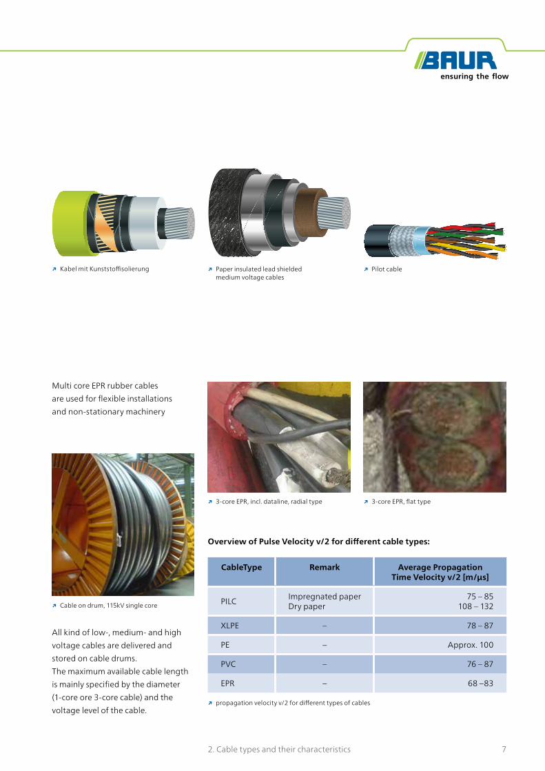
All kind of low-, medium- and high voltage cables are delivered and stored on cable drums. The maximum available cable length is mainly specified by the diameter (1-core ore 3-core cable) and the voltage level of the cable.
Multi core EPR rubber cablesare used for flexible installationsand non-stationary machinery
CableType Remark Average Propagation Time Velocity v/2 [m/μs]
PILC Impregnated paperDry paper
75 – 85108 – 132
XLPE – 78 – 87
PE – Approx. 100
PVC – 76 – 87
EPR – 68 –83
Overview of Pulse Velocity v/2 for different cable types:
↗ 3-core EPR, incl. dataline, radial type
↗ propagation velocity v/2 for different types of cables
↗ Cable on drum, 115kV single core
↗ 3-core EPR, flat type
↗ Paper insulated lead shielded medium voltage cables
↗ Kabel mit Kunststoffisolierung ↗ Pilot cable

8 4. Cable Fault Location Procedure
4. Cable Fault Location Procedure
3. Cable FaultsA cable fault can be defined as any defect, inconsistency, weakness or non-homogeneity that affects the perfor-mance of a cable. All faults in underground cables are different and the success of a cable fault location depends to a great extent on practical aspects and the experience of the operator. To accomplish this, it is necessary to have personnel trained to test the cables successfully and to reduce their malfunctions. The development of refined techniques in the field of high voltage testing and diag-nosis, in addition to the variety of methods for locating power cable faults, makes it imperative that qualified and experienced engineers and service operators be employed. In addition, it is important for the trained personnel to be
thoroughly familiar with the fundamentals of power cable design, operation and the maintenance. The purpose of this document is therefore to be an additional support to the user manuals of the different equipment concerning all aspects of the fault location in order to make up a volume of reference which will hopefully be useful for operators and field engineers. The technology used and the expe-rience that can be shared is based on the BAUR expertise collected over more than 70 years.
The faulty cable respectively phase has to be disconnected and earthed according to the local standards and safety regulation.
Cable fault location as such has to be considered as a procedure covering the following steps and not being only one single step.
▪ Fault Indication ▪ Disconnecting and Earthing ▪ Fault Analyses and Insulation Test ▪ Cable Fault Prelocation ▪ Cable Route Tracing ▪ Precise Cable Fault Location
(Pinpointing) ▪ Cable Identification ▪ Fault Marking and Repair ▪ Cable Testing and Diagnosis ▪ Switch on Power
↗ Grounding of all phases

93. Cable Faults
4.1 Cable Analysis and Insulation Test
In general it is very helpful to start by gathering all avail-able details about the cable network and the cable itself. The characteristics that are influencing the cable fault procedure can be listed as following:
▪ Cable type …what kind of cable sheath? → Individually shielded cores in a 3-core cable → Is it possible that a core – core fault can occur?
▪ Type of insulation material … PE, XLPE, EPR, PVC or PILC; different pulse velocity v/2
▪ Length of the cable under test … make sure no further continuing cable section is connected at the far end!
▪ Is the network including T-branch joint arrangements? Do we know their locations and their individual length?
▪ How is the cable laid? Direct buried, pipe/manhole arrangements, laid in enclosed tranches, how are the tranches designed? Is the cable laid in trays so that it may not be in direct contact with the soil?
All these questions shall be answered before the cable fault location procedure is started. During the explanation of the individual application of methods, the influences of these aspects will be mentioned.
Fault Analyses shall cover ▪ all resistance values
( L1/N, L2/N, L3/N, L1/L2, L2/L3, L1/L3) ▪ all line resistances / confirmation of continuity
If the considered fault is a high resistive or intermittent fault, the next step is to apply a DC voltage to determine the voltage where the fault condition is changing. In high resistive faults, this effect could be that it gets more con-ductive at a certain voltage, or in an intermittent fault the breakdown voltage, where the remaining insulation gap at the faulty joint flashes over. This breakdown voltage shall be noted, as it will be required as minimum voltage value for the following fault location procedure where a surge generator is applied to cause the fault to flash over. Either for prelocation with SIM/MIM, ICM, Decay or finally for the cable fault pinpointing by using the acoustic method. Faults in general are categorized in low resistive and high resistive faults. As shown below, the point of differentia-tion is roughly between 100 and 200 Ohm. Detailed litera-ture on reflectometry is explaining the reason. Around this value, the negative reflection is changing to an impedance characteristic that does not cause a reflection anymore and the TDR pulse is passing by without significant reflection.

10 3. Cable Faults
4.3 Cable Connections HV and MV cables
Connection to pole mounted terminations:
Whenever the connection is done at pole mounted terminations consider the following points:
▪ terminations must be cleaned ▪ operating and safety earth have to be
connected to the common earth point on the pole!
↗ connection to pole mounted cable terminations
4.2 Cable Fault Types
1. Fault between core-core and/or core - sheath: ▪ Low resistive faults (R < 100 - 200 Ω)
→ short circuit ▪ High resistive faults (R > 100 - 200 Ω)
→ Intermittent faults (breakdown or flash faults) → Interruption (cable cuts)
2. Defects on the outer protective shield (PVC, PE): ▪ Cable sheath faults
RL =!C ! lAC
+!S ! lAS
Most of the cable faults occur between cable core and sheath. Furthermore, very frequently blown up open joint connections or vaporized cable sections can cause the core to be interrupted. To figure out whether such a fault is present, the loop resistance test shall be done. By using a simple multimeter, the continuity in general can be measured. The easiest way to perform this test is to keep the circuit breaker at the far end grounded. Corrosion of the cable sheath may increase the line resistance. This is al-ready an indication for possible part reflections in the TDR result. As a rough guidance, a line resistance of 0.7 Ohm/km can be considered as normal condition. In dependence of the fault characteristic, the suitable cable fault preloca-tion and pinpointing methods need to be selected by the operator.

113. Cable Faults
1-phased connection
3-phased connection
Connection of operating and safety earth:
During every test, the two nonconnected cores have to be grounded throughout the tests.
When a three phase cable fault location system is used, all three cores have to be connected.
Protection / Safety earth (transparent or yellow / green) and Operation earth (black) must be connected to a common ground bar! The grounding bar always must be a blank metal bar. Remove any painting and corrosion before connecting the clamps!
↗ single phased connection, not involved phases grounded
↗ 3 phased connection, common grounding point of safety earth and operation earth clamps
Connection to enclosed substations / Compact stations:
For different types of substations, differentadapters have to be used. Make sure thatthe used adapters are in good conditionsand fitting to the bus bars/ termination.Make sure that all neighbouring linesare in a safe distance and proper safetybarriers and signs are placed. Followthe local safety regulations.
↗ connection to enclosed substations

12 3. Cable Faults
4.4 Cable Connections at LV cable networks
In low voltage networks, the connection of the fault location equipment in most cases is applied to the faulty core that is expected to flash over to the ground core. On the other hand, the mains supply is tapped between one healthy core and ground. This may force the operat-ing earth (OE) to rise up to a higher potential than usual. According to this potential lift, the potential of the safety earth (SE) will also increase. Due to this potential lift, a larg-er potential difference and so a higher voltage between neutral wire (connected to OE) and phase will occur, which may cause a harmful effect to the equipment’s mains input.
To prevent any damage to the equipment a separation transformer has to be used.
↗ connection scheme in LV networks
Sheath layer
Grounding connected to cable sheath
Floating mains supply via separation transformer
STG 600OE
SE
L
N
L
N
↗ connection of mains supply by using a separation transformer
By using a separation transformer, the main supply is following the potential lift of the operating earth (OE). It is con-templated as a floating main supply. Therefore overvoltage between earth potential and main supply will be prevented. A separation transformer should also be used in stations with poor grounding conditions. The power supply system will stay stable during all potential lifts caused by poor grounding conditions.

133. Cable Faults
4.5 Grounding conditions
4.5.1 Normal grounding conditions
All high voltage instruments and systems are designed to be operated under field conditions. However, when high volt-age instruments are put in operation, grounding is the most important point. As normal grounding condition, a specific ground resistance of up to 3,3 Ohms is defined. Under these conditions, no additional safety precautions for operators and equipment are required. To improve the safety and to prevent damage to the equipment the following additional features are recommended:
▪ Separation transformer ▪ Earth loop control system (used in cable test vans)
The earth loop control system checks the connection between safety earth and operating earth in the substation. It is ensured that the safety earth and the operation earth clamps are connected properly.
▪ Auxiliary earth control system (used in cable test vans) The auxiliary earth monitoring system is used for potential monitoring of the earth potential at
the test van compared to the substation earth bar. Furthermore the connection of the safety earth lead to the station earth is monitored.
L3
L2
L1
N
H
-
1
23
4
5
6
↗ connection of cable fault location system including earth loop control and auxiliary earth monitoring system

14 3. Cable Faults
4.5.2 Ground conditions with high earth resistance
Sometimes it may happen that the cable fault location equipment has to be connected in the field where no proper sub-station grounding is available. Under the circumstance, that the grounding condition of the grounding system is higher than 4 Ohms it is very important to connect the safety earth (SE) clamp together with the operation earth (OE) to the grounded sheath of the cable under test. Furthermore an earth spike shall be installed nearby the connection point. In very dry sand conditions it is required to use an earth spike of appropriate length to reach the humid soil.
By using a separation transformer, it is possible to create a floating mains supply system. Overvoltage between the earth potential and the mains supplied parts can be prevented.
mainssupply
Grounding connected to cable sheath
Additionalearth spike
Floating mains supply via separation transformer
OE
SE
L
N
L
N
HV
PE
cable testvan
ENSURING THE FLOW
↗ mains supply for cable fault location system with separation transformer; connection in locations with high earth resistance
155. Cable Fault Prelocation
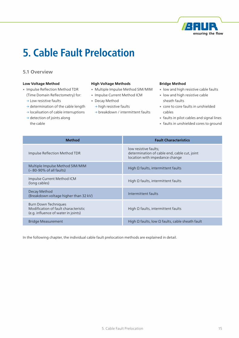
5. Cable Fault Prelocation5.1 Overview
Low Voltage Method ▪ Impulse Reflection Method TDR
(Time Domain Reflectometry) for: → Low resistive faults → determination of the cable length → localisation of cable interruptions → detection of joints along
the cable
High Voltage Methods ▪ Multiple Impulse Method SIM/MIM ▪ Impulse Current Method ICM ▪ Decay Method
→ high resistive faults → breakdown / intermittent faults
Bridge Method ▪ low and high resistive cable faults ▪ low and high resistive cable
sheath faults ▪ core to core faults in unshielded
cables ▪ faults in pilot cables and signal lines ▪ faults in unshielded cores to ground
Method Fault Characteristics
Impulse Reflection Method TDRlow resistive faults;determination of cable end, cable cut, jointlocation with impedance change
Multiple Impulse Method SIM/MIM(~ 80-90% of all faults) High Ω faults, intermittent faults
Impulse Current Method ICM(long cables) High Ω faults, intermittent faults
Decay Method(Breakdown voltage higher than 32 kV) Intermittent faults
Burn Down TechniquesModification of fault characteristic(e.g. influence of water in joints)
High Ω faults, intermittent faults
Bridge Measurement High Ω faults, low Ω faults, cable sheath fault
In the following chapter, the individual cable fault prelocation methods are explained in detail.

16 5. Cable Fault Prelocation
5.2 Impulse Reflection Method (TDR- Time Domain Reflectometry)
The TDR method is the most estab-lished and widely used measuring method for determination of
▪ the total length of a cable ▪ the location of low resistive
cable faults ▪ the location of cable interruptions ▪ the location of joints along
the cable
The Time Domain Reflectometer IRG (BAUR abbreviation for Impulse Reflection Generator) sends a low voltage impulse into the cable under test. The low voltage impulse (max. 160V) travels through the cable and is reflected positively at the cable end or at any cable interruption (cable cut). At a short circuit point this low volt-age impulse is reflected negatively.
The Time Domain Reflectometer IRG is measuring the time between release and return of the low voltage impulse. A change of the impedance in the cable, e.g. a joint, will be displayed as a laid S. The relevant distances are shown by automatic cursor settings to the significant locations in the graph.
↗ schematic diagram of connection of IRG, TDR reflection graphs
Block diagram:
Definition of the Reflection Factor [r]:
r = Z2 ! Z1Z2 + Z1
To enable any pulse to travel along a cable and therefore resulting in a reflection graph, it is required to have a par-allel path of two conductors. The reflection of the impulse is caused by the change of impedance between those two paths. Every interruption, change of impedance or end therefore is indicated. A single core without referring to a second core or to a screen does not fulfil these basic requirements and therefore the TDR Method cannot show any result.

175. Cable Fault Prelocation
Measurement example:
By comparing the TDR graphs of a healthy phase (L1) and a faulty phase (L2) with a short circuit or low resistive fault, the faulty position, is shown as a clear fault at the location where the lines are deviating from each other. The high resolution of the Time Domain Reflectometer enables to set the cursor exactly to the point where the graphs are deviating from each other.
Practical experience showed that sometimes the total ca-ble length is unknown or the cable is consisting of different cable types. In such a mixed cable, the pulse velocity v/2 is uncertain. A cable interruption therefore is getting difficult to prelocate from one single TDR graph.
The practical application of fault location is to perform the prelocation from both cable ends (A and B). When measur-ing from both sides the ideal situation would be that both distances add up to the total cable length. Influenced by the used pulse velocity a certain deviation may be recog-nized. Adding both fault distances to one line equal to the total length two positions is indicated. The real fault dis-tance therefore has to be in between these positions. De-pending on the constellation of cable parts with different pulse velocity, the exact position may not be exactly in the middle of these two positions. Fault pinpointing therefore has to be carried out over a certain distance.
↗ TDR graphs measured from both cable ends, unknown propagation velocity v/2
↗ TDR graph, Comparison of healthy and faulty phase

18 5. Cable Fault Prelocation
5.3 Multiple Impulse Method (SIM/MIM)
The Multiple Impulse Method is the most advanced cable fault prelocation method available. Every cable fault that is either a high resistive or intermittent fault cannot be indicated by means of the TDR method. The low voltage impulse sent out by the Time Domain Reflectometer is not reflected at the faulty position, as the fault impedance compared to the insulation impedance of the healthy part of the cable is not significantly lower.
Based on this fact, the Multiple Impulse Method is sup-ported by a single high voltage impulse that is generated by the coupled surge generator. Like this it is possible to change the high resistive fault temporarily into a short circuit (flash over, temporary low resistive fault condition) and therefore can be detected by a second TDR impulse (SIM) or multiple secondary Impulses (MIM). The low voltage TDR impulse is coupled to the high voltage output of the surge generator via the coupling unit SA32. For many years, the Secondary Impulse Method was consid-ered to be the most advanced method. Problems were figured out, as faults with difficult characteristic had to be located. Those influences like water in a joint, oil-reflow in oil filled cables, etc. either shorten the duration of the flash over or delayed the ignition time of the flash. All these effects are influences that make the timing for the triggering and release of the secondary impulse, to reach the fault exactly at the short time frame of arcing, very difficult. Manual trigger delay settings had to be varied and therefore requested the user’s skills significantly. The meth-od of “try and see” requested to stress the cable by high voltage impulses sent out by the surge generator as every measurement requested a further flash over and therefore HV impulse.
The Multiple Impulse Method is basically the further, much more advanced development of the Secondary Im-pulse Method (SIM). The big advantage reached by means of the MIM is, that a wider timeframe “monitoring” shows the fault condition of such a described fault before, dur-ing as well as after extinguishing of the fault. Therefore, no manual trigger delay time adjustment and “try and see” is requested any more.
The Advanced Secondary Impulse Method (SIM-MIM)
Impulses which are sent out from the Time Domain Reflec-tometer into a cable show no reflection at high impedance cable faults. Therefore the positive reflection of the far cable end is detected. In a second step the fault is ignited by a single high voltage pulse or DC voltage of a surge gen-erator and the discharge shows up as an arc at the faulty spot. Exactly at the time of arcing (short circuit condition) a second measuring pulse sequence is sent from the Time Domain Reflectometer into the cable which is reflected from the arc with negative polarity because the arc is low resistive. The modern Time Domain Reflectometers (IRG 2000 and IRG 3000) are using a 200 MHz transient record-er and send out 5 low voltage impulses considered as the Multiple Impulse MIM (compared to one single secondary impulse SIM) which are reflected at the faulty spot and are recorded individually. The effect of this Multiple Impulse Method is that on one single high voltage impulse, 5 faulty graphs recorded in a sequence are shown. The char-acteristic of the fault is captured as a sequence of snap-shots. The simultaneous display of the condition before the flashover and the condition during the flashover leads to highest precision of fault distance assessment.
↗ Schematic connection for SIM/MIM
l = t ! v2
Block diagram:

195. Cable Fault Prelocation
1 ... not yet arcing2 ... not yet arcing, resistance
condition already changed3 & 4 ... fault arcing5 ... arc already extinguished
↗ measurement graph IRG 3000, SIM/MIM
↗ SIM/MIM graph sequence IRG3000, display of automatically measured multiple sequence
Faulty position
Healthy trace, cable end
Five „faulty“ traces, currently only one is displayed
1
3
2
4 5

20 5. Cable Fault Prelocation
The shown graph sequence is giving an example of a suc-cessful MIM-result on a cable fault in a joint influenced by presence of water causing the flash over to ignite with a delay and to be extinguished immediately. Only by means of a sequence of impulses, a wide enough timeframe can be monitored.
The intensity of the flash over and therefore the possibility to reach a result turns on the energy that can be released. Maximum defined voltage level applicable to the cable may limit the output power of the surge generator. In such a case, if the fault is a flashing fault (that means no leakage current up to certain breakdown voltage - intermittent fault), the cable capacity can be used to store energy and therefore achieve a more intensive flash over. This effect is used by the DC application of the MIM-method.
R
t
Ignition delay
Diff. Trig. Delays
1 2 3 4 5
Flas
h ov
er
High resistive
Short circuit
MIM- illustration
Extin
ctio
n
Water
influence
↗ SIM/MIM graph sequence, reflection of fault influenced by water presence
↗ setting of voltage and selection of voltage range at the surge generator SSG

215. Cable Fault Prelocation
Practical experience:
Certain faults show up the very wet characteristic. Water has penetrated into joints and is influencing the intensity of the flash over. This effect in many cases is the reason why prelocation graphs may not show clear results. Furthermore no clear flash over noise can be heard when the pulse is released by the surge generator. Pinpointing according to the acoustic method is very difficult.
To vaporize the water / humidity out of a joint or cable, the surge gener-ator has to be applied in surge mode for a while. To release the full pulse energy, the surge generator is used directly (without SIM-MIM filter). The high repetitive pulse frequency and high output energy is causing the faulty loca-tion to dry out. With the drying effect the pulse sound is changing. In some situations, it might be requested to continue the pulsing for several minutes. During the pulsing, the Impulse Current measurement can be started. Very often, only when the HV pulse is applied continuously without interruption, the faulty distance can be measured. As soon as the flash over sound is getting a stable metallic sound, the system quickly has to be switched to SIM/MIM and the measurement can be done. Water in the joint may flow back to the dried spot immediately. Therefore, the change to perform the SIM/MIM in some cases needs to be done very quickly. Operators experience and skill enables to locate these kinds of fault more easily. Beside the surge generator, especially in oil filled cables, the burn down transformer is applied for this drying purpose. Today this function is the only remaining application of burn down transformers.
Multiple Impulse Method DC, MIM DC (advanced SIM DC)
The MIM DC Method is operated like the MIM Method based on the surge impulse. To reach a higher surge energy that is defining the flash over inten-sity, the surge generator is used in DC mode. Like this the surge generator’s capacitor is switched in parallel to the cable. Both, the surge generator’s and the cable’s capacity are charged simultaneously and the applied surge capac-ity is increased. Especially for long cables the cable capacity that is very much depending on the break down voltage can be very high and leading to proper results.

22 5. Cable Fault Prelocation
Surge generator range setting
The output energy that can be sent out by the surge generator is basically depending on the capacity C of the integrated capacitor bank. The energy stored in a capacitor is defined by the charging voltage. According to the following formula and the enclosed table, the output energy is shown in relation to the different available voltage ranges. The energy of a high voltage impulse is defining the intensity of the flash over at the faulty point. This value is very important to reach a stable flash over used for SIM/MIM or Impulse Current Method during prelocation as well as for pinpointing according to the acoustic method. The higher the discharge energy the louder the flash over is.
Example of available Surge Energy in different Voltage Ranges and applied Charging Voltages:
Surge generator 32 kV, SSG 2100 ▪ 2048 Joules ▪ voltage ranges 0-8 kV, 0-16 kV and 0-32 kV ▪ consists of four capacitors connected
either in line or in parallel
C = 2 !EU 2
C = 2 !2048J(16.000V )2
=16µF
Charging voltage
32 kV range
16 kV range
8 kV range
32 kV 2048 J – –
16 kV 512 J 2048 J –
8 kV 128 J 512 J 2048 J
↗ Internal capacitor alignment in different selectable voltage ranges of SSG Surge Generator (8 kV, 16 kV and 32 kV)
E = C !U2
2
16kV range:

235. Cable Fault Prelocation
5.4 Impulse Current Method (ICM)
The previously mentioned cable fault prelocation methods based on a TDR impulse are in general affected by either damping of the signal in very long cables or by part reflections at joints along the cable. These unusual damping influenc-es can be caused due to corrosion of the cable sheath or any other influence in the joint causing an influence to the length resistance. In very long cables the natural damping of the cable may cause the TDR impulse to be damped off before returning to the Time Domain Reflectometer and therefore cannot be applied successfully.
To cover the application of cable fault prelocation under such conditions, the Impulse Current Method (ICM) can be applied. Basically a surge generator releases a HV impulse that is flashing over at the faulty location. This discharge causes a transient current wave travelling along the cable sheath between the surge generator and the flashover point. The repetition interval of this pulse is determined as the faulty distance. As a coupling unit, an inductive coupler (SK1D) is connected to the sheath of the SSG output cable. The Time Domain Reflectometer IRG 2000 or IRG 3000 are operated with automatic adjustment of all settings and lead to proper recordings. As the pulse width of the transient current pulse is very wide, the accuracy of the ICM method is very high in long cables. In short cables the transient pulses are influencing each other.
The Impulse Current Method is detecting the current impulse traveling along the cable sheath during flash over. The sequence of the current impulse is measured via the inductive coupling unit SK 1D. Every impulse is reflected at the end or fault with the reflection factor depending on the resistance at this point related to earth. Every change in current direction of the reflected impulse is detected via the inductive coupling unit SK1D. As shown below, the first impulse reflection is influenced by the ignition delay time of the flashing fault. For distance determination, the distances between the 2nd to 3rd or 3rd to 4th impulse shall be con-sidered. By means of the known impulse velocity v/2 of the individual testing cable and the periodical time of the reflected wave, the faulty distance is calculated by the IRG. The distance to the faulty point can be measured by setting the cursors according to the regularity of the positive wave peaks in the picture. In practical measurements the voltage is increased so that a breakdown is created. The discharging impulse is then traveling between the arcing spot and the surge generator until it is discharged to ground.
↗ schematic connection for ICM
↗ measurement graph IRG 3000, ICM
l = t ! v2

24 5. Cable Fault Prelocation
Sequence of reflection (ICM):
The pulse polarity of the recorded pulses is depending on the direction of the coupling coil. The indicated pulse sequence already shows the inverted positive impulses. By add-ing the reflection factors (r = - 1, HV source SSG and r = - 1, cable fault) the pulse sequence is created as follow-ing.
1 The pulse is released by the Surge Generator SSG. The sent out impulse is negative (1st pulse recording). From the faulty point it returns as a positive pulse.
2 When arriving at the SSG, it is reflected and running backwards as a negative impulse (2nd pulse recording). At the flash over point, the pulse is reflected again, and returning as positive pulse.
3 When arriving at the SSG, the pulse is reflected again and trig-gering as another negative pulse. This procedure carries on until the pulse is damped away.
The reason for this reflection se-quence is that in this case both ends are low resistive points of reflection. As both reflection points (faulty point and SSG) are negative reflec-tion points, theoretically the impulse would be doubled every time. Due to natural damping influences in every cable, the impulse is damped and the useful reflection frequency is limited with 4 to 5 time intervals. To enable the display of several reflection peri-ods it is important to use a view range setting equal to 2 to 3 times the total cable length.
↗ pulse sequence of transient pulse, ICM
r = Z2 ! Z1Z2 + Z1
1 2 3

255. Cable Fault Prelocation
↗ schematic connection, Decay method
↗ measurement graph IRG3000, Decay method
5.5 Decay method
The previously explained SIM/MIM and ICM methods are based on the surge generator SSG. All kind of cable faults with a breakdown voltage of max. 32kV can be prelocated successfully.
The application of cable fault location even in high voltage cables like e.g. 66kV, 115kV, 132kV, 220kV etc. in general also do show a fault breakdown voltage below 32kV. The experience show, that these cables are operated on rather high loads and the breakdown energy in the event of cable fault is so high, that the fault condition is burnt down heavily. Especially XLPE cables do show up this effect. Therefore the majority of cable faults even in high voltage XLPE cables can be located by means of a 32kV based cable fault location system.
Certain circumstances may cause the fault to remain as an intermittent fault with a breakdown voltage higher than the rated voltage of a surge generator. For these cable faults, the Decay method can be applied. To reach the breakdown voltage a DC or VLF source is used as a basic instrument.
The Decay method is based on voltage decoupling by a capacitive voltage divider. The faulty cable is charged by applied VLF / DC voltage up to the breakdown level. As the cable is a capacitor a high energy can be stored in the cable. When reaching the breakdown voltage, the break-down creates a transient wave travelling between the faulty point and DC source. This transient wave is recorded by the Time Domain Reflectometer IRG via the capacitive voltage divider CC1. The recorded period of oscillation is equal to the distance to the fault. Compared to the ICM method, the Decay method is based on a transient voltage wave continuously recorded by a capacitive coupler.

26 5. Cable Fault Prelocation
Sequence of reflection (Decay Method)
By adding the reflection factors (r = + 1, HV source and r = - 1, cable fault) the pulse sequence is defined as following: The cable is charged with negative voltage.
1 The flash over causes a positive discharge transient wave (1.1) that is travelling to the near end.
2 At the HV source the pulse is re-flected without a polarity change. (1.2).
3 Arriving at the flash over point again (1.3) the transient pulse is reflected and the polarity is changed. The pulse is negative.
4 Arriving at the HV source, the pulse is reflected (1.4) again with-out a polarity change.
5 At the flash over point the pulse is reflected again with a polarity change (2.1) and the sequence is repeated again. This proce-dure carries on until the pulse is damped off.
1.1 – 1.4 … first sequence2.1 – 2.4 … second sequence3.1 – 3.4 … third sequence
12
34
5
One recorded pulse cycle (e.g. positive peak to positive peak or ramp to ramp) is representing four times the travelling distance of the pulse. There-fore for the Decay method, automati-cally the distance calculation is based on the formula:
l = t ! v4
To enable the display of several reflection periods it is important to use a view range setting equal to 2 to 3 times the total cable length. Due to damping reasons, under certain circumstances, the delivered graph for either the ICM or the Decay method may be difficult to evaluate.
Damping and part pulse reflection cause the transient signal recording to appear with additional spikes and/or highly flattened characteristic.
For such difficulties, the following explained Differential methods are useful to come around these influences.

275. Cable Fault Prelocation
5.6 Differential Impulse Current Method / Differential Decay Method
Basically for these methods one healthy auxiliary core is required. The coupling unit for both, the Differential Im-pulse Current Method and the Differential Decay Method the 3phased surge coil SK3D is used as a coupler. As the HV need to be applied to two cores simultaneously, these methods are used only in combination with 3phased cable test vans. The coupling coil is mounted, so that all three cores L1, L2 and L3 are contacting the triangular shaped 3phased coupler on one edge each. Independent which two phases are selected, the remaining signal recorded is the differential signal coupled.
In a first step the HV impulse is released into the healthy core and the faulty core simultaneously. The recorded signal will show up the first differential picture. In a second step, at the cable end, the two cores are linked togeth-er. Therefore the effective length of the healthy core is extended with the length from the far end to the faulty position in the faulty core. As this reflection characteristic is now different compared to the open end in the first step,
the impulse is reflected differently, whereas the reflection taking place in the faulty core stays the same. Due to phys-ical extension of the healthy core in the second step, also the resulting differential picture appears different. Laying both graphs on top of each other the deviation point that is influenced by the extension of the healthy core to the fault, shows the faulty distance from the far end. Certain software supported settings enable to see a very clear fault position. The graphs recorded during both, the Differen-tial Impulse Current Method and the Differential Decay method are not depending on the damping influences. As this method is using the feature of measuring a differen-tial value, in-continuities in the cable resulting as spikes in the graph are substituting each other and therefore are eliminated.
The Differential Impulse Current method is applied similar to the ICM on intermittent and high resistive faults with a breakdown voltage of up to 32 kV. The high voltage source is the surge generator.

28 5. Cable Fault Prelocation
The Differential Decay method is working similar to the Decay method and is applied on intermittent faults with break-down voltage above 32 kV. As voltage source, any VLF or DC test instrument is used.
The Differential Impulse Current Method and the Differ-ential Decay Method are based on the current impulse pick up via an inductive coupling unit. For the Differential Decay method, the faulty cable is charged by applied DC or VLF voltage up to the level of the breakdown, whereas for the Differential Impulse Current Method a surge energy impulse is used. This breakdown causes a transient wave which is travelling between the faulty point and the sys-tem. This transient wave is recorded by the Time Domain Reflectometer IRG 3000 via the inductive coupling unit.
The Differential Impulse Current Method and the Differen-tial Decay Method are working with two separate meas-urements (one without Bypass Bridge and a second one with a Bypass Bridge at the far end). At the splitting point of these two recordings, the faulty position is indicated.The information of the distance to the faulty position is the fault distance related to the far end!
↗ Schematic connection for Differential Impulse Current Method
↗ measurement graphs IRG3000, Diff. ICM method; 1st and 2nd measurement, indication of fault distance from the far end
Für Druck zu niedrig aufgelöst
Für Druck zu niedrig aufgelöst

295. Cable Fault Prelocation
↗ IRG 3000 19“ Version ↗ IRG 2000
Unique features IRG 3000 – IRG 2000:Real time sampling rate: 200MHzAutomatic parameter settingAutomatic cursor settingCFL – prelocation methods: TDR, SIM/MIM, ICM, Decay
Differences between IRG 3000 – IRG 2000:
IRG 3000 IRG 2000
3-phased Echometer 1-phased Echometer
Option: Computer controlled MOhm-Meter –
Measuring range > 200 km 65 km
Max. pulse voltage 160 V 65 V
Large 15,1” LCD TFT display 6” LCD display
Memory > 100.000 files 100 files

30 5. Cable Fault Prelocation
5.7 Bridge Method
All faults having the characteristic to happen between two defined cores and therefore two parallel wires can be prelocated with any of the previ-ously mentioned cable fault preloca-tion methods based on pulse reflec-tometry. Certain cable structures enable cable faults to happen from a core to the outside and therefore the soil. Especially in unshielded cables that can either be high voltage DC cables used for railway supply, low voltage cables or also signal cables or so called pilot cables, faults mainly happen between a core and the sur-rounding soil. As the related medium in that case cannot be accessed like a grounded metal sheath, the theory of reflectometry is no more working.
An impulse only can travel, as long as the two parallel conductive paths are given. Cable sheath faults, that are defects in the outer protec-tive PVC insulation, are showing the same electrical image like the above mentioned faults. Cable sheath faults do not directly influence the electri-cal performance of a shielded cable, but do have a negative side effect in medium term operation of the cable. The damages of the outer sheath enable water from the surrounding soil to penetrate into cable. Corrosion of the cable sheath as well as develop-ment of water trees will lead to break-downs sooner or later. Therefore, according to IEC 60229, protective over-sheaths have to be tested and
faults shall be repaired to ensure the long term performance of the cable. These kinds of cable faults can only be prelocated by using a measuring bridge.
Bridge methods are basically used for prelocation of low resistive faults. By using a high voltage source that is integrated in the latest generation of measuring bridge instruments even high resistive faults can be prelocat-ed.
All bridge measurement methods that work with direct current for locating faults in cables (Glaser and Murray) are based in principle on modified Wheatstone circuits.
5.7.1 Principle of the Wheatstone circuit
The bridge is balanced when points (a) and (b) are subject to the same potential. In this situation, the galvanometer shows zero. Points (a) and (b) are at the same potential when the following condition is fulfilled:
R1R3=R2R4
resp.
R4 =R2 !R3R1
If R4 is the resistance RX being sought then RX can be defined as:
RX =R2 !R3R1
↗ Wheatstone circuit

315. Cable Fault Prelocation
5.7.2 Measuring circuit according to Murray
The measuring bridge circuit according to Murray is ap-plied on arrangements, where beside the faulty core, one healthy core with same diameter and conductor material is present. This circuit of the external loop comprises the back and forth wire as well as the resistance created via the linking bridge at the end. Therefore, the linking bridge between the cores is an essential part of the circuit and has to be close to zero ohms.
↗ Murray – Balancing Circuit
↗ Murray – Measuring Circuit
↗ measuring circuit according to Murray
The degree of precision of the bridge depends on the following factors:
▪ The bridge current ▪ The loop resistance of the cable loop ▪ The matching for power transfer of the internal imped-
ance of the galvanometer to the bridge resistance ▪ The sensitivity of the galvanometer ▪ Linearity of measuring potentiometer
32 5. Cable Fault Prelocation
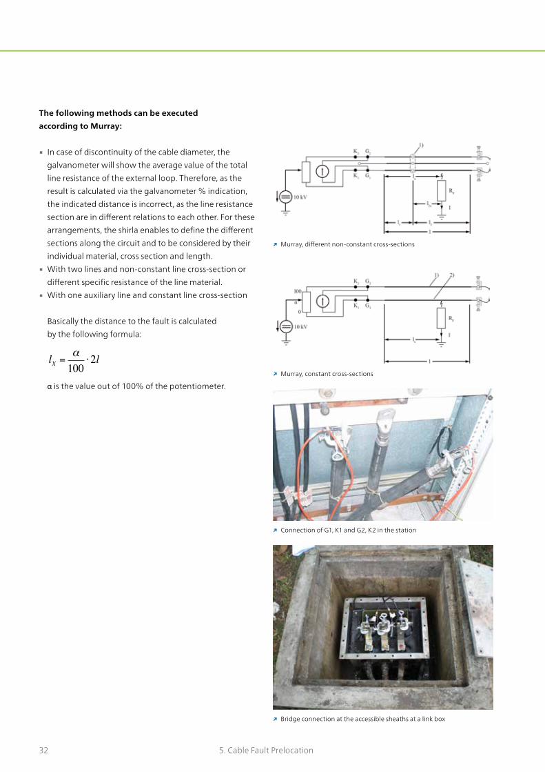
The following methods can be executed according to Murray:
▪ In case of discontinuity of the cable diameter, the galvanometer will show the average value of the total line resistance of the external loop. Therefore, as the result is calculated via the galvanometer % indication, the indicated distance is incorrect, as the line resistance section are in different relations to each other. For these arrangements, the shirla enables to define the different sections along the circuit and to be considered by their individual material, cross section and length.
▪ With two lines and non-constant line cross-section or different specific resistance of the line material.
▪ With one auxiliary line and constant line cross-section Basically the distance to the fault is calculated by the following formula:
lX =!100
!2l α is the value out of 100% of the potentiometer.
↗ Murray, different non-constant cross-sections
↗ Murray, constant cross-sections
↗ Connection of G1, K1 and G2, K2 in the station
↗ Bridge connection at the accessible sheaths at a link box
335. Cable Fault Prelocation
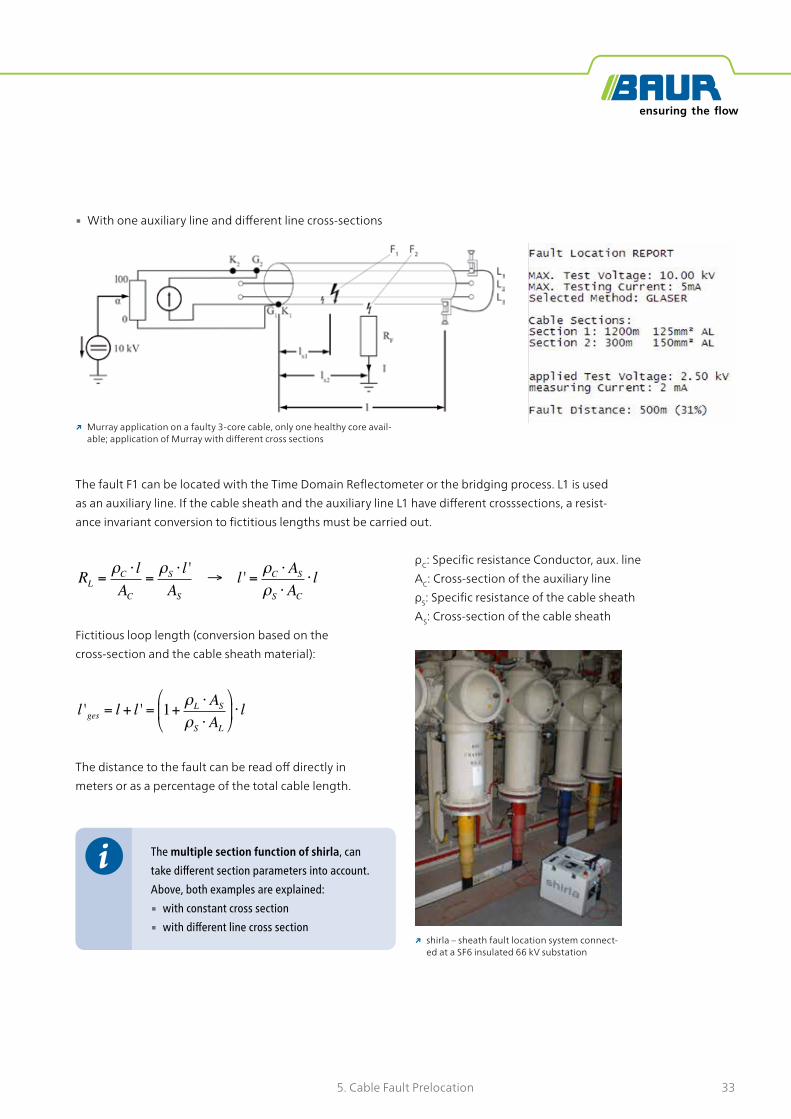
↗ Murray application on a faulty 3-core cable, only one healthy core avail-able; application of Murray with different cross sections
↗ shirla – sheath fault location system connect-ed at a SF6 insulated 66 kV substation
▪ With one auxiliary line and different line cross-sections
The fault F1 can be located with the Time Domain Reflectometer or the bridging process. L1 is used as an auxiliary line. If the cable sheath and the auxiliary line L1 have different crosssections, a resist-ance invariant conversion to fictitious lengths must be carried out.
RL =!C ! lAC
=!S ! l 'AS
" l ' = !C !AS!S !AC
! l
Fictitious loop length (conversion based on the cross-section and the cable sheath material):
l 'ges = l + l ' = 1+ !L !AS!S !AL
"
#$
%
&'! l
The distance to the fault can be read off directly in meters or as a percentage of the total cable length.
The multiple section function of shirla, can take different section parameters into account. Above, both examples are explained:
▪ with constant cross section ▪ with different line cross section
ρC: Specific resistance Conductor, aux. lineAC: Cross-section of the auxiliary lineρS: Specific resistance of the cable sheathAS: Cross-section of the cable sheath
34 5. Cable Fault Prelocation
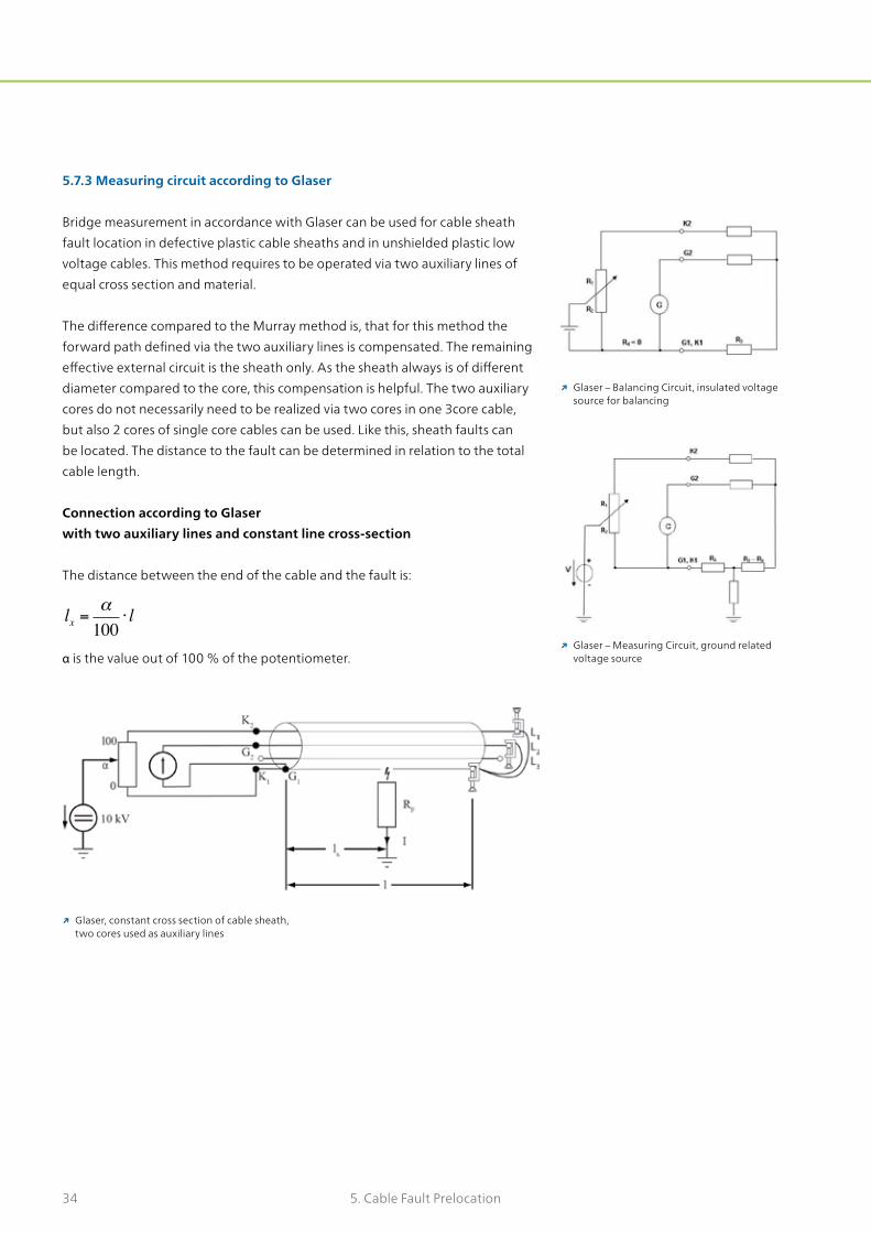
5.7.3 Measuring circuit according to Glaser
Bridge measurement in accordance with Glaser can be used for cable sheath fault location in defective plastic cable sheaths and in unshielded plastic low voltage cables. This method requires to be operated via two auxiliary lines of equal cross section and material.
The difference compared to the Murray method is, that for this method the forward path defined via the two auxiliary lines is compensated. The remaining effective external circuit is the sheath only. As the sheath always is of different diameter compared to the core, this compensation is helpful. The two auxiliary cores do not necessarily need to be realized via two cores in one 3core cable, but also 2 cores of single core cables can be used. Like this, sheath faults can be located. The distance to the fault can be determined in relation to the total cable length.
↗ Glaser – Balancing Circuit, insulated voltage source for balancing
↗ Glaser – Measuring Circuit, ground related voltage source
↗ Glaser, constant cross section of cable sheath, two cores used as auxiliary lines
Connection according to Glaser with two auxiliary lines and constant line cross-section
The distance between the end of the cable and the fault is:
lx =!100
! l
α is the value out of 100 % of the potentiometer.

355. Cable Fault Prelocation
The sequence of measurement: for Murray- and Glaser method
For both measuring circuits, the measurement is carried out in two steps:
1st Step: Balancing of the bridge:By means of the integrated low voltage DC source (not related to ground) the measuring circuit is balanced. Therefore the internal potentiometer is adjusted, so that the equation is fulfilled. The galvanometer is adjusted to zero (α = 0). R4 in the balancing step is defined zero, because the voltage source applied is not related to ground and the fault is not causing any leakage current.
2nd Step: Measurement:For the measurement a ground related DC voltage source is applied and the internal battery used for balancing is switched apart. Therefore the current is now forced to return to the ground potential of the power source. The resistive fault is now coming on stage and the bridge circuit is changing. Depending on the location of the fault, the circuit part R3 as balanced is now splitting up to R3` and R4. The galvanometer is getting out of balance and showing a certain value that is finally corresponding to R4 and therefore the faulty distance. The difference between the Murray and Glaser methods are only the way of connec-tion and the difference in the formula used for distance calculation. The internal bridge circuit of the instrument is not changing at all.
The accuracy of the measurement is mainly depending on the measuring cur-rent that can be forced to flow. For high resistive faults, the required measuring current (5mA = 0.1% accuracy) can only be reached by using a high voltage source. The cable sheath testing and fault location system shirla is operated with an integrated 10kV DC source. Therefore even high resistive faults can be located precisely.
shirla - All in One, all you need ▪ Cable sheath testing
→ up to 10kV ▪ Fault pre-location via integrated measuring bridge
→ up to 10kV ▪ Sheath fault pin-pointing via step voltage method
→ up to 10kV
R1R3=R2R4
↗ shirla - display of fault distance indicated in[m] and([%]), language neutral menu control; automatic measuring sequence
↗ shirla (SHeath, Insulation test, fault Resistance and Location Analyzer)

36 5. Cable Fault Prelocation
5.8 Burn Down Technique
High resistance cable faults lead to very small or even no impedance changes at the faulty spot. Therefore the pulse reflection method TDR is not suitable for location of this fault type. For many years powerful burn down units had been used success-fully for treatment of high resistance cable faults in paper mass impregnat-ed cable (PILC).
The high voltage burn down unit treats the fault by forcing a high current and carbonizes the insulation material. This carbon link is chang-ing the fault to become low resistive and therefore can be prelocated
with a Time Domain Reflectometer IRG according to the pulse reflection method TDR.
Nowadays, fault burning is main-ly used on paper-oil impregnated cables.
Depending on cable insulating mate-rial the burn down procedure can be interfered by reinsulating (melting) or self-extinguishing plastic materials. Even water in joints may influence the burn down method. Fault burning makes the fault condition become low resistive and therefore the appli-cation of the acoustic method for
pin-pointing can be very difficult or even impossible. Nowadays the Multiple Impulse Method and the Impulse Current Method are substi-tuting the fault burning.
↗ ATG 6000 Burn Down Transformer
↗ STG 600 combined with IRG 2000 ↗ Syscompact 2000 M combined with IRG 2000
5.9 Cable Fault Location Systems
5.9.1 Fault location system for low voltage networks– STG 600 / 1000
Cable testing, prelocation and pin-pointing
Test voltage up to 5 kVPulse voltage up to 4 kVEnergy up to 1000 J
Prelocation methods: ▪ TDR 1phased ▪ SIM/MIM
5.9.2 Fault location system for medium voltage networks– Syscompact 2000 M
Cable testing, prelocation and pin-pointing
Voltage range 8/16 kV adjustable in 0,1 kV stepsEnergy 1000JWeight ~85 kg
Prelocation methods: ▪ TDR 1phased ▪ SIM/MIM ▪ ICM

375. Cable Fault Prelocation
5.9.3 Fault location systems for medium voltage networks– Syscompact 2000 / 32 kV – Syscompact 3000 / 32 kV
Cable testing, prelocation and pin-pointing
Voltage range: 8/16/32 kVstepless adjustableEnergy up to 3000 J
Prelocation methods: IRG 2000 ▪ TDR 1phased ▪ SIM/MIM ▪ ICM ▪ Portable version ▪ Version with 25/50 m cable
Prelocation methods: IRG 3000 ▪ Resistance measurement ▪ TDR 3phased ▪ SIM/MIM ▪ ICM ▪ Decay in combination with PGK or VLF ▪ Combination with VLF Testing and Diagnostic TD/PD
↗ Syscompact 2000/32: portable version and vehicle mountable version
↗ Syscompact 3000, Combination of Cable Fault Location, VLF Testing and TD PD Diagnostic mounted in 3t van

38 6. Cable Route Tracing
6. Cable Route TracingCable route tracing is applied to determine the exact route of the underground cable. Depending on the availability of cable laying maps, route tracing is of very high importance as prior step to cable fault pin-pointing. Route tracing can be performed either active or passive. At live cables the harmonics of the mains frequency can be heard as ‘mains hum’. However, all grounded conductors, water pipes and parallel running cables which are connected to the 50 Hz mains system also have this ‘mains hum’. To avoid confusion, it is recommendable to disconnect the conductor and feed the cable with an audio frequency to per-form an active cable route tracing.
6.1 Coupling of Audio Frequency Signal
Galvanic connectionAs far as this method can be applied, galvanic coupling is always the best meth-od for cable route tracing. By direct galvanic connection the ideal signal values can be obtained.Too high signal current might cause the signal to be induced to thesurrounding lines too.Certain circumstances, where the total signal is returned might be difficult to detect. If the input signal running through the cable is returning over the same cable’s sheath, the resulting signal is abolished to nearly zero. The way of connection in such a case is to conduct the inverse current artificially via any other earth path back to the audio frequency generator.
Inductive connection with current clip-on device (AZ 10)The clip-on device can be applied on dead cables if the termination is not accessible (house connec-tion, water, telephone, gas), as well as on live cables for route tracing.
Inductive connection with frame antenna (RA 10)The RA 10 frame antenna is designed for inductive audio frequency signal feeding into metallic pipes and lines which are not accessible. The loop antenna RA 10 is used together with the Audio Frequency Transmitter TG 20/50 and is positioned above the cable. This way of signal coupling can also be used for rout-ing, cable tracing, and terrain examination as well for location of water pipes with rubber joints.
↗ galvanic connection of audio frequency generator TG
↗ galvanic connection ↗ inductive connection via CT clamp AZ 10
↗ inductive connection via frame antenna RA 10

396. Cable Route Tracing
↗ Maximum method
↗ Minimum method
↗ Depth determination
↗ Cable Locator CL20
6.2 Signal detection
Above the ground, the electromagnetic signal transmitted via the audio fre-quency generator can be measured along the cable trace. Depending on the pick-up coil direction, the signal can be coupled differently.
Maximum methodThe detecting coil is horizontal to path of line. Maximum audio signal is direct-ly above the line. The maximum method is used for cable routing as well for terrain examination.
Minimum methodThe detecting coil is vertical to the path of the line. The minimum audio fre-quency signal is directly above line. The minimum method is used for depth determination measurement as well for exact cable tracing and pinpointing.
Depth Measurement according to the Minimum MethodFor the depth determination with a simple surge coil, the characteristic of an isosceles triangle
▪ first determine the exact position of the cable ▪ subsequently, the coil has to be rotated to 45° ▪ The minimum audio-frequency signal is heard at
the depth “d” at a corresponding distance from the path of the cable.
Instruments designed specifically for route tracing are operated with two integrated antenna covering the functions of minimum and maximum method as well as depth determination.

40 6. Cable Route Tracing
Terrain examinationAnother application where the cable locating set can be applied is the so called terrain examination. The signal is injected into the soil via two earth spikes. In case there is any metallic conductor, the signal will return along the conductor. The electromagnetic signal along the conductor can be detected and the con-ductor can be found.
To examine a particular area for existing cable/pipes system, the following procedure is recommended:
▪ dividing the area into squares of approx. 25x25 m ▪ the audio frequency generator has to be set up in the centre of the cable run ▪ the ground rods need to be set into the ground to the left and right of the
generator at approx. 12 to 15m ▪ the output power of the generator is kept low
If there is a metallic conductor within the set out area, it will propagate a mag-netic field in its vicinity. The magnetic field has in most cases the shape of a sin-gle-sided maximum; e.g. with a steep edge to the audio frequency waveform.
↗ connection for terrain examination
↗ signal shape, terrain examination
6.3 Selection of Audio Frequency
Every audio frequency generator is offering the possibility to select different signal output frequen-cies. The different characteristic of the frequencies is the induction effect. The induction of a signal into a neighbouring metal conductor is increasing with the frequency.
- The higher the frequency, the higher the inductive coupling effect
Basically the frequency has to be selected as following:
Low frequency e.g. 2kHz: ▪ for galvanic signal coupling ▪ the signal induction to other cables and pipes can be minimized
High frequency e.g. 10kHz: ▪ for inductive signal coupling with current clamp or frame antenna ▪ high inductive coupling effect is required to couple the signal into the cable

417. Cable Fault Pin-Pointing
↗ signal pick up set UL30 / BM30
↗ schematic connection and shape of acoustic signal – acoustic fault location
↗ magnetic signal along the whole cable, acoustic signal at point of flashover
↗ Cable fault, 1-core 11 kV joint failure
7. Cable Fault Pin-Pointing7.1 Acoustic Fault Location
7.1.1 Acoustic Fault Location in direct buried cables
For pin-pointing of high resistive and intermittent faults in buried cables the acoustic method is used to pin-point the exact fault location. As signal source, a surge generator is used in repetitive pulsing mode. High energy pulses which are released by a surge generator (SSG) force a voltage pulse to travel along the cable. At the fault the flashover happens. This causes a high acoustic signal that is locally audible. Depending on the pulse energy, the intensity of the acous-tic signal varies. These noises are detected on the ground surface by means of a ground microphone, receiver and headphone. The closer the distance from the fault to the microphone, the higher is the amplitude of flashover noise. At the fault position the highest level of flashover noise can be detected.
Propagation Time MeasurementThe acoustic fault location set comprising the receiver UL30 and the ground mi-crophone BM 30 offers the special feature of digital propagation time – distance measurement.
Firstly, the ground microphone is measuring the electromagnetic signal that can be recorded all along the cable where the HV impulse is travelling before finally flashing over at the faulty position. As this signal is available all along the cable trace towards the fault, it can further be used to make sure that the “cable trace” is followed. The maximum signal confirms to be directly above the cable.
Secondly the ground microphone will receive the flashover noise next to the fault on the ground surface as soon as the very close area around the fault is reached.

42 7. Cable Fault Pin-Pointing
Therefore, every flashover activates two trigger situations.
– Magnetic Trigger and Acoustic Trigger
The two signals are of different propagation velocity. Further the distance to the fault influences the difference in trigger of acoustic trigger compared to the trig-ger of the electromagnetic signal. As soon as the magnetic trigger is reacting on the bypassing HV impulse in the cable underneath, a timer is started. When the ground microphone receives the delayed acoustic signal, the measuring cycle is stopped.
The receiver UL automatically indicates the measured time distance (propa-gation time) to the fault via a digital meter indication. According to the meter indication, the faulty position, where the distance indication is lowest, can be found.
By means of the audible acoustic signal the final exact location of the cable fault can be determined. This special feature increases the performance compared to convenient acoustic pick-up sets, as the magnetic indication offers an integrat-ed tracing feature.
↗ UL30 display, indication of magnetic and acoustic signal, indication of distance to fault
↗ field application acoustic fault location
↗ manhole arrangement, cable laid in PVC pipe, acoustic signal only audible on manhole cover
↗ UL30 display, manhole mode, display of two propagation time values used for distance calculation
7.1.2 Pin-pointing of cable faults in pipe arrangements
When cables are laid in pipes the acoustic signal is no more audible right above the cable fault. The acoustic signal in that case is travelling through the air in the pipe and therefore only audible at both ends of the pipe or on the manhole cov-ers. By means of the previously carried out cable fault prelocation, the section of pipe can be determined. Up to today, the final step to determine the exact fault position in the pipe was very difficult or by most pick-up sets impossible. The latest model of pick-up set UL/BM therefore uses a special feature to determine the exact fault position also in manhole arrangements.
Acoustic Fault Location at ManholesFor this method, no additional instrument is requested. Every latest UL receiv-er offers the mode of pinpointing in manhole arrangement. In a first step, the ground microphone is placed on the first manhole cover, where the acoustic sig-nal and the magnetic signal are shown up in a certain propagation time value. By confirming the signal, this value is stored in the receiver. In a second step, the ground microphone is placed on the second manhole cover. Also at this loca-tion, the ground microphone can pick-up an acoustic signal and the magnetic signal that is showing up in a second propagation time value. By entering the distance between the manholes, via the propagation time ratio over the dis-tance, the direct distance to the fault in the pipe is indicated.

437. Cable Fault Pin-Pointing
7.2 Fault Pin-Pointing of Low Resistive Cable Faults
Cable faults that are showing up in a solid grounded condition do not enable to create a flashover at the faulty point by means of a surge generator. There-fore also no acoustic signal is audible and the cable fault pinpointing according to the acoustic fault location is not possible. This condition is mainly resulting from a completely burnt cable fault that is furthermore also low resistive to the surrounding soil. These kinds of cable faults can be pinpointed by means of the step voltage method explained below.
Faults in low voltage cables as well as pilot cables (signal lines) are often difficult to be pin-pointed, because the maximum voltage that may be applied to these cables does not enable to force sufficient surge energy to create a strong flashover that can be pinpointed by means of the acoustic method. As these cables are mainly unshielded, the fault in most cases also appears towards the surrounding soil. Also here, the step voltage method is the suitable pin-point-ing method.
Another difficult fault condition to pin-point in low voltage cables is if the fault is not related to ground and therefore only showing up between two cores. For these conditions, the Twist Method enables successful pointing out the fault.
The 3rd fault type showing similar conditions is the cable sheath fault. A fault in the outer protective PVC insulation of a XLPE cable cannot be located via the acoustic method, as no defined potential point, where the flashover can take place, is given. Here, also the step voltage method enables the localisation. This method also enables to locate several sheath fault locations along a cable.
↗ step voltage method, two earth probes connected to UL30 receiver
↗ discharge of HV pulse; voltage drop in shape of a voltage gradient, zero position above the fault, step voltage can be measured at the surface

44 7. Cable Fault Pin-Pointing
7.2.1 Step Voltage Method
Pin-Pointing of: ▪ Any earth contacting low resistive faults ▪ Cable Sheath Fault
As a signal source, a high voltage impulse sequence or impulse block sequence is sent into the cable under test. The HV pulse is discharged via the resistive fault to the surrounding soil without a flashover. The voltage drop into the soil at the fault location results in a voltage gradient, which can be measured by means of the step voltage method. By using two earth probes, the voltage distribution field is indicated. The multifunctional receiver UL indicates the positive or neg-ative voltage (left or right side from the fault location) via a bar graph as well as an acoustic tone. As soon as the earth sticks are placed symmet-rical above the fault, the resulting voltage is zero and the fault position is determined.
Suitable HV signal sources: ▪ SSG / STG surge generators ▪ shirla - Cable and Cable Sheath
Fault Location System ▪ Any BAUR VLF generator with cable
sheath fault function
Suitable receivers: ▪ UL of latest version in combination
with cable sheath fault location accessories ▪ KMF 1 in combination with cable sheath fault location accessories
In case of multiple sheath faults, e.g. 3 faults, all faults can be located as explained above during one passage over the cable route. This requires appropriate practice and one should know that the step voltage shows several points of po-larity change that might irritate (5 positions with polarity change).
↗ multiple sheath fault can be determined in one sequence, several zero points indicated
457. Cable Fault Pin-Pointing
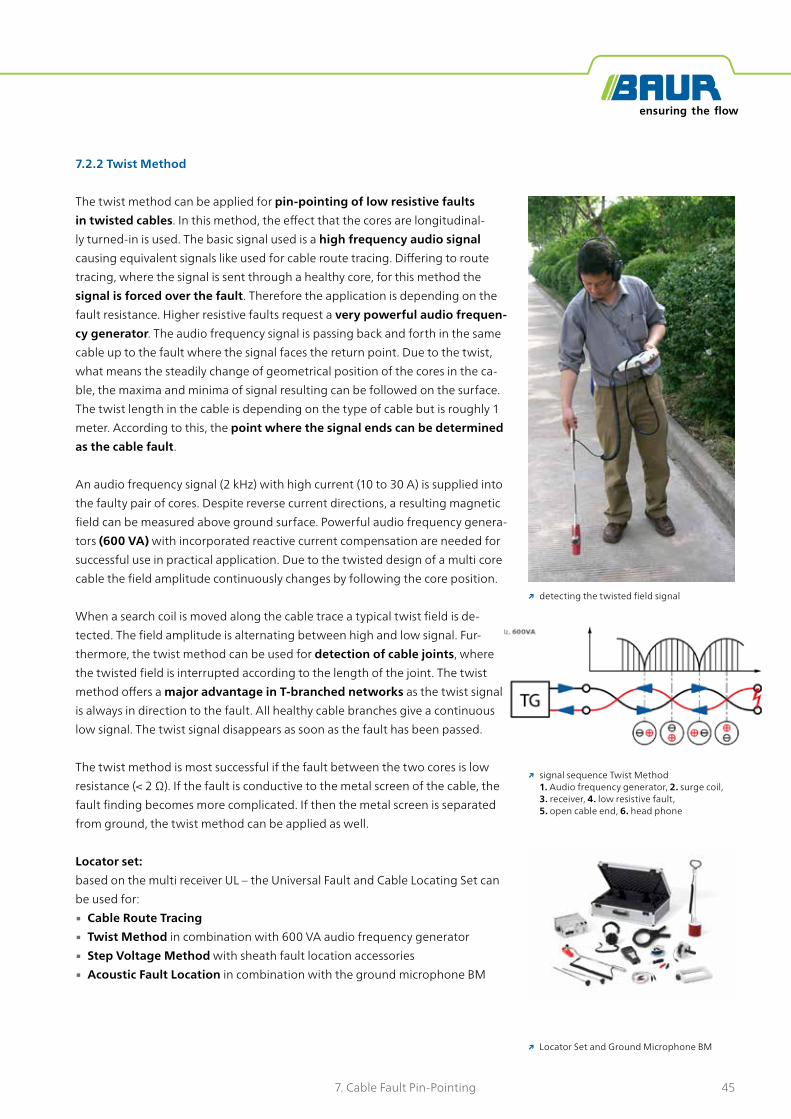
7.2.2 Twist Method
The twist method can be applied for pin-pointing of low resistive faults in twisted cables. In this method, the effect that the cores are longitudinal-ly turned-in is used. The basic signal used is a high frequency audio signal causing equivalent signals like used for cable route tracing. Differing to route tracing, where the signal is sent through a healthy core, for this method the signal is forced over the fault. Therefore the application is depending on the fault resistance. Higher resistive faults request a very powerful audio frequen-cy generator. The audio frequency signal is passing back and forth in the same cable up to the fault where the signal faces the return point. Due to the twist, what means the steadily change of geometrical position of the cores in the ca-ble, the maxima and minima of signal resulting can be followed on the surface. The twist length in the cable is depending on the type of cable but is roughly 1 meter. According to this, the point where the signal ends can be determined as the cable fault.
An audio frequency signal (2 kHz) with high current (10 to 30 A) is supplied into the faulty pair of cores. Despite reverse current directions, a resulting magnetic field can be measured above ground surface. Powerful audio frequency genera-tors (600 VA) with incorporated reactive current compensation are needed for successful use in practical application. Due to the twisted design of a multi core cable the field amplitude continuously changes by following the core position.
When a search coil is moved along the cable trace a typical twist field is de-tected. The field amplitude is alternating between high and low signal. Fur-thermore, the twist method can be used for detection of cable joints, where the twisted field is interrupted according to the length of the joint. The twist method offers a major advantage in T-branched networks as the twist signal is always in direction to the fault. All healthy cable branches give a continuous low signal. The twist signal disappears as soon as the fault has been passed.
The twist method is most successful if the fault between the two cores is low resistance (< 2 Ω). If the fault is conductive to the metal screen of the cable, the fault finding becomes more complicated. If then the metal screen is separated from ground, the twist method can be applied as well.
Locator set:based on the multi receiver UL – the Universal Fault and Cable Locating Set can be used for:
▪ Cable Route Tracing ▪ Twist Method in combination with 600 VA audio frequency generator ▪ Step Voltage Method with sheath fault location accessories ▪ Acoustic Fault Location in combination with the ground microphone BM
↗ detecting the twisted field signal
↗ Locator Set and Ground Microphone BM
↗ signal sequence Twist Method 1. Audio frequency generator, 2. surge coil, 3. receiver, 4. low resistive fault, 5. open cable end, 6. head phone

46 8. Cable Identification
8. Cable Identification
A B
↗ Field Application of Cable Identification
↗ KSG
↗ pulse signal flow scheme
The current difference that is calibrated can be measured very accurately. As there are no relevant losses, the displayed current is nearly equivalent to the calibration signal.
Cable Identification is the most critical and safety related sequence during all the procedure of cable fault location. The correct identification of a cable out of a bundle of cables, where most of them can be cables in service, has to be carried out not only carefully, but also by means of an instrument widely eliminating the possibility of human error or misinterpretation. Additionally, it is highly recom-mended to use cable cutters according to EN 50340 and / or a cable shooting devices. The local safety and accident precaution instructions are always applicable, and manda-tory. The BAUR cable identification system KSG 200 was designed to fulfil these most important safety aspects.
Principle of operation of the KSG 200
The transmitter of the KSG contains a capacitor that is charged and then discharged into the target cable. During this process the test sample must be connected in such a way that current can flow through it. The flexible coupler is used to couple the current pulse at the target cable. The direction of flow of the current pulse and its amplitude are indicated on the display of the receiver.
The amplitude of the current pulse is dependent on the loop resistance. To be able to clearly determine the direc-tion of current flow, the positive output is colour-coded red and the flexible coupler marked with an arrow.

478. Cable Identification
These relevant signal characteristics mentioned above can be mentioned shortly as ATP - signal acquisition:
A… Amplitude and direction of signal;T … Time interval of released signals synchronized with
transmitter;P … Phase: same signal direction in the correct cable, all
neighbouring cables are used as return wire or do not carry any signal.
The BAUR KSG 200 is the only instrument available provid-ing such high safety certainty. The fully automatic setting adjustment and calibration minimizes the risk of operating error.
The signal coupling can be done on either dead cables as well as on live cables: On dead cables, the direct coupling can be performed to the core of the cable. In such arrangements, where the core is used as the conductor, there is no limitation in regards to voltage rating or diameter of the cable. The flexible Ro-gowski coil can loop a diameter of 200 mm and therefore is applicable even on high voltage cables.
↗ galvanic connection on single core cables, off-line connection
↗ inductive connection to live cable via CT clamp AZ10
Depending on the cable arrangement, the signal loop is changing. The application of cable identification can be carried out on any cable arrangement.
Before the actual process of cable identification begins, the instrument is performing a self-calibration whereby the target cable is analysed. During this sequence the receiver analyses the test sample for interference and the ampli-tude of the pulse. As the signal amplitude is dependent on the loop resistance, the receiver automatically sets the internal amplifier to 100% output amplitude. In this way it is ensured that not only the direction in which the
current pulse flows, but also the amplitude is used for the evaluation. In the final calibration step, the transmit-ter is synchronised to the receiver using a defined cycle time. This synchronisation is performed because during the subsequent cable identification the receiver will only evaluate the pulses during a period of 100 ms (Phase). This impulse is not affected by any magnetic field, as a high current impulse is used. Finally there is only one single core fulfilling all the calibrated values with positive direction on site, independent how many cables are faced in the tray or manhole.

48 8. Cable Identification
For the application on live cables, it is independent wheth-er the load rating is high or low or whether the line voltage is low voltage or even high voltage. As the coupling in that case is done via a current clamp, the restriction is given by the diameter of the clamp only.
KSG Expert ModeCertain substation arrangements in combination with 3- core cables do not allow an access to the full diameter of the cable in the substation. The calibration as explained above cannot be done similar. The Rogowski coil has to be connected around the core without the sheath involved. Therefore the calibration signal is not equal to the signal that is measured on the whole cable diameteron site. For these arrangements the KSG is equipped with an Expert mode that enables to adjust the gain of the received signal. The indication of direction as well as the phase synchronisation is still corresponding to thecalibration performed in the substation. Therefore, it is enabled to perform the safe cable identification even on very difficult arrangement.
The application of cable identification in PILC cables may be influenced by the characteristic that the outer protective layer is conductive and therefore the cable sheath is also conductive to soil. If the signal return path is defined via thecable sheath, a certain amount of signal may be leaking and travelling via sur-rounding conductors. These so called vagabonding currents are then no more routed along a defined path. This effect is the reason, why on such arrangement not the full signal value may be available on site.
By using the KSG in the Expert mode, also the effect of vagabonding currents can be considered. As long as possible, the forward and return path of the signal should be defined via the cable cores. Like this, the effect of vagabonding currents in PILC cables can be eliminated.
↗ accessible cable termination; calibration on full cable diameter
↗ KSG receiver display indicting direction, value, line conductivity
↗ Full cable not accessible, application of Expert mode enables the safe cable identification.

499. Practical Cable Fault Location Examples
↗ Cross Bonding System Diagram
9. Practical Cable Fault Location Examples9.1 Cable Fault Location in HV cables with Cross Bonding Joints
Single core high voltage cable networks are commonly designed with cross bonding joints. By interchanging of the cable sheath at the joint locations the losses in a high voltage cable can be reduced. For the application of cable fault location methods as well as for partial discharge diagnosis the influences of cross bonded joints have to be kept in mind. Very often, in 66-69kV, 115-132kV or 220kV cables, cable sheath are grounded and/or overvoltage protection device are connected to the cable sheath in the so called link-boxes at the joint locations. These link-boxes are usually designed to be accessible for maintenance.
The above shown cross bonding system diagram is an example, where the total cable is consisting of 6 spans. After two cross bonding link boxes, a solid bond link box is following. At the solid bond link box all three sheath are connected to ground.
Influence to Cable Fault Prelocation:Cable Fault Prelocation methods that are based on travelling impulse techniques are influenced by the cross bonding joints. Every cross bond is creating a significant change of the line impedance (impedance between core – sheath). The pulse of every TDR instrument is heavily reflected from the joints. For the TDR impulse this impedance change shows similar characteristic like a cable end. Therefore, on such arrangements,
the cable fault prelocation methods like TDR, SIM/MIM, Impulse Cur-rent Method or Decay Method are highly influenced. To eliminate the effect of high impedance change all cross bonding connections have to be bridged by means of solid short circuit wires with clamps or lugs that can be fixed directly. The solid-bond link boxes do not need to be consid-ered, as they only connect all sheaths together to ground. The ground con-
nection is not influencing the whole procedure of cable fault location. The only prelocation method that is not influenced by cross bonding is the bridge-method. As the methods according to Glaser or Murray are not based on travelling pulses these methods are not influenced at all. Whenever the cable fault shows re-sistive characteristic the high voltage measuring bridge can be used for fault prelocation directly.
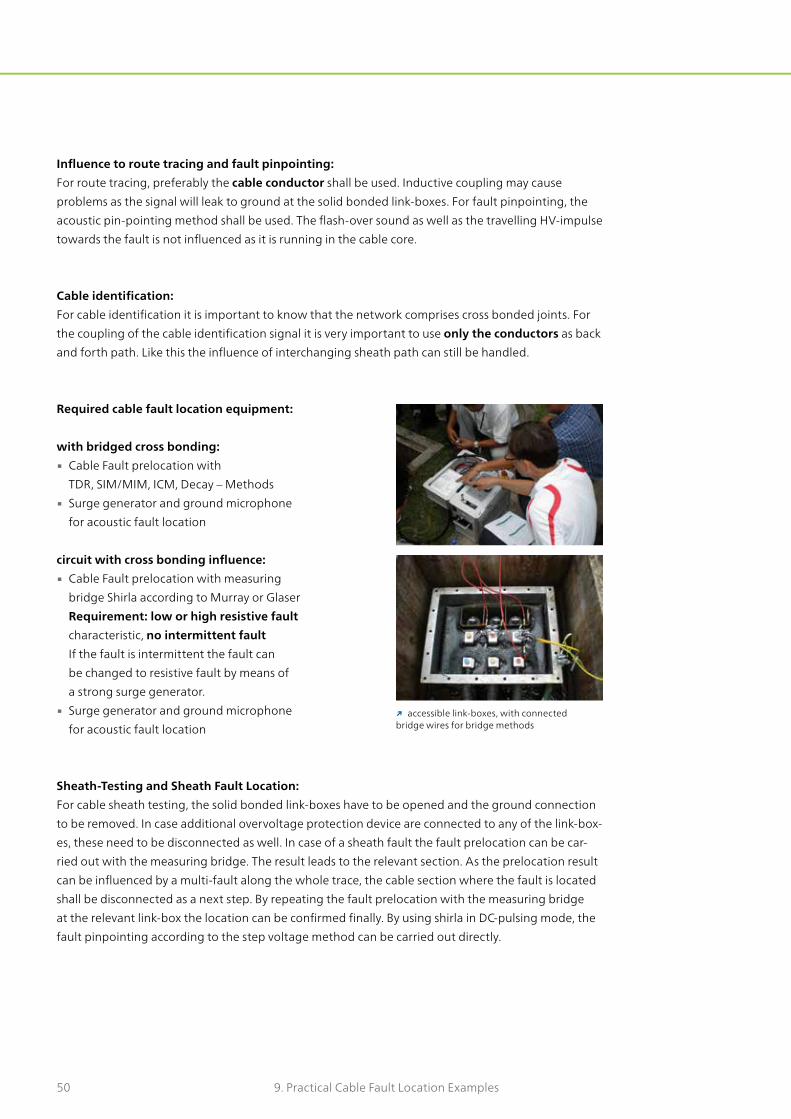
50 9. Practical Cable Fault Location Examples
Influence to route tracing and fault pinpointing: For route tracing, preferably the cable conductor shall be used. Inductive coupling may cause problems as the signal will leak to ground at the solid bonded link-boxes. For fault pinpointing, the acoustic pin-pointing method shall be used. The flash-over sound as well as the travelling HV-impulse towards the fault is not influenced as it is running in the cable core.
Cable identification: For cable identification it is important to know that the network comprises cross bonded joints. For the coupling of the cable identification signal it is very important to use only the conductors as back and forth path. Like this the influence of interchanging sheath path can still be handled.
Required cable fault location equipment:
with bridged cross bonding: ▪ Cable Fault prelocation with
TDR, SIM/MIM, ICM, Decay – Methods ▪ Surge generator and ground microphone
for acoustic fault location
circuit with cross bonding influence: ▪ Cable Fault prelocation with measuring
bridge Shirla according to Murray or Glaser Requirement: low or high resistive fault characteristic, no intermittent fault If the fault is intermittent the fault can be changed to resistive fault by means of a strong surge generator.
▪ Surge generator and ground microphone for acoustic fault location
Sheath-Testing and Sheath Fault Location: For cable sheath testing, the solid bonded link-boxes have to be opened and the ground connection to be removed. In case additional overvoltage protection device are connected to any of the link-box-es, these need to be disconnected as well. In case of a sheath fault the fault prelocation can be car-ried out with the measuring bridge. The result leads to the relevant section. As the prelocation result can be influenced by a multi-fault along the whole trace, the cable section where the fault is located shall be disconnected as a next step. By repeating the fault prelocation with the measuring bridge at the relevant link-box the location can be confirmed finally. By using shirla in DC-pulsing mode, the fault pinpointing according to the step voltage method can be carried out directly.
↗ accessible link-boxes, with connected bridge wires for bridge methods

519. Practical Cable Fault Location Examples
↗ TDR Measurement result with IRG 3000, positive reflection at 6814 m
↗ IRG 3000 / Syscompact 3000 ↗ Termination: Ang M. K. 66 kV Substation, SF 6
↗ TDR Measurement with IRG 2000, positive reflection visible
↗ Link box with open link connectors at 6814 m
9.2 Experience with TDR in Cross Bonding Arrangement
Conditions: 66kV XLPE cable Single core Total cable length 14,930 m Number of link-boxes: 42
Arrangement: 2x IJ… joint with cross-bonding 1x NJ ... solid bond joint (see Fig. on page 49)
Measuring bridge could not be applied due to induced voltage. An alternative solution was tried with IRG 3000 (400 V voltage proof).

52 9. Practical Cable Fault Location Examples
TDR in general is influenced by cross-bonding joints. The impedance at each joint is changing and causing the TDR pulse to be reflected. In general it is known that after 2-3 cross-bonding joints, the TDR pulse is strongly reflected and can hardly travel further along the cable. IRG 3000 and IRG 2000 can be used with automatic parameter setting. Upon selection of long view range in order to visualize the whole cable length on the screen, a TDR pulse with wide pulse width is selected. Accordingly the pulse has a higher energy and is supposed to travel longer distances. In cross-bonding arrangements it was recognized, that a pulse with wider pulse width suffers higher reflection at cross-bonding joints compared to pulses with narrow pulse width. In this particular case it was found, that with the setting of the ideal pulse width the TDR meas-urement was possible in order to see the cable interruption at 6814 m.
Effect of different Pulse Width:
Too wide pulse width ▪ Strong reflection at first
cross-bonding joints ▪ Reflections beyond 2-3
joints are no more clear
Ideal pulse width ▪ Slight reflection at
crossbonding joints ▪ Pulse is able to travel
through the cross-bonding
Too narrow pulse width ▪ The energy of the pulse is very
weak, only the first section of the able is reflected.
▪ The pulse is damped off.
↗ Voltage: 40 V, Pulse Width: 10,000 ns
↗ Voltage: 40 V, Pulse Width: 2,000 ns / ideal pulse width
↗ Voltage: 40 V, Pulse Width: 100 ns

539. Practical Cable Fault Location Examples
Low Pulse Voltage ▪ Reflections of close range cable
section is very clear
Medium Pulse Voltage ▪ Reflection of middle range cable
section is very clear
High Pulse Voltage ▪ Reflections in long range cable
sectionis clear
↗ Voltage: 40 V, Pulse Width: 2000 ns
↗ Voltage: 80 V, Pulse Width: 2000 ns
↗ Voltage: 160 V, Pulse Width: 2000 ns
Effect of different Pulse Voltage:
Application of higher pulse voltage effects in more signif-icant impedance change and allows seeing impedance changes over longer distances. The selection of the right setting is depending on the point of focus. If the fault is far from the connection point, higher pulse voltage is re-quired. If the fault is close to the connection point, the near cable section is shown clearer if the selected pulse voltage is lower. The success with TDR in cross-bonding arrange-ments is depending on the cross-bonding arrangement and design of the Joint - Linkbox arrangement.
The distance between the joint (e.g. under the road) and the Link box (e.g. on the road side) is relevant and influenc-ing the impedance change.
The TDR Method allows identifying: ▪ Interruptions in the sheath, e.g. open connector at any of
the link boxes ▪ low resistive faults (between core and sheath) ▪ Open circuit, common characteristic after a joint failure,
parts of the AL conductor vaporized
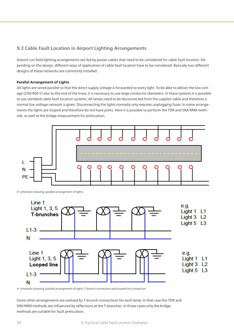
54 9. Practical Cable Fault Location Examples
9.3 Cable Fault Location in Airport Lighting Arrangements
Airport run field lighting arrangements are fed by power cables that need to be considered for cable fault location. De-pending on the design, different ways of application of cable fault location have to be considered. Basically two different designs of these networks are commonly installed.
Parallel Arrangement of LightsAll lights are wired parallel so that the direct supply voltage is forwarded to every light. To be able to deliver the low volt-age (230/400 V) also to the end of the trace, it is necessary to use large conductor diameters. In these systems it is possible to use standard cable fault location systems. All lamps need to be disconnected from the supplier cable and therefore a normal low voltage network is given. Disconnecting the lights normally only requires unplugging fuses. In some arrange-ments the lights are looped and therefore do not have joints. Here it is possible to perform the TDR and SIM/MIM meth-ods, as well as the bridge measurement for prelocation.
Some other arrangements are realized by T-brunch connections for each lamp. In that case the TDR and SIM/MIM methods are influenced by reflections at the T-branches. In those cases only the bridge methods are suitable for fault prelocation.
↗ schematic drawing, parallel arrangement of lights, T-branch connection and looped line connection
↗ schematic drawing, parallel arrangement of lights

559. Practical Cable Fault Location Examples
↗ schematic drawing, serial arrangement of lights with transformers
The required equipment therefore is consisting of the following instruments:In Networks without T-branches
▪ Low Voltage Cable Fault Location System STG 600 + IRG 2000 → For prelocation of low-, high resistive and intermittent faults
according to TDR and SIM/MIM ▪ Surge Generator STG 600 in surge mode
→ for fault pinpointing according to the acoustic fault location method in combination with the ground microphone UL / BM
In Networks with T-branches ▪ High Voltage Measuring Bridge shirla
→ For prelocation of low and high resistive faults according to Murray or Glaser bridge methods
▪ Surge Generator SSG 500 → For fault pinpointing according to the acoustic fault location method
in combination with the ground microphone UL / BM
Serial Arrangement of Lights with TransformersA way of network design that was used in earlier installations of airport lighting was comprising a high voltage cable ring. Every light is linked to the high voltage cable by means of a transformer. The primary sides of the transformers is connect-ed in line to each other. Depending on the number of transformers, the feeding voltage is set by means of an adjustable high voltage transformer.
The lights are again divided into several circuits that are arranged, as shown in the schematic diagram. For this type of network it is not necessary to use big diameters for the conductors, as the network is operated with high voltage. Fur-thermore it is more flexible and more capable for enlargement and extension. Every lamp is equiped with a separation transformer, so that every transformer causes a voltage drop defined by the each transformer primary winding. For every light the same voltage drop and the same voltage is obtained. All lights are designed to be unplugged easily at the trans-former. All primary sides of the transformer are connected in line. When performing a resistance measurement the value of measurement is including all resistances of the primary sides of all transformers connected in line. To be able to perform a fault prelocation measurement it is required disconnect all lamps to prevent any damage.

56 9. Practical Cable Fault Location Examples
For cable fault prelocation only the bridge method can be applied successfully. The cable circuit can be considered a serial circuit of line-resistances of the cable sections and winding-resistances of the transformer primary sides. Old measuring technology based on a simple measuring bridge required to work with complicated calculations to bring the resistances into relation with the actual positions. According to this calcualtion, the measured galvanometer reading could be transferred to the field.
The modern high voltage measuring bridge shirla has been designed in consideration of such an application. With this instrument it is possible to define the line charac-teristic by means of sectors.
The resistance of the first sector up to the first transformer is defined by the diameter, material and length of the cable section. The resistance of the primary winding of each transformer can be measured and recalculated out of the substituting relation of:
RP =!C ! lAV
whereby the parameters are:
RP ... Resistance of primary winding,ρC ... Copper (selectable),l ... approx. 0.2m,AV ... virtual cross section received out of calculation
AV =!C ! lRP
The operation menu of shirla enables to enter the indi-vidual sections (cable, transformer, cable,…) accordingly. The measured result is then automatically calculated based on the entered sections with their individual parameters. Already after the first measurement, the relevant section can be determinated.
For fault pinpointing the relevant cable section can be disconnected at both sides. By means of application of a surge generator the cable fault pinpointing according to the acoustic method can be applied.
The required equipment therefore is consisting of the following instruments:
▪ High voltage measuring bridge shirla → For prelocation of low and high resistive faults accord-
ing to Murray or Glaser bridge methods ▪ Surge Generator SSG 500
→ For fault pinpointing according to the acoustic fault location method in combination with the ground microphone UL / BM
↗ shirla (SHeath, Insulation test, fault Resistance and Location Analyzer)
↗ airport light connected via separa-tion transformer

579. Practical Cable Fault Location Examples
↗ vaporized core after cable fault, 132 kV XLPE
↗ exploded 132 kV joint after cable fault, 132 kV XLPE, explosion lifted soil above the faulty spot.
↗ Cable Fault in a 132 kV PILC cable
9.4 Cable Fault location in High Voltage cables e.g. 115kV
High voltage cables such as e.g. 115 kV cables, 230 kV cables or similar are mainly operated at high load. In case of a cable fault the flash over energy is very high.
XLPE Cables:In XLPE cables most often a big explosion is happening and the cable parts around the fault are burnt and/or va-porized completely. Also the other cores as well as neigh-bouring cables are very often damaged beside. Due to this reason cable fault location can be carried out easily with basic cable fault location equipment used for medium voltage cables. A fault location system based on a surge generator up to 32 kV is mostly fully sufficient to prelocate these cable faults. The comparison of TDR graphs of a healthy core in comparison with the faulty phase leads to precise cable fault prelocation graphs in low resistive fault conditions. Depending on the current load of the cable at the moment of flash over the conditions may also remain high resistive or intermittent. In general the 32 kV surge generator combined with the SIM/MIM or ICM method can cover these fault conditions. If the fault condition shows solid grounded conditions the pin pointing may not be possible by means of the acoustic fault location method as no flash over can take place at a short circuit fault. In such a case the step voltage method is the only method to perform the cable fault pin pointing in 1-core cables. In 3-core cables, which are used rarely, also the Twist Method can be used for pin pointing.
PILC Cables:High voltage PILC cables are more resistant to the flash over. In these cables the remaining fault condition may be an intermittent fault with a certain breakdown voltage possibly higher than 32 kV. To prelocate such faults the Decay method based on a HV DC or VLF instrument that is covering the breakdown volt-age is required. Basically all these available HV instruments enable to be used in burnmode. Most of the fault condi-tions can be changed by application of the burn mode over a certain time. During this fault burning the paper insula-tion is carbonizing and the break down voltage of the fault can be reduced. Finally for pin pointing a surge generator with a maximum output voltage of 32 kV can be applied. Only very seldom it is required to use a surge generator with higher output voltage.


BAUR GmbH · Raiffeisenstrasse 8 · 6832 Sulz · AustriaT +43 5522 4941-0 · F +43 5522 4941-3 · [email protected] · www.baur.eu
Other BAUR Brochures
Item No. 821-070 01/16Subject to modifications.
Other BAUR Brochures
BAUR company brochure
Cable testing and diagnostics
Cable fault locationBAUR product overview
Our brochures and manuals are also available online at: www.baur.eu/brochures
Cable test vans and systems
Insulating oil testing