application of conditional geostatistical simulation to ...hera.ugr.es/doi/15024696.pdf ·...
TRANSCRIPT

Geophys. J. Int. (1999) 139, 703–725
Application of conditional geostatistical simulation to calculate theprobability of occurrence of earthquakes belonging to a seismic series
Federico Torcal,1 Antonio M. Posadas,1,2 Mario Chica3 and Inmaculada Serrano11 Instituto Andaluz de Geofısica y Prevencion de Desastres Sısmicos, Observatorio de Cartuja, Campus Universitario de Cartuja s/n, 18071 Granada,
Spain. E-mail: [email protected]; [email protected]
2Departamento de Fısica Aplicada, Universidad de Almerıa, L a Canada de San Urbano, 04120 Almeria, Spain. E-mail: [email protected]
3Departamento de Geodinamica, Universidad de Granada, Facultad de Ciencias, Avenida de Fuentenueva s/n, 18003 Granada, Spain.
E-mail: [email protected]
Accepted 1999 July 7. Received 1999 February 25; in original form 1998 January 25
SUMMARYGeostatistics offers various techniques of estimation and simulation that have beensatisfactorily applied in solving geological problems. In this sense, conditional geostatisticalsimulation is applied to calculate the probability of occurrence of an earthquake witha lower than or equal magnitude to one determined during a seismic series. It ispossible to calculate the energy of the next most probable earthquake from a specifictime, given knowledge of the structure existing among earthquakes occurring prior toa specific moment.
Key words: Almerıa, earthquake prediction, geostatistics, statistical methods.
distribution (Journel & Huijbregts 1978). If the random1 INTRODUCTION
variable is distributed in space and/or time we say that it is aregionalized variable. These variables, due to their spatial-The methods that enable us to study seismic series from spatialtemporal character, have a random as well as a structuralas well as temporal or energetic points of view can be classifiedcomponent (Matheron 1963). At first sight, a regionalizedinto two types: deterministic and probabilistic methods. In thisvariable seems to be a contradiction. In one sense it is astudy we suggest the use of probabilistic methods, founded inrandom variable that locally does not have any relation toprobability theory, because of the lack of information aboutthe nearby variables. On the other hand, there is a structuralthe causes of the sequence of seismic events (Kagan 1992); theaspect in the regionalized variable that depends on the distancecomplexity of the cause–effect relations of the seismic seriesof separation of the variables. Both characteristics can be(De Miguel 1976; Posadas et al. 1993a,b); the fact that thedescribed, however, using a random function for which eachearthquakes are considered as non-linear, chaotic phenomenaregionalized variable is a particular realization. By incorporating(Kagan 1997; Feng et al. 1997) that are self-similar with nothe random as well as the structural aspects of a variable in ascale variability (Kagan 1997); the lack of a complete theorysimple function, the spatial variability can be accommodatedabout the occurrence of earthquakes; the complexity and theon the basis of the spatial structure shown by these variablesdifficulty in interpreting the character of the data; the multitude(Carr 1983). In this sense, a regionalized variable is a variableof variables involved in an earthquake (which implies that wethat qualifies a phenomenon that is distributed through spaceare dealing with a multidimensional process); and variousand/or in time and that presents a certain correlation structureother factors (Kagan & Jackson 1996).(Chica Olmo 1987). To date, regionalized variables have beenGeostatistics offers various methods that are important inused in geological disciplines that represent phenomena in aquantifying and solving for many geological variables. Allqualitative as well as quantitative manner; for example, thethese methods consider the value of each point as well as thelaw of a mineral, the thickness of strata, the pluviometry of aspatial and/or temporal position of each point with respect toregion, the impermeability of the land and the resistivity ofthe others. This aspect achieves results that approximate thethe ground.real values better than those reached with other methods.
On the other hand, one of the most characteristic aspects ofseismic activity is that it usually occurs in the form of a seismicseries. A seismic series is a set of earthquakes occurring in a2 SOME IMPORTANT CONCEPTSgiven period of time in a given area. Seismic series are common
Geostatistics has its basis in Matheron’s (1965) Theory of in some regions. Gutenberg & Richter (1954) defined seismicityRegionalized variables. A random variable is one that has a as an activity of fluctuating fracturation associated with
earthquakes.variety of values in accordance with a particular probability
703© 1999 RAS

704 F. T orcal et al.
Earthquakes of a seismic series have a similar spatial and structure of a regionalized variable is to relate the changes
between the variables to the distance that separates them. Iftemporal genesis, so form sets of inherently correlated data. Aset of observed earthquakes can be considered as an estimator the average difference between the variables increases as the
separation distance increases, there is a spatial structure andof the properties of the totality of the population of past and
future events within a defined region (Udıas & Rice 1975). the variables are regionalized. If, on the other hand, the averagedifference between the variables changes erratically, irrespectiveThe estimation of the scaling properties of several geophysical
systems can be significantly influenced by the use of sets of of the distance of separation, the variable is random and
there is not a spatial structure. It is thus possible to identifydata that are limited in quantity of data available as well asin the size of the volumes of study and measurement errors analytically the spatial behaviour of a random variable (Carr
1983).(Eneva 1996). Thus, Eneva (1996) concludes that the bias of the
estimations of the correlated dimensions from a set of limited Taking into account the concept of statistical variance, andconsidering that the expectation of a random function at pointdata can readily be evaluated, making it unnecessary to work
with ever-increasing sets of data, and thus small sets of data x is the mean m (x), then the variance is an expectation and is
(Journel & Huijbregts 1978)can be effectively used to observe temporal variations in thescale properties that may be associated with the occurrence of
Var{Mag(x)}=E{[Mag(x)−m(x)]2} . (1)larger events. From a geostatistical point of view, the seismic
series make up a set of data appropriate for the study of For two regionalized variables Mag(x1 ) and Mag (x2 ), whichmethods that determine parameters or properties that may be have variances in x1 and x2 , a covariance that relates theseof interest. variables can be expressed (Journel & Huijbregts 1978) as
Earthquakes of a seismic series are considered as stochasticC(Mag(x
1), Mag(x
2))=E{[Mag(x
1)−m(x
1)]
mathematical variables, belonging to a continuous space–time–energy medium with dimension 5 (Q
i, l
i, h
i, ti, M
i), where Q
i ×[Mag(x2)−m(x2 )]} . (2)
is latitude, li
longitude, hidepth, t
itime and M
imagnitude
The intrinsic geostatistical hypothesis only assumes the(Udıas & Rice 1975). The earthquakes of a seismic seriesstationarity of the second order of the increases, and so thereflect a clear activity in one area and for a delimited time.data can perfectly well have a derivative. This aspect is veryThis seismic activity is the product of the creation and/orimportant because the majority of the phenomena analysed inmovement of a fault or a system of faults. The geographicalEarth Sciences usually have derivatives/tendencies (Herzfeldcoordinates of the earthquakes analysed are considered to be1992). Owing to the fact that the intrinsic hypothesis m (x1 )=included within the system of coordinates that the seismicm (x2 ) holds, the variance of the incremental difference betweenseries covers; that is, the system of faults that produces thethe variables Mag (x1 ) and Mag(x2 ) can be expressed as follows:seismic activity. So, in this paper we consider only the temporal
and energy coordinates. The temporal coordinate will be 2c[Mag(x1), Mag(x
2]=Var{Mag(x
1), Mag(x
2)}
understood as the order of sequence within the seismic series=E{[Mag(x
1)−Mag(x
2)]2} . (3)and not as absolute time.
If the activity develops without abrupt changes during the If the points x1 and x2 are separated by a distance h, thenfault process that produces the earthquake, or if no other fault x1=x, x2=x+h, andsystem develops, it is possible to know the structure that exists
2c(h)=E{[Mag(x)−Mag(x+h)]2} (4)between the earthquakes. This is shown using the variogramfunction; if there were to be a change in the correlation andstructure of the data it would be reflected in a change in the
c(h)=(1/2)E{[Mag(x)−Mag(x+h)]2} . (5)kind and parameters that define this function.The data on the occurrence of earthquakes and the resulting Eq. (4) defines the analytical equation of the variogram (or
release of energy occurring up to a given moment provide variogram function), and eq. (5) defines the semi-variogram,information about the structure and the relation that exist although it is very common to call the semi-variogram theamong these earthquakes. This is precisely the moment to take variogram too. These equations describe the structural aspectadvantage of this information, which allows us to know what of a regionalized variable, and the function c measures theis most likely to happen after a given time. spatial continuity, or, in other words, the spatial correlation.
In this case, c(h) represents half of the average of the squares
of the differences between the magnitudes of the earthquakes3 VARIOGRAM CONCEPTseparated by a step or distance h. Since this methodology
From a geostatistical point of view, the sequence of magnitudes originated in the solution of mining problems, some of theof the earthquakes of a seismic series can be considered as a original terms are retained, such as the case of the step h orregionalized variable. This variable is interpreted as a function distance. In this way, it is deduced that c(h) is a vectorialmag(x) that provides the magnitude mag of an earthquake x function depending on the modulus and the angle of the vectorwithin the sequence of a seismic series. The regionalized of distance h. Considering the sequence of the magnitudes ofvariable mag(x) behaves like a random variable, and an a seismic series, the vector distance h is linear (angle=0°) andearthquake can be considered as a particular realization of the its modulus is a function of the order of the sequence.random function Mag (x), made up of a set of random variables The statistical inference of the direct variogram is obtained[mag(x1 ), mag (x2 ), … , mag(x
n)], a sequence of earthquakes from the estimator c*(h) of the variogram c(h) of eq. (5):
within the seismic series. The transitional behaviour (betweena deterministic and random state) is typical of a regionalized
c*(h)=1
2Np(h)∑Np(h)
i=1[Mag(x)−Mag(x+h)]2 , (6)
variable (Herzfeld 1992). One way of examining the spatial
© 1999 RAS, GJI 139, 703–725

Earthquake probabilities in a seismic series 705
where Np(h) is the number of pairs of magnitudes of the4.1 Basic statistical treatment and experimental
earthquakes at a distance h, and this equation represents halfvariographic analysis
of the average squared increases between the earthquakemagnitudes separated by a distance h.
4.1.1 Basic statistical treatment
As a first step, the quality of the data is proved, and the basic4 THE CONDITIONAL GEOSTATISTICAL statistical calcultations from which the statistics or measure-SIMULATION METHOD FOR THE ments are obtained are performed. These are the numericalENERGETIC SIMULATION OF SEISMIC values that enable us to characterize and compare the statisticalSERIES distributions. They can be of several types, as follows.
As in almost all of the fundamental concepts of geostatistics,Measurements of centralization. These measurements indicate
the first steps of the geostatistical simulation method werea value around which the distribution values are distributed.
given by Matheron, who proposed and implemented thisThey are generically known as means, and have the following
method in the form of the T urning Bands Method. Later, theforms.
theoretical bases were affirmed and supported (Guibal 1972;
Journel 1974a,b; Chiles 1977; Journel & Huijbregts 1978; T he arithmetic mean or mean, m.Alfaro 1979) and the first applications appeared (Deraisme T he median, M, is the value that divides the population into1978a,b). two equal parts. It is the quartile of 50 per cent.
The development of this methodology originally came from T he lower quartile, Q1 , is the value with 25 per cent of thethe mining industry, to solve the problems found in design population below it and the remaining 75 per cent above it.and mining planning in which the values estimated turned out T he upper quartile, Q3 , is the value with 75 per cent of theto be ‘smoothed’ with respect to the real values, not reflecting population below it and the remaining 25 per cent above it.the degree of variability and detail present in the values of the T he mode, Mo, is the value of the greatest absolute frequencymining variables (Armstrong & Dowd 1994). of a distribution.
From the 1980s onwards, many applications appeared, almostMeasurements of dispersion. These measurements indicateall of which were dedicated to geological mining (Dumay 1981;
the variability of dispersion of the values of a distribution.Chica Olmo 1982a,b; Deraisme et al. 1982; Chica Olmo et al.1983; Chica Olmo & Laille 1984; Deraisme et al. 1985; Chica T he variance, s2, is the average of the squares of theOlmo 1987; Schafnester & Burger 1988; Pardo Iguzquiza & deviations with respect to the mean.Chica Olmo 1989). T he standard deviation, s, is the square root of the variance
In the 1990s many theoretical aspects have been developed, and represents the margin of the variation or the error ofincluding new more efficient algorithms such as applications estimation in which the data analysed are included. It has therelevant to multiple fields, analysis of basins, treatment of same units as the variable under consideration.images, modelling of karstic media, simulations of geological T he range, R, of a distribution is the difference between thelithofacies, etc. (Armstrong & Dowd 1994). This development extreme maximum and minimum values.has been aided by the widespread use of computers, making it T he coeYcient of variation, CV , is the quotient of thepossible to deal with the numerous calculations required. standard deviation and the mean. It enables us to compare
The values of the models obtained using geostatistical simu- distributions that have different units. There is a direct relationlation agree with the experimental information and reproduce between the value of this parameter and the dispersion of thethe observed variability. distribution.
We have proved that the following functions of the real The interquartile range, IR, is the difference between the uppervalues mag (x) of a random function Mag (x) and the values quartile and the lower quartile and it indicates the range betweenobtained by conditional simulation magCS(x) coincide: which 50 per cent of the central values of the population are
distributed.the averages, E{magCS (x)}=E{mag(x)} , (7)
Distribution moments. These can be central or with respectthe variances, s2CS=s2 , (8)to the origin.
the variograms, cCS (h)=c(h) , (9)T he central moment of order r, M
r, is the average of the
and the histograms, F[magCS (x)]=F[mag(x)] . (10) deviation with respect to the mean taken to order r.
Moreover, a conditioning of the simulated model is imposed Asymmetry or skewness measurements. These provide anon the experimental values; that is, at a point or experimental idea of the asymmetry of the distribution. A distribution istime x, the simulated and the experimental values coincide: symmetric when the frequencies corresponding to equidistant
values with respect to a central value are equal. In the idealmagCS (x)=mag(x) . (11)symmetry condition, the values of the mean, median and mode
coincide. A distribution has a bias to the right or is positiveThe fact that the variograms of the simulated values andthe real values coincide implies that both sets of values have (+) if the frequencies descend more slowly on the right of the
histogram. In this case, the mean is greater than the mode. Athe same spatial and/or temporal variability.
The steps for obtaining numerical model of simulation from distribution has its bias to the left or is negative (−) if thefrequencies descend more slowly on the left of the histogram.the experimental data (Pardo Iguzquiza et al. 1992) are given
below. In this case, the mean is less than the mode.
© 1999 RAS, GJI 139, 703–725
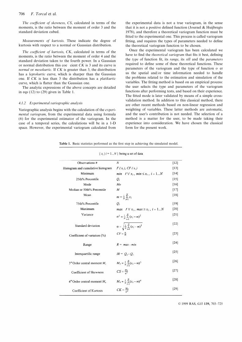
706 F. T orcal et al.
T he coeYcient of skewness, CS, calculated in terms of the the experimental data is not a true variogram, in the sense
moments, is the ratio between the moment of order 3 and the that it is not a positive defined function (Journel & Huijbregtsstandard deviation cubed. 1978), and therefore a theoretical variogram function must be
fitted to the experimental one. This process is called variogramMeasurements of kurtosis. These indicate the degree of fitting, and requires the types of parameters needed to define
kurtosis with respect to a normal or Gaussian distribution. the theoretical variogram function to be chosen.
Once the experimental variogram has been calculated weT he coeYcient of kurtosis, CK, calculated in terms of thehave to find the theoretical variogram that fits it best, definingmoments, is the ratio between the moment of order 4 and thethe type of function fit, its range, its sill and the parametersstandard deviation taken to the fourth power. In a Gaussianrequired to define some of these theoretical functions. Theseor normal distribution this coefficient CK is 3 and its curve isparameters of the variogram and the type of function offernormal or mesokurtic. If CK is greater than 3, the distributionus the spatial and/or time information needed to handlehas a leptokurtic curve, which is sharper than the Gaussianthe problems related to the estimation and simulation of theone. If CK is less than 3 the distribution has a platikurticvariables. The fitting method is based on an empirical process:curve, which is flatter than the Gaussian one.the user selects the type and parameters of the variogramThe analytic expressions of the above concepts are detailedfunctions after performing tests, and based on their experience.in eqs (12) to (29) given in Table 1.The fitted mode is later validated by means of a simple cross-
validation method. In addition to this classical method, there4.1.2 Experimental variographic analysis are other recent methods based on non-linear regression and
weighting of variables. These latter methods are automatic,Variographic analysis begins with the calculation of the experi-and the user’s contribution is not needed. The selection of amental variogram, from the experimental data using formulamethod is a matter for the user, to be made taking their(6) for the experimental estimator of the variogram. In theexperience into consideration. We have chosen the classicalcase of a temporal series, the calculations will be in a 1-D
space. However, the experimental variogram calculated from form for the present work.
Table 1. Basic statistics performed as the first step in achieving the simulated model.
© 1999 RAS, GJI 139, 703–725

Earthquake probabilities in a seismic series 707
Variographic analysis is very important because it enables In order to calculate the Gaussian values, we use the
cumulative histogram without grouping the data in classes,us to define the structure of the data, and the degree ofcorrelation. Note that the variogram function indicates the but considering the data individually. They are normally put
in increasing order and the value of the following distributionvariability that exists among the data in the set considered. In
the case when the variogram is stationary, that is it reaches a probability function is assigned to each experimental value z:limiting value in its growth (sill ) that represents the maximumvariability or minimum correlation among the data, the relation F(mag(x))=P[Mag(x)≤mag(x)]=
n
N+1, (34)
between the variogram function and the covariance functionis given by the expression where F(mag (x) ) is the distribution function of experimental
probability for the experimental value mag(x), n is the positionc(h)=s2−C(h) . (30)
of the datum mag (x) in the sequence of ordered values, and Nis the total number of experimental values.From this we can deduce that the variogram and the covariance
As can be seen, the Gaussian values obtained are independentfunctions are symmetrical if the phenomenon with which weof the numerical value of the experimental values. If we findare dealing is stationary.several values repeated then we assign the same GaussianFrom expression (30) we also define the correlogram, r(h),probability to all of them—that calculated for the element ofand the relative variogram, cr (h), which enable us to comparegreatest order.series of different data. Thus, if we normalize the previous
Next, the Gaussian values are calculated from the inverseexpression with respect to the variance s2 we haveGaussian function using the rational approximation given byAbramowitz & Stegun (1964). Ifc(h)
s2=1−
C(h)
s2, (31)
F(mag(xi) )≤5[ y
i=G−1[F(mag(x
i))] , (35)
from whichbut if
cr (h)=1−r(h) . (32)F(mag(x
i) )>0.5[F(mag(x
i))=1−F(mag(x
i)) . (36)
As Pardo-Iguzquiza et al. (1992) indicate, this entire analysis If we defineof structural character can be performed using three momentsof the conditional geostatistical simulation process: first, on
t=SlnC 1
F(mag(xi))2D , (37)the experimental data to characterize its spatial variability;
second, on the normalized values obtained when the experi-thenmental values have been transformed by the non-conditional
simulation; and third on the values obtained as a result ofyi=G−1[F(mag(x
i) )]=t−
a0+a
1t+a
2t2
1+b0+b
1t+b
2t2+b
3t3
. (38)the conditional simulation in order to test the goodness of theresults obtained.
The constant values are
a0=2.515517; a
1=0.802853; a
2=0.010328;4.2 Gaussian anamorphosis and variographic analysis on
the Gaussian data b1=1.432788; b
2=0.189269; b
3=0.001308;
The methods of non-conditional geostatistical simulation i=1 … N .generate a set of simulated values with a distribution function
Once the correspondence between the experimental valuesof the probability of centred and reduced Gaussian probabilitymag (x
i) and their respective Gaussian values y
ihas beenN(0, 1). In order to transform these data into real units, by
obtained, we can restore any Gaussian value to real unitsconserving the histogram of the regionalized variable, we useusing a linear interpolation between the immediate superiorthe so-called anamorphosis function (Journel 1974b; Marechaland inferior values in such a way that if1975, 1978; Journel & Huijbregts 1978; Chica Olmo 1987):
yµ[yi, yi+1][mag(x)µ[mag(x
i), mag(x
i+1 )] (39)G(y) cfbbew(y)
w−1 (mag(x) )F(mag(x)) , (33)
and then
where G ( y) is the Gaussian distribution function N(0, 1),mag(x)=mag(x
i)+
mag(xi+1)−mag(x
i)
yi+1−y
i(y−y
i) . (40)
F(mag (x) ) is the experimental distribution function, w( y) is the
direct anamorphosis function, and w−1 (mag (x) ) is the inverseThis transformation is known as direct Gaussian anamorphosis.
anamorphosis function.Outside the range of experimental values, the anamorphosis
The distribution function of the probability of the experi-function is not known and so it is necessary to model it
mental data for the case of geological and geophysical variablestheoretically. To do this we use the method called Gaussian
is unknown in the majority of the cases. The experimentalModelization of the Distribution Tails of Pardo-Iguzquiza
histogram is therefore usually considered to be sufficiently(1989, 1991). In this method we consider that, when the
representative (Journel 1974b). This histogram can reflect anydistribution probability function of a random function Mag (x)
model of the distribution probability function, but the mostis Gaussian, the anamorphosis function is a straight line with
frequently used algorithms in the non-conditional geostatisticala slope equal to the standard deviation and whose intersection
simulation produce simulated values with a distributionwith the axis is equal to the mean; that is,
function of Gaussian probability, as a result of the Theoremof the Central Limit (Marechal 1975). mag(x)=sy+m . (41)
© 1999 RAS, GJI 139, 703–725

708 F. T orcal et al.
Assuming that the probability determined by the distribution simulation that the method proposed by Shinozuka & Jan
(1972) uses. This is a technique in the frequency domain, wherefunction of Gaussian probability below and above the values−4 and 4 is sufficiently small, the spectral density function is determined by a Fourier
transform of the covariance function.P(y<−4)=P(y>4)=3.20×10⁻⁵ , (42)
In the case of stationary random functions, this spectraldensity function represents the distribution of the variance inthe following can be taken as extreme values:terms of the frequency. The generator of the simulated values
mag(x)min=−4s+m , (43)is expressed as follows:
mag(x)max=−4s+m . (44)
mags (x)=2 ∑N
i=1[S(v)Dv]1/2 cos(v
ix+w
i) , (45)The construction of the end part of the tail is carried out for
the tracing of the left part by joining the pointswhere mags (x) is the value of the simulated magnitude at point
(−4, mag(x)min) and (y1, mag(x)
1) , x, S(v) is the spectral density function, v is the frequency, i is
the order of the harmonic, N is the number of harmonics used,where −4 is the minimum theoretical Gaussian value,Dv is the discretized frequency, v
iis the frequency to which amag(x)min is the minimum theoretical value, y1 is the minimum
small random frequency is added in order to avoid periodicities,Gaussian value and mag(x)1 is the minimum experimentaland w
iare independent random angles uniformly distributedvalue. In order to trace the right part, the following points are
between 0 and 2p.joined:The most common formulas for S(v) for the most widely
(4, mag(x)max ) and (yn, mag(x)
n) , used models in geostatistics (Pardo-Iguzquiza et al. 1992) are
detailed in eqs (46)–(51) given in Table 2.where 4 is the maximum Gaussian theoretical value, mag(x)maxis the maximum theoretical value, y
nis the maximum Gaussian
value and mag (x)n
is the maximum experimental value. With4.4 Conditioning of the simulation of the experimental
this method we can avoid artificial densities in the tails.values
The number of possible simulations of a random function4.3 Non-conditional simulation
Mag (x) that fulfil the condition of being isomorphic to theexperimental realization, meaning that they have the sameWithin the theory of stochastic processes we can find a number
of probabilistic methods for 1-D simulations of processes that mean and variance values and the same variogram functions,is infinite.have a covariance function C(h), which is the same as a
determined variogram function c(h). These methods can be The conditioning process of the simulation enables us to
choose from all the possible realizations of the simulationdivided into two fundamental types: methods in the domainof space or time; and methods in the frequency domain, also those that incorporate the experimental data points. To do this,
starting from non-conditional simulation, a series of operationsknown as spectral methods.
Here we have used the program 1 (Pardo-Iguzquiza to make the simulated values coincide with the experimentalvalues is carried out. This is achieved using a technique calledet al. 1992) to carry out the calculations of the conditional
Table 2. Analytic expressions for S(v) for the most widely used models (modified from
Pardo-Iguzquiza et al. 1992).
© 1999 RAS, GJI 139, 703–725

Earthquake probabilities in a seismic series 709
kriging (Matheron 1970; Journel & Huijbregts 1978): rest of the earthquakes were of lower magnitudes. Fig. 2(a) shows
the sequential evolution of the magnitudes of the seismic series:ycs (x)=ys (x)+[y*k (x)−y*sk (x)] , (52)
the order in the sequence of the series for each earthquake isshown on the x-axis and the magnitude corresponding to each
ycs (x)=ys (x)+ ∑N
i=1li[y(x
i)−ys (xi )] , (53)
event is shown on the y-axis. Fig. 2(b) shows the temporalevolution of the magnitudes, with the time of occurrence on
where ycs (x) is the conditionally simulated Gaussian datum, the x-axis. The time is expressed in days, taking as the originys (x) is the non-conditionally simulated Gaussian datum, y(x) 00 : 00 hr on the day when the first earthquake of the seriesis the normalized experimental datum, y*k (x) is the value esti- occurred. This graph clearly shows the short time that there ismated by kriging from the datum y(x), y*sk (x) is the value between the first few earthquakes, and especially the differenceestimated by kriging from the datum ys (x), l
iare the measured of scarcely 4 hr between the first earthquake of the series of
weights of the kriging system, and N is the number of nearby magnitude 5.0 and the first earthquake of magnitude 4.0,points to be considered in the kriging. and in addition some earthquakes and microearthquakes in
between them. We can also see that, after 17 days, the frequencyof earthquakes becomes lower and decreases progressively.4.5 Restoration of the experimental histogram using80 days after the occurrence of the first earthquake, the seriesdirect Gaussian anamorphosisends with an earthquake of magnitude 2.8.
Once we have the conditioned Gaussian values, it is possible Some of the earthquakes of this series were felt by theto calculate the real units to which the Gaussian values population, with intensities that varied between II and VIIcorrespond using the process of calculation of the direct degrees on the MSK scale. The stronger earthquakes were feltGaussian anamorphosis, previously mentioned in Section 4.2. in towns situated some hundreds of kilometres from the
epicentre, and in the nearest towns, such as Adra, Balanegra,
Balerma and Berja, major damage was caused to the buildings.4.6 Numerical validation of the simulated model
Finally we prove that the simulated data satisfy the geo-5.2 Estimation of the error in the measurement of thestatistical hypotheses that are considered in their calculation.magnitudeTo do this, the fundamental statistical data are studied, the
histogram and variogram as well as the experimental and The magnitudes of these earthquakes have been calculatedthe simulated values, and then they are compared. from the duration of the seismic recordings established by
We also prove that, since we consider a data series of real De Miguel et al. (1988):magnitudes but randomly ordered, when we calculate the
Md= (1.67±0.11) log t− (0.43±0.19) . (54)experimental variogram we obtain a random variogram, which
is a reflection of the fact that the existing structure among the These authors also found that, because the epicentral distancereal data is lost. term had an influence of the order of 10−4 times the epicentre–
station distance, for distances less than 1000 km (area coveredby the RSA) this influence was in all cases less than 0.1 degrees
5 APPLICATION OF THE METHOD TOof magnitude and the corresponding term was eliminated. The
THE BERJA SEISMIC SERIES ( ALMERIA,epicentre–station distances are in this case of the order of
SOUTH EAST SPAIN ) 1993 DECEMBER– 199470–120 km.
MARCHAssuming an error in the reading of the analogue recordings
of 0.5 s, equivalent to 1 mm of distance (120 mm=1 min), the5.1 Description of the seismic series
estimation errors of each magnitude are summarized in Fig. 3.
The curve that gives the standard error of the estimation ofAll the data of the seismic series that are presented come fromthe Red Sısmica de Andalucıa (RSA, Andalusian Seismic each magnitude is the central curve. The upper and lower curves
show the errors of the maximum and minimum estimation,Network; Alguacil 1986; Alguacil et al. 1990) of the Instituto
Andaluz de Geofisica y Prevencion de Desastres Sısmicos respectively.In this study, however, the error that can be obtained when(IAGPDS, Andalusian Institute of Geophysics and Prevention
of Seismic Disasters, Granada, Spain). estimating the absolute values is not as important as the fact
that the data have a certain homogeneity; that is, they haveThe Berja (Almerıa, Spain) seismic series took place in anarea in the southeast of the Iberian Peninsula (Fig. 1a) that all been measured or calculated in the same way.
has a high level of seismicity, between 1994 December 23 and1994 March 12. The locations of the epicentres classified
5.3 Calculation of the probability of the magnitude ofaccording to magnitudes can be seen in Fig. 1(b). The locations
the next earthquake from data of previous earthquakes,of the most important towns are also included.
using conditional geostatistical simulationThe most significant data of the earthquakes in this seismic
series are given in Table 3. For each earthquake in order, the Before we present the simulations, it is important to note that
each one of the probability curves calculated is the result ofdate, time and magnitude according to the Richter scale arespecified. In the date we include the year, month and day, and 100 simulations. Each one of the simulations was carried out
using data from the earthquakes prior to each one considered,in the time, the hour and the minute.
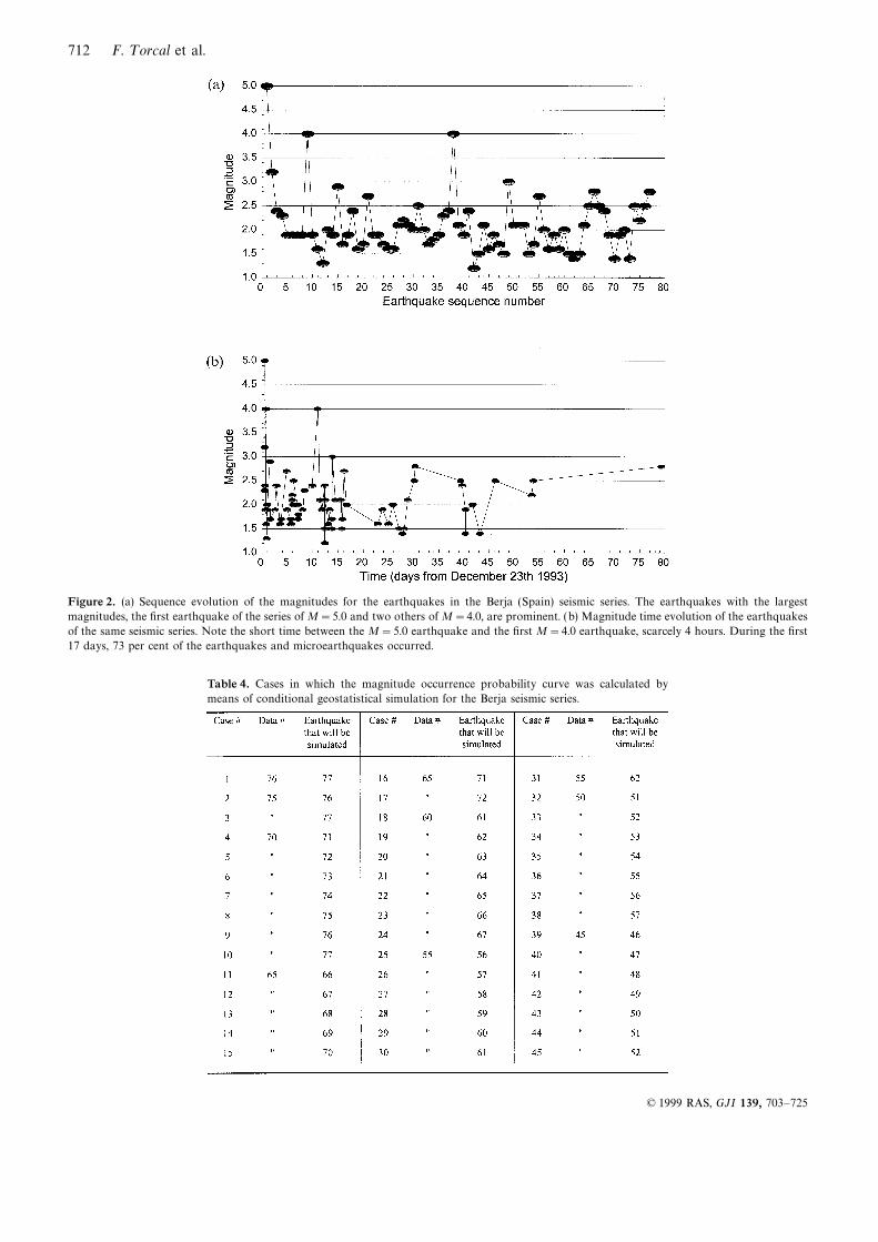
The seismic series began with the earthquake of greatest and never using data of the earthquake to be simulated or ofposterior earthquakes. This method, then, can be applied tomagnitude, 5.0 on the Richter scale; after this there were several
aftershocks, two of which reached 4.0 on the same scale. The real seismic series as they are occurring when we know some
© 1999 RAS, GJI 139, 703–725

710 F. T orcal et al.
Figure 1. (a) Map of the area where the Berja (Almerıa, Spain) seismic series, 1993 December–1994 March, took place. (b) Map of the epicentres
of the earthquakes (enlargement of the box in part a).
earthquakes that have already occurred. The number of earth- probability curve of the occurrence of an earthquake of a given
magnitude. The results that are included are therefore thequakes that have to be known for this method to be applieddepends on the seismic series, and is determined by the moment product of 4500 simulations.from which we know their structure, using the data from the
earthquakes that have already occurred to calculate the vario-5.3.1 Basic statistical treatment and experimental variographic
gram function. This aspect will be discussed with real data later.analysis
45 cases have been considered for the study of this seismic
series and are summarized in Table 4. In each case (the entry The statistical treatment of the data is carried out in each caseas detailed in Section 4.1. The results obtained are shown ingiven on the left of each column) we assume that we know the
earthquakes that occurred up to a given time (central entry Figs 4(a) and (b). We observe a tendency to a slight reduction
in the values of the variance, the standard deviation, thein each column). From this time, earthquakes of the seriesindicated will be simulated (entry on the right of each column). variation coefficient and the central moments of the third and
fourth order as the quantity of data increases.100 simulations are carried out for the calculation of the
© 1999 RAS, GJI 139, 703–725

Earthquake probabilities in a seismic series 711
Table 3. Data of earthquakes in the Berja seismic series.
These statistical values indicate that we are dealing with data (52 per cent of the total ) (Figs 5a and b), the first 58 data(75 per cent of the total ) (Figs 5c and d) and for the completedistributions that clearly have a bias to the right (the coefficient
of skewness is greater than 0) and that are leptokurtic (the series, 77 data (Figs 5e and f ). Each one of the histograms ofthis distribution is considered representative of the distributioncoefficient of kurtosis is greater than 3); that is, they have a
greater kurtic value than the normal distribution. We can say, probability function of the same distribution. From the analysis
of the histograms it can be seen that there is an absence ofthen, that there is a relative lack of low-magnitude earthquakesand microearthquakes. This fact could be either because of the earthquakes of magnitudes 2.6 and 3.1, and of magnitudes
between 3.3 and 3.9 and between 4.1 and 4.9, both extremesreal lack of these events or because of the detection level of
the seismic stations. In this case, the first reason seems more inclusive. In these distributions we also observe that the valueof the mode (magnitude 1.9) coincides with the median valueprobable because the RSA has stations very close to the area
of interest and it is a network dedicated to the detection of around which the remainder of the values of the magnitude of
this seismic series are distributed.microearthquakes (those of magnitude lower than 3.0).In order to complete the statistical study, the histograms as The next step is to carry out the variographic analysis. Since
we had data from earthquakes that had already occurred, wewell as the cumulative histograms are shown for the first 40
© 1999 RAS, GJI 139, 703–725
712 F. T orcal et al.
Figure 2. (a) Sequence evolution of the magnitudes for the earthquakes in the Berja (Spain) seismic series. The earthquakes with the largest
magnitudes, the first earthquake of the series of M=5.0 and two others of M=4.0, are prominent. (b) Magnitude time evolution of the earthquakes
of the same seismic series. Note the short time between the M=5.0 earthquake and the first M=4.0 earthquake, scarcely 4 hours. During the first
17 days, 73 per cent of the earthquakes and microearthquakes occurred.
Table 4. Cases in which the magnitude occurrence probability curve was calculated by
means of conditional geostatistical simulation for the Berja seismic series.
© 1999 RAS, GJI 139, 703–725

Earthquake probabilities in a seismic series 713
that the value of the sill indicates the moment from which all
correlation among the data is lost and the maximum variability
is obtained. The range indicates that there is some structural
relation between the 29 (for the first case) earthquakes adjacent
(according to their sequential order) and one given earth-
quake; that is, in this seismic series in the genesis of an
earthquake, up to 29 previous earthquakes can have some sort
of influence on it, or one earthquake can have some sort of
influence on the next 29 earthquakes.
The fact that there is an experimental variogram to which
a theoretical variogram function can be fitted, as well as the
fact that the theoretical variogram that best fits is spherical,
which is a function of a high degree of continuity, show that
among these data there is some degree of structure. Although
there is also some degree of randomness, this is not absolute.
In this case we clearly appreciate the double character, randomFigure 3. Estimation errors of magnitudes of the seismic series,up to a certain degree yet structural, of this regionalizedassuming a possible error in the reading of the analogue recordings ofvariable.0.5 s, equivalent to 1 mm of distance (120 mm=1 min). The central
curve is that of the standard error, and the upper and lower curves When we analyse the experimental variograms and theare for the upper and lower limits of the error, respectively (De Miguel theoretical ones fitted for each of the cases considered, 77et al. 1988). (Fig. 6a), 76 (Fig. 6b), 75 (Fig. 6c), 70 (Fig. 6d), 65 (Fig. 6e),
60 (Fig. 6f ), 55 (Fig. 6g), 50 (Fig. 6h), 45 (Fig. 6i) and 40 data
(Fig. 6j), in a sequential way, we observe the degradationcarried out the analysis for a number of cases. From thethat the experimental variogram suffers as we consider lowercomplete series, we gradually omit data until we reach a pointnumbers of data. The definition of the sill value, which isat which it is not possible to determine with certainty aclearly seen in the first cases, is not clear in the last ones. Intheoretical variogram that fits the experimental variogram.the cases with fewer data, we can also see that the values ofThe results obtained (Englund & Sparks 1991) are given inthe points of the experimental variogram for values of step hTable 5. In these cases, the step or distance h indicates thegreater than 20 are quite erratic (the lines that appear in thenumber of earthquakes next to a given earthquake, becausegraph are indicative of points that exceed the scale of the figure),the variogram has been calculated with respect to the sequencedue to the low number of pairs that can be established toof the order of the earthquakes. In all cases, the variogram thatdefine it. It is also important to note that the range increasesfits best is spherical (Sph, in the 4th column of Table 5) withas the number of data decreases, in such a way that, in thea sill value determined by the variance (e.g. 0.383 for the firstcase where 40 data of the seismic series are considered, thiscase of Table 5) and with the range indicated in brackets (e.g.value practically coincides with the range of the theoretical(29) for the first case in Table 5), or in the usual geostatistical
notation, sill Type (range), 0.383 Sph (29). We should remember variogram. So, as the number of data decreases we can see that:
Table 5. Results from variographic analysis performed for the sequential evolution of the
Berja seismic series magnitude.
Legend:
P. K. S. (Correlation %): Points in kriging during simulation. No of adjacent points that
will be taken into account during kriging in Conditional Geostatistical Simulation. The
number in brackets shows the minimum correlation rate that exists between points spaced
out. This correlation rate will be the minimum degree of certainty for each probability
curve calculated.
© 1999 RAS, GJI 139, 703–725

714 F. T orcal et al.
Figure 4. Variations of the basic statistical parameters calculated for the sets of magnitudes of the earthquakes belonging to the Berja (Almerıa, Spain)
seismic series, 1993 December–1994 March. The values for each case, considering 40, 45, 50, 55 data, and from 58 data (75 per cent of the total )
to 77 data (complete series), are shown.
(1) The number of pairs that can be established decreases from the model that is defined until the quantity of dataincreases if we only had knowledge of the first 40–45 data. Forand so the certainty with which the variogram is calculatedthis reason, we consider that we need at least 45 data to bealso decreases.able to define a theoretical variogram without having to know(2) The sill values (defined by the variance) increase.later data, and around 50–55 to be able to fit a more viable(3) The range values of the variograms increase, in such atheoretical variogram. The variograms of the intermediateway that the last case practically coincides with the quantitycases that appear in Table 5 are models that have the varianceof data and the range of the theoretical variogram. This factvalue as the sill for the data considered. The type of variogramimplies that the variogram model that can be fitted is undefinedis spherical for this seismic series and the range value issince we only have the part of the experimental variogrambetween the range values of the previous and later variograms.previous to that delimited by the sill value.
The correlograms calculated from the theoretical variogramIf we were studying this seismic series in real time, it would fitted to the relative variogram for different numbers of data
are shown in Figs 7(a) to ( j), respectively. In every case, thenot be possible to fit a theoretical variogram with certainty
© 1999 RAS, GJI 139, 703–725

Earthquake probabilities in a seismic series 715
(a) (b)
(e) (f )
(c) (d)
Figure 5. Histograms and cumulative histograms for magnitudes of the earthquakes of the Berja seismic series. The cases considering the first
40 data, 52 per cent of the total (a and b), 58 data, 75 per cent of the total (c and d) and 77 data the complete series (e and f ).
theoretical variogram fitted to the relative variogram is the up to two previous earthquakes, the degree of certainty variesbetween 85 and 88 per cent; if there are three then it is betweensame model as that fitted to the experimental variogram,
taking into account that the sill value is equal to 1. When we 76 and 81 per cent. Another interpretation of the information
that the correlogram offers is that it determines in the same wayanalyse the relative variograms and correlograms for the casescorresponding to 77, 76 and 75 data we observe that they are the degree of certainty that we will have when we simulate the
magnitudes for one, two and three, etc., earthquakes posteriorvirtually identical. Slight differences appear as the number of
data decreases, and the degree of correlation increases very to the one determined. In this way, in this seismic series, thesimulation of the magnitude of an earthquake following a givenslightly for a given distance as we have fewer data. This is due
to the fact that fewer factors intervene in the calculation as earthquake will be possible with a degree of certainty between
93 and 95 per cent. The simulation for the second earthquakethe quantity of pairs of data decreases. The correlograms arefunctions that provide important data for the calculation of that can occur after a given one will have a degree of certainty
between 85 and 88 per cent; for the third, between 76 and 81the simulations. First, we can establish the degree of certainty
with which we intend to calculate the simulation, or, to be more per cent and so on. All these correlations are those which thegraphs in Figs 7(a) to ( j) indicate. In this study we presentprecise, we can establish the maximum distance h of the points
that are considered in the kriging process. For this distance, some simulations of magnitudes of up to seven earthquakes
after one given that the degree of certainty for the simulationthe correlogram offers a correlation percentage that will be theminimum degree of certainty with which the results will be of the seventh earthquake from one given can vary from 39
(case 1 in Table 4) to 50 per cent (case 10 in Table 4). Theobtained. The number of points used in each of the casesconsidered and the degree of correlation that they present are calculation of the degree of certainty of any other case that
can be considered can be obtained from the correspondinggiven in the last column of Table 5. As the distance between
points to be considered in the kriging increases there will be correlogram.more neighbouring points that influence the result, and the degreeof certainty of the simulation will be less, with the reverse
5.3.2 Gaussian anamorphosis and variographic analysis of thebeing true as the distance decreases. So, for example, according
Gaussian datato the correlograms obtained for this seismic series, if weconsider only the influence of the earthquake previous to the The values of the Gaussian anamorphosis function calculated
for the magnitudes are presented in Table 6, which also givesone given, the degree of certainty of the simulation is 93 per centfor the first four cases considered (Table 4), 94 per cent for the starting data of the intermediate calculations necessary to
get to the final value of the function. The formula that is usedcases 5 to 7, and 95 per cent for cases 8 to 10. If we consider
© 1999 RAS, GJI 139, 703–725

716 F. T orcal et al.
(a) (b)
(c) (d)
(e) (f )
(g) (h)
(i) (j)
Figure 6. Experimental variograms and the fitted theoretical ones (in all cases of spherical type), considering the first 77 (complete series), 76, 75,
70, 65, 60, 55, 50, 45 and 40 data of the magnitudes of the earthquakes of the Berja seismic series. In the last cases the variogram is well defined
until a certain value of the step h, due to the absence of data (for example in the last case, when considering 40 data, the experimental variogram
is defined until h<21). All graphs have the same horizontal scale for ease of comparison.
© 1999 RAS, GJI 139, 703–725

Earthquake probabilities in a seismic series 717
(a) (b)
(c) (d)
(e) (f )
(g) (h)
(i) (j)
Figure 7. Correlograms for each of the cases studied, considering the first 77 (complete series), 76, 75, 70, 65, 60, 55, 50, 45 and 40 data of the
magnitudes of the earthquakes of the Berja seismic series. Over some points of the correlograms, the corresponding degree of correlation (in per cent)
that exists between the earthquakes separated by a step h (sequence order of the magnitudes in the present case) is shown.
© 1999 RAS, GJI 139, 703–725

718 F. T orcal et al.
Table 6. Calculation of the Gaussian anamorphosis function for the magnitudes of the first 60 earthquakes
of the Berja seismic series.
Notes: The values in square brackets refer to the formulas used for the calculation of the corresponding
parameter. The last column has been calculated by taking into account that on finding sets of values of
repeated magnitudes, the Gaussian probability calculated for the element of highest order of the set is assigned
to all of them. The values of the points that determine the tails, are calculated according to the Gaussian
Modelization of the Distribution. Tails are: zmin=−0.5087 and zmax=4.7087 (formulas [41] to [44]).
© 1999 RAS, GJI 139, 703–725

Earthquake probabilities in a seismic series 719
in this calculation is specified in each column. Note that the Fig. 8(b) shows the relative variogram and the correlogram.
The variographic analysis on Gaussian or normal data of theGaussian value y in the last column is calculated by takinginto account that, to sets of repeated values, we assign the magnitudes produces results similar to the existing structure
among the data and in the fact that in both cases variogramscalculated Gaussian value for the element of greatest order in
the set. that are indicative of very regular variables can be fitted.In the graph in Fig. 9 Gaussian values (x-axis) and theThe experimental variogram of the Gaussian or normal
values of the magnitudes (Fig. 8a) and the variogram which corresponding original values of the data ( y-axis) are shown.
This figure shows the experimental anamorphosis function withfits best are calculated and expressed in geostatistics as the silltype (range), i.e. 0.840 Gau (21.6). The fact that it is better to the tail model adopted, according to the Gaussian modelization
of the distribution tails.fit a Gaussian-type variogram function to the Gaussian values
indicates that there is a better continuity than that which exists The data resulting from this whole process (Pardo-Iguzquizaet al. 1992) appear in Table 7. From the experience acquired,among the original values of the magnitudes, to which it is
better to fit a spherical-type variogram, as this function has a we propose a nomenclature to name the files of the individual
steps of the conditional simulation systematically. There arebehaviour that shows somewhat less continuity at the origin.
Figure 8. (a) Experimental variogram calculated from Gaussian data of the sequence evolution of the magnitudes for the first 60 earthquakes of
the Berja seismic series. On the x-axis, the step h indicates the number of nearby earthquakes. The theoretical variogram fitted to the experimental
one is Gaussian with a practical range equal to 21.6 and denoted 0.840 Gau (21.6). The variance is also shown. (b) Correlogram corresponding to
the relative variogram, 1.0 Gau (21.6), of the normal values for the sequence evolution of the magnitudes for the first 60 earthquakes of Berja
seismic series. On the x-axis, the step h indicates the number of nearby earthquakes. Over some points of the correlograms, the corresponding
degree of correlation (in per cent) that exists between the earthquakes separated by a step h (sequence order of the magnitudes in the present case)
is shown. For example, the correlation between an earthquake and the next 5 neighbouring earthquakes, h<5, is greater than 87 per cent.
© 1999 RAS, GJI 139, 703–725

720 F. T orcal et al.
Table 7. Calculation of the non-conditional simulation, conditioning of the simulation, and restitution of
the simulated values to real ones for the magnitude of earthquake 61, from the previous 60 earthquakes of
the Berja, seismic series.
© 1999 RAS, GJI 139, 703–725

Earthquake probabilities in a seismic series 721
calculated in the inverse Gaussian anamorphosis process. The
values are obtained from the magnitudes, expressed as Zdddrrr
in Table 7 (Z is the letter used to refer to the random variables).
The result obtained is the magnitude value that the next
earthquake of the series will probably have, 2.0 for earthquake
number 61 in the example case.
5.3.6 Numerical validation of the simulated model
The result obtained in this case is in agreement with the reality
of the phenomenon implied. In Section 5.3.2, we proved the
goodness of the non-conditioned simulated data, obtaining
the corresponding variograms that indicate the correlation andstructure that there is among these points.
Figure 9. Function of the Gaussian probability distribution for theIn Fig. 10 we can see that the sequence of the original
magnitudes of the first 60 earthquakes of the Berja seismic series.values and that of the normal values are identical. Likewise,The x-axis gives the Gaussian values and y-axis the magnitudes of thethe variographic analysis carried out for the real values andearthquakes. The tails of the distribution have been calculated bythe Gaussian values shows concordance in the structure ofthe Gaussian Modelization of the Distribution Tails (Pardo-Iguzquizaboth.1989, 1991).
numerous files to be handled for each case, according to the
number of realizations carried out, specified by a different 6 RESULTS AND DISCUSSIONrandom number, rrr, to start the calculations, and according
The previous steps have shown the calculations carried outto the number of cases that we wish to calculate (ddd). Thefor one of the cases in detail. The whole process of conditionalGaussian values are in the column headed Gddd, where the Ggeostatistical simulation is repeated 100 times for each case todenotes Gaussian data, and ddd names the file according tobe simulated, using the numbers 1 to 100 inclusive as randomthe number of data that have been used in the calculation,numbers. With all these data it is possible to calculate theand the Normal values of the ordered magnitudes appear incumulative histogram (Fig. 11), which contains the informationthe column headed Nddd.from all these calculations in probability terms. As an example
we consider a given magnitude of 2.5. The probability that an5.3.3 Non-conditional simulation earthquake of magnitude greater than 2.5 will occur is 10 per
cent, and the probability that this same earthquake will be ofThe non-conditional simulation is carried out from the vario-magnitude less than or equal to 2.5 is 90 per cent. In thegram function fitted to the magnitude data, as for example inexample case, earthquake number 61 had a magnitude equalcase number 6 of Table 5 of the type 0.425 Sph (31.0). Thisto 1.5.process, starting from the values of the magnitudes, produces
Another way in which we can obtain information from theas a result the simulation of the Experimental points (columnprobability curve of Fig. 11 is by establishing the value ofEdddrrr, in Table 7) as the file, and the non-conditionalthe greatest magnitude that the next earthquake can have. Insimulation of the points to be Simulated (column Sdddrrr, inthis case, there is a probability of 1 per cent that the nextTable 7), where ddd is the number of data that have been usedearthquake will be of magnitude 3.4; alternatively, we can sayin the calculation and rrr is the random number used tothat the maximum expected magnitude is equal to 3.5, or thatinitiate the calculation.
5.3.4 Conditioning of the simulation
By using kriging and starting from the data calculated in theprevious step and from the Gaussian data of the experimental
values Gddd, we obtain the value of the Conditioned simulatedpoints Cdddrrr (column Cdddrrr in Table 7). In this process,
we have calculated a realization of the simulation that containsthe experimental points, which is also specified in the columnof the Table, and the value immediately after the last known
one is simulated (datum number 61, following the examplecase).
5.3.5 Restoring the experimental histogram using directGaussian anamorphosis
It is possible to restore the Gaussian values obtained in the Figure 10. Comparison between the magnitudes for the first 60 earth-previous Conditioning process Cdddrrr to real values by direct quakes of the Berja seismic series, and the corresponding Gaussian
values.Gaussian anamorphosis starting from the Normal values Nddd
© 1999 RAS, GJI 139, 703–725

722 F. T orcal et al.
taking place, in terms of the range of the fitted variogram, the
most reliable results are obtained for the following earthquakeor at most for the next two earthquakes.
We can prove that the magnitude of the real earthquake
is found within the margins defined by the probability curve,with the exception of a few cases that will be commented
on below.
In case 11, the difference between the maximum expected
magnitude 2.5 and the real magnitude 2.8 is 0.3 degrees ofmagnitude. By analysing the magnitudes of the series it can be
seen that the magnitudes immediately prior to the one predicted
are successively increasing, but in this case the simulation hasFigure 11. Probability occurrence curve for earthquake number 61 not followed this tendency, probably due to the influence ofof the Berja seismic series, calculated from 100 values obtained by neighbouring earthquakes with lower magnitude. The differ-conditional geostatistical simulation. From this curve we can read: ence, however, is not excessive. The same problem is apparent(1) The probability that the magnitude of an earthquake is greater
in cases 12 and 13, where the maximum expected magnitudethan a given one. It is defined by the distance from the x-axis, at the
is 2.2 in both cases but the magnitudes of the earthquakes thatvalue of the magnitude considered to the curve. It is read directly fromreally took place are 2.5 and 2.4, respectively. The same thingthe y-axis (for example, for an earthquake of magnitude 2.0 thehappens for case 16, where the maximum expected magnitude isprobability of occurrence is 68 per cent). (2) The probability that1.7 but the magnitude of the real earthquake is 1.9; for case 23,the earthquake considered has a magnitude lower than or equal to a
given one. It is defined by the distance from the point where the the corresponding magnitudes are 2.5 and 2.8 respectively;previous case cuts the curve to the top of the graph. This probability for case 24, the magnitudes are 2.4 and 2.5, respectively; andis complementary to that defined in the previous case, and can be for cases 43 and 44, both have maximum expected magnitudescalculated by subtracting from 100% that probability (for example, of 2.0 and real magnitudes of 2.1. However, in all these cases,for an earthquake of magnitude 2.0 the probability of occurrence is
the differences do not exceed 0.3 degrees of magnitude. Perhaps32 per cent). (3) The maximum magnitude expected, defined as the
the result that is furthest from the truth is that obtained ingreatest magnitude that the probability curve reaches when it cuts the
case 42, since the maximum expected magnitude was equal tox-axis (for example, in this case an earthquake of magnitude 3.5).2.0 and the real earthquake had a magnitude of 3.0. With the
exception of case 11, the results of the other cases considered
above have appreciable differences with respect to their realthe probability that the earthquake is less than or equal to 3.5 values, as a result of the simulations carried out for theis 100 per cent, and 0 per cent that it will be greater than this earthquakes posterior to the one being considered as the lastmagnitude. one known.
By comparing the magnitude of 1.5 of the real earthquakewith number 61 of the seismic series (Table 3), we have provedthat this magnitude has a 100 per cent probabilty of occurrence. 7 CONCLUSIONSThis is the same as if the expected earthquake had a 0 per cent
The ‘ceteris paribus’ effect indicates that it is not possible toprobability of being less than or equal to this magnitude andpredict the future with total certainty with knowledge only of100 per cent probability of being greater than this magnitude.the past. As direct causes are not considered here, it is notFigs 12(a) to (g) show the probability curves for each of thepossible to predict the value of the magnitude of an earthquakecases in Table 4. As can be seen from the Table, from awith total certainty, although it is possible to know the mostquantity of data we have carried out simulations, accordingprobable values between which it may fluctuate.to the cases, of up to seven earthquakes posterior to a given
The application of the method given here requires us toone. Obviously, the degree of certainty of the simulation ofhave data from earthquakes that have occurred up to a specificthe second earthquake and later is inferior to that of the firstmoment. The minimum quantity of data and the startingearthquake, as the correlogram indicates. For this reason,point from which this method can be applied depend on thealthough it is feasible to simulate an earthquake from severalbehaviour of the seismic series, namely whether the structureprevious earthquakes, the simulation will be more reliable ifof the data can be established using the variogram function.it is done from the earthquake immediately previous, rather
We propose the use of conditional geostatistical simulationthan from other more distant ones. So, for example, we haveto simulate the sequence of magnitudes of a seismic series.obtained three probability curves for earthquake 77 (the lastThe method has been applied here in the most unfavourableone in the series): from the 76 previous earthquakes (case 1),conditions possible, since initially it was developed to completefrom the first 75 earthquakes (case 3) and from only the firstdata series in which data both previous to and after the data70 earthquakes (case 10). As can be seen from the respectivethat was to be simulated were known. In this work, we onlyprobability curves, the best results are obtained in the first twoknow the data previous to a given moment and we simulatecases, since in the third case the maximum expected magnitudethe magnitudes of the earthquakes that are most likely tois only equal to 2.2. The degree of certainty of the simulationoccur later.is 95 per cent (correlogram in Fig. 7a) in case 1, 90 per cent
This method is intended to be used in seismological appli-(correlogram in Fig. 7b) in case 3, and 66 per cent (correlogramcations, and a systematic nomenclature of the files generatedin Fig. 7d) in case 10. With these results, we have shown that,at each step has been proposed to make the use of it easieralthough theoretically it is possible to carry out simulations of
several earthquakes before one given while the seismic series is and more rational.
© 1999 RAS, GJI 139, 703–725

Earthquake probabilities in a seismic series 723
(a) (d)
(b) (e)
(c) (f)
(g)
Figure 12. Probability occurrence curves for an earthquake of fixed magnitude, calculated by conditional geostatistical simulation, for the Berja
seismic series. Cases 1–3, 4–10, 11–17, 18–24, 25–31, 32–38 and 39–45 (g) are shown. Each curve is calculated from 100 simulated values that
have been obtained considering only the data of earthquakes previous to the earthquake considered.
© 1999 RAS, GJI 139, 703–725

724 F. T orcal et al.
The conditional geostatistical simulation method is adequateACKNOWLEDGMENTS
to analyse the variability of the magnitudes of the earthquakesof a seismic series and permit the calculation of the values that We wish to thank Benito Martın, Mercedes Feriche, and Antoniocan be reached by the magnitude of an earthquake in one Benıtez from the Instituto Andaluz de Geofısica y Prevencionspecific moment of the development of a seismic series, expressed de Desastres Sısmicos, Granada (Spain) (Andalusian Instituteusing the probability occurrence curve. The same probability of Geophysics and Prevention of Seismic Disasters) for pro-curve provides information about the maximum value of the viding us with the data of the seismic series. We also thankmagnitude that can be reached (maximum expected magnitude). our colleagues Gerardo Alguacil, Jose Morales, Jose Antonio
During the process of conditional geostatistical simulation, Pena, Jesus M. Ibanez, and Francisco de Asıs Vidal from thethe lack of data from some earthquake is going to influence Instituto Andaluz de Geofısica y Prevencion de Desastresonly the number of pairs of data formed, and therefore the Sısmicos for their reviews and comments which have improvedcertainty of the estimation of the variogram. However, this this paper. This paper has been supported in part by thelack of data will influence neither the value of the variogram project AMB97-1113-C02-02 from CICYT (Spain) and thenor the type of function fitted. From this fact we can deduce Grupo de Investigacion en Geofısica 4057 (RMN 104) de lathat it is possible to apply the method even to seismic series Junta de Andalucıa (Spain).in which we do not have all the data at one specific moment We would like to thank the two anonymous reviewers forin time (for example when we only have data of earthquakes their contributions to improving this paper.above a given level of magnitude). In memoriam: This paper is dedicated to Professor Dr
This method is applicable to series of earthquakes and Fernando De Miguel Martınez, who gave us the initial idea andmicroearthquakes as well as to seismic series of high magni-
encouraged us during the preliminary stages of this research.tudes. This is possible because the calculations are based on thenormalized values obtained using the distribution probability
function in which only the order of each element and the totalnumber of them are taken into account, and not the absolute REFERENCESvalues of the real data.
Abramowitz, M. & Stegun, I.A., 1964, Handbook of MathematicalThe earthquakes that make up a seismic series are notFunctions, National Bureau of Standards Applied Mathematics
independent phenomena, as they have a similar spatial andSeries, 55, US Department of Commerce, Washington, DC.
temporal genesis. The seismic series are naturally correlatedAlfaro, M., 1979. Etude de la robustesse des simulations de fonctions
data sets. It is this interdependence and correlation that allowsaleatories, PhD thesis, Ecole Nationale Superieure des Mines de
us to know the structure that exists among the earthquakes Parıs (in French).of a seismic series, the structure becoming obvious with the Alguacil, A.G., 1986. The instruments of a telemetric seismic networkuse of the variogram function. It is this structure that makes for microearthquakes. The Seismic Network of the Granadait possible to calculate the magnitude of the earthquakes that Univeristy, PhD thesis, University of Granada (in Spanish).will occur with greatest probability after a given moment. Alguacil, A.G., Guirao, J.M., Gomez, F., Vidal, F. & De Miguel, F.,
1990. Red Sısmica de Andalucıa (RSA): A digital PC-based seismicThe magnitude of the earthquakes of a seismic seriesnetwork. Seismic networks, in Seismic Networks and Rapid Digitalcan be considered as a regionalized variable, with a randomData T ransmission and Exchange, Vol. 1, pp. 19–27, Cahiers duand structural component, characterized using the variogramCentre Europeen de Geodynamique et de Seismologie, Walferdange,function and capable of being inferred and modelled.Luxembourg.Although it is technically possible to carry out simulations
Armstrong, M. & Dowd, P.A., eds, 1994. Geostatistical Simulations,for several earthquakes after the last one known, in accordanceProc. Geostatistical Simulation Workshop, Kluwer, Dordrecht.
with the range value of the variogram fitted, the most reliableCarr, J.R., 1983. Application of the theory of regionalized variables
results are obtained for the earthquake immediately followingto earthquake parametric estimation and simulation, PhD thesis,
at most two earthquakes.University of Arizona.
The statistical distribution of the magnitudes of the Berja Chica Olmo, M., 1982a. Aproximacion Geoestadıstica a la Estimacion(Almerıa, Spain) seismic series, 1993 December–1994 March, y Simulacion de Caracterısticas L igadas a las Aguas T ermales,is slightly biased to the right, which indicates a slight pre- Centre de Geostatistique et de Morphologie Mathematique, Ecoleponderance of earthquakes with magnitude greater than the Nationale Superieure des Mines de Parıs, N-756 (in Spanish).
value of the median of the distribution. The statistical distri- Chica Olmo, M., 1982b. Construction du Modele Numerique de
Simulation d’un Gisement de L ignite, Ed. Centre De Geostatistiquebution is unimodal and according to its kurtosis is leptokurtic;Et De Morphologie Mathematique, Ecole Nationale Superieure desthat is, slightly more pointed than the normal distribution.Mines de Parıs, N-782 (in French).This fact indicates that there is a tendency towards the absence
Chica Olmo, M., 1987. Analisis geoestadıstico en el estudio de laof extreme values in the distribution. The high value of theexplotacion de los recursos minerales. PhD thesis, University ofcoefficient of variation of the distribution denotes the wideGranada (in Spanish).range of magnitudes present.
Chica Olmo, M. & Laille, J.P., 1984. Simulation of a multi-seamThe variogram that fits the magnitudes of the Berja (Almerıa,
brown coal deposit, in Proc. NAT O ASI, pp. 1001–1013, Sept. 1983,Spain) seismic series best, is spherical, which indicates a
Lake Tahoe.continuous behaviour of the regionalized variable. We can also Chica Olmo, M., Laille, J.P. & Cabla, J.M., 1983. Simulation of adeduce that we are dealing with a regular and homogeneous multilayer brown coal deposit using Bucket-Wheel excavators, invariable. Proc. 1st Conf. on Use of Computers in the Coal Industry, pp. 83–86,
The probability curves calculated in each case reflect the West Virginia University.geological reality well, giving results that are within the range Chiles, J.P., 1977. Geostatistique des phenomenes non stationnaries,
PhD thesis, Ecole Nationale Superieure des Mines de Parıs (in French).of variation of the real values.
© 1999 RAS, GJI 139, 703–725

Earthquake probabilities in a seismic series 725
De Miguel, F., 1976. La ocurrencia temporal de terremotos en la Kagnan, Yan. Y. & Jackson, D.D., 1996. Statistical tests of VAN
earthquake predictions: Comments and reflections, Geophys. Res.Penınsula Iberica y areas adyacentes, in 2nd Asamblea Nacional
de Geodesia y Geofısica, Comunicaciones, T omo I, pp. 609–618, L ett., 23, 1433–1436.
Marechal, A., 1975. Analyse Numerique des Anamorphoses Gausiennes,Barcelona (in Spanish).
De Miguel, F., Alguacil, G. & Vidal, F., 1988. Una escala de magnitud Centre de Geostatistique et de Morphologie Mathematique, Ecole
Nationale Superieure des Mines de Parıs, N-418 (in French).a partir de la duracion para terremotos del sur de Espana, Rev.
Geofis., 44, 75–86 (in Spanish). Marechal, A., 1978. Gaussian Anamorphosis Models, C-72, Centre de
Geostatistique et de Morphologie Mathematique, Fontainebleau.Deraisme, J., 1978a. Simulations sur Modele de Gisement de Processus
Miniers et Mineralurgiques, PhD thesis, Ecole Nationale Superieure Matheron, G., 1963. Principles of geostatistics, Ec. Geol., 58,1246–1266.des Mines de Parıs (in French).
Deraisme, J., 1978b. Simulations des Processus d’Homogenisation a Matheron, G., 1965, L es Variables Regionalisees et L eur Estimation,
Mason et Cie., Parıs (in French).l’Entree L averie, Centre de Geostatistique et de Morphologie
Mathematique, Ecole Nationale Superieure des Mines de Parıs, Matheron, G., 1970. L a T heorie des Variables Regionalisees et
Ses Applications, Centre de Geostatistique et de MorphologieN-572 (in French).
Deraisme, J., Dumay, R. & Salvato, L., 1982. Simulation sur Modeles Mathematique, Ecole Nationale Superieure des Mines de Parıs,
Fasc. no. 5 (in French).Geostatistiques du Cycle de Production et de Valoration des Minerais,
Centre de Geostatistique et de Morphologie Mathematique, Ecole Matheron, G., 1972. The T urning Bands: A Method for Simulating
Random Function in Rn, Centre de Geostatistique et de MorphologieNationale Superieure des Mines de Parıs, N-734 (in French).
Deraisme, J., Peraudin, J.J., de Chambure, L., Fraisse, H., Bourgine, B. Mathematique, Ecole Nationale Superieure des Mines de Parıs,
N-303.& Rolley, J.P., 1985. Vers une simulation d’exploitation a ciel ouvert,
Rev. Industrie Minerale, 12, 500–510 (in French). Pardo-Iguzquiza, E., 1989. Simulacion condicional geoestadıstica de
parametros geomineros en una y dos dimensiones, Degree thesis,Dumay, R., 1981. Simulations d’exploitations minieres sur modeles
geostatistiques de gisements, PhD thesis, Ecole National Superieure University of Granada (in Spanish).
Pardo-Iguzquiza, E., 1991. Simulacion geoestadıstica de variablesdes Mines de Parıs (in French).
Eneva, M., 1996. Effect of limited data sets in evaluating the scaling geologicas por metodos espectrales, PhD thesis, University of
Granada (in Spanish).properties of spatially distributed data: an example from mining-
induced seismic activity, Geophys. J. Int., 124, 773–786. Pardo-Iguzquiza, E. & Chica-Olmo, M., 1989. Simulacion condicional
de variables geologicas de una dimension. Aplicacion al estudio deEnglund, E. & Sparks, A., 1991. Geo-EAS 1.2.1 User’s Guide, EPA
Report no. 600/8-91/008 EPA-EMSL, Las Vegas. la evolucion de niveles piezometricos, Bol. Geol. Min., 100-3,422–432 (in Spanish).Feng, Xia-ting, Seto, M. & Katsuyama, K., 1997. Neural dynamic
modelling on earthquake magnitude series, Geophys. J. Int., 128, Pardo-Iguzquiza, E., Chica-Olmo, M. & Delgado-Garcıa, J., 1992.
SICON1D: A Fortran-77 program for conditional simulation in one547–556.
Guibal, D., 1972. Simulation de Schemes Intrinseques, Centre de dimension, Comput. Geosci., 18, 665–688.
Posadas, A.M., Vidal, F., Morales, J., Pena, J.A., Ibanez, J.M. &Geostatistique et de Morphologie Mathematique, Ecole Nationale
Superieure des Mines de Parıs, N-291 (in French). Luzon, F., 1993a. Spatial and temporal analysis of a seismic series
using a new version of the three point method: Application to theGutenberg, B. & Richter, C.F., 1954. Seismicity of the Earth and
Associated Phenomena, Princeton University Press, Princeton. 1989 Antequera (Spain) earthquakes, Phys. Earth planet. Inter.,
80, 159–168.Herzfeld, U.C., 1992. Least-squared collocation, geophysical inverse
theory and geostatistics: a bird’s eye view, Geophys. J. Int., 111, Posadas, A.M., Vidal, F., De Miguel, F., Alguacil, G., Pena, J.A.,
Ibanez, J.M. & Morales, J., 1993b. Spatial-temporal analysis of a237–249.
Journel, A., 1974a. Geostatistics for conditional simulation of ore seismic series using the Principal Components Method: The
Antequera series, Spain, 1989, J. geophys. Res., 98, 1923–1932.bodies, Ec. Geol., 69, 673–678.
Journel, A., 1974b. Simulation conditionelle—theorie et pratique, PhD Schafnester, M. & Burger, H., 1988. Spatial simulation of hydraulic
parameters for fluid flow and transport models, in Geostatistics,thesis, University of Nancy I, Ecole Nationale Superieure des Mines
de Parıs (in French). Vol. 2, pp. 629–638, eds Armstrong, M. & Dowd, P.A., Kluwer,
Dordrecht.Journel, A. & Huijbregts, J., 1978. Mining Geostatistics, Academic
Press, New York. Shinozuka, M. & Jan, M.C., 1972. Digital simulation of random
processes and its applications, J. Sound and V ibration, 25, 111–128.Kagan, Yan. Y., 1992. On the geometry of an earthquake fault system,
Phys. Earth planet. Inter., 71, 15–35. Udıas, A. & Rice, J., 1975. Statistical analysis of microearthquake
activity near San Andreas Geophysical Observatory, Hollister,Kagan, Yan. Y., 1997. Are earthquakes predictable?, Geophys. J. Int.,
131, 505–525. California, Bull. seism. Soc. Am., 65, 809–827.
© 1999 RAS, GJI 139, 703–725