time series simulation by conditional generative

Abstract—Generative Adversarial Net (GAN) has proved to be a

powerful machine learning tool in image data analysis and generation. In this paper, we propose to use Conditional Generative Adversarial Net (CGAN) to learn and simulate time series data. The conditions include both categorical and continuous variables with different auxiliary information. Our simulation studies show that CGAN has the capability to learn different types of normal and heavy-tailed distributions, as well as dependent structures of different time series. It also has the capability to generate conditional predictive distributions consistent with training data distributions. We also provide an in-depth discussion on the rationale behind GAN and the neural networks as hierarchical splines to establish a clear connection with existing statistical methods of distribution generation. In practice, CGAN has a wide range of applications in market risk and counterparty risk analysis: it can be applied to learn historical data and generate scenarios for the calculation of Value-at-Risk (VaR) and Expected Shortfall (ES), and it can also predict the movement of the market risk factors. We present a real data analysis including a backtesting to demonstrate that CGAN can outperform Historical Simulation (HS), a popular method in market risk analysis to calculate VaR. CGAN can also be applied in economic time series modeling and forecasting. In this regard, we have included an example of hypothetical shock analysis for economic models and the generation of potential CCAR scenarios by CGAN at the end of the paper.

Keywords—Conditional Generative Adversarial Net, market and credit risk management, neural network, time series.

I. INTRODUCTION

HE modeling and generation of statistical distributions, time series, and stochastic processes is widely used by the

financial institutions in risk management, derivative securities pricing, and monetary policy making. Autoregressive Model (AR), Generalized Autoregressive Conditional Heteroscedasticity (GARCH) Model, and their variants have been introduced and intensively studied in the literature [1] to ensure that dependent structures are captured in time series. As an alternative to time series models, the stochastic process models specify the mean and variance follow some latent stochastic process, such as Hull-White model, and Ornstein- Uhlenbeck process [2]. Similarly, Copula, Copula-GARCH model, and their variants have been applied to capture the complex dependence structures in the generation of multivariate distributions and time series [1]. However, all these models are strongly dependent on model assumptions and estimation of the model parameters and, thus, they are less effective in the estimation or generation of non-Gaussian,

Rao Fu, Jie Chen, Shutian Zeng, Yiping Zhuang, and Agus Sudjianto are

from Wells Fargo Bank, Charlotte, NC, 28202 USA (phone: 817-313-2014; e-mail: rao.fu@ wellsfargo.com).

skewed, and heavy-tailed distributions with time-varying dependence features [1].

Recently, GAN [3] has been introduced and successfully used in image data generation and learning. GAN is a generative model that relies on an adversarial training process between a generator and a discriminator network, where both the generator and discriminator networks are neural network models [3]. During the GAN training, the discriminator trains the generator to produce samples from some random noise (usually uniform or Gaussian variables) that resemble real data. Additionally, the discriminator is simultaneously trained to distinguish between real and generated samples. Both neural networks aim to minimize their cost functions and stop once a Nash equilibrium is achieved, the point where none can continue improving [4]. Other variants of GAN have been introduced to improve the training process, such as Wasserstein GAN (WGAN) [5]; WGAN with Gradient Penalty (WGAN- GP) [6]; GAN with a Gradient Norm Penalty (DRAGAN) [7] [8], and Least Square GAN (LSGAN) [9]. Instead of employing an unsupervised learning, Mirza and Osindero [10] proposed a conditional version of GAN and CGAN to learn conditional distributions. CGAN performs conditioning into both discriminator and generator as an additional input layer and generates conditional samples based on the prespecified conditions.

In this paper, we propose to use CGAN to learn the distributions and their dependent structures of the time series data in a nonparametric fashion and to generate real-like conditional time series data. Specifically, CGAN conditions can be both categorical and continuous variables, i.e., an indicator or historical data. Our simulation study shows that CGAN has the following capabilities: (1) learn different kinds of normal and heavy-tailed distributions under different conditions and demonstrate a satisfactory performance comparable to the kernel density estimation method; (2) learn different correlation, autocorrelation, and volatility dynamics, and generate real-like conditional samples of time series data, and (3) learn the local changing dynamics of different time series and generate conditional predictive distributions consistent with the original conditional distributions.

In terms of application, GAN and CGAN are appealing alternatives to calculate VaR and ES for market risk management [11], [12]. Traditionally, HS and Monte Carlo (MC) simulation have been commonly used by major financial institutions to calculate VaR [11]. HS revalues a portfolio using actual shift sizes of market risk factors taken from historical data, whereas MC revalues a portfolio by a large number of scenarios of market risk factors, simulated from prebuilt

Time Series Simulation by Conditional Generative Adversarial Net

Rao Fu, Jie Chen, Shutian Zeng, Yiping Zhuang, Agus Sudjianto

T

World Academy of Science, Engineering and TechnologyInternational Journal of Mechanical and Industrial Engineering

Vol:14, No:6, 2020

458International Scholarly and Scientific Research & Innovation 14(6) 2020 ISNI:0000000091950263

Ope

n Sc

ienc

e In

dex,

Mec

hani

cal a

nd I

ndus

tria

l Eng

inee

ring

Vol

:14,

No:

6, 2

020

was

et.o

rg/P

ublic

atio

n/10

0112

73International Journal of Neural Networks and Advanced Applications DOI: 10.46300/91016.2020.7.4 Volume 7, 2020

ISSN: 2313-0563 25

models. Both methods have advantages and disadvantages. On the one hand, MC can produce an almost unlimited number of scenarios to generate a well-defined distribution of PnL, but it is subject to large model risks underlying the stochastic processes chosen. On the other hand, HS includes all the correlations and volatilities embedded in the historical data, but the small number of actual historical observations may lead to an insufficiently defined distribution of tails and VaR output [11]. To remediate these deficiencies, GAN, as a non- parametric method, can be applied to learn the correlation and volatility structures of the historical time series data and produce unlimited real-like samples to obtain a well-defined distribution. However, in reality, the correlation and volatility dynamics of historical data vary over time, as demonstrated in the large shifts observed during the 2008 financial crisis. Thus, major banks usually calculate VaR and Stressed VaR as the risk measurements for normal market and stressed periods (the 2008 financial crisis period). Thus, CGAN can be applied to learn historical data and its dependent structures under different non-parametrically market conditions and to produce real-like conditional samples. The conditional samples can be generated by CGAN unlimitedly and used as scenarios to calculate VaR and ES as the MC method.

GAN and CGAN can also be applied to economic forecasting and modeling, an approach that has several advantages over traditional economic models. Traditional economic models, such as Macro Advisers US Model (MAUS) [14], can only produce a single forecast for a given condition and under strong model assumptions. By contrast, GAN is an assumption–free model that can produce a forecast distribution given one single condition. The generation of the forecast distributions can be useful for financial institutions, because it can serve as a source of scenarios for the Comprehensive Capital Analysis and Review (CCAR) [13].

In Section II, we formally introduce the GAN, WGAN, DRAGAN, and CGAN and propose an algorithm for CGAN training. We then provide an in-depth discussion on the neural network models as hierarchical splines, as well as the rationale behind the capability of GAN to learn a distribution (Section III). The simulation studies of CGAN with different distributions, time series, and dependent structures are provided in Section IV and Section V. We also present two real-data studies in Section VI, including a backtesting for market risk analysis that seeks to demonstrate that CGAN can outperform the HS method in the calculation of VaR and ES. Additionally, we provide an example of a hypothetical shock analysis of economic models and the generation of potential CCAR scenarios. Finally, Section VII presents further discussion and suggested improvements.

II. GAN & ITS VARIANTS

A. GAN

GAN training is a min-max game on a cost function between generator (𝐺) and discriminator (𝐷) [1], where both 𝐺 and 𝐷 are neural network models. The input of 𝐺 is 𝒛 , which is usually sampled from a uniform or Gaussian distribution.

Formally, the cost objective function of GAN is:

min max 𝐸𝒙~ log 𝐷 𝒙 𝐸𝒙~ log 1 𝐷 𝒙 , (1) where 𝑝 is the real data distribution and 𝑝 is the model distribution implicitly defined by 𝒙 𝐺 𝒛 . Both 𝐷 and 𝐺 are trained simultaneously. While 𝐷 receives either generated sample 𝒙 or real data 𝒙 and is trained to distinguish them by maximizing the cost function, 𝐺 is trained to generate additional and more realistic samples by minimizing the cost function. The training stops when 𝐷 and 𝐺 achieve a Nash equilibrium, where none of them can be further improved through training. In the original paper of GAN [1], the authors also proposed to update the cost function by maximizing the probability that generated samples be real, instead of minimizing the probability that generated samples be fake in practice. However, Google Brain conducted a large-scale study comparing these methods, but they did not find any significant difference in performance [14]. Thus, we applied (1) as the original GAN method

B. WGAN & DRAGAN

One of the main failure modes for GAN is that the generator can collapse to a parameter setting where it always generates a small range of outputs [5]. The literature suggests that a local equilibrium in this min-max game causes the mode collapse [7]. Another major problem underlying GAN is the diminished gradient: the discriminator performs so successfully that the generator gradients vanish and the generator does not learn anything [5]. Two alternative GANs have been introduced to solve these training inconsistencies.

First, WGAN uses a new cost function based on Wasserstein distance; this function enables the generator to improve where the Wasserstein distance between two distributions is a continuous function that is differentiable almost everywhere. The cost function of WGAN simplified by the Kantorovich-Rubinstein duality is:

min max ∈𝒟 𝐸𝒙~ 𝐷 𝒙 𝐸𝒙~ 𝐷 𝒙 , (2)

where 𝒟 is the collection of all 1-Lipschitz functions. The literature suggests that the gradient of the discriminator of WGAN behaves better than GAN’s, rendering the optimization of the generator easier [5]. The Lipchitz conditions are set through weight clipping by a small value in the original WGAN paper. Later, Gulrajani et al. [6] proposed to add a gradient penalty in the cost function of WGAN to achieve the same condition, instead of using the weight clipping method. However, according to a large-scale study by Brain [14], there is not strong evidence demonstrating that WGAN-GP outperform WGAN after adequate hyper-parameter tuning and random restarts.

Second, DRAGAN is proposed to solve these problems through a gradient penalty directly linked to GAN. The authors observed that the local equilibria within 1 often exhibit sharp gradients of the discriminator around some real data points. They demonstrated that these degenerated local equilibria can


Vol:14, No:6, 2020


Ope

n Sc

ienc

e In

dex,

Mec

hani

cal a

nd I

ndus

tria

l Eng

inee

ring

Vol

:14,

No:

6, 2

020

was

et.o

rg/P

ublic

atio

n/10

0112


ISSN: 2313-0563 26

be avoided with a gradient penalty on the cost function. Formally, the cost function of DRAGAN is:

min max 1 𝜆𝐸𝒙~ ,

‖∇𝐷 𝒙 ‖ 1 , (3)

Kodali et al. [7] showed that DRAGAN enables faster training with fewer model collapses and produces generators with better performance across a variety of architectures and objective functions.

C. CGAN

A conditional version of GAN was presented by Mirza and Osindero [10]. This version enables GAN to generate specific samples given the conditions. CGAN conditions take any kind of auxiliary information from the samples and return a starting point to the generator to create samples. The same auxiliary condition, usually denoted by 𝒚, is applied to both generator and discriminator as an additional input layer. The original input noise variable 𝒛 is combined with 𝒚 in a joint hidden representation [10]. Formally, the cost function for CGAN is:

min max 𝐸𝒙~ log 𝐷 𝒙, 𝒚 𝐸𝒛~ log 1

𝐷 𝐺 𝒛, 𝒚 ,(4) where 𝑝 is the distribution of the random noise, which is usually uniform or Gaussian as GAN. Similarly, it is easy to generate a conditional WGAN (CWGAN) by passing the conditions to the cost function:

min max ∈𝒟 𝐸𝒙~ 𝐷 𝒙, 𝒚 𝐸 ~ 𝐷 𝐺 𝒛, 𝒚 , (5)

CGAN will be degenerated to GAN given that the single categorical condition and training CGAN with multiple ordinal categorical conditions are not equivalent to training multiple GANs on each of the conditions, as CGAN is much harder than GAN in the terms of the learning difficulty. This is because the trained CGAN only contains one set of weights/parameters, but it can adjust and generate different distributions under different conditions. Moreover, CGAN is able to leverage the relationship among different categorical conditions, and use data across different categorical conditions effectively. Another difference between CGAN and GAN is that CGAN can be trained on continuous conditions.

The CGAN described in (4) is our main methodology in this paper, and it is tested in the simulation studies described in Section IV and Section V. An algorithm for CGAN training has also been developed considering all the major numerical difficulties in the existing literature. For example, we observed that the mode collapse remains a major deficiency in CGAN. We currently applied a weight clipping adjustment to remove the sharp gradients of the discriminator, such as WGAN and DRAGAN, which seek to add some gradient penalty on the discriminator. We have also found that the algorithm performs better without batch normalization after adding the gradient penalty, as suggested by Gulrajani et al. [6]. We use Adam as the optimization computer as it is popular in GAN literature [14]. The neural networks for both discriminator and generator

are built on fully connected layers followed by LeakyRelu1 activation functions and implemented in Python Keras Deep Learning library [15]. LeakyRelu is used to fix the “Dying ReLU” problem, where a large gradient flowing through a ReLU2 neuron causes the weights to be updated in such a way that the neuron will never activate on any data point again [16]. In summary, the algorithm of the CGAN is as follows: Algorithm of CGAN: 𝑛 is the number of discriminator iterations per generator iteration and 𝑐 is the hyper-parameter for weight clipping.

For number of training iterations do for 𝑛 steps do Sample a batch from the real data 𝑥 and their

corresponding conditions 𝑦. Sample a batch of noise 𝑧 from 𝑝 . Pass 𝑥,𝑦, 𝑧 to the cost function ( 4 for CGAN, 5 for

CWGAN) and update the discriminator by ascending its stochastic gradient using Adam.

Weight clipping ( 𝑐, 𝑐) to discriminator. end for

Sample a batch of noise 𝑧 from 𝑝 . Update the generator by ascending its stochastic gradient

using Adam. end for

III. RATIONALE OF GAN

A single layer neural network is a non-linear transformation of its input into its output. A deep neural network can be viewed as a composition of several intermediate single-layer neural networks. It is easy to show that a single-layer forward neural network with a ReLU activation function is a multivariate affine spline (also known as piecewise linear spline) [16] and, thus, a deep-forward network can be written as a hierarchical multivariate affine splines. Actually, there is a rigorous bridge between the neural network models and the approximation theory through spline functions. A large class of deep networks models can be written as a composition of max-affine spline functions [17]. In this paper, we work exclusively with network models with forward-connected layers followed by ReLU types of activation functions, but the concepts discussed herein can be extended to other types of layers and activation functions.

Let us first focus on the rationale behind the simulation of univariate distributions by GAN. The generation of a real-like distribution requires the generator of GAN, a neural network model, to be trained by the discriminator to learn the empirical inverse CDF of the training data through spline functions and operators in a non-parametric fashion. For example, let us train a GAN with the 𝐺 containing a single fully connected layer with seven nodes followed by a ReLU activation function; 𝐷 is constructed similarly. The input of 𝐺 , 𝒛, follows a U(0, 1) distribution, and the training data, 𝒙 , follows a N(0, 1) distribution. Theoretically, the number of knots of the spline specified by a single-layer network is bounded by the number of the network nodes [16]. In this example (see Fig. 1 (a)), the

1 Leaky Rectified Linear Unit function (LeakyRelu) with 𝛼 : 𝑓 𝑥, 𝛼

𝑥, 𝑖𝑓 𝑥 0; 𝛼𝑥, 𝑖𝑓 𝑒𝑙𝑠𝑒. 2 Rectified Linear Unit function (ReLU): 𝑓 𝑥 max 𝑥, 0


Vol:14, No:6, 2020


Ope

n Sc

ienc

e In

dex,

Mec

hani

cal a

nd I

ndus

tria

l Eng

inee

ring

Vol

:14,

No:

6, 2

020

was

et.o

rg/P

ublic

atio

n/10

0112


ISSN: 2313-0563 27

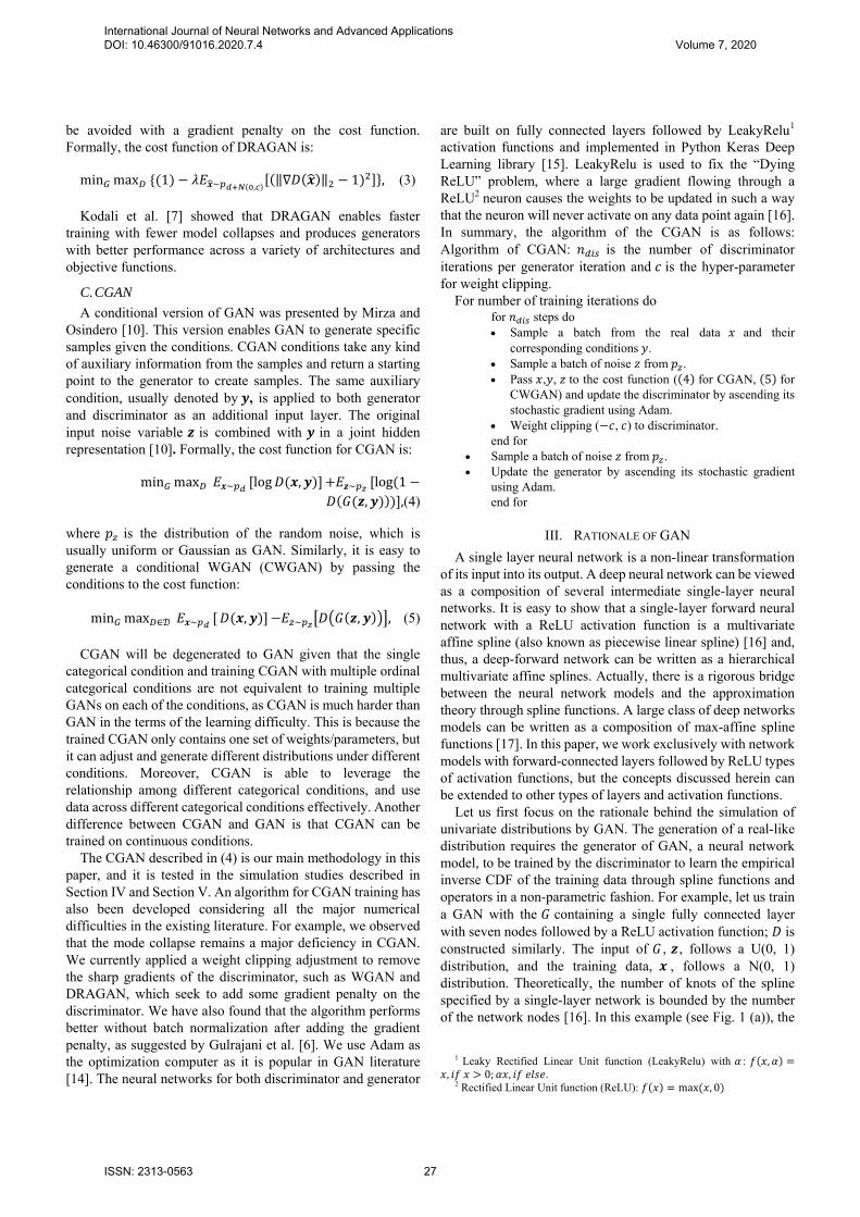
network, 𝐺, is trained to result in a piecewise linear spline function with two spline knots within [0, 1] (the meaningful domain of this mapping). The other five knots are either overlapped with the ones plotted in Fig. 1 (a) or located outside [0, 1]. It is worth pointing out that, here, the training data 𝒙 is independent from input 𝒛, and the network model cannot be trained by a simple loss function (such as the mean squared error or entropy) for a common supervised learning problem [15]. GAN, as an unsupervised learning method, provides a non-trivial alternative to learn the same mapping and match the inverse CDF of N(0, 1) from samples randomly extracted from U(0,1), which can be achieved as 𝐷 is trained simultaneously with 𝐺.

Next, in order to obtain a smoother spline approximation, we increase the node number of 𝐺 from seven to 100 for this example. Batch size and training iterations are increased as well. The results are provided in Fig. 1 (b), where the location and number of the spline knots are refined to obtain a smoother spline approximation and match the target function. Similarly, most of the spline knots are overlapped with the ones plotted in Fig. 1 (b) or located outside the support [0, 1]. As expected, this example does not evidence overfitting, as the CDF function of N(0,1) is a monotonic and smooth target function that can be fitted by a simple spline approximation.

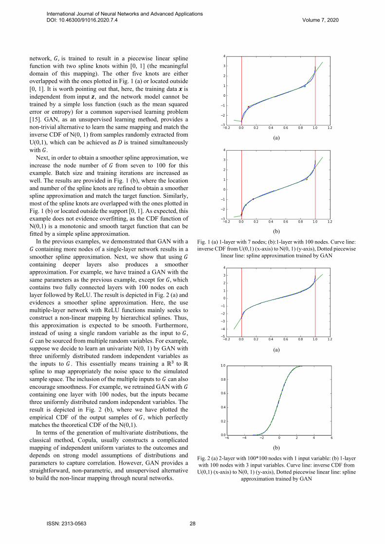
In the previous examples, we demonstrated that GAN with a 𝐺 containing more nodes of a single-layer network results in a smoother spline approximation. Next, we show that using 𝐺 containing deeper layers also produces a smoother approximation. For example, we have trained a GAN with the same parameters as the previous example, except for 𝐺, which contains two fully connected layers with 100 nodes on each layer followed by ReLU. The result is depicted in Fig. 2 (a) and evidences a smoother spline approximation. Here, the use multiple-layer network with ReLU functions mainly seeks to construct a non-linear mapping by hierarchical splines. Thus, this approximation is expected to be smooth. Furthermore, instead of using a single random variable as the input to 𝐺, 𝐺 can be sourced from multiple random variables. For example, suppose we decide to learn an univariate N(0, 1) by GAN with three uniformly distributed random independent variables as the inputs to 𝐺 . This essentially means training a ℝ to ℝ spline to map appropriately the noise space to the simulated sample space. The inclusion of the multiple inputs to 𝐺 can also encourage smoothness. For example, we retrained GAN with 𝐺 containing one layer with 100 nodes, but the inputs became three uniformly distributed random independent variables. The result is depicted in Fig. 2 (b), where we have plotted the empirical CDF of the output samples of 𝐺 , which perfectly matches the theoretical CDF of the N(0,1).

In terms of the generation of multivariate distributions, the classical method, Copula, usually constructs a complicated mapping of independent uniform variates to the outcomes and depends on strong model assumptions of distributions and parameters to capture correlation. However, GAN provides a straightforward, non-parametric, and unsupervised alternative to build the non-linear mapping through neural networks.

(a)

(b)

Fig. 1 (a) 1-layer with 7 nodes; (b):1-layer with 100 nodes. Curve line: inverse CDF from U(0,1) (x-axis) to N(0, 1) (y-axis), Dotted piecewise

linear line: spline approximation trained by GAN

(a)

(b)

Fig. 2 (a) 2-layer with 100*100 nodes with 1 input variable: (b) 1-layer with 100 nodes with 3 input variables. Curve line: inverse CDF from U(0,1) (x-axis) to N(0, 1) (y-axis), Dotted piecewise linear line: spline

approximation trained by GAN


Vol:14, No:6, 2020


Ope

n Sc

ienc

e In

dex,

Mec

hani

cal a

nd I

ndus

tria

l Eng

inee

ring

Vol

:14,

No:

6, 2

020

was

et.o

rg/P

ublic

atio

n/10

0112


ISSN: 2313-0563 28

In summary, both 𝐺 and 𝐷 of GAN, neural network models, can be written as a composition of spline operators. A smoother spline approximation can be obtained using deep layers, large number of nodes, and multiple random variables as inputs to 𝐺. CGAN builds non-linear mapping of the transformation of inputs into outputs on the same rationale as GAN. However, the key difference between CGAN and GAN is that CGAN uses additional variables, which are conditions inputted by the user. The condition variables are dependent on the training data. Thus, CGAN is a semi-supervised learning method.

IV. SIMULATION STUDY ON GAUSSIAN MIXTURE MODELS

In this section, we discuss the performance of the CGAN method on mixture of Gaussian distributions with various means and variances, including an example of extrapolation by CGAN. To assess the estimation of the heavy-tailed distributions by CGAN, we use Gaussian kernel density estimation [18], one of the most widespread non-parametric methods, as the benchmark model, where a cross-validation method is applied to find the best tuning parameters for the kernel estimation. The estimation is implemented in Python Scikit learning library [18].

In terms of the architectures of 𝐺 and 𝐷 in CGAN, we use a three-layer forward-connected network with 100+ nodes for each layer followed by LeakyRelu activation function for both 𝐺 and 𝐷. The inputs to 𝐺 are 30 random variables. Thus, we allow CGAN to be complex and capable enough to learn different kinds of multivariate distributions and time series. According to the Google Brain large-scale studies [14], most GAN models can exhibit a similar performance with enough hyper-parameter optimization and random restarts. Thus, we work with CGAN in the following subsections, where the hyper-parameters are set or trained in a setting similar to the one defined in the large-scale study from Google Brain [14].

A. Gaussian Mixture Model with Nominal Categorical Conditions

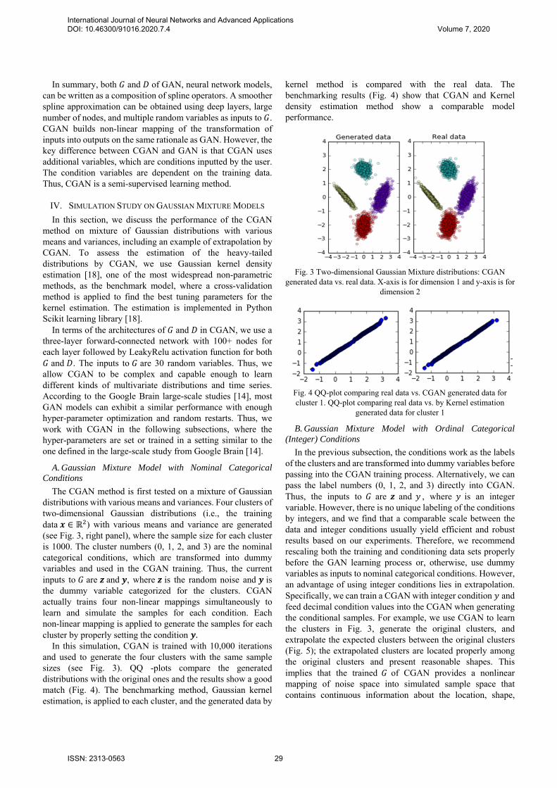
The CGAN method is first tested on a mixture of Gaussian distributions with various means and variances. Four clusters of two-dimensional Gaussian distributions (i.e., the training data 𝒙 ∈ ℝ ) with various means and variance are generated (see Fig. 3, right panel), where the sample size for each cluster is 1000. The cluster numbers (0, 1, 2, and 3) are the nominal categorical conditions, which are transformed into dummy variables and used in the CGAN training. Thus, the current inputs to 𝐺 are 𝒛 and 𝒚, where 𝒛 is the random noise and 𝒚 is the dummy variable categorized for the clusters. CGAN actually trains four non-linear mappings simultaneously to learn and simulate the samples for each condition. Each non-linear mapping is applied to generate the samples for each cluster by properly setting the condition 𝒚.

In this simulation, CGAN is trained with 10,000 iterations and used to generate the four clusters with the same sample sizes (see Fig. 3). QQ -plots compare the generated distributions with the original ones and the results show a good match (Fig. 4). The benchmarking method, Gaussian kernel estimation, is applied to each cluster, and the generated data by

kernel method is compared with the real data. The benchmarking results (Fig. 4) show that CGAN and Kernel density estimation method show a comparable model performance.

Fig. 3 Two-dimensional Gaussian Mixture distributions: CGAN generated data vs. real data. X-axis is for dimension 1 and y-axis is for

dimension 2

Fig. 4 QQ-plot comparing real data vs. CGAN generated data for cluster 1. QQ-plot comparing real data vs. by Kernel estimation

generated data for cluster 1

B. Gaussian Mixture Model with Ordinal Categorical (Integer) Conditions

In the previous subsection, the conditions work as the labels of the clusters and are transformed into dummy variables before passing into the CGAN training process. Alternatively, we can pass the label numbers (0, 1, 2, and 3) directly into CGAN. Thus, the inputs to 𝐺 are 𝒛 and 𝑦 , where 𝑦 is an integer variable. However, there is no unique labeling of the conditions by integers, and we find that a comparable scale between the data and integer conditions usually yield efficient and robust results based on our experiments. Therefore, we recommend rescaling both the training and conditioning data sets properly before the GAN learning process or, otherwise, use dummy variables as inputs to nominal categorical conditions. However, an advantage of using integer conditions lies in extrapolation. Specifically, we can train a CGAN with integer condition 𝑦 and feed decimal condition values into the CGAN when generating the conditional samples. For example, we use CGAN to learn the clusters in Fig. 3, generate the original clusters, and extrapolate the expected clusters between the original clusters (Fig. 5); the extrapolated clusters are located properly among the original clusters and present reasonable shapes. This implies that the trained 𝐺 of CGAN provides a nonlinear mapping of noise space into simulated sample space that contains continuous information about the location, shape,


Vol:14, No:6, 2020


Ope

n Sc

ienc

e In

dex,

Mec

hani

cal a

nd I

ndus

tria

l Eng

inee

ring

Vol

:14,

No:

6, 2

020

was

et.o

rg/P

ublic

atio

n/10

0112


ISSN: 2313-0563 29

mean, variance, and other statistics to generate and extrapolate conditional samples for different clusters.

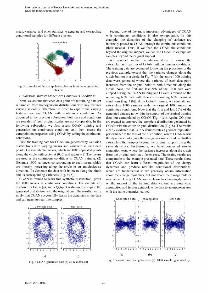
Fig. 5 Examples of the extrapolation clusters from the original four clusters

C. Gaussian Mixture Model with Continuous Conditions

Next, we assume that each data point of the training data set is sampled from homogeneous distributions with key features varying smoothly. Therefore, in order to capture the varying features, we use CGAN with continuous conditions. As discussed in the previous subsection, both data and conditions are rescaled if their original scales are not comparable. In the following subsection, we first assess CGAN training and generation on continuous conditions and then assess the extrapolation properties using CGAN by setting the continuous conditions.

First, the training data for CGAN are generated by Gaussian distributions with varying means and variances in each data point: (1) Generate the means, which are 1000 separated points along the circle with center at (0, 0) and radius = 2. The means are used as the continuous conditions in CGAN training. (2) Generate 1000 variances corresponding to each mean, which are linearly increasing along the circle in an anticlockwise direction. (3) Generate the data with its mean along the circle and its corresponding variances (Fig. 6 (b)).

CGAN is trained to learn this synthetic distribution, given the 1000 means as continuous conditions. The outputs are disclosed in Fig. 6 (a), and a QQ-plot is drawn to compare the generated distribution with the original one. The results clearly imply that CGAN successfully learns the dynamics in the data and can generate real-like samples.

(a) (b)

Fig. 6 CGAN generated data (a) vs. real data (b)

Second, one of the most important advantages of CGAN with continuous conditions is also extrapolation. In this example, the dynamics of the changing of variance are indirectly passed to CGAN through the continuous conditions (their means). Thus, if we feed the CGAN the conditions beyond the original support, we can use CGAN to extrapolate samples beyond the original support.

We conduct another simulation study to assess the extrapolation properties of CGAN with continuous conditions. The training data are generated following the procedure in the previous example, except that the variance changes along the x-axis but not in a circle. In Fig. 7 (a), the entire 1000 training data were generated where the variance of each data point increases from the original point to both directions along the x-axis. Next, the first and last 20% of the 1000 data were clipped during the CGAN training and CGAN is trained on the remaining 60% data with their corresponding 60% means as conditions (Fig. 7 (b)). After CGAN training, we simulate and extrapolate 1000 samples with the original 1000 means as continuous conditions. Note that the first and last 20% of the generated data are not within the support of the original training data, but extrapolated by CGAN (Fig. 7 (c)). Again, QQ-plots are created to compare the complete distribution generated by CGAN with the entire original distribution (Fig. 8). The results clearly evidence that CGAN demonstrates a good extrapolation performance at the tails of the distribution, where CGAN learns the dynamics underlying the change in variance and can further extrapolate the samples beyond the original support using the same dynamics. Furthermore, we have conducted similar simulation tests, where the variance increases along the x-axis from the original point at a faster pace. The testing results are comparable to the example presented here. These results show that CGAN can learn different magnitudes of the change dynamics and produce real-like conditional distributions, which are fundamental as we generally obtain information about the change dynamics, but not about their magnitude or mechanism. Using CGAN, we can learn the changing dynamics on the support of the training data without any parametric assumption and further extrapolate the data to an unknown area with the same dynamics learned.

(a) (b) (c)

Fig. 7 Variance increasing Scenario (a): 1000 samples generated by


Vol:14, No:6, 2020


Ope

n Sc

ienc

e In

dex,

Mec

hani

cal a

nd I

ndus

tria

l Eng

inee

ring

Vol

:14,

No:

6, 2

020

was

et.o

rg/P

ublic

atio

n/10

0112


ISSN: 2313-0563 30

CGAN with the original 1000 means as continuous conditions, (b): clipped data used in the CGAN training, (c) the original 1000 samples

Fig. 8 QQ-plot comparing the real data vs CGAN generated data.

V. SIMULATION STUDY ON TIME SERIES MODELS

In this section, we extend the use of CGAN to the learning and generation of time series data. Our focus is: (1) Vector autoregressive (VAR) time series with heavy-tailed underlying noise and region switching features. Heavy-tailed distributions simulate the behavior of real financial data. The region switching time series is a time series with different dependent structures from different time periods/regions used to simulate real market movements. They occasionally present dramatic breaks in their behavior, which are associated with events such as financial crises. (2) Multivariate GARCH time series with heavy-tailed underlying noise. Note that both VAR and GARCH models are usually used as parametric models to analyze financial time series, such as the modeling and prediction of stock rerun and GDP. We show that CGAN, as a nonparametric method, can learn dependence structures of these time series and simulate conditional predictive time series.

VAR model generalizes the univariate AR model and captures the linear dependent structures among multiple time series. The notation VAR (𝑝) indicates a vector AR of order 𝑝. Mathematically, the model can be defined as:

𝑿𝒕 𝒄 ∑ 𝒂 𝑿 𝜺 , (6)

where 𝒂 , 𝑖 1, … 𝑝 are the autocorrelation parameters, 𝒄 is a constant, and 𝜺𝒕 is the underlying noise. In Section V, we generate 𝑿𝒕 𝑥 , , 𝑥 , , 𝑡 1, … , 𝑇 , a 2-dimensional VAR time series with 𝑝 1 (or denoted as VAR(1)), as the training data for CGAN modeling. The underlying noises of 𝑿 are sampled from a T-distribution, which simulates the heavy- tailed distributions usually observed in the financial time series. Furthermore, we define the following terminologies as the main statistics to assess the first order correlations for the 𝑖th time series:1-lag autocorrelation

: 𝑐𝑜𝑟 , , ,

, ,,

Correlation with the 𝑗th time series

: 𝑐𝑜𝑟 , , ,

, ,,

Cross correlation between time series and time lags

: 𝑐𝑜𝑟 ,, , ,

, ,

.

Next, we define the second order 1-lag autocorrelation:

𝑣𝑜𝑙 , , ,

, ,

.

𝑣𝑜𝑙 , is used to assess the volatility dynamic of the GARCH time series, where the second order autocorrelation is usually larger than the first order. The second order correlation between time series (𝑣𝑜𝑙 ) and cross-correlation (𝑣𝑜𝑙 , ) can be defined similarly.

A. CGAN for VAR Time Series with Continuous Conditions

We assume that the training data follow a VAR (1) process with an underlying noise variable 𝜺𝒕. In order to test if CGAN can capture the underlying heavy-tailed noise distribution and its dynamic, we let 𝜺𝒕 follow a T-distribution with a degree of freedom (𝐷𝐹) of 20, and the variance of 𝜺𝒕 varies with the sum of the absolute value of 1-time-lag time series values. Formally, the training data is generated by (7):

𝑿𝒕 𝒂𝑿𝒕 𝟏 𝜺𝒕, (7)

𝒂 0.8, 0.6 , 𝜺𝒕 ~ 𝑇 𝑚𝑒𝑎𝑛 𝟎, 𝐶𝑜𝑣 𝑠𝑢𝑚 |𝑿𝒕 𝟏| ∙

1 00 1

, DF 20

Suppose we are at time t-1 and aiming to generate a 1-time-

horizon prediction of the time series at time t by CGAN. VAR model specifies the output variables linearly depending on the historical values and random noises; thus, we propose using the value of the previous time series, 𝑿𝒕 𝟏, as the conditions in the CGAN modeling of 𝑿𝒕. In this setting, the data format of both the training data and condition data is the following: Sample size x Number of Time Series = 20,000 x 2 (for this simulation example), where the condition data set is constructed by taking 1-time-lag sliding-window snapshot of the training data.

Here, CGAN was trained with 10,000 iterations. After the training, 500 conditional 1-time-horizon predictive distributions given 500 random selected conditions were generated and compared with the true ones. The distribution comparison is conducted in two manners: (a) For each condition, we draw a QQ-plot to compare the simulated conditional distribution and the true condition distribution. We fit a linear regression to assess the fit of the QQ-plot, where the R square and the slope of each comparison are saved and plotted in the histogram plot in Fig. 9. R squares and slopes cluster at 1 on x-axis, which indicates a good match. (b) We compare key statistics (mean, variance, skewness, and kurtosis) between the 500 generated conditional distributions by CGAN and the corresponding true conditional distributions. These statistics are depicted in Fig. 10. For example, the means and variances change in this simulation. The values from the true


Vol:14, No:6, 2020


Ope

n Sc

ienc

e In

dex,

Mec

hani

cal a

nd I

ndus

tria

l Eng

inee

ring

Vol

:14,

No:

6, 2

020

was

et.o

rg/P

ublic

atio

n/10

0112


ISSN: 2313-0563 31

conditional distributions (x-axis) are matched along a 45- degree line to the ones from CGAN’s generated conditional distributions (y-axis). This implies that CGAN is able to capture the autocorrelation parameters and the local changes in variance. Skewness and kurtosis are fixed in this simulation and, thus, located along a vertical line, and the intersection of this vertical line and the x-axis represents their true values. The skewness from CGAN is distributed around the true value 0 with a reasonable range of variation. The standardized kurtosis should be 0 in normal distribution. Nevertheless, the kurtosis value here should be larger than 0, as the underlying noise has a T-distribution with a degree freedom of 20. There are limited cases where the heavy-tail is underestimated, which is mainly due to the insufficient sample size of the training data. When we increase the sample size in our simulation, we found that the performance of CGAN is better in terms of capturing the key statistics of the training data, especially for the higher-order moments of the distribution. Similarly, we test VAR time series with other volatility changing dynamics. The results are comparable and indicate the CGAN is able to capture different types of dynamics of the underlying noise. In summary, we concluded that CGAN is able to learn the dependent structure of the VAR time series and the heavy tails of the underlying noise. CGAN can further generate the conditional 1-time horizon predictive distributions with the same key statistics as the training data given adequate sample sizes.

Fig. 9 Histogram of slope (1st column) and R square (2nd column) of the QQ plots comparing distributions generated by CGAN vs. VAR(1)

B. CGAN Modeling with Categorical Conditions for Region Switching Time Series

The region switching time series is a type of time series with dependent structures from different time periods. As we demonstrated in Section VI for real data analysis, both the autocorrelation parameters and the kurtosis of the time series data of equity returns exhibit large changes from the financial crisis to the normal period.

In order to capture the variant properties of distributions from different regions, we can apply CGAN with a categorical variable as the condition for each region, which essentially tells CGAN that samples of different categories have different distributions and dependent structures, and that the same category samples are homogeneous. However, when CGAN is assigned a categorical condition, it can only be trained to produce independent and identically distributed samples. In order to generate time series data with the original dependent structure, we need to reformat the training data by adding a

dimension for time. For example, we suppose that there are only two dimensions of the original training data (Sample size x Number of Time Series), then we add a time dimension by taking a T-time-lag sliding window snapshot. The updated training data format becomes Sample size x T x Number of Time Series. Thus, CGAN is able to learn all the dependent structure across time and different time series of the training data, and generate real-like time series.

Fig. 10 Mean (1st), variance (2nd), skewness (3rd) and kurtosis (4th) between the CGAN generated samples (y-axis) and real VAR

generated samples (x-axis) Specifically, in this simulation, there are two regions in the

time series, where the first 10,000 samples are from region 1, and the rest 10,000 samples are from region 2. Region 1 and region 2 have different VAR parameters for autocorrelation and underlying noises given below:

𝑿 𝒄 𝒂𝑿 𝜺 , (8)

Region 1: 𝒄 1, 0 , 𝒂 0.8, 0.8 , 𝜺𝒕 ~ 𝑇 𝑚𝑒𝑎𝑛

𝟎, 𝐶𝑜𝑣 1 0.50.5 1

, DF 6

Region 2: 𝒄 1, 0 , 𝒂 0.5, 0.5 , 𝜺𝒕 ~ 𝑇 𝑚𝑒𝑎𝑛

𝟎, 𝐶𝑜𝑣 1 0.30.3 1

, DF 12

As previously discussed, the training data are reformatted into Sample size x T x Number of Time Series = 20,000 x 2 x 2, where the time dimension is added by taking 1-time-lag sliding- window snapshot. Then, CGAN is trained on the reformatted data set with a categorical variable that serves as the condition for each region and10,000 iterations.

To assess the performance of CGAN learning, we begin by showing that CGAN can generate samples with the same dependence structure as the training data. During the CGAN training process, all the key statistics of the dependent structures are tracked. The tracking results are provided in Fig. 11, in which the first row shows the tracking results of the correlation statistics, the second row shows the volatility


Vol:14, No:6, 2020


Ope

n Sc

ienc

e In

dex,

Mec

hani

cal a

nd I

ndus

tria

l Eng

inee

ring

Vol

:14,

No:

6, 2

020

was

et.o

rg/P

ublic

atio

n/10

0112


ISSN: 2313-0563 32

statistics. The first column represents region 1, while the second column represents region 2. The horizontal straight lines are the corresponding true values of these statistics in the original training data. In Fig. 11, all of the first and second order autocorrelation, correlation and volatility statistics of the distributions generated by CGAN converge to their corresponding values specified by (8) for different regions, which implies that CGAN output data inherits all the input training data dependent features. Then, we show that CGAN is able to capture the underlying heavy-tailed distribution of the time series. We compare the CGAN generated data with the original data in Fig. 12 (a). The QQ-plots are generated to assess the goodness of fit between the generated and original distributions in both regions, and the results are reasonable (Fig. 12 (b)).

Fig. 11 VAR Tracking results of correlation and volatility over 10,000 CGAN learning iterations. X-axis is the iteration time. Y-axis is the

correlation/volatility statistics

(a) (b)

(c) (d)

Fig. 12 (a) CGAN generated data; (b) real data; QQ-plot Comparison for region 1 (c) and region 2 (d)

We have also conducted a similar test for VAR(1) with

Gaussian underlying noise and arrived at the same conclusion. In summary, we conclude that CGAN with categorical conditions is able to learn the correlation and volatility dynamics, and the underlying heavy-tailed distributions simultaneously.

C. CGAN for GARCH Time Series

In the previous subsections, we have demonstrated that CGAN is able to learn the dependent features and the heavy- tailed distribution of the underlying noise of VAR-type time series. In this subsection, we extend our discussion to the GARCH time series, which usually have a dependent structure in the variance. Formally, a multivariate GARCH (p, q) time series 𝑿 , 𝑡 1, … 𝑇 is:

𝝈 𝒄 ∑ 𝒂 𝑿𝟐 ∑ 𝒃 𝝈𝟐 , 𝑿 ~ 𝑁 𝟎, 𝝈 ), (9)

where 𝒂 , 𝒃 , 𝑖 1, … 𝑝 are the parameters, 𝒄 is the constant and 𝜺𝒕 is usually a white noise. As in the VAR model, we use GARCH (1, 1) as an example in the following simulation studies.

We begin with a quick review of the conditions used in the previous sections. For mixture Gaussian distributions, we pass a variable containing information of their mean and the changing trend of variance into CGAN. For VAR models, we used the historical 1-time-lag time series values as the conditions, which essentially pass the sample means of the conditional distribution to the CGAN training. However, GARCH time series usually has a small magnitude of the dependent structure of the means, but a strong correlation in the variance. Thus, the best condition to generate the GARCH time series values at time t is the variance at time t, 𝝈 . However, the variance information at t is usually unknown at time t-1. In order to make a 1-time-horizon prediction, we leverage the GARCH volatilities at time t, 𝝈 𝒄 ∑ 𝒂𝒊𝑿∑ 𝒃𝒊𝝈 as our “prior” information, and treat them as the conditions for CGAN. However, unlike parametric GARCH model, CGAN does not require an assumption of distribution, and can automatically capture the cross-correlations across multiple time series. In the future research, we will consider applying the long short-term memory (LSTM) layers [2] into 𝐺 to extract the historical volatility information automatically. Please note that GARCH volatility 𝝈 only depends on the information up to t-1, so it is known at t-1.

In the following CGAN simulations, besides conditioning on


Vol:14, No:6, 2020


Ope

n Sc

ienc

e In

dex,

Mec

hani

cal a

nd I

ndus

tria

l Eng

inee

ring

Vol

:14,

No:

6, 2

020

was

et.o

rg/P

ublic

atio

n/10

0112


ISSN: 2313-0563 33

𝝈 , we also show the simulation results conditioning on 𝝈 for comparison purposes. Specifically, the training data structure is Sample size x Number of TS = 10,000 x 2, and the GARCH parameters are:

𝝈𝒕

𝟐 𝒄 𝒂𝑿𝒕 𝟏𝟐 𝒃𝝈𝒕 𝟏

𝟐 , (10)

𝑿𝒕 ~ 𝑻 𝟎, 𝝈𝒕𝟐 ∙ 1 0

0 1, 𝐷𝐹 20 , 𝒄 0.3, 0.3 , 𝒂

0.3, 0.3 , 𝒃 0.6, 0.6

CGAN is trained with 10,000 iterations, and there are two CGAN models: CGAN trained conditional on 𝝈 (denoted as CGAN𝝈𝒕

), and on 𝝈 (denoted as CGAN𝝈𝒕 𝟏). To assess model

performance, we randomly sample 500 conditions of𝝈 , and use CGAN𝝈𝒕 𝟏 to generate 500 conditional distributions given these conditions. In addition, we calculate 500 𝝈 from the 𝝈 , leveraging the GARCH volatilities, and use these 𝝈 as conditions to generate 500 conditional distributions by CGAN𝝈𝒕

. Finally, all these conditional distributions either from CGAN𝝈𝒕 𝟏

or CGAN𝝈𝒕 are compared with the conditional

distributions specified by (10). The results are provided in Fig. 13, which implies that both CGAN𝝈𝒕 𝟏

and CGAN𝝈𝒕 are able to

learn the changing dynamics of the variance, but CGAN𝝈𝒕

outperforms the CGAN𝝈𝒕 𝟏 as there is a more clear matching trend at 45 degree line, demonstrating the importance of using an appropriate condition in CGAN. Moreover, both can capture the heavy tails of the underlying noise, as the kurtosis is concentrated at around a positive value indicating a heavier tail than N(0, 1).

We conduct similar tests on GARCH time series with different parameters and the results are comparable. In summary, we conclude that CGAN is able to learn the dynamics of GARCH time series, the heavy tail of the underlying noise, and it is also able to generate reasonable 1- time horizon prediction.

(a)

(b)

Fig. 13 Mean (1st), variance (2nd), skewness (3rd) and kurtosis (4th) between the generated conditional distributions (y-axis) and the true

ones (x-axis); (a) for CGAN𝛔𝐭 and (b) for CGAN𝛔𝐭 𝟏

VI. REAL DATA ANALYSIS

In this section, we apply the proposed CGAN method on two real data sets 1-day stock returns and macroeconomic index data; the former is closer to the GARCH time series and the latter is similar to a VAR time series. CGAN is trained on the same algorithm and neural network architectures of the simulation study. In addition, a backtesting [11] is conducted show that CGAN is able to outperform HS and ES in the calculation of VaR.

A. Equity 1-Day Return

We download equity spot prices for WFC and JPM from November 1, 2007 to November 1, 2011 from Yahoo Finance [19]. Then, 1-day absolute returns are calculated and used as training data. As an example, the time series of the 1-day return of JPM is presented in Fig. 14, in which the time series experienced many sharp changes during the financial crisis of 2008.

If we separate the data by crisis period (the so-called stressed period around November 2007–2009) and post-crisis period (the normal period November 2009–2011) we can observe that the joint distribution of WFC and JPM 1-day absolute return has longer tails and larger variances than the ones in the normal period. Moreover, the correlation structure is also different (Fig. 15 (a)). This pattern is similar to the region switch time series discussed in section V, where the key data features are changed from time to time.

In market risk analysis, financial institutions usually separate the analysis of the post-crisis period from the crisis period, which leads to the calculation of a general VaR for normal periods and stressed VaR for stressed periods. With CGAN, we can easily separate the data learning and generation of the stressed and the normal periods using an indicator of periods as a categorical condition. In order to generate time series data, we add a dimension to the original data structure, as we did in


Vol:14, No:6, 2020


Ope

n Sc

ienc

e In

dex,

Mec

hani

cal a

nd I

ndus

tria

l Eng

inee

ring

Vol

:14,

No:

6, 2

020

was

et.o

rg/P

ublic

atio

n/10

0112


ISSN: 2313-0563 34

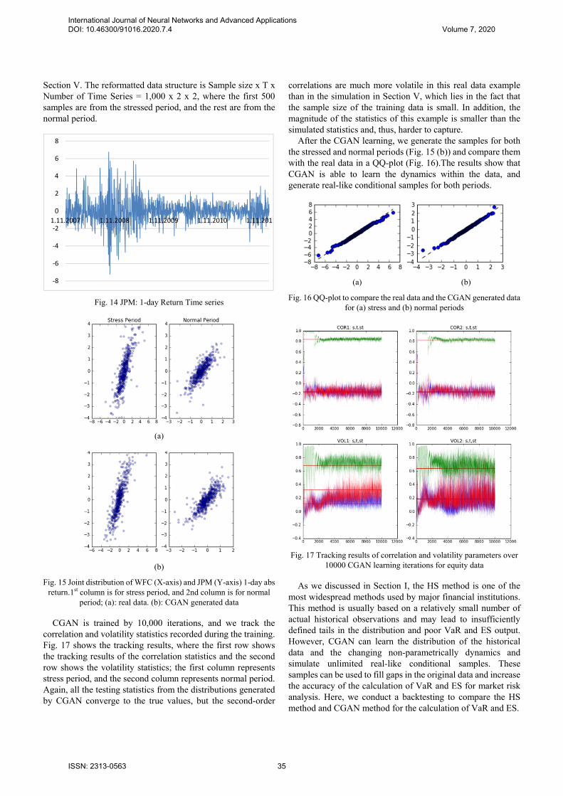
Section V. The reformatted data structure is Sample size x T x Number of Time Series = 1,000 x 2 x 2, where the first 500 samples are from the stressed period, and the rest are from the normal period.

Fig. 14 JPM: 1-day Return Time series

(a)

(b)

Fig. 15 Joint distribution of WFC (X-axis) and JPM (Y-axis) 1-day abs return.1st column is for stress period, and 2nd column is for normal

period; (a): real data. (b): CGAN generated data

CGAN is trained by 10,000 iterations, and we track the correlation and volatility statistics recorded during the training. Fig. 17 shows the tracking results, where the first row shows the tracking results of the correlation statistics and the second row shows the volatility statistics; the first column represents stress period, and the second column represents normal period. Again, all the testing statistics from the distributions generated by CGAN converge to the true values, but the second-order

correlations are much more volatile in this real data example than in the simulation in Section V, which lies in the fact that the sample size of the training data is small. In addition, the magnitude of the statistics of this example is smaller than the simulated statistics and, thus, harder to capture.

After the CGAN learning, we generate the samples for both the stressed and normal periods (Fig. 15 (b)) and compare them with the real data in a QQ-plot (Fig. 16).The results show that CGAN is able to learn the dynamics within the data, and generate real-like conditional samples for both periods.

(a) (b)

Fig. 16 QQ-plot to compare the real data and the CGAN generated data for (a) stress and (b) normal periods

Fig. 17 Tracking results of correlation and volatility parameters over 10000 CGAN learning iterations for equity data

As we discussed in Section I, the HS method is one of the

most widespread methods used by major financial institutions. This method is usually based on a relatively small number of actual historical observations and may lead to insufficiently defined tails in the distribution and poor VaR and ES output. However, CGAN can learn the distribution of the historical data and the changing non-parametrically dynamics and simulate unlimited real-like conditional samples. These samples can be used to fill gaps in the original data and increase the accuracy of the calculation of VaR and ES for market risk analysis. Here, we conduct a backtesting to compare the HS method and CGAN method for the calculation of VaR and ES.

‐8

‐6

‐4

‐2

0

2

4

6

8

1.11.2007 1.11.2008 1.11.2009 1.11.2010 1.11.2011


Vol:14, No:6, 2020


Ope

n Sc

ienc

e In

dex,

Mec

hani

cal a

nd I

ndus

tria

l Eng

inee

ring

Vol

:14,

No:

6, 2

020

was

et.o

rg/P

ublic

atio

n/10

0112


ISSN: 2313-0563 35

Suppose we have 1 unit of WFC and JPM stock in our testing portfolio. First, the 1-day 99% VaR and ES of this portfolio is calculated by HS for the stressed period (November 2007- 2009), and the normal period (Nove4mber 2009-2011), which are provided in Table I. We assume that the data are iid, and the ES is calculated as the average of the tail data values instead of using a weighted average. Next, we plot the left 5% tail of the PnL distributions of this portfolio in both the stressed and normal periods, where the tails have not been sufficiently described by the relatively small number of actual historical data (see Fig. 18).

Second, we use CGAN to learn the historical data for both the stressed and normal periods, and generate a real-like conditional sample set with a sample 50 times larger than the original. Then, we calculate VaR and ES on these larger generated data (Table I). Fig. 19 shows that the large dataset generated by CGAN results in a clear tail of the distribution.

Next, additional historical data for WFC and JPM stock prices from November 1, 2011-November 1, 2015 (around 1000 business days) are downloaded from Yahoo Finance to implement the backtesting. Since no financial crises were recorded in this period, we use VaR and ES from the normal period (in Table I) as our measurement in the backtesting. The expected breaches over 1000 days for 1-day 99% VaR is 10 days, given the iid assumption. There are 22 breaches using the 99% VaR from HS, whereas CGAN results in only eight breaches. In addition, the actual 1-day 99% ES over these 1000 days is -4.04, but ES from HS is only -3.06, whereas ES from CGAN is -4.20. Table II shows that the HS method may lead to an underestimated measurement of the portfolio loss, and CGAN outperformed the HS method in the calculation of VaR and ES in this example.

A. Economic Feorecasting Model

CGAN can be an appealing alternative in the forecasting and modeling of macroeconomic time series. Large-scale econometric models like MAUS represent the conventional approach and resort to thousands of equations to model correlation structures. Each equation is individually estimated or calibrated, and forecasts are produced quarterly and used as inputs of the subsequent quarterly forecasts. CCAR requires multiple economic forecasts during different hypothetical economic scenarios. CGAN-based economic model provides an alternative approach by which multiquarter forecasts can be produced simultaneously, and the randomness of the output allows the modelers to assess the distributions of the forecasted paths. For example, we have downloaded five popular macroeconomic index data from Q1 1956 to Q3 2016 from the U.S. Census Bureau [23], namely real Gross Domestic Product (GDP), unemployment rate (unemp), Federal fund rate, Consumer Price Index (CPI), and 10-year treasury rate [23]. All these five raw time series are transformed into standardized stationary time series with a sample mean of 0 and a standard deviation of 1. After the transformation, the whole dataset contains five variables over 242 quarters. In order to simulate time series, the initial training dataset (5 variable x 242 quarter) is transformed into the training data for CGAN (230 sample x 5

variable x 13 quarter) by taking a sliding-window snapshot of 13 quarters, as in the simulation study in Section V. It is worth noting that the training dataset is relatively smaller in size compared with the dimensions of the variables and quarter. Therefore, the training is more challenging and requires a greater number of iterations for each convergence.

TABLE I

99% 1-DAY VAR AND ES OF THE TESTING PORTFOLIO CALCULATED BY HS

AND CGAN

HS method CGAN

Stress Period

Normal Period

Stress Period

Normal Period

VaR (USD) -4.98 -2.53 -7.11 -3.40

ES (USD) -6.28 -3.06 -9.04 -4.20

Fig. 18 Left 5% tail of the PnL distribution of the testing portfolio for stress and normal periods

Fig. 19 Left 5% tail of the PnL distribution generated by CGAN (with a simple size 50 times larger) for stress and normal periods

TABLE II

BACKTESTING RESULTS AND COMPARISON OF 99% ES VALUES

HS CGAN

99% VaR -2.53 -3.40

Breaches over 99% VaR 22 8

Expected breaches at 99% level 10 10

99% ES -3.06 -4.20

Actual 99% ES -4.04 -4.04

In this section, we use the first four quarters of data as the conditions in CGAN modeling to predict the last nine-quarter time series outputs. Thus, the inputs for generator consist of white noises and continuous conditions and it is a dataset containing 230 sample x 5 variable x 4 quarters. The output is the predictive time series dataset containing 230 sample x 5


Vol:14, No:6, 2020


Ope

n Sc

ienc

e In

dex,

Mec

hani

cal a

nd I

ndus

tria

l Eng

inee

ring

Vol

:14,

No:

6, 2

020

was

et.o

rg/P

ublic

atio

n/10

0112


ISSN: 2313-0563 36

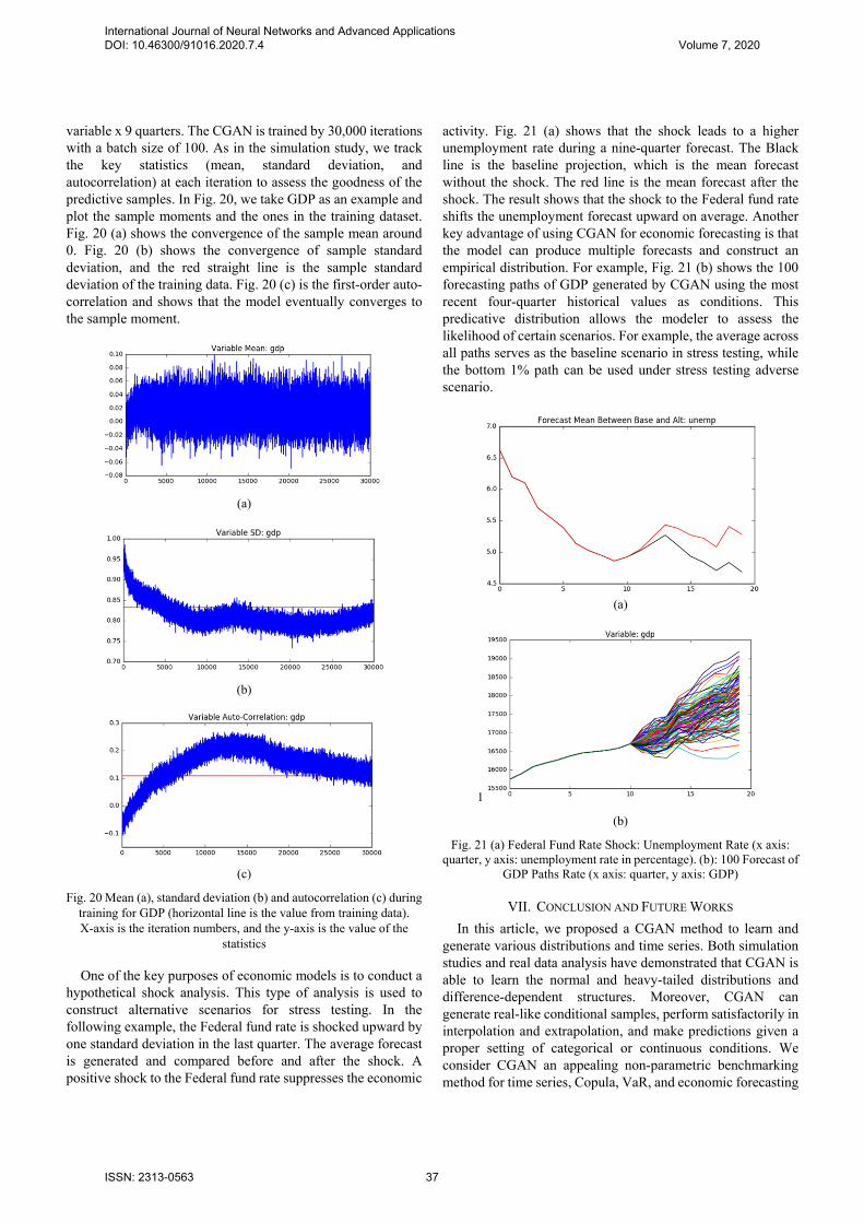
variable x 9 quarters. The CGAN is trained by 30,000 iterations with a batch size of 100. As in the simulation study, we track the key statistics (mean, standard deviation, and autocorrelation) at each iteration to assess the goodness of the predictive samples. In Fig. 20, we take GDP as an example and plot the sample moments and the ones in the training dataset. Fig. 20 (a) shows the convergence of the sample mean around 0. Fig. 20 (b) shows the convergence of sample standard deviation, and the red straight line is the sample standard deviation of the training data. Fig. 20 (c) is the first-order autocorrelation and shows that the model eventually converges to the sample moment.

(a)

(b)

(c)

Fig. 20 Mean (a), standard deviation (b) and autocorrelation (c) during training for GDP (horizontal line is the value from training data). X-axis is the iteration numbers, and the y-axis is the value of the

statistics

One of the key purposes of economic models is to conduct a hypothetical shock analysis. This type of analysis is used to construct alternative scenarios for stress testing. In the following example, the Federal fund rate is shocked upward by one standard deviation in the last quarter. The average forecast is generated and compared before and after the shock. A positive shock to the Federal fund rate suppresses the economic

activity. Fig. 21 (a) shows that the shock leads to a higher unemployment rate during a nine-quarter forecast. The Black line is the baseline projection, which is the mean forecast without the shock. The red line is the mean forecast after the shock. The result shows that the shock to the Federal fund rate shifts the unemployment forecast upward on average. Another key advantage of using CGAN for economic forecasting is that the model can produce multiple forecasts and construct an empirical distribution. For example, Fig. 21 (b) shows the 100 forecasting paths of GDP generated by CGAN using the most recent four-quarter historical values as conditions. This predicative distribution allows the modeler to assess the likelihood of certain scenarios. For example, the average across all paths serves as the baseline scenario in stress testing, while the bottom 1% path can be used under stress testing adverse scenario.

(a)

1

(b)

Fig. 21 (a) Federal Fund Rate Shock: Unemployment Rate (x axis: quarter, y axis: unemployment rate in percentage). (b): 100 Forecast of

GDP Paths Rate (x axis: quarter, y axis: GDP)

VII. CONCLUSION AND FUTURE WORKS

In this article, we proposed a CGAN method to learn and generate various distributions and time series. Both simulation studies and real data analysis have demonstrated that CGAN is able to learn the normal and heavy-tailed distributions and difference-dependent structures. Moreover, CGAN can generate real-like conditional samples, perform satisfactorily in interpolation and extrapolation, and make predictions given a proper setting of categorical or continuous conditions. We consider CGAN an appealing non-parametric benchmarking method for time series, Copula, VaR, and economic forecasting


Vol:14, No:6, 2020


Ope

n Sc

ienc

e In

dex,

Mec

hani

cal a

nd I

ndus

tria

l Eng

inee

ring

Vol

:14,

No:

6, 2

020

was

et.o

rg/P

ublic

atio

n/10

0112


ISSN: 2313-0563 37

models. First, we consider that future works can provide for more

complicated neural network layers for the discriminator and generator. For example, deep convolutional layers have been embraced in in the field of computer vision. GAN with convolutional networks has already been developed and proved an appealing alternative to improve GAN learning processes and perform dimension deductions [20]. In addition, recurrent neural networks and LSTM layers have been recently introduced to formulate volatility and model stochastic processes [2]. Similarly, LSTM layers have been successfully applied to GAN for stock market prediction on high frequency data [22].

Second, instead of using the weight clipping adjustment to the discriminator, we can adopt the gradient penalty method as in the WGAN-GP [6] and DRAGAN [7]. Different cost functions of GAN can be applied as well, such as LSGAN [9], Non-saturating GAN [14], and Boundary equilibrium GAN [21].

Third, future works should discuss the choices of the conditions for CGAN. For example, we can train the CGAN conditional on a joint distribution of continuous and categorical variables and enable CGAN to capture both the global and local changing dynamics of the data. However, this approach may render the learning process more difficult and, thus, require more advanced neural network structures to build the model.

Finally, more simulation studies can be performed to investigate the ability of CGAN to capture the second-order correlation of the time series. For instance, we could add the second-order terms in the training data and compel CGAN to learn the first-order and second-order terms simultaneously, which implies adding more weight of the second-term in the cost function of CGAN. Furthermore, we can use CGAN to learn and generate more stochastic processes, such as QG- models and volatility surface models. Some works have successfully discussed neural network models, but not the GAN method specifically [2], [22].

REFERENCES [1] R.S. Tsay. Analysis of Financial Time Series. John Wiley & Sons, Inc,

2002. [2] R. Luo, W. Zhang, X. Xu, and J. Wang. “A Neural Stochastic Volatility

Model”. arxiv preprint arXiv:1712.00504v1, 2017. [3] I. Goodfellow, J. Pouget-Abadie, M. Mirza, B. Xu, D. Warde-Farley, S.

Ozair, A. Courville, and Y. Bengio. “Generative Adversarial Nets.” Advances in Neural Information Processing Systems 27, Curran Associates, Inc., 2014, pp 2672-2680.

[4] W. Fedus, M. Rosca, B. Lakshminarayanan, A.M. Dai, S. Mohamed, and I. Goodfellow. “Many Paths To Equilibrium: GANs Do Not Need To Decrease a Divergence at Every Step” arXiv preprint arXiv: 1710.08446v3, 2018.

[5] M. Arjovsky, S. Chintala, and L. Bottou. “Wasserstein GAN.” arXiv preprint arXiv:1701.07875v3, 2017.

[6] I. Gulrajani, F. Ahmed, M. Arjovsky, V. Dumoulin, and A. Courville. “Improved Training of Wasserstein GANs.” arXiv preprint arXiv: 1704.00028, 2017.

[7] N. Kodali, J. Abernethy, J. Hays, Z. Kira. “On Convergence and Stability of GANs.” arXiv preprint arXiv:1705.07215, 2017.

[8] T. Salimans, I. Goodfellow, W. Zaremba, V. Cheung, A. Radford and X. Chen. “Improve Techniques for Training GANs.” arXiv preprint arXiv 1606.03498v1, 2016.

[9] X. Mao, Q. Li, H. Xie, R.YK Lau, Z. Wang, and S. Paul Smolley. “Least

squares generative adversarial networks.” arXiv preprint ArXiv: 1611.04076, 2016.

[10] Mehdi Mirza and Simon Osindero. “Conditional Generative Adversarial Nets.” arXiv preprint ArXiv:1411.1784v1, 2014.

[11] Global Association of Risk Professionals (GARP). 2016 Financial Risk Manager (FRM) Part II: Market Risk Measurement and Management, Fifth Edition. Pearson Education, Inc., 2016.

[12] Ernst & Young. “Fundamental review of the trading book (FRTB): the revised market risk capital framework and its implementations”. www.ey.com/Publication/vwLUAssets/ey-fundamental-review-of-the-trading-book/$FILE/ey-fundamental-review-of-the-trading-book.pdf. 2016

[13] Board of Governors of the Federal Reserve System. “Comprehensive Capital Analysis and Review 2012: Methodology and Results for Stress Scenario Projections”, www.federalreserve.gov. 2012.

[14] M. Lucic, K. Kurach, M. Michalski, S. Gelly, and O. Bousquet. “Are GANs Created Equal? A Large-Scale Study” arXiv preprint ArXiv: 1711.10337v3, 2018.

[15] Keras: The Python Deep Learning library, keras.io. Date of access: 20 Sep 2018

[16] H. Magus and O. Christoffer. “Feedforward neural networks with ReLU activation functions are linear splines” PhD diss., Lund University, 2017.

[17] R. Balestiero and R. Baraniuk. “Mad Max: Affine Spline Insights into Deep Learning” arXiv preprint ArXiv:1805.06576v5, 2018.

[18] Kernel Approximation. Scikit-learn v0.20.2. scikit-learn.org/stable/modules/kernel_approximation.html,2019

[19] Yahoo Finance. finance.yahoo.com. Date of access: 20 Aug 2018. [20] A. Radford, L. Metz and Soumith Chintala. “Unsupervised

Representation Learning with Deep Convolutional Generative Adversarial Networks” arXiv preprint ArXiv:1511.0643, 2015.

[21] D. Berthlot, T. Schumm, and L.Metz. “BEGAN: Boundary equilibrium GAN” arXiv preprint ArXiv: 1703.10717, 2017.

[22] X. Zhou, Z. Pan, G. Hu, S. Tang and C. Zhao. “Stock Market Prediction on High Frequency Data Using Generative Adversarial Nets”. Mathematical Problems in Engineering, Volume 2018, Article ID 4907423, 11 pages, 2018.

[23] U.S. Census Bureau. www.census.gov. Date of access: 10 Aug 2018.


Vol:14, No:6, 2020


Ope

n Sc

ienc

e In

dex,

Mec

hani

cal a

nd I

ndus

tria

l Eng

inee

ring

Vol

:14,

No:

6, 2

020

was

et.o

rg/P

ublic

atio

n/10

0112

73

Creative Commons Attribution License 4.0 (Attribution 4.0 International, CC BY 4.0)

This article is published under the terms of the Creative Commons Attribution License 4.0 https://creativecommons.org/licenses/by/4.0/deed.en_US

International Journal of Neural Networks and Advanced Applications DOI: 10.46300/91016.2020.7.4 Volume 7, 2020

ISSN: 2313-0563 38

time series simulation by conditional generative

Documents