The submitted manurcript has been authored by a contractor of the U. S. Government under contract No. W-31-104ENG-38. Accordingly, the U. S. Government retains a nonexclusive. royalty-free license to publish or reproduce the published form of this contribution. or allow others to do SO, for U. S. Government purposes.

APPLICATION OF NEURAL NETWORKS TO SEISMIC ACTIVE CONTROL

Yu Tang Reactor Engineering Division Argonne National Laboratory

Argonne, Illinois

+ -

ABSTRACT An exploratory study on seismic active control using an

artificial neural network (ANN) is presented in which a single- degree-of-freedom (SDF) structural system is controlled by a trained neural network. A feed-forward neural network and the backpropagation training method are used in the study. In backpropagation training, the learning rate is determined by ensuring the decrease of the error function at each training cycle. The training patterns for the Bura l net are generated randomly. Then, the trained ANN is used to compute the control force according to the control algorithm. The control strategy proposed herein is to apply the control force at every time step to destroy the build-up of the system response. The ground motions considered in the simulations are the N21E and N69W components of the Lake Hughes No. 12 record that occurred in the San Fernando Valley in California on February 9, 1971. Significant reduction of the structural response by one order of magnitude is observed. Also, it is shown that the proposed control strategy has the ability to reduce the peak that occurs during the first few cycles of the time history. These promising results assert the potential of applying ANNs to active structural control under seismic loads.

INTRODUCTION "Active Structural Control" is to equip the structure with an

active control device to counteract or minimize the motion experienced by the structke so that the dynamic response of the structure is reduced. This idea was first proposed by Yao in 1972 (Yao, 1972). Since then, this area of research has received considerable attention. Recently, considering the importance of this area, the U.S. Panel on Structural Control Research was

formed in 1991 (Soong, Masri, and Housner, 1991) and the International Association for Structural Control was formed in 1994 (Housner, Soong, and Masri, 1994). So, the active structural control is right now a booming research area. Many control laws, linear and nonlinear, have been proposed and studied, and two types of mechanical control systems, the active bracing (ABS) and variable stiffness method (VSM), have been laboratory tested. Despite all these developments, there are still problems that must be addressed before it is implemented to real structures. For example, the structural modelingmors and time delay. The majority of the control algorithms proposed are based on the optimal control theory which usually assumes that the system under control can be precisely mathematically modeled. This is almost an unattainable condition for civil structures. Also, it is assumed that all operations in the control can be performed instantaneously. In reality,- time needs to be consumed in the data process, in the computation, and in the activation of the control device.

Because an ANN is not sensitive to the noise present in the input data, it can handle the modeling error more gracefully, and also because an ANN involves only the matrix multiplications and additions, it can cut down the process time. Or, if the software simulation is not fast enough, an ANN may be fabricated in a very large-scale integration (VLSI) for real time response. Once the network has been trained, a chip can be constructed. The chip is then placed into electronics by which a real-time operation can be achieved. Therefore, an ANN is a good candidate for the implementation of the active control. The potential of applying ANNs with the backpropagation (BP) training algorithm to active control has been explored by Wen, et al. (1992), and the result is promising. However, in their paper, the time delay problem was not addressed. In this study,

DISCLAIMER

Portions of this document may be illegible in electronic image products. lmages are produced from the best available original document.

the simple control strategy proposed in Tang (1995) is employed herein. This strategy is heuristic in nature and is a non-optimal type of control rule. In other words, there is no objective function to be optimized. The basic idea behind this control strategy is the same as that of the pulse control proposed by Udwadia and Tabaie (1981), i.e., to destroy the gradual rhythmic build-up of the structural response; however, details of the algorithm and implementation are quite different from those of Udwadia and Tabaie (1981). It can be implemented for a closed-loop control or an open-closed loop control. In this paper, it is assumed that a closed-loop control is implemented.

The effectiveness of the control strategy used herein is demonstrated by numerical examples in which a SDF system under seismic excitations is studied. The dynamic responses of the SDF system with and without control are compared, and also the controlled system responses obtained by the control strategy used herein are compared with those obtained by control strategy proposed in Wen, et al. (1992). The results show that the control strategy used herein is superior to that of Wen, et al., and it is able to produce a significant peak reduction for the peak occurring during the first few cycles of the time history, an ability the linear control laws lack (Gattlli, Lin, and Soong, 1994). The ground motions considered in the examples are the N21E and N69W components of the Lake Hughes No. 12 record that occurred in the San Fernando Valley in California on February 9, 1971. The duration of the record is 36.76 seconds, and the magnitudes for the two components considered are 0.902 g for N21E and 0.711 g for N69W. However, the magnitudes of the accelerations are scaled down to 0.0775 g in the numerical examples.

ARTIFICIAL NEURAL NETWORKS An artificial neural network is an information-processing

system based on observed behavior of biological nervous systems. A neural net consists of a large number of simple process elements (PES). Each PE is connected to another PE by means of direct communication links, each with an associated weight. It is these weights that represent the information stored in the system and hold the key to the functioning of an ANN. Among many different types of A N N s , the feedforward multilayer perceptron with the backpropagation algorithm, the so-called backpropagation (BP) net, is the most widely used supervised learning algorithm in neural network applications.

The structure of a typical PE in a BP net is shown in Fig. 1 in which (xl, x2 ,..., xd, is the input vector, b is the bias, (wl, wu...,wn) is the associated weight vector, I is the intermediate scalar, f o is the so-called activation function, and y is the output from the PE. Specifically, I is computed by the equation

Y = f o (2)

In this study, the activation function used is given by

2 1 + e - '

f(x) = - - 1 (3)

The architecture of an example of a BP net consisting of an input layer, a hidden layer and an output layer, is shown in Fig. 2.

In the training process, an error function is used to assess the performance of the net. This error function is defined by

(4)

in which P is the number of patterns in the training set, and tpj and opj(w) are the target and actual output of the jth output neuron for the pth pattern, respectively. o . is denoted as a function of w to indicate the dependency of tfe network outputs on the weight vector w. The weight vector is updated by

where a = the learning rate which is a constant in the range of (0 1) in a standard BP algorithm, and Vqw) is the gradient vector. Note that in Eq. (2) the weights are updated after all of the patterns in the training set have been passed through the net. A common variation is to update the weights after each training pattern is presented. In this study an adaptive BP algorithm is used, Le., the learning rate is changing during training. The algorithm is based on the gradient phase of the SGRA algorithm proposed by Miele, et al. (1970). The advantage of this algorithm is that the decrease of error function at each epoch is guaranteed; otherwise, the program stops. The capability of BP nets for approximating a continuous mapping is proved by the "Kolmogorov mapping neural network existence theorem" (Funahashi, 1989, and Hecht-Nielsen, 1987). Also, Cybenko (1989) has proved that a continuous function may be arbitrarily well approximated by feedforward neural networks with a nonlinear continuous activation function. For more details about the BP net the reader is referred to Freeman and Skapura (1991) and Hecht-Nielsen (1990).

The BP net used in this study has five PES for the input layer, eight PES each for the two hidden layers, and one PE for the output layer, This BP net needs to be trained before it can be used in the application. The preparation details for the training patterns can be found in Tang (unpublished report 1995).

n

i = l I = wixi + b

and y is obtained from the equation

SYSTEM CONSIDERED x j = x(t) ' .

Description of System Considered A linear single-degree-of-freedom (SDF) system is used herein

to demonstrate the application of an ANN to seismic active control. The system is shown in Fig. 1. It is the same one demonstrated experimentally for the active structural control in the paper by Chung. et al. (1988). The structural properties of the SDF system are listed below:

Mass, m: 16.69 lb-se&in. Structure Stiffness, k 7934 lb/in. Natural Frequency, &: 3.47 Hz Damping Factor, 5: 5%

For more details on the experimental setup, the reader is referred to the paper by Chung, et al. (1988). Note that the linear control theory was used in that study.

CONTROL STRATEGY

equation of motion is given by For a linear SDF system subjected to base excitation, the

X(t) + 4Zf&X(t) + 4Z*f;x(t) = -%,(t) (6)

in which a dot indicates the derivative with respect to time, & and t; are the natural frequency and damping ratio of the system, respectively, and x,(t) is the effective base excitation consisting of two parts. One part is the control force, denoted by Fc(t), and the other is the ground accekation, denoted by x,(t), i.e.,

F,(t) %,(t) = %,(t) + - m

where m = the mass of the SDF system. If the Duhamel integral is used to solve Eq. (3) and the

piecewise-linear interpolation for the loading is assumed, it can be shown, e.g., Craig, Jr. (1981), that the system response at t=ti, x(tJ and x(ti), may be determined from the information of x(ti- At), x(t-Ar), %,(ti-At), and %,(ti> where At is the data sampling rate. In this study it is assumed that the sensors provide the information about x(t) and x(t) at a rate of 0.01 second (assume a closed-loop control). These measured data are fed into a trained ANN to estimate the control force needed. The input vector for the ANN includes five elements: the displacement, velocity and load at the preceding time step, and the displacement, velocity and load at the current time step. They are denoted by xl, x2, x3, x4 and x5, respectively, i.e.,

XI = x(t-At)

XZ = d( td t )

xq = X(t)

The output from an ANN is a single PE that contains the information of the load, %,(t).

For each time interval, say from t=$ to t=ti+At, an ANN is used twice sequentially to perform the following computations:

First:

Input to ANN

~2 = *($-At)

x3 = x(ti>

x4 = X(tJ

XS = %,(ti-At)

output of ANN

Y = %,(ti)

Second:

Input to A N N

x1 = x(t9

x2 = X(t9

x3 = 0

(9)

x4 = 0

x5 = "(ti>

output of ANN

y = Fc(ti+At)hn

to compute the control force, Fc(ti+At), needed for t=ti+At. Conceptually, the first computation, Eq. (9), is to ask the ANN what the load is that produces the system response, x(tJ and x(tJ, and the second computation, Eq. (lo), is to ask the ANN what the necessary force is that can produce the zero displacement and velocity at t=g+At. Note that at t=O, ~ ( 0 ) = x(0) = f,(O) = Fc(0) = 0 and at t = 0 + At, Fc(O+At) = 0 are assumed, and the control algorithm is stopped when

x1=x2=x3=x4=xs=0 are detected. If the strategy is implemented for an open-closed loop control, the first computation is not

needed because x,(ti) is provided by the sensor, and x,(ti) can be constructed by making use of Eq. (7).

control strategy. The effectiveness of the control law is demonstrated by numerical examples. The results show that the system response is reduced by one order of magnitude, and the control strategy used has the ability to produce a significant peak reduction for the peak occurring during the first few cycles of the time history.

NUMERICAL EXAMPLES In this section the dynamic responses of the SDF system

described above subjected to base excitations are studied. The trained ANN is used to compute the control force. Two earthquake motions are used herein for the input base excitations. They are the N21E and N69W components of the Lake Hughes No. 12 record that occurred in the San Fernando Valley in California on February 9, 1971. The duration of the earthquake is 36.76 seconds. The magnitudes of the two records were scaled down to 0.0775 g. The plots of these two time histories are shown in Figs. 3 and 4, respectively. For discussion purposes, the first time history is referred to as Base Motion 1, and the second time history is referred to as Base Motion 2.

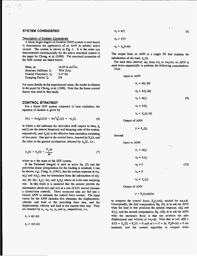
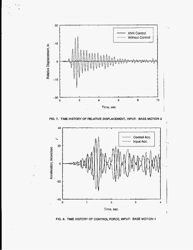
The flow chart for the control scheme using an ANN is depicted in Fig. 5. For Base Motion 1, the time histories of the relative displacement, x(t), with and without control are compared in Fig. 6. The corresponding information for using Base Motion 2 is presented in Fig. 7. For clarity, only the first 10 seconds of the responses are plotted. Examining Figs. 6 and 7, one can see clearly the effectiveness of the ANN control; the structural response is drastically reduced by one order of magnitude. Also, one may notice the significant reduction for the first peak of the response, which, as mentioned above, cannot be produced by the linear control laws. The control force in terms of the acceleration, F,(t)/m, for Base Motion 1 is shown in Fig. 8; also plotted in the same figure by the dotted line is the input base motion for comparison. One can see that the control acceleration is about 180 degrees out of phase with the input base motion.

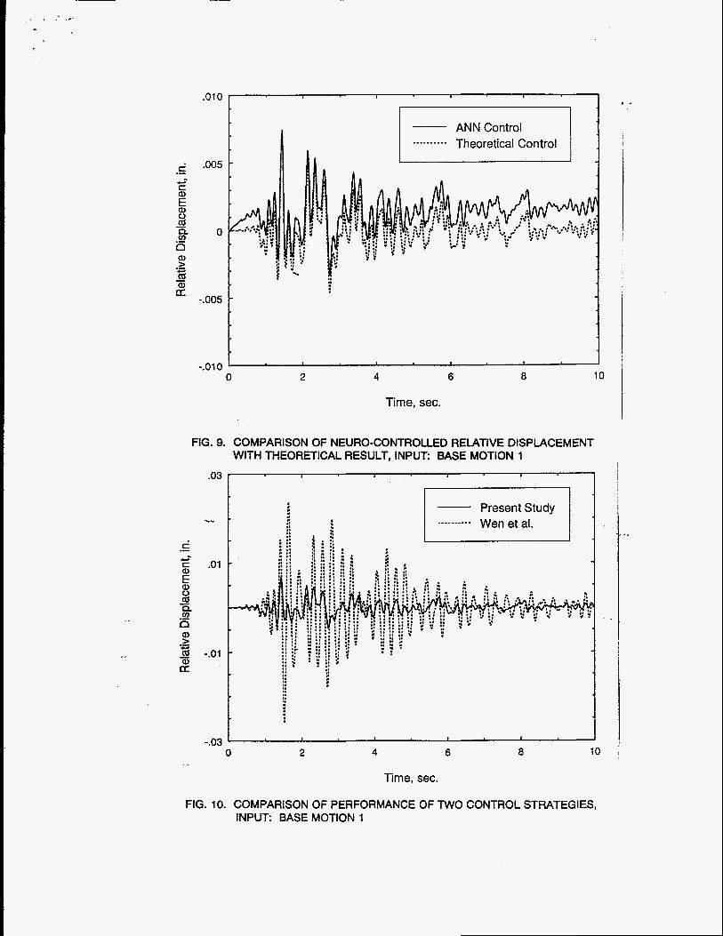
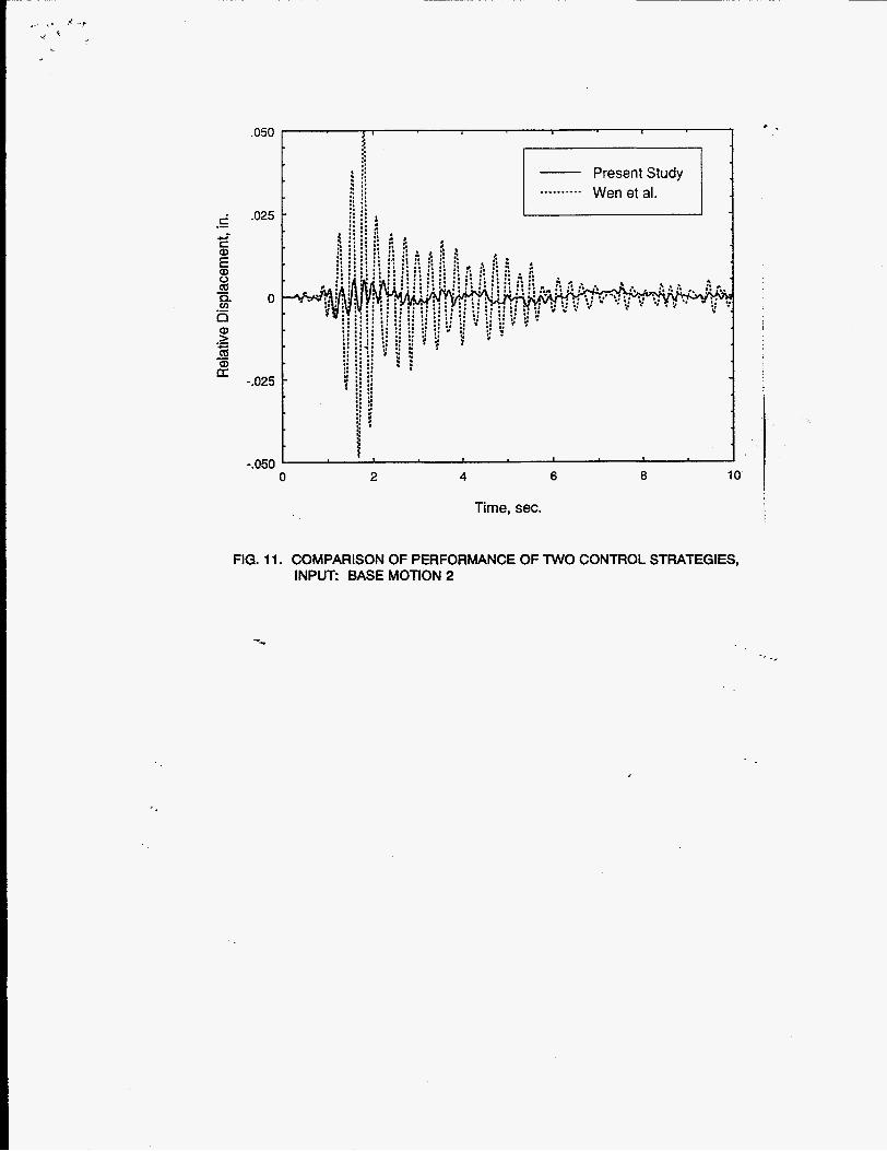
It should be mentioned that the control force for the proposed control strategy may be computed by a closed form solution (Tang, unpublished report 1995). One should therefore be interested in the comparisons of the structural response controlled by the ANN with that controlled by a theoretical controller in which the control force is computed by the closed form solution. Such a comparison is presented in Fig. 9 for Base Motion 1. One can see that, except for the constant drift between the two curves, these two curves are almost identical. Also, the theoretical results are compared with those obtained by the control strategy proposed in Wen, et. al. (1992) in which the control force is set equal in magnitude but in the opposite direction of the product of the mass and ground acceleration. These comparisons are presented in Figs. 10 and 11 for Base Motions 1 and 2, respectively. One can see. that the control strategy used herein is superior to that of Wen, et al.

ACKNOWLEDGEMENT This paper was supported by the U.S. Department of Energy,

Technology Support Programs under Contract W-31-109-Eng-38.

REFERENCES

Chung, L. L., Reinhorn, A. M., and Soong, T. T., 1988, "Experiments on Active Control of Seismic Structures," Journal of Engineering Mechanics, ASCE, Vol. 114, No. 2, pp. 241-256.

Craig, Jr., R. R., 1981, "Structural Dynamics: An Introduction to Computer Method," John Wiley & Sons, Inc. New York, NY.

Cybenko, G., 1989, "Approximation by Superpositions of a Sigmoidal Function," Math. Control Signal Systems, Vol. 2, pp.

Freeman, J. A, and Skapura, D. M., 1991, "Neural Networks: 303-314.

Algorithm, Applications and Programming Techniques, Addison-Wesley Publishing Co., Reading, MA.

Funahashi, K., 1989, "On the Approximate Realization of Continuous Mapping by Neural Networks," Neural Networks,

Gafflli, V., Lin, R. C., and Soong, T. T., 1994, "Nonlinear Control Laws for Enhancement of Structural Control Effectiveness," Proceedings, 5th U.S. National Conference on Earthquake Engineering, Chicago, IL, pp. 971-975.

Hecht-Nielsen, R., 1987, "Kolmogorov's Mapping Neural Network Existence Theorem," Proceedings, 1st International Conference on Networks, Vol. 111, pp. 11-14, IEEE Press, New York.

Hecht-Nielsen, R., 1990, "Neurocomputing," Addison-Wesley Publishing Co., Reading, MA.

Housner, G. W., Soong, T. T., and Masri, S. F., 1994, "Second Generation of Active Structural Control in Civil Engineering," Final Program and Abstracts, First World Conference on Structural Control, LQS Angeles, CA.

Miele, A., Pritchard, R. E., and Damoulakis, J. N., 1970, "Sequential Gradient-Restoration Algorithm for Optimal Control Problems," Journal of Optimization Theory and Application, Vol.

Soong, T. T., Masri, S. F., and Housner, G. W., 1991, "An Overview of Active Structural Control Under Seismic Loads", Earthquake Spectrum, Vol. 7, No. 3, pp. 483-505.

Udwadia, F. E., and Tabaie, S., 1981, "Pulse Control of Single Degree-of-Freedom System," Journal of Engineering Mechanics,

Vol. 2, NO. 3, pp. 183-192.

5, NO. 4, pp. 235-282.

ASCE, Vol. 107, NO. 6, pp. 997-1009. CONCLUDING REMARKS

A study of seismic active control is presented. The control algorithm implemented is based on a heuristic, non-optimal

Wen, Y. IC, Ghaboussi, J., Venini. P., and Nikzad, K., 1992, "Control of Structures Using Neural Networks," Proceedings, U.S.lItalylJapan Workshop on Structural Control and Intelligent Systems, Sonento, Italy, pp. 232-251.

Yao, J. T. P., 1972, "Concept of Structural Control," Journal of the Structural Divbwn, ASCE, Vol. 98, No. 7, pp. 1567-1574.

A -

b (bias)

A

- - y = f ( I ) .....

Xn

(Activation Function) (Output) (Inputs) (Weights)

FIG. 1. A TYPICAL PE IN BACKPROPAGATION NETS

-- n I !

Hidden Layer

FIG. 2. ARCHITECTURE OF A BACKPROPAGATION NET

!

30 -

15 -

0

I

-15 -

Time, sec.

FIG. 3. N21 E COMPONENT OF LAKE HUGHES NO. 12 RECORD

301 . ' 4 8 ' . I * . 1 * - . . I

-- 15

0

-1 5

-30 A 0 10 20 30

Time, sec.

i

40 '

FIG. 4. N69W COMPONENT OF LAKE HUGHES NO. 12 RECORD

P

External

0

- r Structure Structural

-. 1

Excitation

0

Response

Control Force I

Artificial Neural t Network (ANN)

FIG. 5. FLOW CHART OF ANN CONTROL FOR THE EXAMPLE PROBLEM

: :

ANN Control Without Control

I I I I

2 4 6 a 10

Time, sec

FIG. 6. TIME HISTORY OF RELATIVE DISPLACEMENT, INPUT: BASE MOTION 1

.30

ANN Control -

.15 I I . . * .. .. .. .e .. .. :: :: ::

Without Control __.__..___

0

-.15

I I I I -.30 ’ !

I 0 2 4 6 a 10

Time, sec

FIG. 7. TIME HISTORY OF RELATIVE DISPLACEMENT, INPUT: BASE MOTION 2

FIG. 8. TIME HISTORY OF CONTROL FORCE, INPUT BASE MOTION 1

-L

20

0

-20

-40 0 1 2 3 4

Time, sec. I

.010 1 t I

t f

-.010 ' I

0 2 4 6 8 10

Time, sec.

FIG. 9. COMPARISON OF NEURO-CONTROLLED RELATIVE DISPLACEMENT WITH THEORETICAL RESULT, INPUT: BASE MOTION 1

.03 - I i

- ti

c .01 .- - - 2 8

n

a Q v)

- _- .- .b-

,, 9 -.01 ;

-.03 I I I I t I 0 2 4 6 8 10

Time, sec.

FIG. 10. COMPARISON OF PERFORMANCE OF TWO CONTROL STRATEGIES, INPUT BASE MOTION 1

,.. < * ? - r 4 s

0 2 4 6 8 10 1 i Time, sec. I

i

FIG. 11. COMPARISON OF PERFORMANCE OF TWO CONTROL STRATEGIES, INPUT BASE MOTION 2