APPLICATION OF PROBABILISTIC FRACTUREMECHANICS TO ALLOCATION OF NDT

FOR NUCLEAR PRESSURE VESSELS

M. Bergman*, B. Brickstad*, P. Dillström*, F. Nilsson**

SKI 13.2-1203/90-90152

SA/FoU-Rapport 91/09

AB SVENSK ANLÄGGNINGSPROVNING

The Swedish Plant InspectorateBox 49306 • S-100 28 Stockholm • Sweden

Telefon 08-617 40 (X)Telefax 08-51 70 43

APPLICATION OF PROBABILISTIC FRACTUREMECHANICS TO ALLOCATION OF NDT

FOR NUCLEAR PRESSURE VESSELS

M. Bergman*, B. Brickstad*. P. Dillström*, F. Nilsson

SKI 13.2-1203/90-90152

SA/FoU-Rapport 91/09

**

* The Swedish Plant Inspectorate ** Department of Solid MechanicsBox 49 306 Royal Institute of TechnologyS-100 28 Stockholm, Sweden S-100 44 Stockholm, Sweden

Aug 1991

AB SVENSK ANLÄGGNINGSPROVNINGThe Swedish Plant Inspectorate

Box 49306,100 28 Stockholm • SwedenTfn Int.+46 8-617 40 00

Telex 12124 anprovsTelefax +46 8-65170 43

1

APPLICATION OF PROBABILISTIC FRACTURE MECHANICS TO

ALLOCATION OF NDT FOR NUCLEAR PRESSURE VESSELS

M. Bergman*, B. Brickstad*, P. Dillström*, F. Nilsson**

•The Swedish Plant Inspectorate **Department of Solid Mechanics

Box 49306 Royal Institute of Technology

S-100 28 Stockholm, Sweden S-100 44 Stockholm, Sweden

AbstractIn order to study whether there are considerable differences in fracture probability between dif-

ferent regions in a reactor pressure vessel a limited probabilistic fracture mechanics (PFM)

study is carried out. Two different regions (crack geometries) are considered and the fracture

and leakage probabilities are calculated for a number of load cases. The loading is assumed to

be deterministic while most of the other quantities are assumed to be of random character. The

fracture probabilities are very dependent of assumption made for the fracture toughness distri-

bution , but the mutual order of the fracture probabilities of the two regions seemed to be rela-

tively unaffected by this. Of the transients considered, the cold overpressurization event is by

far the most dangerous event. A sensitivity analysis shows however that this result is heavily

dependent ofihe transition temperature of the material. The leakage probabilities are in most ca-

ses much lower than the fracture probabilities indicating that consequence considerations are not

very important for NDT allocation purposes.

2

Table of contentsAbstract 1

Table of contents 2

Nomenclature 3

1. Introduction 5

2. Scope of the study 6

2.1. General outline 6

2.2. Regions chosen for study 7

2.3. Transients 8

3. Modelling 9

3.1./-calculations 9

3.2. Material assumptions and deterministic fracture analysis 10

3.3. Probabilistic assumptions and relations 13

3.4. Simplification 15

3.5. Kf - and limit load solutions 15

3.6. Calculation of leakage rates 16

3.7. Numerical realization 18

4. Input data 19

4.1. Stress distributions 19

4.2. Fracture toughness properties 20

4.3. Size distribution of initial defects 21

4.4. Crack growth calculations 22

4.5. Crack incidence rates 23

5. Results 24

5.1. Basic set of indata 24

5.2. Some sensitivity studies 26

6. Discussion 28

7. Conclusions 29

References 30

Appendix, basic fracture and leakage probabilities 32

3

Nomenclature

a exponent in crack growth resistance curve

a crack depth

a* crack growth constant

OQ crack depth before stable crack growth

OQO crack depth before subcritical crack growth (fatigue or SCC)

Aw leakage area on inner surface

A^ leakage area on outer surface

Cmm ,C^, £bm £bb coefficients for leakage area calculations

d wall thickness

Aa crack growth increment

\c(°oo) subcritical crack growth (fatigue or SCC)

E Young's modulus

fa probability density function for crack depth

fito R6 function

/ , 0 probability density function for70

h temperature dependence of Jo

h a temperature dependence of/,

H Heaviside step function

J J- integral

/„ characteristic toughness value of the material

/ Q ^ highest Jo value for instability of through the thickness crack

/ t a highest Jo value for instability of surface crack

•Aton- lowest Jo value for crack arrest to occur

Ja arrest toughness

JR crack growth resistance

Ko reference stress intensity factor for fatigue crack growth

K, stress intensity factor

Kla crack arrest toughness value according to ASME Sect XI

Kle fracture toughness according to ASME Sect. XI

Klcta upper shelf level of fracture toughness according to ASME Sect. XI

K crack aspect ratio

/ crack length

Lr limit load parameter

n exponent in fatigue crack propagation law

v Poisson's ratio

p pressure

Pfe probability of catastrophic failure due to one crack

Plt probability of leakage due to one crack

P, (OQ ) probability of crack growth initiation

PJ^OQ ) probability of unstable crack growth without any arrest

PU{QQ ) probability of stable crack growth through the thickness

P/ep failure probability for preservice defects for the itth loading case

Pfk

ti failure probability for inservice defects.for the itth loading case

Ptk probability for the itth loading case to occur

Q primary load

QL plastic limit load

R stress ratio of fatigue loading

Rt internal radius of pressure vessel

am membrane stress

ab bending stress

RTNaT nil-ductility transition temperature

p interaction factor

T temperature

To reference temperature

5

1. Introduction

The inservice inspection of Swedish reactor pressure vessels have up to date followed the gene-

ral programs given in ASME Sect. XI [1]. From time to time it has been argued that these are

not the optimal programs in that the regions chosen for inspection are not necessarily the most

critical ones for the total safety of the vessel. Quantitative arguments in this debate have, how-

ever, so far been scarce. An obvious candidate for methodology is probabilistic fracture

mechanics (PFM). PFM has mostly been used to aid licensing decisions either for new nuclear

reactors (the Marshall report [2]) or for specific problems like the pressurized thermal shock

(PTS). For the latter problems a specific method and computer code was developed, the VISA-

code [3].

The work described here is part of a larger project initiated and sponsored by the

Swedish Nuclear Power Inspectorate. This project has the object to investigate whether there

are grounds to change the current choice of regions for inspection. The task is a difficult one

since many different factors affect the risk of rupture or leakage of the reactor vessel and the

probabilistic distributions of these are poorly known. It was from the outset clear that PFM

could not provide the final answers to the questions asked but rather be a helpful tool in sorting

out the influence of different variables.

A novelty of the entire project in comparison with earlier considerations of the subject

was the intention to consider that failure or leakage in different regions may lead to different

consequences. Thus it was from the outset clear that consequence analyses were to be conside-

red. These are not dealt with in the present report but one requirement on the final results of the

PFM-analyses was that their format should be compatible with the probabilistic safety analyses.

It should be stressed that for the current purpose the absolute values of the failure pro-

babilities are not important but it is rather the relative ones that are of interest. This relaxes some

of the difficulties normally associated with PFM analysis. The main object is to establish the or-

der of priority between the different regions. If it can be shown that this order is relatively in-

sensitive to uncertainties of the input data, then the order may be considered as reliable even if

the absolute probability may be poorly known.

With regard to the specific objects as outlined here we have chosen to keep the probabi-

listic calculations as simple as possible and not to rely on sophisticated PFM computer codes.

Instead the analysis is based on fairly simple expressions and on one-dimensional numerical

integrations. The aim of the study presented here was to establish a methodology and apply to a

few regions in a specific BWR reactor (the Oskarshamn unit 2, 02) vessel in order to judge

whether a discrimination of the importance of the different regions is at all possible.

6

2. Scope of the study

2.1. General outline

The possible consequences of a failure or a leakage of a BWR reactor vessel may roughly be

categorized into the following types:

i) Loss of coolant.

ii) Secondary effects on the primary piping.

iii) Missile effects on the primary piping and the containment

From consultations with system analysts it was decided to primarily direct the present work to

the determination of leakage probabilities of the following categories:

a) Catastrophic: Leakage rate > 16 000 kg/s.

b) Large: 2 000 kg/s < leakage rate < 16 000 kg/s.

c) Moderate: 30 kg/s < leakage rate < 2 000 kg/s.

d) Insignificant: leakage rate £ 30 kg/s.

Simple estimates showed that leakage of categories a) and b) can only occur if rapid crack

growth and total failure of the vessel happens. Thus there is no reason from a fracture mecha-

nics view-point to distinguish between these two categories. Leakages of third category c) can

occur if an initially long crack grows stably through the thickness. Calculations discussed later

will show that leakages even for very long cracks fall at the low end of this category.

The situation to analyse is the following. A certain inspection region, say the core re-

gion, is considered. With some probability one crack or more may be present in the region.

These cracks can be either preservice or inservice defects. Such a crack may grow further due

fatigue or stress corrosion cracking. When it reaches a certain critical size depending on the

fracture toughness and the loading conditions it may start to grow stably. This growth may

eventually lead to unstable growth and catastrophic failure or to stable growth through the wall

and leakage of some size. Since Swedish nuclear reactor vessels are inspected on a ten year ba-

sis this period will be chosen for the crack growth calculations.

Let Pp be the mean incidence rate of the preservice defects. P^ can be larger than unity

and in such a case denotes the expected number of preservice defects in the region. Likewise let

Pä be the mean rate of incidence of inservice defects. We here define occurrence as to have

happened if a crack penetrates the cladding for the latter case. Further let Pjkip be the failure

probability because of a preservice defect for the kwh loading case and P(ktl the corresponding

probability for an inservice defect P,k is the probability that the particular loading case occurs.

Then to first order the total probability of catastrophic failure for the considered region is

Pf= (2.1)

With a corresponding notation we obtain the total probability of leakage as

Pt = (2.2)

Here P£p denotes the leakage probability due to a preservice defect for the k\h loading case and

/}*, the leakage probability due to an inservice defect. In these equations the failure probabili-

ties P/tp etc. and the leakage probabilities ?uP etc. were determined by analytical means as

described in section 3 below. The other quantities in (2.1) and (2.2) were instead estimated by

qualitative methods. Again, in view of the goal of the projects if there was no particular reason

to assign different values to specific variable in different regions this was not done. Thus, the

contribution of this variable to the discrimination is small.

Comer crack in steam line nozzle Surface crack in core region

cladding / I

Fig. 1. Crack geometries chosen for consideration

22. Regions chosen for study

In this first study a few regions were chosen mainly in order to judge whether a differentiation

is possible. The first region under consideration (I) is the part of the cylindrical wall away from

geometrical disturbances but possibly subjected to the neutron irradiation. We call this the core

g

region and axial surface cracks on the inside of the wall are considered. The depth of the crack

is denoted a and the length /. Circumferential cracks are subjected to much lower stresses and

the fracture probability in this region will be wholly dominated by the axial cracks.

The second geometry (II) chosen for study is that of a comer crack in a steam line

nozzle. The crack is here taken as semi-circular with radius a. The two geometries are sketched

in Fig. 1.

23. Transients

The transients for which the different regions were evaluated were chosen according to the

following considerations. For each region a few transients belonging to the categories normal

and upset were chosen which were expected to give the most severe loading of the transients

that almost certainly occur.

T[°C]

- -300

1—I—I 1—I—\500 ' 1 8 0 0 time [s]

Fig. 2. Pressure and temperature time history in core region during steam line break.

One load case, the steam line break (SLB), belonging to the category faulted was chosen

to judge the effects of a severe but unlikely transient. In addition a very severe transient, cold

over pressurization during outage (COP), which is extremely unlikely was chosen for study.

Each transient was specified in manner shown in Fig. 2. for the SLB. The main characteristics

of the remaining transients are summarized in Table 1. In this table the assumed probabilities

P,k that these transients occur during an inspection interval are given.

Region

Core region

Comer crack in

steam line

nozzle

Transient

Turbine trip (TT)

Reactor isolation

(RI)

Steam line break

(SLB)

Cold over pressuri-

zation during outage

(COP)

Reactor isolation

(RI)Level increase

during shut-down

(LI)

Steam line break

(SLB)

Cold over pressuri-

zation during outage

(COP)

Pressure

[MPa]

7.0 (const.)

7.7 (const)

7.0-0.0

8.0 (const)

7.7 (const)

7.0-1.0

7.0-0.0

8.0 (const)

Temperat.

[°C]

272 - 237

286

286-50

50

286

286-180

286 - 50

50

Heat transfer

coefficient

104

-

IOMO 4

-

KP-IO4

1.5-104

Probability

P,k

1.

1.

103

105

1.

1.

io-3

105

Table 1. Characteristics of transients considered.

3. Modelling

3.1. J-calculations

Fully elasto-plastic finite element calculations are in general necessary in order to obtain accu-

rate values of the /-integral. Within this project it was, however, not realistic to perform such

detailed calculations for the many cases that had to be considered. Instead, an approximate met-

hod based on option 1 of the R6-method [4] was used. According to this the /-value is given by

Kf (1 - v2)EfadL)- P)2 (3.1)

where K, is the stress intensity factor, £ the Young's modulus, v Poisson's ratio and

(3.2)

(3.3)

10

with Q being the primary load and QL the plastic limit load, p is a factor that accounts for the

interaction between primary and secondary loads and is calculated according to the method des-

cribed in [5]. For the different loading cases and regions J was calculated as function of the

crack depth a with the aspect ratio K = loll held constant.

32. Material assumptions and deterministic fracture analysis

We consider a specific region and crack orientation and shape. The first step in the analysis is to

calculate J(a) according to the procedure described above for the loading given by the actual

transient. It is now assumed that initiation and stable propagation of the crack growth can be

described by a JR -curve according to

J(a) <Joh(T-To), no growth. ( 3 4 )

J(a) =JK = 7 0 [ l + S(Aa) H(T-T0)] h(T-T0 ) , during growth. ( 3 5 )

It is for simplicity assumed that the information about the random nature of the material fracture

properties is contained in the single scalar parameter 7 0 . 7 is the temperature and 70 a reference

temperature describing the transition between brittle and ductile failure as defined below. H is

the Heaviside step function and it is thus assumed that no stable crack growth occurs for tempe-

ratures below 70. This was motivated by the observation made by Nilsson et al [6] that in the

transition region cleavage fracture tends to occur for surface cracks even if laboratory speci-

mens do exhibit a ductile growth behaviour. g(Aa) describes the increase of crack growth

resistance due to crack growth in the upper shelf region and was determined from experimental

data as discussed below.

Below 7*0 the temperature dependence h is assumed the same as in the curve for Kk in

ASME Sect. XI [1]. 70 in tum is the temperature when the Klc - curve of ASME reaches the

upper shelf level (Ktcus = 220 MPam"2). Thus

To =RTNm +56°C, (3.6)

h= (Klc(T)/Klcu,)2 =

(3.7)= [0.273 + 4.77- 10-3Ar+1.002- 10'4A72 + 8.29- 10"7A73]2, f o r 7 < 7 0 .

Here A7= T-RTNDT , where is RTNDT the nil-ductility transition temperature. For temperatures

larger than 70 the results by Östensson [7] were used. In his investigation the temperature de-

pendence of Jc as well as JR was studied in a large interval. At 70 the Jc values coincided quite

well with the upper shelf value of ASME while at larger temperatures a decrease was found. A

linear fit to the results of [7] was made here so that

11

h = 1 - (T-To)/T\ for T >T0, T*= 6 4 0 ° C . (3.8)

The crack growth resistance was also estimated from [7] with the result

S(Aa) = (1 + Ao la*)*-1, with a = 0.0002 m and a = 0.533. (3.9)

If the crack starts to grow unstably this is assumed to lead to catastrophic failure unless arrestoccurs. This event is assumed to happen if J(a) falls below a value Ja, the crack arrest tough-ness. Possible dynamic effects are neglected. In the lower shelf and transition region a tempera-ture dependence corresponding to the Kla curve of ASME Sect XI is assumed. Thus

(3.10)

with

(3.11)

, 2 -

(3.12)ha = (Kia(T)/Klcia)

2 =

= {01321 + 6.08- lCT3exp[0.026(7"-rfl+190)]}2, for T < Ta

Very little data are available for the crack arrest toughness in the upper shelf region. We makethe simple assumption that the temperature dependence of the crack arrest value is the same asfor the crack growth initiation value i. e.

Ja=Joh(J-Ta)=Joha{T-Ta) forT>Tfl. (3.13)

It is firstly of interest to calculate possible crack growth initiation. From the assumptionswe obtain that for a given crack depth OQ initiation happens

J(ao)ZJoh(T-T0),

or equivalently expressed

I

J0 ' h(T-T0)' (3.15)

Next we consider when unstable crack growth can occur. For a crack to become un-stable at the crack depth a eq. (3.5) has to be satisfied together with the condition

12

TJ Q h ( T T 0 ) ^ . (3.16)

Eqs. (3.5) and (3.16) form an equation system from which the solution J a - and Aa can be ob-

tained. With the assumed form (3.9) forJR this system can be solved explicitly to give

(3.17)

da J ' (3.18)

If Jo falls below J0^(a0) a crack of initial depth a0 = a-Aa can become unstable. This requiresthat (3.15) is satisfied for the crack depth a0. If (3.15) is not satisfied unstable crack growth cannot happen from a crack with depth %

Let us now consider under which circumstances a crack may grow stably through thewall thickness d. Obviously Jo must be larger than the value corresponding to instability butlower than the initiation value. Furthermore for continued growth eq. (3.5) must be satisfied atevery crack depth between OQ and d. This leads to the condition

fa) < /o < Min J(ä)(3.19)

Should JQ,, (a0) be less than JOin(ao)no stable growth through the thickness is possible.When an elliptical crack emanating from the inner surface grows so that its deepest point

reaches the outer surface a complicated situation occurs. We do not attempt to predict the detailsof possible further growth but instead assume that the crack instantaneously changes its shapeto become a through the thickness crack with length l=Kd. There remains to judge whether thiscrack will eventually become unstable or if the growth ceases and a limited leakage follows. Inthe latter case the leakage calculations will be based on the length tad.

The question of stability is dealt with in the same way as above (eqs. (3.5) and (3.15)).A value J^ ( « / ) is calculated as the solution of (3.5) and (3.15) for the case of a through thethickness crack. In this calculation it is assumed that the JR curve is unaffected by the previousgrowth. Thus a stable growth through the thickness and subsequent instability happens if

Jo < Min [JOinl (Kd), 7 t o (fl0)]. (3.20)

13

Another possibility that may happen is that unstable growth is initiated but that the growth is ar-

rested before it penetrates the wall thickness. According to the previously made assumption the

condition for this to happen is

lh,(T-Ta)]a<J0< - W O D ) • (3.21)

Arrest may also occur when the crack changes its shape from a surface crack to a through thethickness crack. The conditions for which this occurs are complicated and we neglect thispossibility which is a conservative assumption. If unstable growth occurs for the through thethickness crack arrest is unlikely and the possibility of this is also neglected.

This section is ended by a summary of the conditions for which the following different

events may occur.

a) The crack becomes unstable through its growth through the wall and is not arrested or be-comes unstable after the through the thickness crack has formed. This is the catastrophic eventwith an unlimited loss of coolant which occurs if

(3 22)Jo < MUI [/oi« » Joarr ] »

or

JOiH <J0 < Min [J0,t , Join, ] , X Join <h,t • (3.23)

b) The crack grows through the wall but remains stable. This is the case of limited leakage andoccurs if

Max [/o/»» Joim j < Jo < Jon and Join < Jon • (3 24)

33. Probabilistic assumptions and relations

Above the conditions for the fracture toughness parameter Jo have been given for different typesof events to happen. Thus consider a crack of given depth and assume Jo to be a randomvariable with probability distribution function Fjo(J). By aid of the conditions obtained abovewe can directly write the probabilities for the following events.

The probability of crack growth initiation is

Fj0Voi)- (3-25)

The probability of unstable crack growth without any arrest (i. e. a catastrophic failure)is from the conditions (3.22)-(3.23)

14

= Fyo(Min [Jb.»(3.26)

The probability of stable crack growth through the thickness (i. e. leakage) is obtained

from (3.24) as

Pt, (<*>) = {FJO(JOSI) ~ FJo(Max[JOin, Joim])} H(JOsl -Jo.n)H(JOs, -hint)- (3.27)

This equation only gives the probability for a limited leakage but not the detailed probability for

different leakage rates, in the calculations performed only one aspect ratio K" was considered

which turned out to be on the border of two different classes of leakage flow (insignificant and

moderate). Since any detailed information about the length of cracks is limited we will instead

make a qualitative judgement of the probability that the leakage rate belongs to one or the other

class of rates.

It is now assumed that the depth of the cracks has a certain distribution given by the

probability density function/,. The probability of catastrophic failure due to one crack with this

random nature is then simply obtained as

3 2 g

Correspondingly the probability of leakage due to one crack is

Subcritical crack growth is easiest to consider by modifying the probability density function for

crack depth. Suppose that the crack growth during the considered time period is given by the

function A^d^,) where a^ is the crack depth before the subcritical growth occurs. The eqs.

(3.28) and (3.29) remain valid provided that the argument of the size distribution function is

modified to a0 -A^ia^). For cases with preservice defects the fatigue crack growth increment is

in most cases very limited and its influence is negligible in comparison with the uncertainties of

the initial size distribution. For the case of inservice defects the initial depth is small and the

distribution of sizes emanates from uncertainties of the growth rates.

The failure probability due to a preservice defect calculated according to eq. (3.28) for

the &:th loading case is denoted P/ep and the corresponding quantity for an inservice defect

Pfk

ti. The leakage probabilities from eq. (3.29) are denoted in an analogous manner. The so

calculated values are then inserted into eqs. (2.1 )-(2.2).

15

3.4. Simplification

In the evaluation of the probabilities (3.28)-(3.29) a few simplifications could be made due to

the nature of the data. In a previous work Nilsson [8] showed that the variability of the subcriti-

cal growth has a relatively small effect on the resulting fracture probability also for the case of

inservice defects provided the relative standard deviation of the growth data is not exceedingly

large. Therefore the crack growth calculations were made in deterministic way. Since the crack

successively occupies all positions up to length at the end of the period considered the fracture

probability is somewhat conservatively chosen as the maximum value of the fracture probability

as function of crack depth OQ i. e.

0 +Ajc) • (3.30)

35. Kj - and limit load solutions

For the case of an axial surface crack on the inside of the vessel wall the widely employed Kl

solution by Raju and Newman [9] was used. The Lr value was estimated from the following

expression.

= p oy In lwhere p is the pressure, /?, the internal radius and

nal a32)

The expression (3.31) is obtained from the limit load for a cylinder with the equivalent inner

radius Ri+£d. The equation (3.32) is taken from the R6-method Rev. 2 [10] solution for the

limit load of a plate. In a report by Sattari-Far and Nilsson [11] this approximation was

compared with FEM-calculations and seemed to yield reasonable results.

For the comer crack in the nozzle the results of Kobayashi and Enetanya [12] were utili-

zed This article gives the stress-intensity factor for a quarter-elliptic crack in a quarter space for

a pressure distribution applied to the crack faces described by a third degree polynomial.

Stresses were obtained from finite element calculations for the considered geometry (steam line

nozzle) without any crack. The polynomial was then fitted to the stresses o perpendicular to the

crack plane at the prospective crack location i. e.

l 2 4 3 (3.33)

16

where u and v are the coordinates shown in Fig. 1. With knowledge of the A -coefficients the

stress intensity factor could be calculated from [12]. The limit load was obtained using a simple

method [5] which is expected to yield a rather conservative result.

Oy(l-S)2

where £is given by (3.32) with / set to a and d to r ^ defined in Fig. 1. The membrane stress

am and the bending stress <Jb due to the internal pressure are referred to the direction u' in

Fig. 1.

3.6. Calculation of leakage rates

In the calculations of leakage rates for cracks in the core region the considered geometry was

that of a through the thickness crack with a constant length. For such a geometry the leakage

area on the inside of the wall A^ and on the outside Aout , respectively, can be estimated by the

method presented by Miller [13] and Langston et al [14]. Thus

Ain =A' + A", (3.35)

Aout =A'-A", (3.36)

where

* - - * £ < * . * + * • • > . (338)

The C -coefficients are to be found in [13] for common crack configurations under the assump-

tion of linearly elastic conditions. am and ab are the membrane and bending stresses, respecti-

vely.

With knowledge of the leakage areas the leakage rates can be estimated by the program

SQUIRT (Seepage Quantification of Upsets In Reactor Tubes) developed at Battelle Memorial

Institute. Some typical results for the core region are shown Table 2 for the load case turbine

trip. It is seen that even quite long cracks (of the order six times the wall thickness) give rather

small rates of flow. For this transient it seems that the length of a through-the-thickness crack

that represents the border between insignificant and moderate flow rates is somewhere around

800-900 mm. The probability of such a crack to occur is exceedingly small. Furthermore as the

results of the probabilistic calculations show below, the probability of leakage instead of

17

fracture is in itself very small. Thus we can conclude that the probability of leakage in the

categories b) and c) defined in section 2 are insignificant.

Assumptions

Pressure -fresidual stress

Pressure +residual stress

+ bending stress 50 MPa

Pressure +residual stress

+ bending stress 50 MPa

Pressure +residual stress+sub-

cooled water (16 °C) in the down-

comer

crack length

[mm]

»34

834

973

834

mass flow

[kg/s]

26.4

25.5

39.2

36.2

Table 2. Examples of flow calculations for a turbine trip

Assumptions

Time = 0 s

Pressure (7 MPa) +residual stress

Time = 150 s

Pressure (2.8 MPa)+residual stress

bending stress 68 MPa

Time = 300 s

Pressure (1.2 MPa) -»-residual stress

bending stress

crack length

[mm]

834

834

834

mass flow

[kg/s]

26.4

8.4

1.9

Table 3. Examples of flow calculations for a steam line break.

18

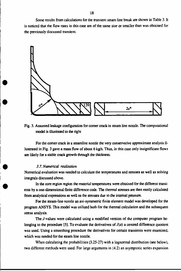
Some results from calculations for the transient steam line break are shown in Table 3. It

is noticed that the flow rates in this case are of the same size or smaller than was obtained for

the previously discussed transient.

2a*

Fig. 3. Assumed leakage configuration for corner crack in steam line nozzle. The computational

model is illustrated to the right

For the corner crack in a steamline nozzle the very conservative approximate analysis il-

lustrated in Fig. 3 gave a mass flow of about 6 kg/s. Thus, in this case only insignificant flows

are likely for a stable crack growth through the thickness.

3.7. Numerical realization

Numerical evaluation was needed to calculate the temperatures and stresses as well as solving

integrals discussed above.

In the core region region the material temperatures were obtained for the different transi-

ents by a one-dimensional finite difference code. The thermal stresses are then easily calculated

from analytical expressions as well as the stresses due to the internal pressure.

For the steam-line nozzle an axi-symmetric finite element model was developed for the

program ANSYS. This model was utilized both for the thermal calculation and the subsequent

stress analysis.

The /-values were calculated using a modified version of the computer program be-

longing to the procedure [5]. To evaluate the derivatives of J(a) a centred difference quotient

was used. Using a smoothing procedure the derivatives for certain transients were examined,

which was needed for the steam line nozzle.

When calculating the probabilities (3.25-27) with a lognormal distribution (see below),

two different methods were used. For large arguments in (4.2) an asymptotic series expansion

19

of the erfc-function was used. For small arguments a Chebyshev fitting of the erfc-function

was found satisfactory. Last, when calculating the probabilities (3.28-29) for preservice

defects, the probability density function given in discrete points was fitted to a multilinear

function. The integration was performed by a modified Romberg integration scheme.

4. Input data

4.1. Stress distributions

The different categories uf stress considered in the two regions are summarized in table 4.

Loading

Thermal stress

Pressure stress

Residual stress

core region

primary stress

X

-

secondary stress

X

-

X

steam line nozzle

primary stress

-

X

(membrane)

-

secondary stress

X

X

(bending)

-

Table 4. Categorization of stress in different regions.

The pressure and thermal stresses were calculated as described above while the residual stress

level in the core was chosen according to the guidelines in [5]. An example of a typical calcu-

lated stress distribution is shown in Fig. 4.

£

V)Vi

I

t= 300 s

t=9OOs

t=18OOs

-100 -

-2000.02 0.04 0.06 0.08 0.1 0.12

distance from inner wall [m]0.14

Fig. 4. Stress distribution in the core region due to a steam line break.

20

42. Fracture toughness properties

Fairly little information is available for the random distribution of fracture toughness and related

properties. In the lower shelf and transition region Wallin [IS] and others have argued for the

use of Weibull type distributions. In the absence of a minimum fracture toughness level the dis-

tribution proposed in [15] takes the form

FJo(J) = 1 - exp4/2

(4.1)

where 7 o is the mean value of Jo . We here use this distribution for temperatures below To.

The mean value is chosen to correspond to the upper shelf level of the ASME curve and thus

7 o =0.25 MN/m.

In the wholly ductile temperature region eq. (4.1) is not considered appropriate. The re-

sults in [16] instead suggest a lognormal distribution viz.

FJo(J) = 0.5(4.2)

Here erf denotes the error function and the parameters my and Sj are related to J o and the

standard deviation o> of Jo according to

7 o = exp (my + sj2/2) ,

<r, = 7 0 [exp(,y2)-l]1/2.

(4.3)

(4.4)

From the results of [16] the parameters m} and sf were estimated to -1.414 and 0.225 at the

temperature 270 °C. These data were rescaled so that the mean 7 o coincides with the value

0.25 MN/m which is the upper shelf level of the ASME curve. The standard deviation was

scaled proportionally so that 07 = 0.228 J 0. The lognormal distribution with these parameter

values is in the following termed lognormal 1.

Distribution

Weibull

Lognormal 1

Lognormal 2

Mean value

[MN/m]

0.25

0.25

0.25

Standard deviation

[MN/m]

0.0951

0.0569

0.112

Table 5. Properties of assumed fracture toughness distributions

21

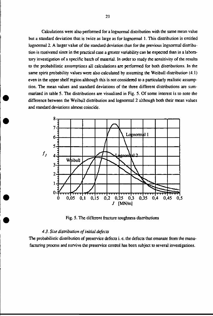
Calculations were also performed for a lognormal distribution with the same mean value

but a standard deviation that is twice as large as for lognormal 1. This distribution is entitled

lognormal 2. A larger value of the standard deviation than for the previous lognormal distribu-

tion is motivated since in the practical case a greater variability can be expected than in a labora-

tory investigation of a specific batch of material. In order to study the sensitivity of the results

to the probabilistic assumptions all calculations are performed for both distributions. In the

same spirit probability values were also calculated by assuming the Weibull distribution (4.1)

even in the upper shelf region although this is not considered to a particularly realistic assump-

tion. The mean values and standard deviations of the three different distributions are sum-

marized in table 5. The distributions are visualized in Fig. 5. Of some interest is to note the

difference between the Weibull distribution and lognormal 2 although both their mean values

and standard deviations almost coincide.

8

fj: W

i /!/

- i i i i1

»bully

/ //

f

T/

\ Lo

\

\

\

;norm

al 2

\

\

ill

0 0,05 0,1 0,15 0,2 0,25 0,3 0,35 0,4 0,45 0,5J [MN/m]

Fig. 5. The different fracture toughness distributions

4.3. Size distribution of initial defects

The probabilistic distribution of preservice defects i. e. the defects that emanate from the manu-

facturing process and survive the preservice control has been subject to several investigations.

22

lxlO3-

i IA2-

lxlO1-

lxlO1-

i m-3^

lxlO"4-

V

\

\

\

^ \

O 0,025 0,05 0,075a [m]

0,1 0,125 0,15

Fig. 6. The OCTAVIA-distribution

A good summary of the efforts up to 1986 can be found in [3]. Three different distribution

types have been used more frequently. The first is the distribution developed in the Marshall re-

port [2], the second the so-called OCTAVIA distribution (cf. [3]) and the third a distribution

developed by Dufresne and Lucia [17]. Of these, the OCTAVIA distribution is the middle one

with respect to conservatism with the Marshall distribution as the more conservative one and the

Dufresne distribution as the less conservative one. For this study it was considered appropriate

to use the OCTAVIA distribution which is visualized in Fig. 6.

The length distribution of the cracks may also be of some interest for calculation of lea-

kage rates. As pointed out below the calculations show that it is very unlikely that leakage

occurs before break so no efforts were spent on establishing a length distribution function.

4.4. Crack growth calculations

Fatigue crack growth is limited in most pans of the reactor vessel and conventional methods for

calculating this growth were sufficient. In all cases a fatigue crack growth law according to

ASME Sect. XI [1] was assumed.

dadN

AK,

AK0(R)10"6 [m/cycle]. (4.5)

Here AK0 and n are material constants depending on the stress ratio R.

23

In the core region (region I) the dominating stress cycle is the start up-loss of power

shut down cycle. Consideration of the residual stress gives that 0.25<fl<0.65 and from [1]

n=1.95 together with AK0=17.7 MPam1/2. The resulting calculations show that

0.048S A^floo < 0.065, 0.07 £ a^Jd < 0.72. (4.6)

The crack growth increment A5C is thus limited and for simplicity it is set to 0.06OQ.

For the corner crack (region II) the fatigue crack growth data are slightly different from

those of the core region since no residual stress is assumed to be present and thus the lvalue is

lower. The material parameter AAT0 becomes 13.3 MPam1/2 while n remains the same. For this

case we obtain

0.06< A^aoo £ 0.096, 0.036 < a^Jd < 1.44. (4.6)

The crack growth increment A,c is set to O.O95ao.

Data about stress corrosion cracking are scarce and seem to be somewhat controversial.

Speidel and Magdowski [18] report growth rates of the order 10'8 m/s in an environment with

stagnant flow and high sulphur concentration. According to several assessments this high a rate

is not considered relevant to conditions in Swedish BWRs. Instead a growth rate of 2 10"10 m/s

was used as a reference value. This was suggested by in [18] as appropriate for normal BWR

environments and the growth rate is approximately independent of the stress intensity factor.

According to the same article the threshold value should be in the interval 10 <Khscc< 30

MPam1/2. This means that a crack penetrating the cladding in most cases will have a Kj value

that exceeds the threshold value. The growth rate 210*10 m/s means that the crack will grow 63

mm during ten years and this value has been assumed for the basic set of calculations.

45. Crack incidence rates

Very little information exist about the crack incidence rates both for preservice defects and for

inservice defects. A common assumption used in previous probabilistic investigations is to as-

sume that there exists on average one significant preservice defect per reactor vessel and then

simply assume that the occurrence rates in different regions is proportional to the weld volume

in each region.

The type of inservice defects that are of main concern here namely stress corrosion

cracking has to the knowledge of the authors only occurred once in a reactor pressure vessel.

This was in the Quad City unit where ISC was detected in 1990. A number of circumferentially

oriented cracks were detected of which the largest one was 760 mm long.

The total number of service years of BWRs is presently 981 years in the world. A sim-

ple estimate of the occurrence rate would thus giving be 10'3 per reactor and year. In a ten year

period the probability of occurrence is then 10'2 for the entire vessel.

24

5. Results5.7. Basic set of indata

Calculations were performed to obtained the auxiliary quantities J^ etc. defined above for the

different regions and loading conditions. These calculations gave widely different results for

different load cases. One example of a relatively smooth variation of JOin is shown in Fig. 7

which is for the core region and the load case turbine trip. JOut and J^ at the time 300 s are

shown in the figure. We note that these quantities are fairly close to each other which means

that the probability of stable growth though the thickness will become very small. The resulting

probabilities are drawn as function of crack depth in Fig. 8. It is noted that the probability of a

stable growth through the thickness is zero for crack depths less than 0.1 m due to the pre-

viously mentioned reasons.

An example of a much more irregular situation is shown in Fig. 9 where the JOm and

JOst values for a comer crack in the steam line nozzle for the case level increase are drawn.

Clearly, the corresponding probabilities will display a very irregular behaviour in this case

which is difficult to visualize in a figure.

0,1-

0,075-

0,05-

0,025-

0-

•

•

•

fl

a

\ ^ ^ ~

/JIn

0 0,05aQ[m]

0,1 0,15

Fig. 7. JQiH and JQ,, at time 300 s as functions of crack depth for turbine trip, core region.

The resulting values of the fracture and leakage probabilities when the crack size distribution

and crack growth have been taken into account are documented in the Appendix. It is noted

from the tables that the fracture toughness distribution has a large effect The Weibull distribu-

tion is the most conservative and lognormal 1 the least conservative. According to the previous

discussion the Weibull distribution is probably not very relevant for the events in the upper

shelf region and in this regime the lognormal distributions are believed to be the more represen-

tative.

25

.O-

1O3

1O4

pst

106

107

108

109

l o io

0,05 0,1 0,co[m]

15 0

1

4

1

WeibullJ

ocnormal 1

n\\\ \

\ \\ \

0,15

Fig. 8. Pin and Psl at time 300 s as functions of crack depth for turbine trip, core region.

0,001

0,00075

0.0005

0,00025-

öo[m]

Fig. 9. /aVl and JQ,, at time s as functions of crack radius for level increase, steam line nozzle.

It is seen for the core region that the COP is the most dangerous event. The difference

between the three toughness distributions is not as marked as for the remaining load cases. In

the nozzle region the COP event is less dangerous due to the lower transition temperature in this

region and is in fact about as detrimental as the reactor isolation transient. The COP event requi-

res somewhat special attention since it will almost certainly cause failure in the core region if

there is any inservice defect at all.

With access to the basic fracture and leakage probabilities in Table Al and A2 it is an

easy matter to obtain the final probabilities simply by performing the multiplications implied in

26

eqs. (2.1).and (2.2). In table 6 the incidence rates for preservice and inservice defects as well

as the load case probability have been accounted for. The contributions due to preservice and

inservice defects, respectively, have been summed. In the table the largest probability with

respect to load case (excepting the COP event because the special impact this event has in the

core region) has been bolded

Region

Core

region

Corner

crack in

steam

line

nozzle

Load case

TT

RI

SLB

COP

RI

U

SLB

COP

Event

Fracture

Leakage

Fracture

Leakage

Fracture

Leakage

Fracture

Leakage

Fracture

Leakage

Fracture

Leakage

Fracture

Leakage

Fracture

Leakage

Weibull

4.7310-5

2 . 6 5 1 0 9

6 . 8 1 1 0 s

0.

2.06-10-7

9.991013

1.0810"7

0.

2 .52-10 4

1.6410"4

8.91 10'5

6.1110'5

8.6510"8

5.95108

1.6110"9

1.0710"9

Lognormal 1

1.191012

2 . 4 3 1 0 1 2

6 . 9 M 0 1 1

0.

9.66-1019

7.68-10-20

1.0110-7

0.

1.8310"9

7.03-1018

4.85-1010

4 . 1 0 1 0 1 6

4.66-1013

3.24-10"23

1.12101 4

8.31-10'20

Lognormal 2

2.80-10-9

1 . 1 3 1 0 ' 9

7 . 5 4 - 1 0 "

0.

5.96-1012

7.14-1014

i.oo-io-7

0.

9 . 0 1 1 0 - 7

1 . 1 8 1 0 7

5.12-10"9

4.9 M O 1 0

4 .4110 1 2

4 .1910 1 3

1.09101 2

1.27-1013

Table 6. Fracture and leakage probabilities per region and load case.

5.2. Some sensitivity studies

In order to to study the sensitivity of the results to different assumptions about the input data a

limited sensitivity study was carried out.

The COP event gave very large fracture probabilities in the core region. Obviously the

risk of fracture will be dependent of the transition temperature of the material. In the basic set of

data RTNDT has been assumed to be 33 °C in the core region and -15 °C for the steam line

nozzle. In Fig. 10 and 11 the fracture probabilities due to a preservice defect and an inservice

defect, respectively, are shown as function of RTNDT. As can be seen the fracture probabilities

decrease dramatically with decreasing RTNDT .The interpretation is that the risk due to a COP

event is negligible if the transition temperature is below 0 °C. This in turn means that the

importance of the COP event will vary considerably between different reactor vessels.

27

-10

RTN

TNDT

Fig. 10. PfiP as function of RTNar for a preservice defect for a COP event

10°

101

io-2

10"3

io-5

io-6

WeibuU L - ^ 5

A?/ /ULognonaal2

/l/ I Lognorm

/ 1

i l l

-10 0 10 20

RT

30 40 50

Fig. 11. Pfk

ti as 'unction of RTNm for a inservice defect for a COP event.

As mentioned above the stress corrosion cracking rate is also fairly uncertain. The influ-

ence of the rate was studied by considering the core region for the loading case reactor isola-

tion. In Fig. 12 the result for the failure probability is shown. Again a fairly dramatic depend-

ence on the growth rate is observed.

28

pk

fei

10-5-

10-10.

1 015-

10-20.

weiDuii— •

sy

s

-~

Lopnormai J. ^

— = = - -

^ /^ /

//

//

Lopnormai 1 //

//

//

//

*0,010° 1,0 10 10 2 . 0 1 0 1 0

growth rate [m/s]

3.0 1 0 1 0

Fig. 12. as function of the stress corrosion cracking rate for an inservice defect.

6. Discussion

It is noticed from table 6 that the fracture toughness distribution has a very dramatic effect on

the resulting fracture and leakage probabilities. In fact this influence is so large that any absolute

interpretation of the probabilities is meaningless except for the high risk cases. Even for the

Weibull and the lognormal 2 distributions which have nearly the same standard deviations the

resulting probabilities differ considerably illuminating the sensitivity to the tail behaviour earlier

noted by Palm and Nilsson [19]. It is, however, observed that the ranking of the two geomet-

ries is mainly the same regardless of which fracture toughness distribution that is chosen. If the

range of probabilities obtained is taken as a measure of the uncertainty we note that for a crack

in the core region the factor between the fracture probability for the two lognormal distributions

is of order 102 (again excepting the COP event). The corresponding number for the corner

crack roughly of the same order. In both cases the RI transient is the dominating one. The

difference between the two regions is also about a factor of 102 and thus seems to be signifi-

cant

Another observation of interest is that the probabilities of leakage are in general much

smaller than the ones for fracture. This has the consequence that the probability of leakage in

the categories large and moderate is insignificant. This in tum suggest that consequence aspects

are not especially important when allocating in-service inspection efforts.

When judging the results of the investigation it has to be kept in mind that relatively

crude fracture mechanics models have been used and extrapolation beyond validity limits has

occasionally been necessary.

29

7. Conclusions

- The results obtained so far do seem to indicate that a differentiation between regions based on

probabilistic fracture mechanics is viable.

- The COP event dominates the failure probability of the core region if the rate of occurrence is

as assumed. If the COP is excepted the RI transient is the dominating risk contributor.

- Consequence considerations do not seem to be of importance for differentiation between the

different regions.

AcknowledgementThis work was funded by the Swedish Nuclear Power Inspectorate. The authors want to ex-

press their gratitude for this support. We also appreciate the discussions with Drs. G. Hedner,

L. Dahlberg and Mr. T. Andersson.

30

References

[1] American Society of Mechanical Engineers Boiler and Pressure Vessel Code, Section

XI: Inservice inspection.

[2] Marshall, W., "An assessment of the integrity ofPWR pressure vessels", Study Group

Report, Services Branch, United Kingdom Atomic Energy Agency, London, 1976.

[3] Simonen, F. A., Johnson, K. J., Liebetrau, A. M., Engel, D. W. and Simonen, E. P.,

"VISA-II -A computer code for predicting the probability of reactor pressure vessel

failure", NUREG/CR-4486, PNL-5775, USNRC, 1986.

[4] Milne, I., Ainsworth, R. A., Dowling, A. R. and Stewart, A. T., "Assessment of the

integrity of structures containing defects" ,CEGB Report R/H/R6-Rev. 3, Central

Electricity Generating Board, 1988.

[5] Bergman, M , Brickstad, B., Dahlberg, L., Sattari-Far, I. and Nilsson, F., "A

procedure for safety assessment of components with cracks", SA/FoU Repon 91/01,

The Swedish Plant Inspectorate, Stockholm, 1991.

[6] Nilsson, F., Faleskog, J., Zarcmba, K. and Öberg, H., "Elastic-plastic fracture

mechanics for pressure vessel design", to appear in Fatigue and Fracture of Engi-

neering Materials and Structures, 1991.

[7] Östensson, B., "Experimentell undersökning av brottsegheten hos tryckkärlsstål A-533

B i temperaturintervallet 20 °C - 350 °C", report S-509, AB Atomenergi, Studsvik,

1975.

[8] Nilsson, F., "Reliability assessment by aid of probabilistic fracture mechanics", OECD/

NEA/CSNI Workshop on Safety Assessment of Reactor Pressure Vessels, VTT, Esbo,

1990.

[9] Raju, I. S. and Newman, J. C , "Stress-intensity factor influence coefficients for

internal and external surface cracks in reactor vessels", Mechanics of Crack Growth,

ASTMSTP 590, ASTM, Philadelphia, 37-48, 1978.

[10] Harrison, R. P., Loosemore, K., Milne, I., and Dowling, A. R., "Assessment of the

integrity of structures containing defects" ,CEGB Repon R/H/R6-Rev. 2, Central

Electricity Generating Board, 1980.

31

[11] Sattari-Far, I. and Nilsson, F., "Validation of a procedure for safety assessment of

cracks", SA FoUReport 90/04,1990.

[12] Kobayashi, A. S and Enetanya, A. N., "Stress intensity factor of a corner crack",

Mechanics of Crack Growth, ASTM STP 590, ASTM, Philadelphia, 477-495, 1978.

[13] Miller, A. G., "Elastic crack opening displacements and rotations in through-cracks in

spheres and cylinders under membrane and bending loading", Eng. Fract. Mech, 23,

631-648, 1986.

[14] Langston, D. B., Haines, N. F. and Wilson, R., "Development of a leak-before break

procedure for pressurized components", Proceedings Tenth International Conference on

Structural Mechanics in Reactor Technology, ed. by A. H. Hadjian, vol. G, 287-291,

1989.

[15] Wallin, K, "The size effect in KIc results", Eng. Fract. Mech., 22, pp.149-163,1985.

[16] Nilsson, F. and Östensson, B., "Jlc- testing of A-533 B - statistical evaluation of some

different testing techniques", Eng. Fract. Mech., 10,1978,223-232.

[ 17] Dufresne, J. and Lucia A., "A probabilistic approach to the evaluation of pressure

vessels safety margins," in Structural Integrity of Light Water Reactor Components, ed.

Steel, L. E., Stahlkopf, K. E. and Larsson, L. H., Applied Science Publishers,

London and New York, 1981.

[ 18] Speidel, M. O. and Magdowski, R. M., "Stress corrosion cracking of nuclear reactor

pressure vessels and piping", Int. J. Pres. Vessels and Piping, 34,1988,119-142.

[19] Palm, S. and Nilsson, F. "Sensitivity analysis of the failure probability of a reactor

pressure vessel", in Current Nuclear Power Plant Safety Issues, II, International

Atomic Energy Agency, IAEA-CN-39/80,1981,365-381.

32

Appendix, basic fracture and leakage probabilities

Load case

Turbine trip

(TT)

Reactor

isolation (RI)

Steam-line

break (SLB)

Cold over-

pressurization

during outage

(COP)

Probability

Fracture, pre, Pfk

tB

Fracture, in, Pfk

ti

Leakage, pre, Pup

Leakage, in, Pkti

Fracture, pre, Pfk

0

Fracture, in, P(k,

Leakage, pre, Pkep

Leakage, in, P,kei

Fracture, pre, Pfk,o

Fracture, in, Pfk,

Leakage, pre, Pkep

Leakage, in, Pkt>

Fracture, pre, PktD

Fracture, in, />,*•

Leakage, pre, Pkt0

Leakage, in, /?*,

WeibuU

6.59-10-5

4.07-10"3

2.65-10"8

0.

3.4 HO"5

6.47-103

0.

0.

1.1410'3

9 . 2 1 1 0 3

9.99-10"9

0.

8 .0410 3

0.998

0.

0.

Lognormal 1

1.1910 1 1

3.25 10-31

2 .4310 1 1

0.

6 . 9 1 1 0 1 0

3.1410"26

0.

0.

9 . 6 6 1 0 1 5

1.0010"22

7 . 6 8 1 0 1 6

0.

5.2110"4

1.00

0.

0.

Lognormal 2 |

2.76-10"8

3.73-10"9

1.1310 8

0.

6.84-10-8

7.0110-8

0.

0.

4.05-10"9

5.5610-7

7 .1410 1 0

0.

1.0910 3

0.991

0.

0.

Table Al. Basic fracture and leakage probabilities for the core region.

33

Load case

Reactor

isolation (RI)

Level increase

during shut-

down (LI)

Steam-line

break (SLB)

Cold over-

pressurization

during outage

(COP)

Probability

Fracture, pre, Pfktp

Fracture, in, Pfkti

Leakage, pre, Pktp

Leakage, in, P,kei

Fracture, pre, Pfktp

Fracture, in, Pfkti

Leakage, pre, Pktp

Leakage, in, / &

Fracture, pre, Pktp

Fracture, in, /}*,

Leakage, pre, Pktp

Leakage, in, Pkei

Fracture, pre, Pktp

Fracture, in, /»,*•

Leakage, pre, PktP

Leakage, in, JJ*-

WeibuU

2.74-10-4

2.5 MO"2

4.49-10'6

1.6410-2

1.3710"4

8 .8910 3

1.99 10-6

6.1 MO"3

1.34 lO"4

8.64-103

1.9510 6

5.9510"3

1.4510-4

1.6110-2

2.47-10"6

1.07-IQ"2

Lognormal 1

1.8310"6

3 .4010 1 4

6 .8910 1 5

1.4010 1 7

4.85-10-7

4.60-1O"23

4 .1010 1 3

8.22-10-27

4.66-lO"7

2.43-10-23

3 .2410 1 7

4.23-lO27

1.1210"6

9 .8410 1 8

8 .3110 1 2

2.47-10-21

Lognormal2

2.2510"6

8.99-10-5

4 . 2 5 1 0 1 0

1.1810"5

5.72-10"7

4.55-107

2.14-1012

4.97-10-*

5.49-10-7

3.86-10"7

1.5710 1 2

4 . 1 9 1 0 8

1.57-106

1.O81O5

4.34-1011

1.2710"6

Table A2. Basic fracture and leakage probabilities for a comer crack in the steam line nozzle.