application of remote sensing and gis in · pdf fileapplication of remote sensing and gis in...
TRANSCRIPT

APPLICATION OF REMOTE SENSING AND GIS IN URBAN LAND SUITABILITY MODELING AT PARCEL LEVEL USING
MULTI-CRITERIA DECISION ANALYSIS
Thesis submitted to the Andhra University, Visakhapatnam in partial fulfillment of the requirements for the award of
Master of Technology in Remote Sensing & Geographic Information System
by
M Raghunath, Senior Grade Lecturer, SJ(Govt.) Polytechnic,
Bangalore
Internal Supervisor Mr. Sandeep Maithani Scientist-SE, HUSAG,
IIRS, DehraDun
External Supervisor Dr. H.Honnegowda, Director, KSRSAC,
Bangalore
iirs Indian Institute of Remote Sensing
National Remote Sensing Agency Dept. of Space, Govt. of India
Debra Dun-248 001 INDIA
2006

Application of RS & GIS for Urban Land Suitability Modeling at Parcel Level using MCDA 2
Chapter No. Description Page No.
Certificates i
Acknowledgement iii
List of Maps and Diagrams iv
List of Tables vii
1 Introduction 1-1
2 Cadastral Maps 2-1
3 Basic Concepts of Remote Sensing and GIS 3-1
4 Multi-Criteria Data Analysis 4-1
5 Urban Land Suitability Evaluation 5-1
6 Study Area – Bangalore 6-1
7 Methodology and Database Creation 7-1
8 Analysis and results 8-1
9 Summary and Conclusion 9-1
Appendix-A A-1
Bibliography B-1

Application of RS & GIS for Urban Land Suitability Modeling at Parcel Level using MCDA 3
Karnataka State Remote Sensing Application Center,
6th Floor, Multi-Storeyed Buildings, Vidhana Veedhi,
Bangalore – 560 001, Karnataka (State), INDIA
CERTIFICATECERTIFICATECERTIFICATECERTIFICATE
This is to certify that Sri. M. Raghunath, Senior Grade Lecturer in Civil
Engineering, S.J.(Govt.) Polytechnic, Bangalore, has carried out the project
entitled “ Application of Remote Sensing and GIS for Urban Land Suitability
Modeling at Parcel Level using Multi-Criteria Decision Analysis (MCDA) “ as a
partial fulfillment for the award of M.Tech(RS&GIS) degree in stream of ‘Urban
and Regional Planning’ by Andra University at the Karnataka State Remote
Sensing and Applications Center, Bangalore.
The report contains original work carried by the trainee and has used the
available data at this center.
(Dr. H . Honne Gowda)
External Guide &
Director, KSRSAC
Bangalore

Application of RS & GIS for Urban Land Suitability Modeling at Parcel Level using MCDA 4
Indian Institute of Indian Institute of Indian Institute of Indian Institute of Remote SensingRemote SensingRemote SensingRemote Sensing
(National Remote Sensing Agency)(National Remote Sensing Agency)(National Remote Sensing Agency)(National Remote Sensing Agency)
(Dept. of Space, Govt. of India)(Dept. of Space, Govt. of India)(Dept. of Space, Govt. of India)(Dept. of Space, Govt. of India)
Kalidas Road, PB No: 135, Kalidas Road, PB No: 135, Kalidas Road, PB No: 135, Kalidas Road, PB No: 135,
DEHARADUN DEHARADUN DEHARADUN DEHARADUN –––– 248 001 (INDIA) 248 001 (INDIA) 248 001 (INDIA) 248 001 (INDIA)
CERTIFICTECERTIFICTECERTIFICTECERTIFICTE
This is to certify that Sri. M. RaghunathM. RaghunathM. RaghunathM. Raghunath, Senior Grade Lecturer in Civil
Engineering, S.J.(Govt.) Polytechnic, Bangalore has carried out the project
entitled “ Application of Remote Sensing and GIS for Urban Land Suitability “ Application of Remote Sensing and GIS for Urban Land Suitability “ Application of Remote Sensing and GIS for Urban Land Suitability “ Application of Remote Sensing and GIS for Urban Land Suitability
Modeling at Parcel Level using MultiModeling at Parcel Level using MultiModeling at Parcel Level using MultiModeling at Parcel Level using Multi----Criteria Decision Analysis (MCDA) “Criteria Decision Analysis (MCDA) “Criteria Decision Analysis (MCDA) “Criteria Decision Analysis (MCDA) “ as a
partial fulfillment for the award of M.Tech(RS&GIS)M.Tech(RS&GIS)M.Tech(RS&GIS)M.Tech(RS&GIS) degree in stream of ‘Urban Urban Urban Urban
and Regional Planningand Regional Planningand Regional Planningand Regional Planning’’’’ of Andra UniversityAndra UniversityAndra UniversityAndra University at the Karnataka State Remote Karnataka State Remote Karnataka State Remote Karnataka State Remote
Sensing and Applications Center (KSRSAC)Sensing and Applications Center (KSRSAC)Sensing and Applications Center (KSRSAC)Sensing and Applications Center (KSRSAC), Bangalore.
The report contains original work carried by the trainee and has duly
acknowledged the data sources and the facilities used by him.
(Mr. Sandeep Maithani) (Mr. Sandeep Maithani) (Mr. Sandeep Maithani) (Mr. Sandeep Maithani) (Mr. B.S.Sokhi)(Mr. B.S.Sokhi)(Mr. B.S.Sokhi)(Mr. B.S.Sokhi)
Internal Project Guide Head, HUSAG, IIRS
Scientist, HUSAG, IIRS Dehardun
Dehradun
(Dr. V.K. Dadhwal)(Dr. V.K. Dadhwal)(Dr. V.K. Dadhwal)(Dr. V.K. Dadhwal)
Dean, IIRS
Dehradun

Application of RS & GIS for Urban Land Suitability Modeling at Parcel Level using MCDA 5
ACKNOWLEDGEMENT
It gives me immense pleasure to express my sincere appreciation of the
assistance rendered to me by all those who helped me in completing this
project. At the outset I express my deep sense of gratitude to the Prof.Prof.Prof.Prof.
BasavarajBasavarajBasavarajBasavaraj, Director, Department of Technical Education, Government of
Karnataka, Bangalore, for deputing me to undergo M.Tech(RS&GIS) Degree
program at Indian Institute of Remote Sensing, NRSA, Department of Space,
Dehradun. I express my heartfelt gratitude to Mr. P.S. RoyMr. P.S. RoyMr. P.S. RoyMr. P.S. Roy, the former Dean who
opened the gateway for M.Tech (RS&GIS) program and selected me to undergo
this course. Also I thank Dr.V.K. DadhwalDr.V.K. DadhwalDr.V.K. DadhwalDr.V.K. Dadhwal, the present Dean who permitted me
to do my project work at KSRSAC, Bangalore.
I sincerely thank Mr.Mr.Mr.Mr. GovilGovilGovilGovil, Head, Photogrammetry and remote Sensing
(PRS) Division and also the faculty members of PRS Division, who helped me to
understand the science and technology of RS&GIS.
Also, I sincerely express my gratitude to Mr. B.S.SokhiMr. B.S.SokhiMr. B.S.SokhiMr. B.S.Sokhi, Head, Human and
Urban Settlement Analysis Group (HUSAG), for his valuable guidance,
cooperation and suggestions. Nevertheless, I thank Mr. Sandeep MaithaniMr. Sandeep MaithaniMr. Sandeep MaithaniMr. Sandeep Maithani,
Scientist, who helped and spent long hours with me, day and night, during my
short stay at IIRS, Dehradun. Also I thank Miss. Sadhana Jain, Scientist, and Dr.
Bharath, Scientist, in HUSAG for their valuable guidance and cooperation during
the course of study.
I would like to express my deepest gratitude to Dr.H. HonnegowdaDr.H. HonnegowdaDr.H. HonnegowdaDr.H. Honnegowda,
Director, Karnataka State Remote Sensing Applications Center, Department of
IT&BT, Govt. of Karnataka, Bangalore for granting permission to carry out my
project work at his premises and extending his fullest support by providing
proper guidance, suggestions, Quick Bird Satellite data, the cadastral maps, the
hardware and software and above all available soil and ground water prospects
data for my study area. I do not find suitable words to express my thanks to the
staff of KSRSAC who shared their experiences and helped me to learn the
practical aspects of RS and GIS.
Last but not the least, I put on record the encouragement, cooperation
and selfless sacrifice, during my stay away from home, of my wife Y.S.Veena
and my little daughter R. Sanjana, which lead me to successfully complete this
project work.
Bangalore M. Raghunath

Application of RS & GIS for Urban Land Suitability Modeling at Parcel Level using MCDA 6
List of Maps and DiagramsList of Maps and DiagramsList of Maps and DiagramsList of Maps and Diagrams
Figure 1.1: Unstructured and structured problems
Figure 2.1: A typical Cadastral Map (Gunjur Village, Bangalore Urban South Tq.)
Figure 2.2: Legend for Cadastral Maps
Figure 3.1: Energy interactions in the atmosphere
Figure 3.2: Stages in Remote Sensing process
Figure 3.3: Passive sensors
Figure 3.4: Active Sensors
Figure 3.5: Ground, Air and Space Borne Remote Sensing
Figure 3.6: Satellite orbits
Figure 3.7: Various data input devices/methods
Figure 3.8: Components of GIS
Figure 3.9: GIS Thematic layers representing real world features
Figure 3.10: Representation of the real world and showing differences in how a
vector and a raster GIS will represent this real world.
Figure 3.11: Vector data format
Figure 3.12: Raster data format
Figure 4.1: Relationship among the elements of MCDA
Figure 4.2: Framework of Spatial Multi-criteria Decision Analysis
Figure 6.1: Location map of Bangalore City
Figure 6.2: Study area over topographic sheet mosaic of Bangalore
Figure 6.3: Location Of Study Area Over Master Plan
Figure 6.4 Location Of Study Area Over BDA Administrative area
Figure 6.5: Population distribution in BMP wards
Figure 7.1: Methodology of Creating Urban Suitability Map at Parcel Level
Figure 7.2: Subset Study Area of Quick Bird Merged Image
Figure 7.3: Existing Manually Digitized Landuse/landcover Map

Application of RS & GIS for Urban Land Suitability Modeling at Parcel Level using MCDA 7
Figure 7.4: Ground Water Prospects Map
Figure 7.5: Soil Depth Map
Figure 7.6: Soil Texture Map
Figure 7.7: Land Value(Government) Map
Figure 7.8: Proximity to Road Network Map
Figure 7.9: Proximity to Built-up Area Map
Figure 7.10: Master Plan Constraint Map
Figure 7.11: Built-up Area Constraint Map
Figure 7.12: Water Bodies Constraint Map
Figure 7.13: Overlay of Geo-referenced Cadastral Map of Gunjur Village over
Quick Bird Merged Image
Figure 7.14: Overlay of Geo-referenced Cadastral Vector Parcel Layer over
Quick Bird Image
Figure 7.15: Village wise Parcel Vector Layer
Figure 7.16: Overlay of Cadastral Vector Parcel Layer over Quick Bird Image
Figure 8.1: Graph showing the comparison of areas of Urban Land Suitability
classes of different models.
Figure 8.2: Graph showing the comparison of areas of different Urban land
suitability classes of all models for Gunjur village
Figure 8.3: Pie Chart Showing the Percentage of Areas of Different Urban Land
Suitability Classes of Parcel No 303 – Models 1&2
Figure 8.4: Pie Chart Showing the Percentage of Areas of Different Urban Land
Suitability Classes of Parcel No 303 – Model -3
Figure 8.5: Pie Chart Showing the Percentage of Areas of Different Urban Land
Suitability Classes of Parcel No 303 – Model-4
Figure 8.6: Urban land Suitability Map For Urban Suitability Model 1
Figure 8.7: Urban land Suitability Map For Urban Suitability Model 2

Application of RS & GIS for Urban Land Suitability Modeling at Parcel Level using MCDA 8
Figure 8.8: Urban land Suitability Map For Urban Suitability Model 3
Figure 8.9: Urban land Suitability Map For Urban Suitability Model 4
Figure 8.10: Parcel Level Urban Land Suitability Map for Model – 1
Figure 8.11: Parcel Level Urban Land Suitability Map for Model – 2
Figure 8.12: Parcel Level Urban Land Suitability Map for Model – 3
Figure 8.13: Parcel Level Urban Land Suitability Map for Model – 4
Figure 8.14: Gunjur Village Parcel Level urban land suitability map: model-1
Figure 8.15: Gunjur Village Parcel Level urban land suitability map: model-2
Figure 8.16: Gunjur Village Parcel Level urban land suitability map: model-3
Figure 8.17: Gunjur Village Parcel Level urban land suitability map: model-4
Figure 8.18: Gunjur Village Parcel Level urban land suitability map for Parcel
No: 303 : model-1
Figure 8.19: Gunjur Village Parcel Level urban land suitability map for Parcel
No: 303 : model-2
Figure 8.20: Gunjur Village Parcel Level urban land suitability map for Parcel
No: 303 : model-3
Figure 8.21: Gunjur Village Parcel Level urban land suitability map for Parcel
No: 303 : model-4

Application of RS & GIS for Urban Land Suitability Modeling at Parcel Level using MCDA 9
List of Tables:List of Tables:List of Tables:List of Tables:
Table 1.1: Percentage of urban population and its contribution to national
income
Table 1.2: Specifications of Quick Bird satellite
Table 1.3: SOI maps
Table 1.4: Villages and their extent in Hectares in the Study Area
Table 3.1: Satellite Imagery for Different Levels of Development Planning
Table 3.2: Operational Satellites
Table 4.1: Comparison of MODM and MADM
Table 5.1: List of physical parameters and their importance in land suitability
for urban development
Table 5.2: Sources of data
Table 6.1: Rainfall in Bangalore Urban District
Table 6.2: Population of Bangalore from 1950 to 2015
Table 6.3: Ward / CMC- wise Population as per census 2001
Table 7.1 : Areas of Landuse/Landcover Classes in the study area
Table 7.2 : Areas of Ground Water prospects Classes in the study area
Table 7.3 : Areas of Soil Depth Classes in the study area
Table 7.4 : Areas of Soil Texture Classes in the study area
Table 7.5 : Areas of Land Value Classes in the study area
Table 7.6 : Areas of Proximity to Road Classes in the study area
Table 7.7 : Areas of Proximity to Built-up Classes in the study area
Table 7.8 : Areas of Constraint (Master Plan) Classes in the study area
Table 7.9 : Areas of Constraint(Built-up) Classes in the study area
Table 7.10: Areas of Constraint(Water Body) Classes in the study area
Table 8.1 : Saaty’s scale of importance
Table 8.2: Importance matrix for Model-1

Application of RS & GIS for Urban Land Suitability Modeling at Parcel Level using MCDA 10
Table 8.3: Importance matrix for Model-2
Table 8.4: Importance matrix for Model-3
Table 8.5: Importance matrix for Model-4
Table 8.6: Weightage derived from the Saaty’s AHP method:
Table 8.7: Ranking System For The Categories Of The Factors/Parameters
Table 8.8: Comparative Gross Areas of Suitability Classes of Different Models
Table 8.9: Village-wise Comparative Areas of Different Land Suitability
Classes and models
Table 8.10: Example showing Gunjur Village Multi-Suitability Class Affiliation of
Same Parcel To different classes : Model - 1
Table 8.11 :Example showing Gunjur Village Multi-Suitability Class Affiliation
of Same Parcel To different classes : Model – 2
Table 8.12:Example showing Gunjur Village Multi-Suitability Class Affiliation of
Same Parcel To different classes : Model – 3
Table 8.13:Example showing Gunjur Village Multi-Suitability Class Affiliation of
Same Parcel To different classes : Model – 4
Table 8. 14: Showing Comparative Areas in Hectares of all the four Models
pertaining to Parcel No. 303 of Gunjur Village
Appendix–A: Example showing Gunjur Village Parcel-wise Suitability Class
Assignment : Model - 4
Application of RS & GIS for Urban Land Suitability Modeling at Parcel Level using MCDA 11
CHAPTER 1: INTRODUCTIONCHAPTER 1: INTRODUCTIONCHAPTER 1: INTRODUCTIONCHAPTER 1: INTRODUCTION
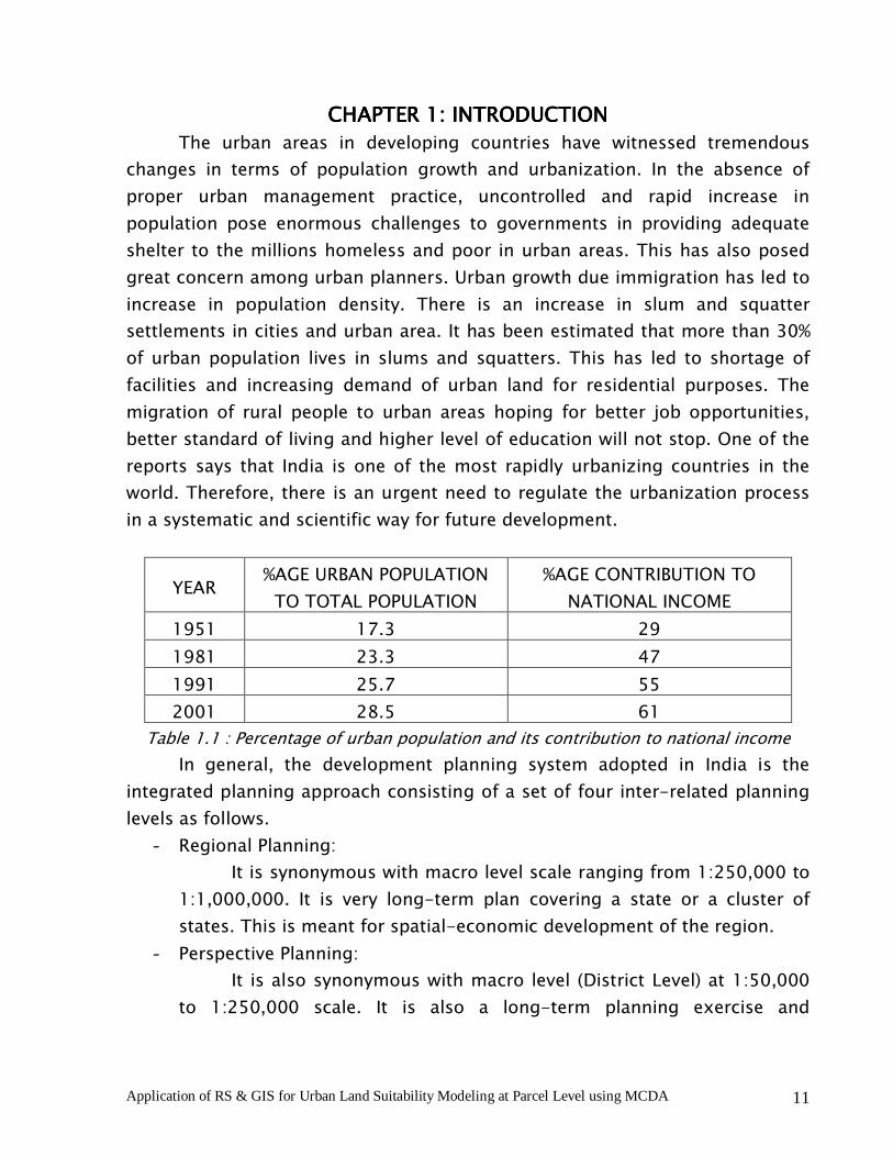
The urban areas in developing countries have witnessed tremendous
changes in terms of population growth and urbanization. In the absence of
proper urban management practice, uncontrolled and rapid increase in
population pose enormous challenges to governments in providing adequate
shelter to the millions homeless and poor in urban areas. This has also posed
great concern among urban planners. Urban growth due immigration has led to
increase in population density. There is an increase in slum and squatter
settlements in cities and urban area. It has been estimated that more than 30%
of urban population lives in slums and squatters. This has led to shortage of
facilities and increasing demand of urban land for residential purposes. The
migration of rural people to urban areas hoping for better job opportunities,
better standard of living and higher level of education will not stop. One of the
reports says that India is one of the most rapidly urbanizing countries in the
world. Therefore, there is an urgent need to regulate the urbanization process
in a systematic and scientific way for future development.
YEAR %AGE URBAN POPULATION
TO TOTAL POPULATION
%AGE CONTRIBUTION TO
NATIONAL INCOME
1951 17.3 29
1981 23.3 47
1991 25.7 55
2001 28.5 61
Table 1.1 : Percentage of urban population and its contribution to national income
In general, the development planning system adopted in India is the
integrated planning approach consisting of a set of four inter-related planning
levels as follows.
- Regional Planning:
It is synonymous with macro level scale ranging from 1:250,000 to
1:1,000,000. It is very long-term plan covering a state or a cluster of
states. This is meant for spatial-economic development of the region.
- Perspective Planning:
It is also synonymous with macro level (District Level) at 1:50,000
to 1:250,000 scale. It is also a long-term planning exercise and

Application of RS & GIS for Urban Land Suitability Modeling at Parcel Level using MCDA 12
addresses the policy issues relating to the spatial-economic development
of the district or cluster of districts.
- Development Planning:
It is synonymous with the meson-level (Block Level) at 1:25,000 to
1: 50,000 scale. It is conceived within the framework of sanctioned
perspective plan.
- Project Planning:
It is synonymous with micro-level (village level) at a scale from
1:5,000 to 1:500. It is detailed annual work layout for the executing
agency. It is prepared within the framework of Development Plan
The Above development planning exercises have to be viewed in the
context of specific problems associated with developing countries which
emanates primarily due to rapid population growth and limited resource
availability resulting in regional and intra-district imbalances at the socio-
economic development levels. These problems find further manifestation in the
form of low income levels, smaller land holdings, poor social services, inferior
infrastructure, poor literacy and hygiene, environmental degradation etc. Also
in context of spatial planning support in India, following problems are
encountered
- non-availability of country wide latest topographic and cadastral
database
- non-availability of technological know-how at working level
- lack of institutional back-up for implementing and monitoring the
development plans
- Security restriction problems related to the use of topographic database
or high resolution spatial data.
Urban planning is a complex phenomenon that requires enormous data
to support the decision. It is a process of identifying problems and finding
solutions using an information system.
Urbanization is a dynamic phenomenon, which keeps on changing with
time. Therefore, accurate and timely data is required for proper urban planning.
Urban planners use variety of data and methods to solve the problems of urban
areas. With the launch of artificial satellites and availability of remotely sensed
data, which gives synoptic view of the planning areas, the urban planners are
equipped with new tool. Today very high resolution data such as 1m PAN from

Application of RS & GIS for Urban Land Suitability Modeling at Parcel Level using MCDA 13
IKONOS, 0.6m PAN from QUICKBIRD and 2.5m PAN from CARTOSAT-1 satellites
are available at reasonable cost. This spatial data combined with other data can
provide better ability to understand the urban problems clearly and arrive at
suitable solutions. Spatial Expert Support System (SESS) can be used to analyze
complex relationships that have been difficult to handle by traditional methods.
It is a tool that can make integrated analysis possible and allow planners to
design models for development and to determine the various solutions
available to government to deal with rapid growth of cities and deterioration of
the environment. The urban planners need authenticated and accurate data and
sophisticated computer tools for making dynamic decisions. Remote sensing
and GIS are such tools or aids, which help the planners to accurately create and
manage data. GIS is used as analysis tool as a means of specifying logical and
mathematical relationships among map layers to get new derivative map layers.
Any new data can be added to existing GIS database easily. Thus remote
sensing data provides reliable, timely, accurate and periodic spatial data while
GIS provides various integrating tools for handling spatial and non-spatial data
to arrive at solution for decision making.
Successful implementation of Decision Support System (DSS) depends on
designing or choosing a right system that reflects the degree of problem
structure. Structured versus unstructured decision problems is the core of
concept of designing the DSS. The decision problems can be
- Structured or well defined either by decision-maker or on the basis of
appropriate theory,
- Unstructured or improperly or ill defined without any basis of
appropriate theory. Structured decisions can be programmed whereas
unstructured decisions can not be programmed. However, most real-life
problems lie in between two extremities called as semi-structured
decision problems. This is the area where DSS can play a major role.
Land or site suitability analysis for urban development falls within the
semi-structured decision problem category. Multi-Criteria Spatial Decision
Support System (MC-SDSS) and Spatial Expert Support System (SESS) both can
be utilized in the decision-making process. The key difference is that the
objective SDSS is to support decision making rather than to replace decision
maker while SESS focuses on providing a recommendation to the user based on
expert knowledge or replace a decision maker.

Application of RS & GIS for Urban Land Suitability Modeling at Parcel Level using MCDA 14
Figure 1.1: Unstructured and structured problems
• Aims and Objectives:Aims and Objectives:Aims and Objectives:Aims and Objectives:
The objective of the present study is to use Remote Sensing and GIS
techniques for Urban Land Suitability Modeling at parcel level using Multi-
Criteria Decision Analysis.
This study involves
- mapping of study area at parcel level using cadastral maps
- site suitability analysis using various parameters for urban
development
• Data Used:Data Used:Data Used:Data Used:
- Remote sensing satellite data:
Quick-Bird satellite data has been used with the following specifications as
given in the Table 1.2
Date of Acquisition 24th Feb 2004 Acquisition
Client KSRSAC, Bangalore
Date of launch 18th Oct’ 2001 Launch
Information Launch site SLC_2W,Vandenberg Airforce Base,
California, USA
Altitude 450 Km, Sun-synchronous
inclination Orbit
Revisit frequency 1 to 3.5 days depending on
latitude at 70 Cm resolution
Per-orbit
collection 128 GB ( 57 single area images )
DEGREE OF PROBLEM STRUCTURE
DECISION
COMPUTER
COMPUTER& DECISION

Application of RS & GIS for Urban Land Suitability Modeling at Parcel Level using MCDA 15
Nominal swath width 16.5 Km at nadir
Accessible ground
swath
544 Km centered on the satellite
ground track ( to ~ 30o off nadir)
Single area – 16.5 Km X 16.5 Km
Swath width &
area size
Areas of interest Strip - 16.5 Km X 165 Km
Circular error 23 m Metric
Accuracy Linear error 17 m
PAN 61 cm GSD at nadir Spatial
Resolution MSS 2.44 m GSD at nadir
PAN 445 – 900 nm
Blue : 450 – 520 nm
Green : 520 – 600 nm
Red : 630 – 690 nm
Spectral
Resolution MSS
NIR : 760 – 900 nm
Table 1.2: Specifications of Quick Bird satellite
- Cadastral maps:Cadastral maps:Cadastral maps:Cadastral maps:
The Cadastral maps or land records have been evolved on a varying scale
from 1:3500 to 1:8000 for the purpose of revenue collection by British Empire
in India. These maps have become obsolete due to irregular statutory surveys.
Therefore, the cadastral maps sometimes do not represent the true picture of
ground reality with respect to ownership and possession. The accuracy of
cadastral maps is less due to use of conventional chain and compass surveying
at that time. The conventional cadastral system is a multi-purpose system
catering to the needs of legal, fiscal, planning and other administrative
requirements. A cadastral map essentially comprises of land records of each
village, which were created by an aggregation of the graphical sketches of
individual land holdings and descriptive details of land parcels such as title and
extent. A village is the smallest administrative unit having well-defined
geographical boundary and separate land records.

Application of RS & GIS for Urban Land Suitability Modeling at Parcel Level using MCDA 16
- Topographical maps:Topographical maps:Topographical maps:Topographical maps:
Survey of India (SOI) topographic maps on scale of 1:50000 have been
used for identification of villages and guide map on 1:20000 for identifying
road network.
SOI MapSOI MapSOI MapSOI Map ScaleScaleScaleScale Year of SurveyYear of SurveyYear of SurveyYear of Survey Year of publicationYear of publicationYear of publicationYear of publication
57H9, 57H13 1:50000 1971-72 1973
Guide map 1:20000 1997-99 2002
Table 1.3: SOI maps
- Software used:Software used:Software used:Software used:
Erdas Imagine 8.5 version
Arc/Info 8.3
Arc Map
Arc View 3.2a
Microsoft Office 2000
• Scope and Limitations:Scope and Limitations:Scope and Limitations:Scope and Limitations:
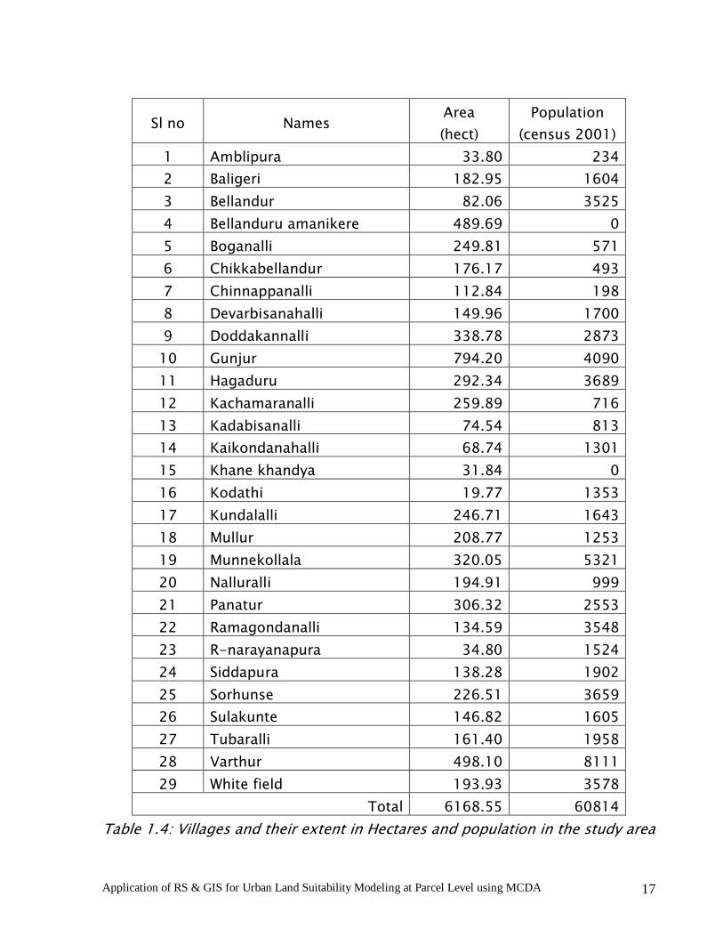
1. Bangalore urban district consists of totally 865 villages and practically it
is impossible to cover all villages for the project work due to limited
project time and constraints on finance and human resources.
2. Therefore, the following 29 villages are considered for study area as in
table 1.4
3. The detailed analysis is done for only one village i.e. Gunjur
Application of RS & GIS for Urban Land Suitability Modeling at Parcel Level using MCDA 17
Sl no Names Area
(hect)
Population
(census 2001)
1 Amblipura 33.80 234
2 Baligeri 182.95 1604
3 Bellandur 82.06 3525
4 Bellanduru amanikere 489.69 0
5 Boganalli 249.81 571
6 Chikkabellandur 176.17 493
7 Chinnappanalli 112.84 198
8 Devarbisanahalli 149.96 1700
9 Doddakannalli 338.78 2873
10 Gunjur 794.20 4090
11 Hagaduru 292.34 3689
12 Kachamaranalli 259.89 716
13 Kadabisanalli 74.54 813
14 Kaikondanahalli 68.74 1301
15 Khane khandya 31.84 0
16 Kodathi 19.77 1353
17 Kundalalli 246.71 1643
18 Mullur 208.77 1253
19 Munnekollala 320.05 5321
20 Nalluralli 194.91 999
21 Panatur 306.32 2553
22 Ramagondanalli 134.59 3548
23 R-narayanapura 34.80 1524
24 Siddapura 138.28 1902
25 Sorhunse 226.51 3659
26 Sulakunte 146.82 1605
27 Tubaralli 161.40 1958
28 Varthur 498.10 8111
29 White field 193.93 3578
Total 6168.55 60814
Table 1.4: Villages and their extent in Hectares and population in the study area

Application of RS & GIS for Urban Land Suitability Modeling at Parcel Level using MCDA 18
Chapter 2 : Cadastral MappingChapter 2 : Cadastral MappingChapter 2 : Cadastral MappingChapter 2 : Cadastral Mapping
• Introduction:Introduction:Introduction:Introduction:
The Cadastre is one of the country's basic registers. It shows individual
cadastral units of land-ownership and parcels and areas separated from them
that originally compiled for purposes of taxation. For many decades, traditional
cadastral systems have tended to enjoy a reputation for reliability, well defined
processes, and a well recognized guarantee of security of private land
ownership. Tremendous technological progress, social change, globalization,
and the increasing interconnection of business relations with their legal and
environmental consequences, however, have put a strain on the traditional
systems. They cannot adapt to all the new developments. An obvious indication
of this is the many reforms that cadastral systems are going through.
Cadastre is a methodically arranged public inventory of data concerning
properties within a certain country or district, based on a survey of their
boundaries. Such properties are systematically identified by means of some
separate designation. The outlines of the property and the parcel identifier
normally are shown on large-scale maps which, together with registers, may
show for each separate property the nature, size, value and legal rights
associated with the parcel. Land registration and cadastre usually complement
each other, they operate as interactive systems. Land registration puts in
principle the accent on the relation subject-right, whereas cadastre puts the
accent on the relation right-object. According to United Nations report
(ECOSOC E/1322 of 1949), Cadastral surveys, unlike scientific surveys of an
informative character which may be amended with changing conditions or
because they are not executed according to the standards now required for
accuracy, cannot be ignored, repudiated, altered or corrected, and the
boundaries created or re-established cannot be changed so long as they
control rights vested in the lands affected.
In developing countries cadastral surveying and cadastral mapping are
often criticized for being slow and expensive, and one of the major limitations
on economic development. Yet most authorities would agree that some form of
cadastral mapping in developing countries is essential for economic
development and environmental management.

Application of RS & GIS for Urban Land Suitability Modeling at Parcel Level using MCDA 19
• History Of Cadastral Maps:History Of Cadastral Maps:History Of Cadastral Maps:History Of Cadastral Maps:
The raw cadastral map (Figure 2.2) or land records (on the scale varying
between 1: 3500 & 1: 8000 scale) in India have evolved almost a century ago,
but they have remained practically unchanged till date. The statutory periodic
resurveys for creation of up-to-date land records were also not conducted in
the last 7 to 8 decades. Consequently, the cadastral maps are out of tune with
today's developmental imperatives and are unable to serve the contemporary
requirements.
The present cadastral system was evolved by the British for the purpose
of revenue collection and management. These cadastral maps were required to
be updated every 30 years. However, most of the states have not carried out
any survey and settlement operations at frequent intervals. Hence, the cadastral
maps are by and large out-dated and do not reflect the ground realities with
regard to ownership and possession. The accuracy of the original cadastral
surveys, which were carried out based on the technology and standards relevant
at that time, are wholly inadequate now due to rapid technological
advancements and achievements.
The conventional system in Karnataka as well as in India is a
multipurpose cadastral system catering to legal, fiscal and other administrative
requirements like planning and monitoring development programmes. This
essentially comprises of land records of each village, which are created by an
aggregation of the graphical sketches of individual landholdings and the
descriptive details of the land parcels such as title and extent. Village is the
smallest statutorily recognized administrative unit, having well-defined
geographical boundary and separate land records. A typical cadastral map
(1:7920 scale) representing a village in Karnataka is given in Figure 2.2. and the
legend of topographical features represented in these cadastral maps is given
in Figure 2.3. These records satisfied the minimum requirements such as
showing the reputed ownership of the landholder, the extent of land owned by
him, and in some case the landuse, land revenue etc. In some parts of the
country, the conventional land records comprised of additional details such as
irrigation facilities, agricultural/crop statistics, location-based remission of
taxation and livestock census. There are no common standard scales being
followed. The scale of cadastral maps varies from 1:3500 to 1:8000. Also,
these maps have not been updated over the years.

Application of RS & GIS for Urban Land Suitability Modeling at Parcel Level using MCDA 20
The digital cadastral map is the fundamental component of any cadastral
system. Its major advantage is that it displays the spatial relationships between
features depicted on it that contain two basic types of map information, Spatial
information, which describes the location and shape of geographic features and
their spatial relationships to other features and descriptive information about
the features.
The typical digital cadastral maps can speed up the processes of field
survey, the storage, retrieval and analysis of data, and the preparation and
production of cadastral maps and plans. This has two advantages - it reduces
the human mistakes that occur in writing down and subsequently transcribing
field survey observations, and it facilitates the transfer of data for subsequent
computation and adjustment. While new surveys may benefit from the
availability of computer systems, many maps already exist only on paper, for
example in written records or on paper maps. Old maps must be converted into
computer-readable form if the advantages of modern information technology
are to be realized. The conversion of these existing maps and graphic images
into digital form is usually done by “digitizing”. The technology for digitizing
maps is readily available, though the processes are often labour intensive and
remain expensive. The priority in many cadastral systems is to manage textual
records more efficiently rather than to produce digital cadastral maps. Text
data may include the property reference number, the name and address of the
proprietor, the title number and form of tenure, details of any mortgages,
subleases or assignments, any caveats, and possibly details of annual rents and
rental payments and their due dates. In addition there may be references to
survey plans, land-use zones, planning applications, etc.
• Advantages Of Cadastral Maps:Advantages Of Cadastral Maps:Advantages Of Cadastral Maps:Advantages Of Cadastral Maps:
The main advantages of computerization of cadastral maps are as
follows.
- Speed up the collection and processing of cadastral survey data;
- Make significant reductions in the cost and space required for storing and
retrieving land records;
- Prevent unnecessary duplication of records;
- Simplify the preparation of “back-up” copies of registers in case of
disaster;
- Accelerate the processing of data for the first registration of title;

Application of RS & GIS for Urban Land Suitability Modeling at Parcel Level using MCDA 21
- Reduce the time and cost involved in transferring property rights and in
processing mortgages;
- Facilitate the monitoring and analysis of land and property;
- Provide better estimates of the value of land for taxation or compulsory
acquisition;
- Improve efficiency and effectiveness in collecting land and property
taxes;
- Assist the compilation of information and reports that were impossible or
very cumbersome to produce using manual systems;
- Provide mechanisms for quality control;
- Integrate the records of land ownership, land use and land value with
socio-economic and environmental data in support of physical planning;
- Assist in the allocation and monitoring permits to build on land;
- Manage property assets and ensure their efficient use and maintenance;
- Document and monitor archaeological sites and other areas of scientific
or cultural interest;
- Record tree preservation orders and conservation areas;
- Support the management of utilities such as water, sewerage, gas,
electricity, street lights, and telephones;
The scale of cadastral maps is of great importance. Since the object of
the map is to provide a precise description and identification of the land, the
scale must be large enough for every separate plot of land which may be the
subject of separate possession (conveniently called a “survey plot” or “land
parcel”) to appear as a recognizable unit on the map. When map data are stored
in a computer, they may be drawn at almost any scale and this can give an
impression of greater accuracy than the quality of the survey data may warrant.
Large-scale plans are initially much more expensive to make per unit area than
small-scale maps, but it must always be remembered that, once the large-
scale survey has been completed; accurate maps on any smaller scale can be
derived from them. The converse is not however true for although larger-scale
maps can easily be constructed by using computers.

Application of RS & GIS for Urban Land Suitability Modeling at Parcel Level using MCDA 22
Figur
e 2.1: A typ
ical C
adas
tral M
ap (Gun
jur Villag
e, B
anga
lore
Urb
an S
outh
Tq.)

Application of RS & GIS for Urban Land Suitability Modeling at Parcel Level using MCDA 23
Figure 2.2: Legend for Cadastral Maps

Application of RS & GIS for Urban Land Suitability Modeling at Parcel Level using MCDA 24
• Role Role Role Role Of RS And GIS In Cadastral Mapping:Of RS And GIS In Cadastral Mapping:Of RS And GIS In Cadastral Mapping:Of RS And GIS In Cadastral Mapping:
By far, Aerial photography played an important role in cadastral mapping.
Aerial photos will be accurate and provide quicker results compared to manual
surveying. But, the preparation of base maps from aerial photos involves high-
cost and sophisticated photogrammetric equipments. On the other hand,
satellite remote sensing is the quickest and cheapest available method for
mapping. The availability of high-resolution satellite imagery of less than 1m
resolution provides the best accuracy that is needed for cadastral level mapping
at 1: 4000 or even larger, for the purpose of developmental activities. With the
launching of high-resolution satellites, the Remote Sensing technology has
opened a new era in cadastral updating. Quickbird, a satellite launched by US
based corporate Digital Globe Inc., is providing images of resolution of 61
centimeter, and as on today, it is the only satellite providing highest spatial
resolution in the civilian market. This will facilitate the geo-referencing of the
cadastral maps as well as mapping of any ground feature with measurements of
one meter by one meter. The landuse/landcover, hydro geomorphology, soil,
drainage and transport information can be extracted from the PAN sharpened
multi-spectral imageries of Quickbird. Hence, remote sensing facilitates the
updating of the cadastral maps after bringing into digital domain along with
information on natural resources. In the proposed project, it is intended to use
Quickbird satellite data.
The process of the digital cadastral maps can be undertaken using what
have become known as Geographic Information Systems or GIS. This technology
has dictated and influenced many changes in the development of land
administration and cadastral systems, with more specialized spatial
information. The GIS technology for data management, manipulation, analysis
and integration arguably has had the greatest impact on the spatial information
environment, although in the future the communication technologies are
rapidly becoming the focus of attention. These technologies are expected to be
the norm for viewing, locating and using land related information in the years
ahead. It is accepted that when cadastral information is part of integrated
information systems, it can improve the efficiency of the land transfer process
as well the overall land management process.

Application of RS & GIS for Urban Land Suitability Modeling at Parcel Level using MCDA 25
A GIS consists of a data base, graphic facilities and software for data
processing. Using a GIS, different data can be retrieved from the database, or
data can be taken from two or more data sets and overlaid on the graphic
screen or printed out on hard copy such as paper.
• Cadastral Issues and Limitations:Cadastral Issues and Limitations:Cadastral Issues and Limitations:Cadastral Issues and Limitations:
- National level policies for appropriate land recordsNational level policies for appropriate land recordsNational level policies for appropriate land recordsNational level policies for appropriate land records:
The unsystematic land survey and land records are the major issues for
proper management of land. The administrators, planners and decision makers
feel that one of the major factors for delay in execution of land related projects
is the lack of information. Availability of modern methods of surveying and
mapping required to be adopted for generating a uniform system of maps and
to be associated with the land records available in the country.
---- Coordinated efforts:Coordinated efforts:Coordinated efforts:Coordinated efforts:
There is need to identify and adopt appropriate technology for collecting
cadastral data. Computerization of land records and their updating in a
consistent format is also needed to make macro planning. Establishment of a
system to develop HRD strategy and institutional arrangement in support of
national LIS are required to be framed. In addition to this, there is need to
create standards at national level for cadastral surveys, equipment, methods,
data measurement, data structure, scale, accuracy, symbology and data
exchange format.
---- Cadastral maps on national datum :Cadastral maps on national datum :Cadastral maps on national datum :Cadastral maps on national datum :
Cadastral map data base to be integrated with national datum so that the
Individual land parcel and the rights of the land holders in the parcel get prime
focus in all developmental activities launched by the government.
The existing cadastral systems have the following limitations:
---- Mapping standards:Mapping standards:Mapping standards:Mapping standards:
In India the mapping standards are set by the Survey of India (SOI) and
ideally all the mapping tasks at local level – cadastral level have to follow these
standards. But the existing maps do not conform to the general mapping
standards practiced by SOI.
---- Dimensional accuracy: Dimensional accuracy: Dimensional accuracy: Dimensional accuracy:
Any standard mapping exercise takes care of the dimensional accuracy by
following appropriate co-ordinate systems and projection parameters. In the
present case, these features are not according to the prescribed standards that

Application of RS & GIS for Urban Land Suitability Modeling at Parcel Level using MCDA 26
have been followed at the national level by SOI. Hence, the dimensional
accuracy varies largely.
---- Geo Geo Geo Geo----referencing:referencing:referencing:referencing:
All the cadastral maps of the State have been created without any geo-
referencing in terms of latitude and longitude. This makes it extremely difficult
to position or reference cadastral parcels and villages in a spatial environment.
---- Mosaicing and edge match of adjacent maps: Mosaicing and edge match of adjacent maps: Mosaicing and edge match of adjacent maps: Mosaicing and edge match of adjacent maps:
Due to the inherent reasons resulting due to non-compliance with the
survey of India standards, the adjacent maps of even a small region do not form
a seamless mosaic. The cadastral maps highlight that after clipping of
concerned village maps, there are overlaps and gaps along the borders of the
villages as the number of villages increased for mosaicking and there are no
continuation of permanent features like hills and streams in its adjacent
villages.
---- Topographic features on maps: Topographic features on maps: Topographic features on maps: Topographic features on maps:
The information captured in the cadastral map is very limited – more
emphasis has been on mapping only the land parcel boundaries. Survey number
information is the only attribute information available for a land parcel.
---- Bench Marks:Bench Marks:Bench Marks:Bench Marks:
Permanent immovable benchmarks placed by SOI are to be used as
standard reference marks for surveying. The cadastral maps have been created
using benchmarks that have no protection and are prone to human
interference. This has resulted in inaccuracy while resurveying.
- Updating new partitions:Updating new partitions:Updating new partitions:Updating new partitions:
The current practice of updating new partitions in land parcels is not
Oriented towards updating the original village map, instead an addendum
called Tippany is created – which holds a rough sketch of the area with
dimensions written across its boundaries along with the schedule of the
property.
Though there is a considerable effort involved in collecting the new
partition information, the very purpose of updating land information is not
completely realized. This is primarily due to the incompatibility between the
geo-referencing environments present in the map and the data recorded during
the partition survey.

Application of RS & GIS for Urban Land Suitability Modeling at Parcel Level using MCDA 27
Chapter 3: Basic Concepts of Remote Sensing and GISChapter 3: Basic Concepts of Remote Sensing and GISChapter 3: Basic Concepts of Remote Sensing and GISChapter 3: Basic Concepts of Remote Sensing and GIS
• Remote Sensing:Remote Sensing:Remote Sensing:Remote Sensing:
Remote sensing, in the simplest words, means acquiring information
about an object without touching the object itself. Conveniently, however,
remote sensing has become to imply that the sensor and target are located
remotely apart and the electromagnetic radiation serves as a link between
sensor and the object, the sun being the major source of energy illuminating
the earth. The pat of this energy is reflected, absorbed and transmitted by the
surface. A sensor records the reflected energy.
Remote sensing can then be defined as “The technique about an object
by a recording device or sensor that is not in physical contact with the object by
measuring portion of reflected or emitted electromagnetic radiation from the
earth’s surface.”
Figure 3.1: Energy interactions in the atmosphere
• Fundamental Principle Of Remote Sensing:Fundamental Principle Of Remote Sensing:Fundamental Principle Of Remote Sensing:Fundamental Principle Of Remote Sensing:
The basic principle involved is that the different objects based on their
structural, chemical and physical properties return (reflect or emit) different
amount of energy in different wavelength ranges (commonly referred to as
BANDS) of the electromagnetic spectrum incident upon it. Most remote sensing
programmes utilize the sun’s energy, which is a predominant source of energy.
These radiations travel through the atmosphere and are selectively scattered

Application of RS & GIS for Urban Land Suitability Modeling at Parcel Level using MCDA 28
and/or absorbed depending upon the composition of the atmosphere and the
wavelength involved. These radiations upon reaching the earth’s surface
interact with the target objects (earth surface features). Everything in nature has
its own unique pattern of reflected, emitted and absorbed radiation. A sensor is
used to record reflected or emitted energy from the surface. This recorded
energy is then transmitted to the users and it is processed to form an image,
which is then analyzed to extract information about the target. Finally the
information extracted is applied to assist in decision making for solving a
particular problem. Thus we can summarize the remote sensing process in the
following seven steps, which are depicted in Figure 3.2.
Figure 3.2: Stages in Remote Sensing process
• Stages in Remote Sensing Process:Stages in Remote Sensing Process:Stages in Remote Sensing Process:Stages in Remote Sensing Process:
---- Energy source Energy source Energy source Energy source: The first requirement for remote sensing is to have an
energy source, which illuminates the target of interest
---- Energy interactions with the atmosphere Energy interactions with the atmosphere Energy interactions with the atmosphere Energy interactions with the atmosphere: The energy on its way from
source to target and then, from target to the sensor comes in contact and
interacts with the atmosphere.
---- Interactions of energy with earth’s surface fe Interactions of energy with earth’s surface fe Interactions of energy with earth’s surface fe Interactions of energy with earth’s surface featuresaturesaturesatures: Different earth’s
surface features react differently to the incident energy. Portions of incident
energy are reflected, transmitted or absorbed by the surface.
---- Recording of energy by the sensor: Recording of energy by the sensor: Recording of energy by the sensor: Recording of energy by the sensor: The energy after interacting with
earth’s surface reaches the sensor (which is remote – not in touch with the

Application of RS & GIS for Urban Land Suitability Modeling at Parcel Level using MCDA 29
earth surface features) where it is recorded in a form, which can be
transmitted to and used by the users.
---- Data transmission and processing Data transmission and processing Data transmission and processing Data transmission and processing: The energy recorded by the sensor
is transmitted to a receiving and a processing station where the data are
processed into an image.
---- Image processing and analysis: Image processing and analysis: Image processing and analysis: Image processing and analysis: The processed image is interpreted to
extract the information about the earth’s surface features.
---- Application: Application: Application: Application: The extracted information is then utilized to make
decisions for solving particular problems.
Thus remote sensing is a multidisciplinary science, which includes a
combination of various disciplines such as optics, photography, computer,
electronics and telecommunication, satellite launching etc.
• Passive And Active Remote Sensing:Passive And Active Remote Sensing:Passive And Active Remote Sensing:Passive And Active Remote Sensing:
The sun provides a very convenient source of energy for remote sensing.
The sun’s energy is either reflected, as it is for visible wavelength or absorbed
and then re-emitted (for thermal infrared wavelength).
Figure 3.3: Passive sensors
Remote sensing systems, which measure this naturally energy, are called
as passive sensors. This can only take place when the sun is illuminating the
earth. There is no reflected energy available from the sun at night. Energy that
is naturally emitted can be detected day or night provided that the amount of
energy is large enough to be recorded.

Application of RS & GIS for Urban Land Suitability Modeling at Parcel Level using MCDA 30
Figure 3.4: Active Sensors
Remote sensing systems, which provide their own source of energy for
illumination, are known as active sensors. These sensors have the advantage of
obtaining data at any time of day or season.
Solar energy and radiant heat are examples of passive energy sources,
synthetic aperture Radar (SAR) is an example of active sensor.
In order to collect and record energy reflected or emitted from a target or
source, we require a sensing device (commonly called as sensor) residing on a
stable platform.
• Platforms:Platforms:Platforms:Platforms:
Platform is a stage to mount the camera or sensor to collect information
remotely about an object or surface. Platforms for remote sensors may be
situated on the ground, on an aircraft or balloon or on a spacecraft or satellite
outside of the earth’s atmosphere (Figure 3.5)
Ground-based sensors are often used to record detailed information
about the surface. In these systems sensors may be placed on a ladder, tall
building, crane etc.
Aerial platforms are aircrafts, which are primarily used to acquire aerial
photographs. Airplanes are used to collect very detailed images over any
portion of earth at any time. Balloons were also used to acquire aerial
photographs. Airplanes are also used to test the sensors before they can be put
onboard satellites.

Application of RS & GIS for Urban Land Suitability Modeling at Parcel Level using MCDA 31
The platforms in space (satellites) are not affected by earth’s atmosphere.
Satellites are objects; the moon is a natural satellite, whereas manmade
satellites include those platforms launched for remote sensing, communication
and telemetry (location and navigation) purposes. These satellites freely move
in their orbits around the earth and any part of the earth can be covered at
specified time intervals. It is these satellites that we get enormous amount of
remotely sensed data about earth’s surface.
Figure 3.5: Ground, Air and Space Borne Remote Sensing
• Satellite Orbits:Satellite Orbits:Satellite Orbits:Satellite Orbits:
The path followed by a satellite is referred to as its orbit. Satellites can be
categorized as Geostationary or near polar based on their orbits and altitude
(height above earth’s surface) as shown in Figure 3.6.
Figure 3.6: Satellite orbits

Application of RS & GIS for Urban Land Suitability Modeling at Parcel Level using MCDA 32
---- Geostationary Satellites: Geostationary Satellites: Geostationary Satellites: Geostationary Satellites:
The geostationary satellites are located at very high altitudes of
approximately 36,000 KM above the earth. They revolve at speed which
matches the rotation of the earth (24 hours) so they seem stationary, relative to
the earth’s surface and hence view one-third of globe. These satellites are used
for weather monitoring and communication.
---- Polar or Sun Polar or Sun Polar or Sun Polar or Sun----Synchronous Satellites:Synchronous Satellites:Synchronous Satellites:Synchronous Satellites:
Remote sensing satellites are designed to follow an inclined north-south
orbit. A satellites in this orbit has an inclination that carries the satellite track
westward at a rate such that it covers each area of the world at constant time of
the day called as local sun time as the satellite moves from north to south. This
ensures similar illumination conditions when acquiring images over a particular
area over a series of days.
These satellites travel from north to south o the sunlit side of the earth.
This is the descending pass of the satellite, while in the ascending pass the
satellite travels from south to north and it is the shadowed side of the earth.
• ResolutResolutResolutResolution of Satellite Images: ion of Satellite Images: ion of Satellite Images: ion of Satellite Images:
In general resolution is defined as the ability of an entire remote-sensing
system, including lens antennae, display, exposure, processing, and other
factors, to render a sharply defined image. Resolution of a remote-sensing is of
different types.
- Spectral ResolutionSpectral ResolutionSpectral ResolutionSpectral Resolution: of a remote sensing instrument (sensor) is
determined by the band-widths of the Electro-magnetic radiation of the
channels used. High spectral resolution, thus, is achieved by narrow
bandwidths width, collectively, are likely to provide a more accurate spectral
signature for discrete objects than broad bandwidth.
- Radiometric Resolution:Radiometric Resolution:Radiometric Resolution:Radiometric Resolution: is determined by the number of discrete levels
into which signals may be divided.
---- Spatial Resolution: Spatial Resolution: Spatial Resolution: Spatial Resolution: in terms of the geometric properties of the imaging
system, is usually described as the instantaneous field of view (IFOV). The IFOV
is defined as the maximum angle of view in which a sensor can effectively
detect electro-magnetic energy. Table 3.1 shows the recommended spatial
resolutions for various planning levels and their applications.

Application of RS & GIS for Urban Land Suitability Modeling at Parcel Level using MCDA 33
----Temporal ResolutionTemporal ResolutionTemporal ResolutionTemporal Resolution: is related to the repetitive coverage of the ground
by the remote-sensing system. The temporal resolution of Landsat 4/5 is
sixteen days.
Low ResolutionLow ResolutionLow ResolutionLow Resolution Medium Medium Medium Medium ResolutionResolutionResolutionResolution High ResolutionHigh ResolutionHigh ResolutionHigh Resolution
80 – 360 m 20-40 m 1-5 m
Level of PlanningLevel of PlanningLevel of PlanningLevel of Planning Macro Level (Regional
& Perspective)
Meso Level ( District/
Development)
Micro Level ( Project,
Micro-watershed, Village)
Scale MappingScale MappingScale MappingScale Mapping 1: 50000 to
1:1000000
1:25000 to 1: 50000 1:1000 to 1:5000
Application AreaApplication AreaApplication AreaApplication Area Demonstrated Applications Prospects
Crop acreage and Crop acreage and Crop acreage and Crop acreage and
Production ForecastProduction ForecastProduction ForecastProduction Forecast
Mono-crop areas - large
extents
Multi-crop areas -
medium extents
Mix-crop areas
-Cropping System Studies
-Parcel size for crops
grown
- input to precision
farming
Landuse PlanningLanduse PlanningLanduse PlanningLanduse Planning -Land use mapping at
Level-1 classification
-Wasteland mapping at
level-1
-Wetland mapping at
level-1
-Mapping at Level
2/3 classification
(Taluk/mandal level)
-Land use change
analysis
-Wasteland mapping
at level-2/3
-Wetland mapping
at level-2/3
- Cadastre/ field level
mapping - classification
level – 3 & 4
(Village/mandal)
- Inputs for tourism
development
Rural Development Rural Development Rural Development Rural Development
PlanningPlanningPlanningPlanning
-Regional maps
-Settlement network
-Land and water
resources
-development maps
-Cadastral level landuse
maps
-Land parcel maps
-Micro level watershed/
village planning
Urban PlanningUrban PlanningUrban PlanningUrban Planning -Urban Sprawl analysis
-Urban land use at
level1
-Transportation network
(Highways, Railways
etc.)
-Urban landuse
mapping (level-1)
-Urban suitability
analysis
-Mapping of major
transport network
Updating of city
guide maps
-Urban landuse mapping
(level 1 & 2)
-Slum typology
-Mapping of street level
-Urban road network
-Mapping of property
parcels Inputs for
infrastructure development

Application of RS & GIS for Urban Land Suitability Modeling at Parcel Level using MCDA 34
SoilsSoilsSoilsSoils -Soil family Association
mapping
-Land degradation
(Water logged, salt
affected, erosion prone)
-Soil series
association
-Land degradation
at level 2
-Soil series
-Land degradation at
micro level
Water ResourcesWater ResourcesWater ResourcesWater Resources -Watershed
characterization &
prioritization
-Glacier Inventory
-Groundwater
prospects
-Watershed
Prioritization
-Snow melt run-off
estimation
-Micro watershed planning
-Monitoring of
development schemes
-Drinking water site
selection
ForestForestForestForest -Forest type & density
Mapping
-Forest type &
density Mapping
-Detection of
degraded forest
areas
-Forest fire
monitoring
-Forest Species
identification
-Inputs for working plan
generation
-Habitat mapping
Biomass Estimation
Geology & MineralsGeology & MineralsGeology & MineralsGeology & Minerals Regional Geological
maps
Detailed geological
mapping
Oil, Gas and Mineral
Exploration
InfrastructureInfrastructureInfrastructureInfrastructure
PlanningPlanningPlanningPlanning
-Regional level corridor
planning
-Broad Site
Suitability analysis
-Mapping of major
road network
-Specific Project Site
Analysis
-Dams ,Highways ,Canal
Industries, Power Plants
DisasterDisasterDisasterDisaster -Flood Prone Area Maps
-Cyclone Monitoring
-Drought Monitoring &
Forecast
-Earthquake prone
areas
-Landslide prone area
mapping
-Slope stability mapping
-Post Disaster
Damage assessment
-Property Insurance
for Natural Disasters
-Post Disaster Relief
Management Support
-Tracing of approach
routes
-Waste disposal and solid
waste management
Meteorology & Meteorology & Meteorology & Meteorology &
OceanographyOceanographyOceanographyOceanography
-Monsoon Forecast
-Sea-surface temp
-Wind vectors
-Waves spectra
-Sea surface topography
- -
Table Table Table Table –––– 3.1: Satelli 3.1: Satelli 3.1: Satelli 3.1: Satellite Imagery for Different Levels of Development Planningte Imagery for Different Levels of Development Planningte Imagery for Different Levels of Development Planningte Imagery for Different Levels of Development Planning

Application of RS & GIS for Urban Land Suitability Modeling at Parcel Level using MCDA 35
Resolution(m)/Swath Width(km)Resolution(m)/Swath Width(km)Resolution(m)/Swath Width(km)Resolution(m)/Swath Width(km) Operational Operational Operational Operational
Systems Systems Systems Systems
SatelliteSatelliteSatelliteSatellite
Data Data Data Data
ProviderProviderProviderProvider PrimePrimePrimePrime LaunchLaunchLaunchLaunch
PANPANPANPAN MSSMSSMSSMSS RadarRadarRadarRadar
Repeat Repeat Repeat Repeat
Cycle Cycle Cycle Cycle
(days)(days)(days)(days)
LandsatLandsatLandsatLandsat----5555
ERSERSERSERS----2222
Radarsat1Radarsat1Radarsat1Radarsat1
IRSIRSIRSIRS----1C1C1C1C
Orbview2Orbview2Orbview2Orbview2
IRSIRSIRSIRS----1D1D1D1D
SpotSpotSpotSpot----4444
LLLLandsatandsatandsatandsat----7777
IRSIRSIRSIRS----P4P4P4P4
IkonosIkonosIkonosIkonos
Quick BirdQuick BirdQuick BirdQuick Bird
Cartosat1Cartosat1Cartosat1Cartosat1
EDC DAAC
Eurimage
Radarsat
Eosat,
NRSA
Orbimage
Eosat,
NRSA
Spot Image
EDC DAAC
NRSA
Space
Imaging
NRSA
NRSA
Orbital Sci.
Dornier
Spar
Aerospace
ISRO
Orbital Sci.
ISRO
Matra
Macroni
Orbital Sci.
ISRO
Eosat
Digital
Globe
ISRO
Mar-84
Apr-95
Nov-95
Dec-95
Aug-97
Sep-97
Mar-98
Apr-99
May-99
Sep-99
Oct-01
May-05
-
-
-
5.8/70
10/117
-
-
1/11x11
0.6/
16.5x16.5
2.5/
21.5x21.5
30-80 /185
36.25 /131
-
23.5-70.5
/142
1000/ 2800
23.5-70.5
/142
20/117
4000/1150
15/185
360/1420
4/11x11
2.4/
16.5x16.5
-
-
26/102
7.6-100
/
50-500
-
-
-
-
-
-
-
-
16
35
24
24
16
24
26
-
26
16
2
3
1to3.5
5
Table Table Table Table –––– 3.2: Oper 3.2: Oper 3.2: Oper 3.2: Operational Satellitesational Satellitesational Satellitesational Satellites

Application of RS & GIS for Urban Land Suitability Modeling at Parcel Level using MCDA 36
• Geographic Information System:Geographic Information System:Geographic Information System:Geographic Information System:
A geographic information system (GIS) is a computer based tool for
mapping and analyzing geographic phenomenon that exists and events that
occur on earth. GIS technology integrates common database operations such as
query and statistical analysis with the unique visualization and geographic
analysis benefits offered by maps. These abilities distinguish GIS from other
information systems and make it valuable to a wide range of public and private
enterprises for explaining events, predicting outcomes, and planning strategies.
Map making and geographic analysis are not new, but a GIS performs these
tasks faster and with more sophistication than do traditional manual methods.
In general, a GIS provides facilities for data capture, data management,
data manipulation and analysis and the presentation of results in both graphic
and report form, with a particular emphasis upon preserving and utilizing
inherent characteristics of spatial data.
The ability to incorporate spatial data, manage it, analyze it and answer
spatial questions is the distinctive characteristic of GIS.
A geographic information system, commonly referred to as GIS, is an
integrated set of hardware and software tools used for the manipulation and
management of digital spatial (geographic) and related attribute data.
• GIS Subsystems:GIS Subsystems:GIS Subsystems:GIS Subsystems:
A GIS has four main functional subsystems. These are
- data input subsystem
- data storage and retrieval subsystem
- data manipulation and analysis subsystem
- data output and display subsystem
- Data input:Data input:Data input:Data input:
A data input subsystem allows the user to capture, collect and transform
spatial and thematic data into digital form. The data inputs are usually derived
from a combination of hard copy maps, aerial photographs, remotely sensed
images, reports, survey documents etc as shown in figure 3.7.
- Data storage and retrieval:Data storage and retrieval:Data storage and retrieval:Data storage and retrieval:
The data storage and retrieval subsystem organizes the data, spatial and
attribute in the form which permits it to be quickly retrieved by the user for
analysis and permits rapid and accurate updates to be made to the database.
This component usually involves use of a database management system (DBMS)

Application of RS & GIS for Urban Land Suitability Modeling at Parcel Level using MCDA 37
for maintaining attribute data. Spatial data is usually encoded and maintained
in proprietary format.
Figure 3.7: Various data input devices/methods
---- Data manipulation and analysis: Data manipulation and analysis: Data manipulation and analysis: Data manipulation and analysis:
The data manipulation and analysis subsystem allows the user to define
and execute spatial and attribute procedures to generate derived information.
The subsystem is commonly thought if as the heart of a GIS, and usually
distinguishes it from other database information systems and computer aided
drafting (CAD) systems.
---- Data output: Data output: Data output: Data output:
The data output subsystem allows the user to generate graphic displays
normally maps and tabular reports representing derived information products.
• Components of GIS:Components of GIS:Components of GIS:Components of GIS:
An operational GIS also has a series of components that combine to make
the system work. A working GIS integrates five key components, namely
Hardware, Software, Data, People and Methods.
Figure 3.8: Components of GIS

Application of RS & GIS for Urban Land Suitability Modeling at Parcel Level using MCDA 38
- Hardware:Hardware:Hardware:Hardware:
Hardware is the computer system on which a GIS operates. Today, GIS
software runs on a wide range of hardware types, from centralized computer
servers to desktop computers used in stand-alone or networked configurations.
---- Software: Software: Software: Software:
GIS software provides the functions and tools needed to store, analyze,
and display geographic information.
---- Data: Data: Data: Data:
The most important component of a GIS is the data. Geographic data and
related tabular data can be collected in-house, compiled to custom
specifications and requirements, or occasionally purchased from a commercial
data provider. A GIS can integrate spatial data with other existing data
resources, often stored in a corporate DBMS. The integration of spatial data
(often proprietary to the GIS software) and tabular data stored in a DBMS is a
key functionality afforded by GIS.
---- People: People: People: People:
GIS technology is of limited value without the people who manage the
system and develop plans for applying it to real world problems. GIS users
range from technical specialists (who design and maintain the system) to those,
who use it in their everyday work. The identification of GIS specialists versus
end users is often critical to the proper implementation of GIS technology.
---- Methods: Methods: Methods: Methods:
A successful GIS operates according to a well-designed implementation
plan and business rules, which are the models and operating practices unique
to each organization.
• GIS Data Models:GIS Data Models:GIS Data Models:GIS Data Models:
GIS store information about the world as a collection of thematic layers
which can be linked together by geography. This simple but extremely powerful
and versatile concept has proven invaluable for solving many real-world
problems from tracking delivery vehicles, to recording details of planning
applications, to modeling global atmospheric circulation. The thematic layer
approach allows us to organize the complexity of the real world into a simple
representation to help facilitate our understanding of natural relationships.

Application of RS & GIS for Urban Land Suitability Modeling at Parcel Level using MCDA 39
Figure 3.9: GIS Thematic layers representing real world features
• GIS Data Types:GIS Data Types:GIS Data Types:GIS Data Types:
The basic data types in a GIS reflect traditional data found on a map.
Accordingly, GIS technology utilizes two basic types of data. These are:
- Spatial dataSpatial dataSpatial dataSpatial data – This describes the absolute and relative location of
Geographic features.
- Attribute dataAttribute dataAttribute dataAttribute data – which describes the characteristics of the spatial
features. These characteristics can be quantitative and/or qualitative in nature.
Attribute data is often referred to as tabular data.
The coordinate location of a forestry stand would be spatial data, while
the characteristics of the forestry stand, e.g. cover group, dominant species,
crown closure, height etc. would be attribute data.
• Spatial data models:Spatial data models:Spatial data models:Spatial data models:
Traditionally spatial data has been stored and presented in the form of a
map. Three basic types of spatial data models have evolved for storing
geographic data digitally. These are referred to as Vector, Raster and Image.
The following Figure 3.11 reflects the two primary spatial data encoding
techniques. These are vector and raster. Image data utilizes techniques very
similar to raster data, however typically lacks the internal formats required for
analysis and modeling of the data. Images reflect pictures or photographs of
the landscape.

Application of RS & GIS for Urban Land Suitability Modeling at Parcel Level using MCDA 40
Figure 3.10: Representation of the real world and showing differences in how a
vector and a raster GIS will represent this real world.
---- Vector Data Vector Data Vector Data Vector Data FormatFormatFormatFormat::::
All spatial data models are approaches for storing the spatial location of
geographic features in a database. Vector storage implies the use of vectors
(directional lines) to represent a geographic feature. Vector data is
characterized by the use of sequential points or vertices to define a linear
segment. Each vertex consists of an X coordinate and a Y coordinates.
Figure 3.11: Vector data format

Application of RS & GIS for Urban Land Suitability Modeling at Parcel Level using MCDA 41
Vector lines are often referred to as arcs and consist of a string of
vertices terminated by a node. A node is defined as a vertex that starts or ends
an arc segment. One coordinate pair, a vertex, defines point features. Polygonal
features are defined by a set of closed coordinate pairs. In vector
representation, the storage of the vertices for each feature is important, as well
as the connectivity between features, e.g. the sharing of common vertices
where features connect.
The vector data model does not handle continuous data, e.g. elevation,
very well while the raster data model is more ideally suited for this type of
analysis. Accordingly, the raster structure does not handle linear data analysis,
e.g. shortest path, very well while vector systems do. There are certain
advantages and disadvantages to each data model.
---- Ras Ras Ras Raster Data ter Data ter Data ter Data Format:Format:Format:Format:
Raster data models incorporate the use of a grid-cell data structure
where the geographic area is divided into cells identified by row and column.
This data structure is commonly called raster. While the term raster implies a
regularly spaced grid other tessellated data structures do exist in grid based
GIS systems. In particular, the quad tree data structure has found some
acceptance as an alternative raster data model.
Figure 3.12: Raster data format
Most raster based GIS software requires that the raster cell contain only a
single discrete value. Accordingly, a data layer, e.g. forest inventory stands,
may be broken down into a series of raster maps, each representing an

Application of RS & GIS for Urban Land Suitability Modeling at Parcel Level using MCDA 42
attribute type, e.g. a species map, a height map, a density map, etc. These are
often referred to as one attribute maps. This is in contrast to most conventional
vector data models that maintain data as multiple attribute maps, e.g. forest
inventory polygons linked to a database table containing all attributes as
columns. This basic distinction of raster data storage provides the foundation
for quantitative analysis techniques. This is often referred to as raster or map
algebra. The use of raster data structures allow for sophisticated mathematical
modeling processes while vector based systems are often constrained by the
capabilities and language of a relational DBMS.
• Spatial DatSpatial DatSpatial DatSpatial Data Relationships:a Relationships:a Relationships:a Relationships:
The nature of spatial data relationships is important to understand within
the context of GIS. The accepted theoretical solution is to topologically
structure spatial data.
Most GIS software segregate spatial and attribute data into separate data
management systems. Most frequently, the topological or raster structure is
used to store the spatial data, while the relational database structure is used to
store the attribute data. Data from both structures are linked together for use
through unique identification numbers, e.g. feature labels and DBMS primary
keys. An integral number assigned by the GIS software usually maintains this
coupling of spatial features with an attribute record for a given geographic
feature. Most often the GIS software is properly generated. This attribute’s
record once a clean topological structure is properly generated. This attribute
record normally contains the internal number for the feature, the user’s label
identifier, the area of the feature, and the perimeter of the feature. Linear
features have the length of the feature defined instead of the area.
• Topology:Topology:Topology:Topology:
Topology is a mathematical approach that allows us to structure data
based on the principles of feature adjacency and feature connectivity. It is in
fact the mathematical method used to define spatial relationships. Without a
topologic data structure, in a vector based GIS most data manipulation and
analysis functions would not be practical or feasible.

Application of RS & GIS for Urban Land Suitability Modeling at Parcel Level using MCDA 43
Chapter 4: MultiChapter 4: MultiChapter 4: MultiChapter 4: Multi----Criteria Decision Analysis (MCriteria Decision Analysis (MCriteria Decision Analysis (MCriteria Decision Analysis (MCDA):CDA):CDA):CDA):
• IntroductionIntroductionIntroductionIntroduction:
MCDA problems involve a set of alternatives that are evaluated on the
basis of conflicting and incommensurate criteria. Criterion can be an attribute
or objective. Accordingly MCDA can be classified into to categories, namely
Multi-Attribute Decision Analysis (MADA) and Multi-Objective Decision Analysis
(MODA). Both MADA and MODA problems are further classified into single
decision maker problems and group decision problems. These categories are
subdivided into deterministic, probabilistic and fuzzy decisions.
- Deterministic decision problems assume that the required data and
information are known with certainty and there is a deterministic relationship
between every decision and the corresponding decision sequence.
- Probabilistic analysis deals with a decision situation under uncertainty
with respect to available data and decision making sequence but treats
uncertainty as randomness.
- Fuzzy decision analysis also deals with a decision situation under
uncertainty with respect to available data and decision making sequence but
considers inherent imprecision of information involved in decision making.
COMPARISON OF MODA AND MADA
MODA MADA
Criteria defined by Objectives Attributes
Objectives defined Explicitly Implicitly
Attributes defined by Implicitly Explicitly
Constraints defined Explicitly Implicitly
Alternatives defined Implicitly Explicitly
No. of alternatives Large Small
Decision maker’s control Significant Limited
Relevant to Design/search Evaluation/choice
Decision modeling
paradigm Process oriented Outcome oriented
Data structure Vector based GIS Raster based GIS
Table 4.1: Comparison of MODA and MADA

Application of RS & GIS for Urban Land Suitability Modeling at Parcel Level using MCDA 44
• Elements of MultiElements of MultiElements of MultiElements of Multi----Criteria Decision Analysis (MCDA):Criteria Decision Analysis (MCDA):Criteria Decision Analysis (MCDA):Criteria Decision Analysis (MCDA):
MCDA problems involve six components:
- A goal or set goals the decision maker attempts to achieve
- The decision maker or group of decision makers involved in the
decision making process along with their preferences with respect to evaluation
criteria
- A set of evaluation criteria (objective and/or attributes) on the basis of
which the decision makers evaluate alternative courses of action
- The set of decision alternatives that is decision or action variables
- The set of uncontrollable variables
- The set of outcome or consequences associated with each pair.
The relationships between the elements of MCDA are shown in Figure-
4.1. The central element of this structure is a decision matrix consisting of a set
of columns and rows. The matrix represents the decision outcomes for a set of
alternatives and a set of evaluation criteria.
The structure of columns consists of levels representing the decision
makers, their preferences and evaluation criteria. These elements are organized
in a hierarchical structure. The rows of the decision matrix represent decision
alternatives. The decision outcomes depend on the set of evaluating
alternatives.
A criterion is a standard judgment or rule on the basis of which the
alternatives decisions are ranked according to their desirability. Criterion is a
generic term including the concept of attribute and objectives. Attribute
represents the properties of elements of a real world geographical system.
More specifically, an attribute is a measurable quantity or quality of
geographical entity or a relationship between geographical entities. An attribute
is used to measure performance in relation to an objective. An objective is a
statement about the desired state of the system under consideration. It
indicates the directions of improvement of one or more attributes. Objectives
are functionally related to or derived from a set of attributes
The state of nature or environment refers to the uncontrollable
environmental factors such as weather condition, physical condition, economy
etc. Each state is assumed to be independent of other states and immune to
manipulation by the decision makers. As such, the states of nature reflect the
degree of uncertainty about decision outcomes. Ultimately, the decision

Application of RS & GIS for Urban Land Suitability Modeling at Parcel Level using MCDA 45
problems require that the set of outcomes to be ordered so that the best
alternatives can be identified.
Figure 4.1: Relationship among the elements of MCDA
• Framework of Spatial MultiFramework of Spatial MultiFramework of Spatial MultiFramework of Spatial Multi----critercritercritercriteria Decision Analysis:ia Decision Analysis:ia Decision Analysis:ia Decision Analysis:
Framework organized in terms of the sequence of activities involved in
spatial multi-criteria analysis is shown in figure. It integrates the different
phases of decision-making and major elements of MCDA.
---- Problem definition:Problem definition:Problem definition:Problem definition:
Any decision making process begins with the recognition and definition
problem. It is a gap between the desired and existing states as viewed by a
decision maker. It overlaps the intelligence phase of decision making. The GIS
capabilities for data storage, management, manipulation and analysis offer
major support in the problem definition stage.
---- Evaluation criteria:Evaluation criteria:Evaluation criteria:Evaluation criteria:
Once decision problem is identified or defined, the spatial multi-criteria
analysis focuses on the set of evaluation criteria (i.e. Objectives and attributes).
A measurement scale must be established for each attribute. The degree to
which objectives are met, as measured by the attributes is the basis for
comparing alternatives. The evaluation criteria are associated with geographical
entities and therefore, relationships between entities, can be represented in the
Attribute1 Attribute2 Attribute3 ---- Attributen
Alternative1 Outcome11 Outcome12 Outcome13 ---- Outcome1n
Alternative2 Outcome21 Outcome22 Outcome23 ---- Outcome2n
Alternative3 Outcome31 Outcome32 Outcome33 ---- Outcome3n
------ ------ ------ ------ ---- ------
Alternativen Outcomen1 Outcomen2 Outcomen3 ---- Outcomenn
ST
AT
E O
F
EN
VIR
ON
MEN
T
Preferences Weight1 Weight2 Weight3 ---- Weightn
GOA
DECISION MAKER 1 DECISION MAKER 2
OBJECTIVE 1 OBJECTIVE 2 OBJECTIVE 3
Application of RS & GIS for Urban Land Suitability Modeling at Parcel Level using MCDA 46
form maps. Evaluated criteria maps are also called as attribute maps or
thematic maps or data layers.
---- Alternative and Constraints:Alternative and Constraints:Alternative and Constraints:Alternative and Constraints:
The process of generating alternatives could be based on the value
structure and related to the set of evaluation criteria. Decision variable is
assigned to each alternative. Depending on the problem situation, the decision
variables may be deterministic, probabilistic, or linguistic. A set of decision
variables defines the decision space. In real world situation, very few spatial
decision problems can be considered without any constraints or restrictions.
---- Decision maker’s preferences and decision matrix:Decision maker’s preferences and decision matrix:Decision maker’s preferences and decision matrix:Decision maker’s preferences and decision matrix:
The preferences are expressed in terms of weights of relative importance
assigned to the evaluation criteria under consideration. The purpose of criteria
is to express the importance of each criterion relative to the other criterion. For
given set objectives, attributes and associated weights, the input data can be
organized in the form of decision matrix.
---- Decision rule:Decision rule:Decision rule:Decision rule:
This step brings together the result of the preceding three steps. This is
accomplished by an appropriate decision rule of aggregation function. Decision
rules dictate how best to rank alternative or to decide which alternative is
preferred to another. Since a decision rule arranges alternatives according to
their preferences with respect to the set of evaluation criteria, the decision
problem depends on the selection of best outcome and the identification of the
decision alternative yielding this outcome.
---- Sensitivity analysis:Sensitivity analysis:Sensitivity analysis:Sensitivity analysis:
It is performed to determine the robustness of outcomes. Sensitivity
analysis is defined as a procedure for determining how the recommended
course of action is affected by changes in the inputs of the analysis. It aims at
identifying the effects of changes in the inputs (i.e. Geographical data and
decision maker’s preferences) on the outputs. If the changes do not
significantly affect the outputs, the ranking is consider3ed to be robust
otherwise we may use information about the output to return to problem
formulation step. In other words, sensitivity analysis may be considered as an
exploratory process-by which the decision maker achieves a deeper
understanding of the structure of the problem.

Application of RS & GIS for Urban Land Suitability Modeling at Parcel Level using MCDA 47
Figure 4.2: Framework of Spatial Multi-criteria Decision Analysis
---- Recommendation:Recommendation:Recommendation:Recommendation:
The end result of a decision making process is a recommendation for
future course of action. The recommendation should be based on the ranking
of the alternatives and sensitivity analysis. Visualization techniques are of major
importance in presenting and communicating the results to the decision maker
and interest groups. The solution of spatial multi-criteria decision problems
should be presented in both decision (geographical) space and criterion
outcome space.
RECOMMENDATION
PROBLEM
DEFINITION
EVALUATION CRITERIA
DECISION MATRIX
DECISION
SENSITIVITY ANALYSIS
CONSTRAINTS
ALTERNATIVE
DECISION MAKER’S PREFERENCE
INTELLIGENCE PHASE (GIS)
DESIGN PHASE (MCDM)
CHOICE PHASE (MCDM / GIS)

Application of RS & GIS for Urban Land Suitability Modeling at Parcel Level using MCDA 48
Chapter 5: Evaluation Chapter 5: Evaluation Chapter 5: Evaluation Chapter 5: Evaluation oooof Land Suitability f Land Suitability f Land Suitability f Land Suitability for Urban Development:for Urban Development:for Urban Development:for Urban Development:
• Introduction:Introduction:Introduction:Introduction:
The essence of land evaluation is to compare or match the requirements
of each potential land use with the characteristics of each kind of land. The
result is a measure of the suitability of each kind of land use for each kind of
land. These suitability assessments are then examined in the light of economic,
social and environmental considerations in order to develop an actual plan for
the use of land in the area. When this has been done, development can begin.
Ideas on how the land should be used are likely to exist before the formal
planning process begins. These ideas, which often reflect the wishes of the
local people, are usually included among the possible uses to be assessed in
the evaluation and will thus influence the range of basic data that needs to be
collected.
A wide range of specialist knowledge is needed to collect and analyze all
the data relevant to land evaluation. The work is best undertaken by a
multidisciplinary team that includes social and economic expertise as well as
biophysical scientists. Ideally, such a team should work together throughout the
study so that each member can influence the others with his or her special
knowledge and viewpoint.
In practice it is not always possible to field the whole team at once. In this
case, the physical aspects of land are usually studied and mapped first to
provide a geographical framework into which the socio-economic dimensions
are inserted later. A two-stage approach is obviously less well integrated and
will take longer to complete.
The reliability of a land evaluation can be no greater than that of the data
on which it is based. Ideally, fresh data should be obtained to answer all
questions raised by the study, although time and expense usually prevent this
being done as thoroughly as is possible. The one really important requirement
is that the evaluation process can be 'automated' and carried out quite rapidly
once all the necessary data are available, by setting up a computerized data
bank or geographical information system, and establishing rules or decision
trees to carry out the matching process which produces the evaluation.

Application of RS & GIS for Urban Land Suitability Modeling at Parcel Level using MCDA 49
• Stages in Land Suitability Evaluation:Stages in Land Suitability Evaluation:Stages in Land Suitability Evaluation:Stages in Land Suitability Evaluation:
Following are the different stages in Land Suitability Evaluation.
- Defining objectives
- Collecting the data
- Identifying land uses and their classification
- Identifying the physical parameters
- Identifying environmental and socio-economic issues
- Assessing land suitability
---- Defining objectives: Defining objectives: Defining objectives: Defining objectives:
The definition of objectives is a critical step in the evaluation procedure.
It also ensures that the investigations set off in the right direction, with a good
chance of providing all the advice that the planner will need.
The objectives must establish the boundaries and thus the size of the study
area. The objectives may be one or more as follows
- To ensure that all development is managed to protect the quality of life
- To encourage the development of a coordinated network of
environmental resources and open spaces through preservation
initiatives and the development process.
- To control the pace of development through availability of developable
land and adequate infrastructure
- Provide flexibility in development design that reflects the growing
needs and desires of the community.
- Ensure that the future land use plan provides for an appropriate mix of
land uses while preserving existing neighborhood characteristics
- Protect and conserve natural, agricultural, historic, scenic and open
space resources to improve the quality of life.
- Approve development only where adequate infrastructure exists or will
be available.
- Promote in-fill and redevelopment in existing communities
- Promote a range of alternative community designs to facilitate a pattern
of sustainable development.
The study team needs guidance on these issues because the choices
must reflect the special interests of the planners and the aspirations of local
people. Without this guidance the choice of land-use alternatives to be
considered could be infinite.

Application of RS & GIS for Urban Land Suitability Modeling at Parcel Level using MCDA 50
In framing the objectives, the need for comparisons in land-use planning
must be recognized. The prime objective of the study may be to establish the
suitability of a particular kind of use, but this can be achieved most effectively
by making comparisons with other feasible uses of the same land.
Environmental conservation is always an objective of land evaluation.
The major stages are to:
- identify relevant types of land use;
- carry out surveys to establish needs and wishes of the local land users
and needs of the community as a whole;
- And rank objectives in order of priority.
- Collecting the data:Collecting the data:Collecting the data:Collecting the data:
Reliable knowledge of land characteristics, and of the way these differ
from place to place, is essential to good land evaluation. The range of data that
could be relevant to land evaluation is huge, and collecting it can be costly, in
both time and money. There are three main ways to minimize costs:
- Focus on data that are essential to the evaluation;
- search out and make maximum use of existing data; and
- use new technology in data collection.
The need and kinds of physical data that may be considered for land
suitability analysis for urban development are summarized in the Table 5.1.
Sl
No Parameter Category Constraint Development Considerations
Soil depth Foundation
inadequacy
Very deep to deep soils are required for
urban development from the foundation
point of view as well as providing infra-
structural facilities. The cost to be
incurred for developing rocky areas is
very high and uneconomic.
1 Soil
Soil
texture
Foundation
inadequacy
Areas with unsuitable foundation
materials such as swelling / shrinking
soils, compressible soils etc. Pile
foundation is required in such soils which
is expensive.
2 Physiographic Slope Steepness and
stability
Land where high and medium slopes
(more than 7 per cent) provides
constraint for urban land use and

Application of RS & GIS for Urban Land Suitability Modeling at Parcel Level using MCDA 51
development. It is uneconomic to develop
this type of lands.
3 Land use
Agricultur
al and
forest
lands
Productivity
Productive agricultural and forest lands
should not be considered for
development as they are essential for
producing food and fiber and fiber/wood
etc.
4 Flood
Flood
plains and
low lying
areas
Land
subjected to
flooding
Development of low lying areas is not
cost effective.
5 Erosion Ravenous
land
Land
subjected to
gully erosion
These are loose and unconsolidated
material areas where the development
cost is quite high.
6 Ground water
Excellent,
very good
and good
prospects
Nil
These are the areas to be conserved for
the purpose of future water requirements
and not to be taken up for the
development as water has already been
over exploited.
7 Surface water Lakes /
ponds Nil Needs conservation for future use
8 Drainage Rivers /
streams
Poorly or
excessively
drained
Land where the drainage status is a
problem
9 Deposition Mining /
quarrying
Water storage
/ depositional
land area
Land where sediment removal during
conventional earthworks for urban
development is likely to be excessive,
causing damage to receiving waters and
depositional land areas.
10 Road Road
network Infrastructure
Areas nearer to transportation network
have higher potential for development.
Areas away from the road network require
development of infrastructure facilities
and are expensive.
11 Rail Rail head
network - do - - do -
Table 5.1: List of physical parameters and their importance in land suitability
for urban development
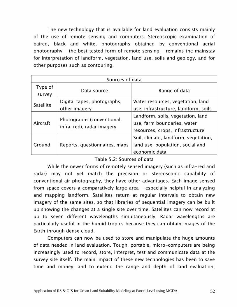
Application of RS & GIS for Urban Land Suitability Modeling at Parcel Level using MCDA 52
The new technology that is available for land evaluation consists mainly
of the use of remote sensing and computers. Stereoscopic examination of
paired, black and white, photographs obtained by conventional aerial
photography - the best tested form of remote sensing - remains the mainstay
for interpretation of landform, vegetation, land use, soils and geology, and for
other purposes such as contouring.
Sources of data
Type of
survey Data source Range of data
Satellite Digital tapes, photographs,
other imagery
Water resources, vegetation, land
use, infrastructure, landform, soils
Aircraft Photographs (conventional,
infra-red), radar imagery
Landform, soils, vegetation, land
use, farm boundaries, water
resources, crops, infrastructure
Ground Reports, questionnaires, maps
Soil, climate, landform, vegetation,
land use, population, social and
economic data
Table 5.2: Sources of data
While the newer forms of remotely sensed imagery (such as infra-red and
radar) may not yet match the precision or stereoscopic capability of
conventional air photography, they have other advantages. Each image sensed
from space covers a comparatively large area - especially helpful in analyzing
and mapping landform. Satellites return at regular intervals to obtain new
imagery of the same sites, so that libraries of sequential imagery can be built
up showing the changes at a single site over time. Satellites can now record at
up to seven different wavelengths simultaneously. Radar wavelengths are
particularly useful in the humid tropics because they can obtain images of the
Earth through dense cloud.
Computers can now be used to store and manipulate the huge amounts
of data needed in land evaluation. Tough, portable, micro-computers are being
increasingly used to record, store, interpret, test and communicate data at the
survey site itself. The main impact of these new technologies has been to save
time and money, and to extend the range and depth of land evaluation,

Application of RS & GIS for Urban Land Suitability Modeling at Parcel Level using MCDA 53
allowing data a greater complexity of land-use alternatives to be collected than
was possible in the past.
However, many kinds of data have to be collected in traditional ways. The
soil surveyor must dig or drill holes to describe the sequence of soil 'horizons'
with depth. The hydro-geologist may have to drill deeper holes to prove the
existence of suspected groundwater whilst hydrologists set up gauges on
streams to measure surface water flow. The meteorologist has to rely on
systematic measurements of change in the weather at established weather
stations. Agriculturalists, economists and sociologists observe people in action
in farms, villages and markets and, by means of questionnaires and other
enquiries, establish the patterns of their business. These and other scientists
collect the central core of basic data on land much as they have done for
decades.
• IdentiIdentiIdentiIdentifying lfying lfying lfying land useand useand useand usessss and their classification and their classification and their classification and their classification
---- D D D Definitions:efinitions:efinitions:efinitions:
The distinction between land cover and land use is fundamental. They are
defined as follows (Sims, 1995; De Bie, 1995):
‘Land cover is the observed physical cover, as seen from the ground or
through remote sensing, including the vegetation (natural or planted) and
human constructions (buildings, roads, etc.) which cover the earth's
surface. Water, ice, bare rock or sand surfaces are counted as land cover.’
‘Land use is based upon function, the purpose for which the land is being
used. Thus, a land use can be defined as a series of activities undertaken
to produce one or more goods or services. A given land use may take
place on one, or more than one piece of land, and several land uses may
occur on the same piece of land.’
Definition of land use in this way provides a basis for precise and
quantitative economic and environmental impact analysis, and permits precise
distinctions between land uses if required.

Application of RS & GIS for Urban Land Suitability Modeling at Parcel Level using MCDA 54
-Classification of land cover/land useClassification of land cover/land useClassification of land cover/land useClassification of land cover/land use::::
Classification is an abstract representation of the situation in the field
using well-defined diagnostic criteria, the classifiers. Sokal (1974) defined it as
"the ordering or arrangement of objects into groups or sets on the basis of
their relationships". A classification system describes the names of the classes
and the criteria used to distinguish them. A classification is, therefore, scale
independent and is independent of the means used to collect information
(whether satellite imagery, aerial photography or field survey or a combination
of them are used).
---- Classification structure: Classification structure: Classification structure: Classification structure:
- Hierarchical Systems: Hierarchical Systems: Hierarchical Systems: Hierarchical Systems:
Classification systems come in two basic formats, hierarchical or
non-hierarchical. A hierarchical classification offers more flexibility
because of its ability to accommodate different levels of
information, starting with structured broad-level classes which
allow further subdivision into more detailed sub-classes.
----Criteria for a (Reference) Land Cover Classification:Criteria for a (Reference) Land Cover Classification:Criteria for a (Reference) Land Cover Classification:Criteria for a (Reference) Land Cover Classification:
There are many classification systems in existence throughout the world.
However, there is no single internationally accepted land cover classification
system. Such a system should meet the criteria that:
- It must be comprehensive.
- It should be a common reference basis for all derived (and when
possible existing) classifications.
- It meets the needs of a variety of users (it should not be single project
oriented) which may take only part of the classification and develop from
there according to their own specific needs.
- it must be arranged in a hierarchical structure to be used at different
scales and at different levels of detail allowing cross-reference of local /
regional with continental/global maps without loss of information. Some
existing classifications are designed to be used at a specific scale and/or
consider only or mainly classes derived from satellite imagery.
- It must be able to describe all land cover features as derived from its
general definition.
- It must be adaptable to the variety of land cover types (all possible
combinations of the classifiers should be considered).

Application of RS & GIS for Urban Land Suitability Modeling at Parcel Level using MCDA 55
- A class must be defined by a combination of well-defined diagnostic
criteria, the classifiers. In most classifications there is an unclear or
unsystematic description of the classifiers from which the class should be
derived.
- Classes must be mutually exclusive and unambiguous.
- A clear distinction must exist between the types of classifiers used.
Often no underlying common principle has been identified and used to
define land cover. These factors influence land cover but are not inherent
features of it. This type of combinations are frequently applied in an
irregular way and often do not follow any hierarchy. This leads to
confusion in the final nomenclature.
- The diagnostic criteria or classifiers used in the classification must be
selected because of easy measurement and permanence.
- It should be suitable for mapping and monitoring purposes.
- It must be scientifically sound and practically oriented.
A primary source for the persistent use of “land use land cover”, or LULC,
is the so-called Anderson classification system, published by James Anderson
and colleagues in the 1976 USGS Professional Paper 1964. The Anderson
system formed the backbone of most land feature mapping done by the USGS
during the last three decades, although the classification schema has been
slightly altered over time. Land cover mapping is not standardized at present. It
is unlikely that it can be standardized at finer levels of detail given the vast
differences in the landscape across geographies, and the many different
purposes for which land feature mapping is required. The USGS has produced
several iterations of land cover and use maps for the continental U.S. that may
be considered as standard-setting.
The classification system used for NLCD is modified from the Anderson
land-use and land-cover classification system. Many of the Anderson classes,
especially the Level III classes, are best derived using aerial photography. It is
not appropriate to attempt to derive some of these classes using Landsat TM
data due to issues of spatial resolution and interpretability of data. Thus, no
attempt was made to derive classes that were extremely difficult or
“impractical” to obtain using Landsat TM data, such as the Level III urban
classes. In addition, some Anderson Level II classes were consolidated into a
single NLCD class.

Application of RS & GIS for Urban Land Suitability Modeling at Parcel Level using MCDA 56
- Similarities and differences between Anderson and NLCD systems Similarities and differences between Anderson and NLCD systems Similarities and differences between Anderson and NLCD systems Similarities and differences between Anderson and NLCD systems:
-Urban or builtUrban or builtUrban or builtUrban or built----up classes:up classes:up classes:up classes: Commercial, Industrial, Transportation,
and Communications/Utilities (all separate Anderson Level II
classes) were treated as one NLCD class (Commercial/Industrial/
Transportation). No attempt was made to derive Anderson Level III
classes in NLCD. “Recreational” grasses, such as those that occur in
golf courses or parks (treated as an urban class by Anderson) are
considered to be a non-urban class in NLCD (a subdivision of
“Herbaceous Planted/Cultivated). Residential (an Anderson Level II
class) was divided into Low and High Intensity classes in NLCD.
- Water:Water:Water:Water: Anderson Level II Water classes (Streams/Canals, Lakes/
Ponds, Reservoirs, Bays, Open Marine) were classed as a single
class (Open Water) in NLCD.
---- Agriculture: Agriculture: Agriculture: Agriculture: Agricultural areas that are herbaceous in nature
(Cropland and Pasture; Anderson Level II) are subdivided into four
NLCD classes: Pasture/Hay, Row Crops, Small Grains and Fallow.
---- Rangeland: Rangeland: Rangeland: Rangeland: No rangeland class (Anderson Level I) is identified by
NLCD. Rather, “rangeland” is subdivided by NLCD into
Grasslands/Herbaceous and Shrub land classes.
---- Forest land: Forest land: Forest land: Forest land: Evergreen Forest, Deciduous Forest and Mixed Forest
are the same in both Anderson and NLCD. Clear-cut and burned
areas are classed as “Transitional Bare” areas in NLCD.
---- Wetlands: Wetlands: Wetlands: Wetlands: Two classes are defined by NLCD. These are Woody
wetlands and Emergent/Herbaceous wetlands. These are very
analogous to the Anderson Level II wetland classes.
---- Bare: Bare: Bare: Bare: Three NLCD classes are recognized. These are: Bare
Rock/Sand Clay, Quarries/Strip Mines/Gravel Pits and Transitional
Bare. These represent a consolidation of Anderson Level II classes.
---- Tundra: Tundra: Tundra: Tundra: While “tundra” is treated as a distinct Anderson Level I
class, tundra (including arctic/alpine vegetation) is considered to
be either “Grasslands/Herbaceous” or “Shrub land” classes by
NLCD.

Application of RS & GIS for Urban Land Suitability Modeling at Parcel Level using MCDA 57
• Identifying environmental and socioIdentifying environmental and socioIdentifying environmental and socioIdentifying environmental and socio----economic issues:economic issues:economic issues:economic issues:
The land suitability not only is based on a set of physical parameters but
also very much dependent on the socioeconomic factors. Before a land use can
be recommended in a development plan, its environmental and socioeconomic
implications must be evaluated further. A new or improved land use can
succeed only if it can be adapted to fit local social and economic conditions.
Socio-economic investigations are therefore a vital part of land evaluation,
starting with the initial formulation of the study's objectives. Attention needs to
be given to markets (local, national and perhaps even international), population
levels and growth rates, the availability of skilled and unskilled labour,
transport of products and inputs, availability of building materials etc. Local
religions and cultures may be important. Political circumstances cannot be
ignored, and any analysis should take account of the needs of all members of
the population, including minority groups.
• Assessing suitability:Assessing suitability:Assessing suitability:Assessing suitability:
Suitability is a measure of how well the characteristics of a land match the
requirements of urban development. The preparation of urban development
plan requires consideration of all components of the environment that exist
before the new plan’s creation and the environment to be created by the new
development plan. The plan may not be effective if any of these components
are treated separately or loosely. Therefore the development plan should inter-
relate all elements that form a community. It is primarily because, the land is a
concrete form and any plan must be flexible enough to change established uses
either to correct mistakes or to accommodate changing needs. The steps that
are followed in the preparation of development plan proceeds from deciding
what land to develop to when and how to develop it. So the development plan
should encompass physical characteristics, constraints and socioeconomic
possibilities. Basically it refers to the potentiality of the land for the
development. Land potentiality includes both land suitability as well as land
value. The land suitability designates land according to its physical capability
regardless of any planner’s conceptual interest. The integration of land
suitability map and land value map produces a land potential map which can be
later combined with the socio-economic variables to prepare final alternative
development plan.
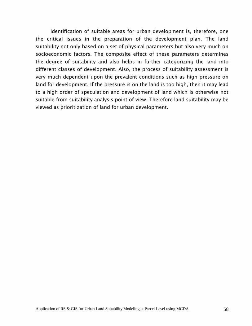
Application of RS & GIS for Urban Land Suitability Modeling at Parcel Level using MCDA 58
Identification of suitable areas for urban development is, therefore, one
the critical issues in the preparation of the development plan. The land
suitability not only based on a set of physical parameters but also very much on
socioeconomic factors. The composite effect of these parameters determines
the degree of suitability and also helps in further categorizing the land into
different classes of development. Also, the process of suitability assessment is
very much dependent upon the prevalent conditions such as high pressure on
land for development. If the pressure is on the land is too high, then it may lead
to a high order of speculation and development of land which is otherwise not
suitable from suitability analysis point of view. Therefore land suitability may be
viewed as prioritization of land for urban development.

Application of RS & GIS for Urban Land Suitability Modeling at Parcel Level using MCDA 59
Chapter 6: Study AreChapter 6: Study AreChapter 6: Study AreChapter 6: Study Area a a a ---- Bangalore Bangalore Bangalore Bangalore
• Introduction:Introduction:Introduction:Introduction:
The new Bangalore district came into existence from August 15th 1986
with the division of the erstwhile Bangalore district into Bangalore Rural and
Bangalore Urban districts. It is smallest among the districts of Karnataka State
with an area of about 2,191sqkm, but in population it stands first. Bangalore
district, as shown in Figure 6.1, has three taluks viz., Anekal, Bangalore North
and Bangalore South. The city is the headquarters of both the Bangalore Urban
and Bangalore Rural districts.
Figure 6.1: Location map of Bangalore City

Application of RS & GIS for Urban Land Suitability Modeling at Parcel Level using MCDA 60
• HHHHistoryistoryistoryistory::::
Several speculations have been made about how the name "Bangalore"
came about. Based on information from the Gazetteer of India, Karnataka State,
Bangalore District section, the name "Bangalore" is an anglicized version of
"Bengalooru," a word in the local Kannada language that was given to a town.
The story goes that this word was derived from the phrase "benda kaalu ooru,"
which translates into "the town of boiled beans". It is said that King Ballala of
the Hoysala dynasty lost his way in the jungle while on a hunting expedition.
Tired and hungry, he encountered a poor, old woman who offered him the only
food she had - some boiled beans. Grateful to her, the king named the place
"bende kaalu ooru." However, historical evidence shows that "Bengalooru" was
recorded much before King Ballala's time in a 9th century temple inscription in
the village of Begur. "Bengalooru" still exists today within the city limits in
Kodigehalli area and is called "Halebengalooru" or "Old Bangalore."
- Kempe Gowda Marks The Four Corners Of The City:Kempe Gowda Marks The Four Corners Of The City:Kempe Gowda Marks The Four Corners Of The City:Kempe Gowda Marks The Four Corners Of The City:
Another historical figure instrumental in shaping the city of Bangalore is a
feudal lord who called himself Kempe Gowda, and who served under the
Vijayanagara Kings. Hunting seemed to be a favorite past time in those days.
During one of his hunting bouts, Kempe Gowda was surprised to see a hare
chase his dog. Either his dog was chicken hearted or the hare was lion-hearted
one does not know, but the episode surely made an impression on the feudal
lord. He told himself this is a place surely for heroes and heroics, and he
referred to Bangalore from then onwards as "gandu bhoomi" (heroic place).
Kempe Gowda-I, who was in charge of Yelahanka, built a mud fort in 1537.
With the help of King Achutaraya, Kempe Gowda-I built the little towns of
Balepet, Cottonpet, and Chickpet, all inside the fort. Today, these little areas
serve as the major wholesale and commercial market places in the city. Kempe
Gowda's son's erected the four watch towers to mark the boundaries of
Bangalore which are traceable even today and they stand almost in the heart of
the present city. A hundred years later the Vijayanagara Empire fell, and in
1638, it was conquered by Mohammed Adil Shah, the Sultan of Bijapur.

Application of RS & GIS for Urban Land Suitability Modeling at Parcel Level using MCDA 61
---- Power Shifts from Sultans to Marathas to British: Power Shifts from Sultans to Marathas to British: Power Shifts from Sultans to Marathas to British: Power Shifts from Sultans to Marathas to British:
In 1638, Bangalore was conquered by Bijapur Sultan and ruled for next 50
years. Later it was captured by Mughals who held it for 3 years. In 1687, the
Mughal Sultan of Sira province sold Bangalore to king Chikkadevaraja Wodeyar
of Mysore for 3 lack pagodas, who built a second fort to the south of that built
by Kempegowda-I. In 1759, Hyder Ali received Bangalore as a jagir from
Krishna raja Wodeyar II. He fortified the southern fort and made Bangalore an
army town. When Tipu Sultan died in the 4th Mysore war in 1799, the British
gave the kingdom, including Bangalore back to Krishna raja Wodeyar III. The
British Resident stayed in Bangalore. In 1831, alleging misrule by Krishna raja
Wodeyar III, the British took over the administration of the Mysore Kingdom.
Under the British influence, Bangalore bloomed with modern facilities like the
railways, telegraphs, postal and police departments. In 1881, the British
returned the city to the Wodeyars. Diwans like Mirza Ismail, and sir
Vishweshwarayya were the pioneers to help Bangalore attain its modern
outlook. With the direct rule of the British Commissioners based in Bangalore, it
became the State Administrative HQ. The destiny of Bangalore thus took a
historic turn, making it eventually a major city of India and one of the fastest
growing in the world. After independence, Bangalore's choice as a state capital
was only logical. Mysore had too many associations with the royal family to be
the capital of a new state with an elected Chief Minister and a nominated
Governor. Finally, for an enlarged Karnataka, Bangalore was more central and
better linked with the major cities of the country.
---- Transformation of Bangalore City into Silicon Valley: Transformation of Bangalore City into Silicon Valley: Transformation of Bangalore City into Silicon Valley: Transformation of Bangalore City into Silicon Valley:
Today, Bangalore is booming, and a look at some of its nicknames says
why: "India's Silicon Valley," "Fashion Capital of India," "The Pub City of India,"
and so on. Home to well over 6.5 million people, and a base for 10,000
industries, Bangalore is India's fifth largest city and the fastest growing city in
Asia. The Bangalore has witnessed historical progression showing that workers
drifted from extractive agriculture to manufacturing and then services, followed
by a further shift to knowledge-based activities.
Lately, models of telematics-spurred information societies have been
forwarded as global phenomena that could spread to the entire world and usher
in sustainable development. Historically, Bangalore lacked major rivers running
around it or in the nearby environs. Artificial lakes or tanks were dug by the

Application of RS & GIS for Urban Land Suitability Modeling at Parcel Level using MCDA 62
city's kings to provide a water supply and support businesses, orchards,
military and administrative personnel. The defeat of the Vijayanagara Empire in
1565 swung trade routes and commercial activity in Bangalore's direction and
converted it into the leading economic locale in the Deccan plateau. Under Tipu
Sultan in the eighteenth century, the city experienced spurts in textiles,
metallurgy, ordnance and postal communications. British advent caused
industrial decline but made Bangalore a node within the colonial information
network, installing the first telegraph line in 1854. The city achieved a
reputation as a model princely state in the late colonial period. In 1898-9, it
had the first telephone lines in the country to coordinate anti-plague measures.
In 1900, it became India's first electrified city supplying power to run the Kolar
gold fields and steam textiles. M Visvesvarayya, the dynamic Diwan (chief
minister) of the Mysore kingdom from 1912 to 1918, flagged off major strides
for Bangalore in iron and steel, irrigation, education and engineering. He
imagined Bangalore as”science city" with "contributory facilities based on
information systems" as aids to trade at the time of India's independence, the
city had an emerging entrepreneurial and technological base. Being host to
public sector giants like Hindustan Aeronautics, Bharat Electronics and
Hindustan Machine Tools, Bangalore enjoyed a mushrooming of a range of
technical and service ancillaries in its conurbation. City planners followed
British city models and relocated factories from residential areas to distant
outskirts. Private businesses also expanded steadily due to the availability of
power, transportation and water. Prime Minister Jawaharlal Nehru took a
personal interest in Bangalore's profile as a scientific-industrial city. He saw it
as the "city of the future" and the "template of a modern India". By 1971, the
Bangalore metropolitan region supported a buoyant regional economy
attracting medium and small-scale industries. Corporate head offices fled the
left-wing militancy of Calcutta and settled in Bangalore, rewarding its liberal
industrial policy. As of 1991, the Bangalore region stood out among other
Indian cities for being an innovative haven, but "from a global perspective, it
was not an especially wealthy or healthy place". Dramatic unregulated growth of
the urban sprawl exceeded civic managerial capacity. All the major lakes
disappeared. Demand outstripped supply in housing and other major utilities.
More than 80% of newly built flats were being grabbed by land speculators,
pushing up real estate prices and slum populations. Environmentalists jabbed

Application of RS & GIS for Urban Land Suitability Modeling at Parcel Level using MCDA 63
at Bangalore as a "formerly model city". The cash-strapped state government
responded to this urban infrastructure crisis with the solution of partial
privatization. Geographic information systems were increasingly used to
superimpose spatial adjustments over existing maps in planning documents.
Computerized mapping and specialized consulting firms were hired by the
authorities to solve congestion and construction overkill. Equipped with
evolving technologies, planners drew new towns that could draw away
population from Bangalore as "counter magnets". Benchmarking programs
against the standards of Singapore, technocratic authorities pledged to deploy
the appropriate technology to enhance efficiency. It may be noted that a major
change in planning methodology evolved, wherein "centralized modes of
organization evolved into multi-entity networks constructed around electronic
information systems". The nature of the state was less "developmental" and
more in line with "coordinating" conditions for economic growth led by the
private sector. NGOs and citizen-based organizations were the other non-state
actors that played instrumental roles in the inter-organizational networks that
signified change in Bangalore. These "third force" groups strove for
decentralizing urban self-governance and involving the end-users of service
delivery in decision making about city amenities. Banking on the hypothesis
that information flows advance efficiency, they galvanized denizens for
participatory planning. Bangalore acquired an international reputation as India's
"Silicon Valley/Plateau" suddenly in the 1990s. But it was the denouement of
"the gradual accumulation of skills and capital since the beginning of the
twentieth century". The division of labor statistics in 1991 hardly fit the image
of a city with a milieu of innovation, with barely any Silicon Valley
characteristics. However, a series of state-engineered developments did
engender a niche within Bangalore's industrial economy that pushed technology
frontiers. Private enterprises like Wipro Infotech responded to Prime Minister
Rajiv Gandhi's electronics sector liberalization in 1984 and became one of the
city's first global successes. Infosys Consultants (later Technologies) bagged
software outsourcing and body-shopping agreements after Rajiv Gandhi's aides
facilitated a contract with General Electric in 1988. The success of these flag
bearers and USAID publications increased the interest of US technology
companies in Bangalore. Motorola, Oracle, Sun Microsystems and Hewlett
Packard established subsidiaries in the city, benefiting from its economic
Application of RS & GIS for Urban Land Suitability Modeling at Parcel Level using MCDA 64
liberalization policies. American companies were the largest group of foreign
investors fascinated by electronics and telematics in Bangalore. Software dove-
tailed with India's new export-oriented growth strategy and made up the most
positive contribution by Bangalore to the country's trade balance. The
Karnataka state government's interventions were also crucial in Bangalore's
leapfrogging technology curve. Besides launching the "Electronics City" complex
and building Software Technology Parks, it engaged in importuning propaganda
promoting Bangalore as a "Silicon Plateau" with themes like "the future is here".
Such marketing techniques intersected with a time of hyperbole and great
expectations for Indians trail blazing the fields of computers and
telecommunications. US commentators added fuel to fire by claiming that
"Bangalore has put together all the ingredients of a broad frontal attack on
American hegemony of the information revolution". But rising production costs
and infrastructure shortages emerged in the late 1990s and so did domestic
competitor cities like Pune and Hyderabad. Besides information technology,
several other ingredients determine Bangalore as an information society.
Bangalore urban district has an overall literacy rate of 86%. Bangalore University
boasts of 375 colleges that include 21 reputed engineering schools. The city is
home to 25,000 software and computer science engineers within an all-India
total of 220,000. In response to market demands for business-savvy techies,
the Indian Institute of Information Technology, Bangalore (IIIT-B) is churning
out batches of engineers who have undergone two terms of classes in industry
and corporate management. Bangalore's Indian Institute of Science (IISc) ranks
among the top 20 universities of the world. Its faculty members consult about
100 projects for industry every year. The availability of expert research
consultants and digitized databases are major causes for the clustering of New
Economy firms in the city. Bangalore also has a massive and pervasive print
culture, with 67 book publishers, 110 newspapers and countless specialized
magazines disseminating information to numerous social groups. A dense array
of film theaters makes the city an important source of visual information. More
than 80% of Bangaloreans own transistor radio sets, components of an
impressive electronic information system. Television broadcasting in India is
intertwined with the country's space program headquartered in Bangalore.
Cable and satellite penetration in the city is 59%. It has 1.6 million telephone
lines, one for every nine persons. Many cellular companies maintain
Application of RS & GIS for Urban Land Suitability Modeling at Parcel Level using MCDA 65
headquarters or technical offices in Bangalore. The Internet user population in
the city in 2001 stood at 80,000, emanating from 750 educational institutions.
Multinationals are benefiting from a vast increase in bandwidth for business
ends. It may be concluded that Bangalore "went online during a twenty-year
period" and "informatized" as a city. It can today be considered a regional
cluster within a global neo-liberal paradigm. This is both strength and
weakness, for worldwide booms and busts in IT and bio-informatics would
synchronize crests and troughs in Bangalore's economy. On the social front, the
application of hi-tech solutions has abetted transparency and popular
participation but also concentrated wealth and power in the hands of elites.
Digital democracy is a far cry in the network city. According to a study
conducted by the Confederation of Indian Industry (CII) and Karnataka's Vision
Group on Biotechnology, in 2001-02 there were 72 companies dealing in core
biotech areas employing over 5,000 people, of which 3,500 were scientists. The
total project investments were over Rs. 500 crores (1990-2001) with a total
venture capital funding of over Rs. 70 cores in the past two years, making a
total revenue of Rs. 700 crores, of which Rs. 250 crores came from exports. In
2002-03 there are about 100 biotech companies in Karnataka.
• Drainage:Drainage:Drainage:Drainage:
There are no major rivers flowing in the district. The Arkavati River flows
in the district for a small distance in Bangalore North taluk. The Dakshina
Pinakini touches and borders of the district to the north-east of the Anekal
taluk. The Vrishabhavati, a tributary of the Arkavati, flows in the district before
joining the Arkavati near Muduvadidurga. The tributary takes its birth in the
Bangalore city at Basavanagudi and the Suvarnamukhi from Anekal taluk joins
the tributary before joining the Arkavati. The Basavanahole originating beyond
the Muthyalamadu falls passes through Anekal taluk and joins the Arkavati near
Kanakapura. The western portion of Anekal taluk is marked by a continuous
chain of hills through which several rivulets combine together and drain into
the Arkavati. The rain water falling on eastern portions of the taluk drains into
the South Pinakini beyond the state boundary.

Application of RS & GIS for Urban Land Suitability Modeling at Parcel Level using MCDA 66
• Climate:Climate:Climate:Climate:
Bangalore is considered to be climatically a well favored district situated
in the heart of South Deccan of Peninsular India. The climate of the district is
classed as the seasonally dry tropical savanna climate with four seasons.
- The dry season with clear bright weather is from December to
February.
- The summer season from March to May
- The South-west monsoon season from June to September.
- The post monsoon season starts from October and November.
On the basis of mean monthly temperatures, April is usually the hottest
month with the mean daily maximum temperature at 33.4°C and the mean daily
minimum at 21.2° C. on individual days, in hot season, the day temperatures
often go above 36° C. With the onset of the monsoon early in June, there is
appreciable drop in the day temperatures but that in night temperature is only
slight. In October, the temperatures are as in the south-west monsoon season.
Thereafter, temperatures decrease. December is generally the coolest month
with the mean daily maximum temperature at 25.7° C and the mean daily
minimum at 15.3° C Nights during January are however slightly colder than
during December.
The mean monthly relative humidity is the lowest in the month of March
and humidity is high during the period June of October, i.e., between 80% to
85% on the average. Humidity decreases thereafter and the period February to
April, the air is comparatively drier, the afternoon relative humidity being 25%
to 35%.
• Rainfall:Rainfall:Rainfall:Rainfall:
The average annual rainfall of Bangalore urban district is 751.6 mm and
the mean number of rainy days is about 57. Bangalore has three different rainy
periods covering eight months of the year followed closely one after the other.
Of these, June to September is the principal rainy season. Bangalore receives
54% of the total annual rainfall in the south-west monsoon period, 36% of the
annual rainfall during north east monsoon. Thus 80 percent of the annual rain
falls during the six months June to November Remaining 20 percent of the
rainfall during April and May. December to March is comparatively rainless
period, with a mean rainfall of 33 mm and about 3 to 4 rainy days. The details
of the rainfall for each taluk are given in the following Table 6.1.

Application of RS & GIS for Urban Land Suitability Modeling at Parcel Level using MCDA 67
District Name of the
taluk
Average annual rain fall in
mm
Bangalore North 789.03
Bangalore South 722.48 Bangalore urban
Anekal 737.35
Table 6.1: Rainfall in Bangalore Urban District
• Geology:Geology:Geology:Geology:
The entire Anekal taluk is composed of only one type of rock called
gneissic granites belonging to Precambrian age. These rocks are exposed as a
continuous chain of mounds raising 90 to 150 meters above the general
ground level on the western portion of the taluk. These form the Bannerghatta
group of hills. Rocky outcrops are few and far between the middle and eastern
portions of the taluk. Inclusions of quartz and pegmatite veins are common.
The depth of weathering varies greatly. The central and eastern portions of the
taluk show maximum thickness of the weathered mantle, extending to more
than 12 meters. The western portion of the taluk is deeply dissected and rocky.
The chief rock types occurring in Bangalore North taluk are granites and
gneisses. These are prominently exposed as a ridge running NNE and SSW
almost in the middle of the taluk. The granitic gneisses are crisscrossed by
Pegmatitic and Aplitic veins. Basic Xenolithic patches are common. Banding is
prominent. The rocks are highly jointed, and sheet jointing parallel to the
exposed surface is particularly characteristic of the Bangalore gneisses.
Granites and gneisses are intruded by a number of basic dykes. Dykes are
oriented east-west and as well as north-south. Cappings of laterites are found
at the highest point in Bangalore, beneath the laterite, the gneisses are deeply
weathered giving into various shades of clay. These exposures are well seen
near Yelahanka and neighborhood.
Bangalore south taluk comprises granites and granitic gneisses belonging
to Pre-Cambrian age. The granitic gneisses are exposed as continuous chains
of mounds raising 30 to 70 meters above ground level in the southern region of
the taluk. Granites are medium to coarse grained hard, compact and massive.
Granitic gneisses are distinctly banded and are in various shades of grey color.
The strike of foliation is usually NNW-SSE. They are traversed by Pegmatitic and
aplitic veins. Sheet jointing is very common. Granites and gneisses have

Application of RS & GIS for Urban Land Suitability Modeling at Parcel Level using MCDA 68
undergone different degree of alteration and decomposition. Southern and
eastern regions of the taluk show maximum thickness of weathered mantle
extending up to about 20 meters while the depth of the weathered zone is
maximum generally in the valleys, in highly cut-up terrain, as in the southern
parts of the taluk. Granites and granitic gneisses are traversed by vertical and
horizontal joints and are intruded by dolerite dykes.
• Demography:Demography:Demography:Demography:
The population of Bangalore has had exponentially increased from a mere
7.64 lakhs in 1950 to 65.33 lakhs in 2005. Over a span of 55 years the
population has increased by 57.69 with an average decadal growth of 10.49
lakhs. The reasons for the fastest growth in population may be attributed to
dynamic transformation of Bangalore from industrial city to educational city,
educational city to health city, from health city to IT city and so on and also the
optimal weather conditions and cosmopolitan environment including the
generosity and hospitality of the local kannadigas.
Year Bangalore Population
1950 - 2015
Percentage of Indian
urban population (%)
1950 - 2015
Percentage of
total Indian population (%)
1950 - 2015
1950 764 000 1.2 0.2
1955 947 000 1.4 0.2
1960 1 173 000 1.5 0.3
1965 1 382 000 1.5 0.3
1970 1 616 000 1.5 0.3
1975 2 111 000 1.6 0.3
1980 2 812 000 1.8 0.4
1985 3 395 000 1.8 0.4
1990 4 036 000 1.9 0.5
1995 4 745 000 1.9 0.5
2000 5 567 000 2.0 0.6
2005 6 533 000 2.1 0.6
2010 7 469 000* 2.1 0.6
2015 8 391 000* 2.1 0.7
* Projected Population Source: UN 2005
Table 6.2: Population of Bangalore from 1950 to 2015

Application of RS & GIS for Urban Land Suitability Modeling at Parcel Level using MCDA 69
There are 100 wards within the Bangalore Mahanagara Palike (BMP) limits.
The population statistics as per census 2001 is as given the following Table
6.3. covering 100 BMP wards and 08 CMC’s excluding the new layouts being
developed and not handed over to either BMP or CMC.
Bangalore Wards / CMC Population as per census 2001
Bangalore (M Corp.) - Ward No.1 27637
Bangalore (M Corp.) - Ward No.2 36125
Bangalore (M Corp.) - Ward No.3 46677
Bangalore (M Corp.) - Ward No.4 54704
Bangalore (M Corp.) - Ward No.5 36287
Bangalore (M Corp.) - Ward No.6 38723
Bangalore (M Corp.) - Ward No.7 37760
Bangalore (M Corp.) - Ward No.8 40673
Bangalore (M Corp.) - Ward No.9 38905
Bangalore (M Corp.) - Ward No.10 34702
Bangalore (M Corp.) - Ward No.11 35403
Bangalore (M Corp.) - Ward No.12 43445
Bangalore (M Corp.) - Ward No.13 38743
Bangalore (M Corp.) - Ward No.14 36918
Bangalore (M Corp.) - Ward No.15 37005
Bangalore (M Corp.) - Ward No.16 61314
Bangalore (M Corp.) - Ward No.17 29275
Bangalore (M Corp.) - Ward No.18 25742
Bangalore (M Corp.) - Ward No.19 23228
Bangalore (M Corp.) - Ward No.20 28121
Bangalore (M Corp.) - Ward No.21 47682
Bangalore (M Corp.) - Ward No.22 41471
Bangalore (M Corp.) - Ward No.23 35465
Bangalore (M Corp.) - Ward No.24 34595
Bangalore (M Corp.) - Ward No.25 35411
Bangalore (M Corp.) - Ward No.26 37507
Bangalore (M Corp.) - Ward No.27 32809
Bangalore (M Corp.) - Ward No.28 31851
Bangalore (M Corp.) - Ward No.29 40704
Bangalore (M Corp.) - Ward No.30 39521

Application of RS & GIS for Urban Land Suitability Modeling at Parcel Level using MCDA 70
Bangalore Wards / CMC Population as per census 2001
Bangalore (M Corp.) - Ward No.31 28069
Bangalore (M Corp.) - Ward No.32 40047
Bangalore (M Corp.) - Ward No.33 40867
Bangalore (M Corp.) - Ward No.34 44368
Bangalore (M Corp.) - Ward No.35 40131
Bangalore (M Corp.) - Ward No.36 56340
Bangalore (M Corp.) - Ward No.37 21896
Bangalore (M Corp.) - Ward No.38 15597
Bangalore (M Corp.) - Ward No.39 40478
Bangalore (M Corp.) - Ward No.40 25619
Bangalore (M Corp.) - Ward No.41 51746
Bangalore (M Corp.) - Ward No.42 43223
Bangalore (M Corp.) - Ward No.43 59933
Bangalore (M Corp.) - Ward No.44 43892
Bangalore (M Corp.) - Ward No.45 40821
Bangalore (M Corp.) - Ward No.46 40725
Bangalore (M Corp.) - Ward No.47 32938
Bangalore (M Corp.) - Ward No.48 42919
Bangalore (M Corp.) - Ward No.49 41075
Bangalore (M Corp.) - Ward No.50 31893
Bangalore (M Corp.) - Ward No.51 39484
Bangalore (M Corp.) - Ward No.52 35660
Bangalore (M Corp.) - Ward No.53 62163
Bangalore (M Corp.) - Ward No.54 82630
Bangalore (M Corp.) - Ward No.55 112407
Bangalore (M Corp.) - Ward No.56 87307
Bangalore (M Corp.) - Ward No.57 63906
Bangalore (M Corp.) - Ward No.58 40430
Bangalore (M Corp.) - Ward No.59 34613
Bangalore (M Corp.) - Ward No.60 39308
Bangalore (M Corp.) - Ward No.61 39505
Bangalore (M Corp.) - Ward No.62 53934
Bangalore (M Corp.) - Ward No.63 48979

Application of RS & GIS for Urban Land Suitability Modeling at Parcel Level using MCDA 71
Bangalore Wards / CMC Population as per census 2001
Bangalore (M Corp.) - Ward No.64 63111
Bangalore (M Corp.) - Ward No.65 51545
Bangalore (M Corp.) - Ward No.66 65820
Bangalore (M Corp.) - Ward No.67 45929
Bangalore (M Corp.) - Ward No.68 40986
Bangalore (M Corp.) - Ward No.69 52079
Bangalore (M Corp.) - Ward No.70 34682
Bangalore (M Corp.) - Ward No.71 39790
Bangalore (M Corp.) - Ward No.72 44357
Bangalore (M Corp.) - Ward No.73 42288
Bangalore Wards / CMC Population as per census 2001
Bangalore (M Corp.) - Ward No.74 39820
Bangalore (M Corp.) - Ward No.75 36035
Bangalore (M Corp.) - Ward No.76 36465
Bangalore (M Corp.) - Ward No.77 32451
Bangalore (M Corp.) - Ward No.78 37028
Bangalore (M Corp.) - Ward No.79 34988
Bangalore (M Corp.) - Ward No.80 35681
Bangalore (M Corp.) - Ward No.81 39669
Bangalore (M Corp.) - Ward No.82 33359
Bangalore (M Corp.) - Ward No.83 50256
Bangalore (M Corp.) - Ward No.84 31985
Bangalore (M Corp.) - Ward No.85 34943
Bangalore (M Corp.) - Ward No.86 39586
Bangalore (M Corp.) - Ward No.87 56530
Bangalore (M Corp.) - Ward No.88 26103
Bangalore (M Corp.) - Ward No.89 32889
Bangalore (M Corp.) - Ward No.90 43432
Bangalore (M Corp.) - Ward No.91 42078
Bangalore (M Corp.) - Ward No.92 39663
Bangalore (M Corp.) - Ward No.93 51578
Bangalore (M Corp.) - Ward No.94 60896
Bangalore (M Corp.) - Ward No.95 84461

Application of RS & GIS for Urban Land Suitability Modeling at Parcel Level using MCDA 72
Bangalore Wards / CMC Population as per census 2001
Bangalore (M Corp.) - Ward No.96 74126
Bangalore (M Corp.) - Ward No.97 38042
Bangalore (M Corp.) - Ward No.98 52546
Bangalore (M Corp.) - Ward No.99 32560
Bangalore (M Corp.) - Ward No.100 52263
Pattanagere (CMC+OG) 96385
Dasarahalli (CMC+OG) 293359
Yelahanka (CMC+OG) 94234
Byatarayanapura (CMC+OG) (Part) 188514
Kengeri (TMC) 42455
Krishnarajapura (CMC) 186210
Mahadevapura (CMC+OG) 154223
Bommanahalli (CMC+OG) (Part) 224980
TOTAL 5581686
Table 6.3: Ward / CMC- wise Population as per census 2001

Application of RS & GIS for Urban Land Suitability Modeling at Parcel Level using MCDA 73
• Population Distribution:Population Distribution:Population Distribution:Population Distribution:
As per census 2001, the distribution of population in northern, southern
and south-eastern wards in dark brown coloured wards (ref: Figure 6.5) is more
han 60,000. The population in western and eastern parts is relatively less.
Figure 6.5: Population distribution in BMP wards
• Location of study area:Location of study area:Location of study area:Location of study area:
The study area for the project work has been restricted to only
29 villages out of 865 villages within the Bangalore urban district
keeping in mind the constraint of manpower and time required.
These contigous29 villages are located in south-eastern part of
Bangalore city as shown in Figure 6.2. The likely landuse plan for
these parcels and the surrounding villages as depicted in Master
Plan (2005-2015) proposed by the Bangalore Development
Authority is shown as in Figure 6.3. Also the location of study area
with respect to the administrative boundary of the statutory agency
for Bangalore urban development, the Bangalore Development
Authority is shown in Figure 6.3.

Application of RS & GIS for Urban Land Suitability Modeling at Parcel Level using MCDA 74
Chapter 7: The Methodology and Data Base CreationChapter 7: The Methodology and Data Base CreationChapter 7: The Methodology and Data Base CreationChapter 7: The Methodology and Data Base Creation
• Introduction:Introduction:Introduction:Introduction:
The overall methodology adopted for site suitability analysis for urban
development is given in the Figure 7.1. Various important factors relevant for
Bangalore such as present landuse/landcover, proximity to existing road
network, proximity to the built-up, soil depth, soil texture, ground water
prospects and land value are chosen so as to keep the model compact and
effective. These factor vector layers are weighted according to the weights
derived by the Saaty’s AHP method by creating a separate field in each layer.
Each class or category in each layer is given rank and these ranks are stored in
the database as separate field. And also the product of weight and rank are
computed and stored in another filed. Finally all the seven factor vector layers
are combined together by applying GIS UNION operation on two layers at a
time. Thus totally six UNION operations are carried out to seven factor vector
layers to get the final weighted combined factor vector layer. Similarly, three
constraints such as built-up area, water bodies and master plan are considered.
These three constraint vector layers are combined together by applying Boolean
AND operation on two layers at a time. Finally, the constraint combined vector
map is obtained by applying two Boolean AND operations on constraint layers.
Ultimately the INTERSECTION of the factor map and the constraint map give the
site suitability for urban development. The final parcel level urban land
suitability map is obtained by INTERSECTION of urban land suitability map and
the cadastral layer being created by onscreen digitization on the mosaiced
cadastral maps being geo-referenced over the merged Quickbird satellite
image. The vector layers are used to achieve maximum accuracy keeping in
mind the parcel level land suitability analysis.
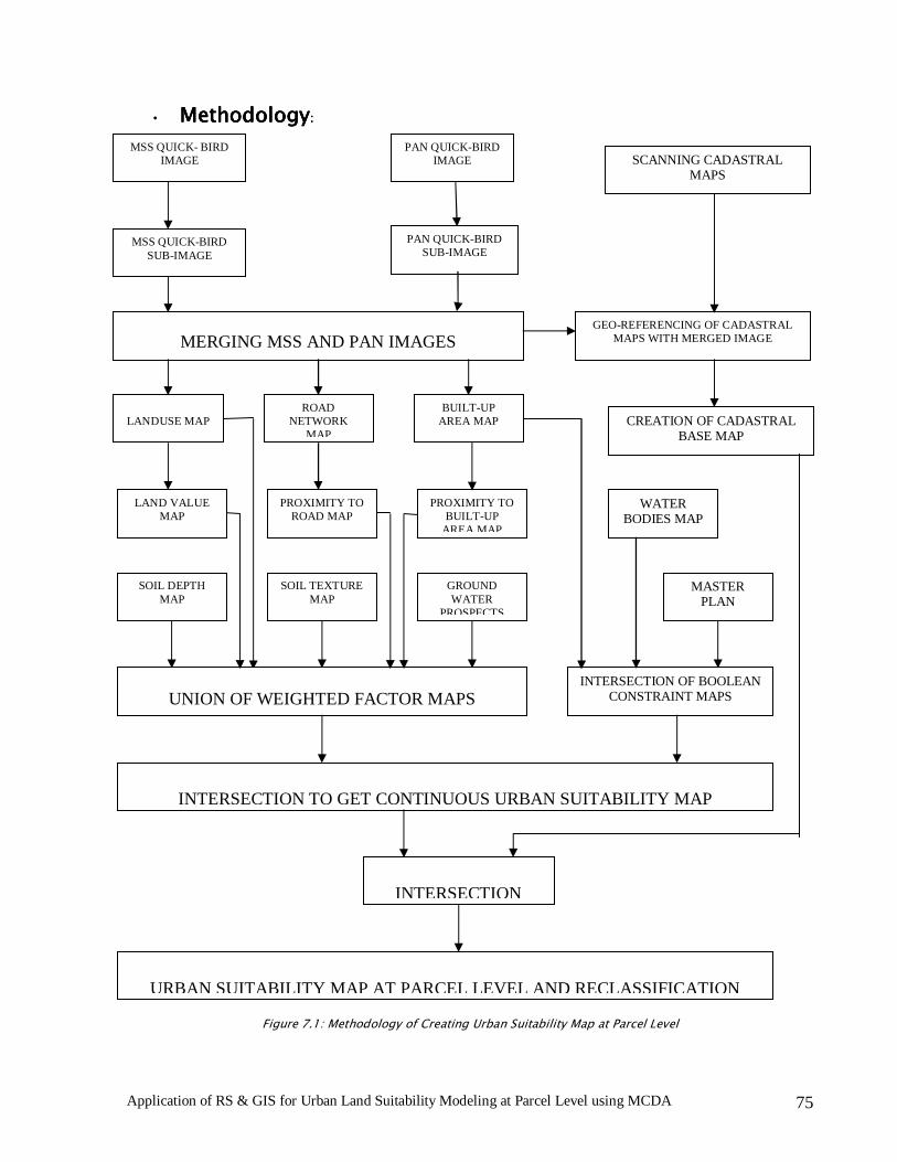
Application of RS & GIS for Urban Land Suitability Modeling at Parcel Level using MCDA 75
• MethodologyMethodologyMethodologyMethodology::::
Figure 7.1: Methodology of Creating Urban Suitability Map at Parcel Level
LANDUSE MAP
MSS QUICK-BIRD SUB-IMAGE
PAN QUICK-BIRD SUB-IMAGE
MERGING MSS AND PAN IMAGES
PAN QUICK-BIRD IMAGE
ROAD NETWORK
MAP
BUILT-UP AREA MAP
LAND VALUE MAP
PROXIMITY TO ROAD MAP
PROXIMITY TO BUILT-UP
AREA MAP
SOIL DEPTH MAP
SOIL TEXTURE MAP
GROUND WATER
PROSPECTS
MSS QUICK- BIRD IMAGE
UNION OF WEIGHTED FACTOR MAPS
GEO-REFERENCING OF CADASTRAL MAPS WITH MERGED IMAGE
SCANNING CADASTRAL MAPS
INTERSECTION OF BOOLEAN CONSTRAINT MAPS
WATER BODIES MAP
MASTER PLAN
CREATION OF CADASTRAL BASE MAP
INTERSECTION TO GET CONTINUOUS URBAN SUITABILITY MAP
INTERSECTION
URBAN SUITABILITY MAP AT PARCEL LEVEL AND RECLASSIFICATION

Application of RS & GIS for Urban Land Suitability Modeling at Parcel Level using MCDA 76
• Factors:Factors:Factors:Factors:
They are the additive layers which are unioned to arrive at most favorable
areas for urban development in terms of higher attribute values.
---- Existing landuse landcover classifica Existing landuse landcover classifica Existing landuse landcover classifica Existing landuse landcover classification:tion:tion:tion:
---- Introduction: Introduction: Introduction: Introduction:
Information on existing landuse/cover (refer to Figure 7.3)
especially the extent and spatial distribution is a prerequisite for the
urban suitability studies or urban planning. Up-to-date landuse /
landcover map is required for monitoring the urban and rural
environment. Landuse refers to man’s activities and the various use which
they are put whereas landcover refers to the natural vegetation, water
bodies, rock/soil, artificial cover and others resulting due to land
transformations. Landuse is generally based on landcover. Landuse
encompasses several different aspects of man’s relationship to the
environment e.g., activity, ownership and land quality. Landcover is
represented by natural and artificial compositions covering the earth’s
surface at certain location e.g., building as cover for residential use,
green plants as a cover for agricultural crop.
---- Classification system adopted Classification system adopted Classification system adopted Classification system adopted
The classification system adopted in this study is developed
keeping in mind the following objectives.
- To demonstrate the technique used and its advantage in
obtaining information for urban area
-Utilization of VHR satellite data (refer to Figure 7.2) for
identification, mapping and classification of various landuses
in detail.
---- Built Built Built Built----up land:up land:up land:up land:
The physical extent of total built-up or developed land is about
1331.031331.031331.031331.03 hectares in the study area.
---- Agricultural land: Agricultural land: Agricultural land: Agricultural land:
Agriculture is the predominant landuse outside the urban area. The
area covered under agricultural landuse is about 2447.422447.422447.422447.42 hectares. The

Application of RS & GIS for Urban Land Suitability Modeling at Parcel Level using MCDA 77
agricultural land includes crop land, fallow land, water logged area. The
types of crops grown in the study area are mostly ragi, rice, fruits and
vegetables.
---- Plantations: Plantations: Plantations: Plantations:
The area under plantations is about 1510.761510.761510.761510.76 hectares. Mostly
plantations include eucalyptus, coconut and areca nut plantations.
---- Waste land: Waste land: Waste land: Waste land:
The area under vacant land is about hectares 420.35420.35420.35420.35 hectares. It
covers non-irrigable land, open spaces, scrubs.
---- Water bodies: Water bodies: Water bodies: Water bodies:
The total area under water bodies is about 429.32429.32429.32429.32 hectares. The
prime water body is the bellandur amanikere with a series of
interconnected tanks. Most of these tanks feed for paddy crop.
---- Transportation network: Transportation network: Transportation network: Transportation network:
The road network is one of the important parameter in identifying
the areas for urban development as it provides linkages between the
settlements. The major and minor pucca roads have considered for
digitization.
Sl NoSl NoSl NoSl No Landuse TypeLanduse TypeLanduse TypeLanduse Type Area(Ha)Area(Ha)Area(Ha)Area(Ha)
1 Built-Up 1331
2 Agriculture 2447
3 Plantation 1511
4 Transport 30
5 Waste Land 420
6 Water Bodies 429
TotalTotalTotalTotal 6666169169169169 Table 7.1: Areas of Landuse/Landcover Classes in the study areaTable 7.1: Areas of Landuse/Landcover Classes in the study areaTable 7.1: Areas of Landuse/Landcover Classes in the study areaTable 7.1: Areas of Landuse/Landcover Classes in the study area
---- Ground Water Prospects: Ground Water Prospects: Ground Water Prospects: Ground Water Prospects:
Geomorphic features control the distribution of runoff and ground water
recharge. The structure of geological formation controls the occurrence,
movement and quality of ground water. Primary importance is the occurrence

Application of RS & GIS for Urban Land Suitability Modeling at Parcel Level using MCDA 78
and distribution of aquifers and their relationship with relatively associated
impermeable beds, which act as non-leaky to leaky confining layers and
barriers to ground water movement. The geological structures have marked
influence on the lateral and vertical extent of aquifers.
Existing hydro-geo-morphological map (scale: 1:50000) being prepared
by KSRSAC, Bangalore on the basis of geology, geomorphology and structure
has been used for extracting ground water prospects map (refer to Figure 7.4).
Hydro-morphologically, the study area has been divided into five zones
depending upon the ground water prospects in different geomorphic units.
These five zones are i) Very good, ii) Good, iii) Moderate, iv) Poor, v) nil
Alluvial plains are very good potential zones. Ground water occurs under
water table condition between 8 M to 20 M but deeper level due to presence of
loose fragmented material supports high value of permeability and more
chance of downward percolation of surface water. In valley fill and in-filled
valley area, the ground water prospects are mainly dependent on the thickness
of the weathered and colluvial soil. Therefore these areas have good ground
water prospects.
Sl NoSl NoSl NoSl No Ground Water ProspGround Water ProspGround Water ProspGround Water Prospectsectsectsects Area(Ha)Area(Ha)Area(Ha)Area(Ha)
1 Good 1473
2 Moderate 4381
3 Moderate to Poor 21
4 Reservoir 295
TotalTotalTotalTotal 6169616961696169 Table 7.2: Areas of Ground Water prospects Classes in the study areaTable 7.2: Areas of Ground Water prospects Classes in the study areaTable 7.2: Areas of Ground Water prospects Classes in the study areaTable 7.2: Areas of Ground Water prospects Classes in the study area
---- Soil Information: Soil Information: Soil Information: Soil Information:
The soil map prepared by KSRSAC, Bangalore in the scale of 1:50000, is
being used for extracting the soil depth and soil texture layers. Each polygon
has the information related to the association of soil series. From these soil
types, soil depth and soil texture have been separated out and the maps have
been prepared separately. The extent and spatial distribution of soil depth and
soil texture play an important role in urban suitability analysis.

Application of RS & GIS for Urban Land Suitability Modeling at Parcel Level using MCDA 79
---- Soil depth: Soil depth: Soil depth: Soil depth:
As per IS Building code the minimum depth of foundation within soil
should not be less than 45 cm for buildings. Therefore the soil depths are
categorized into three classes (refer to Figure 7.5). They are i) deep (depth >90
cm), ii) moderately deep (depth >45 cm to depth < 90 cm), iii) shallow (depth <
45 cm).
SlSlSlSl No No No No Soil DepthSoil DepthSoil DepthSoil Depth Area(Ha)Area(Ha)Area(Ha)Area(Ha)
1 Deep 3274
2 Moderately Deep 1048
3 Shallow 1848
TotalTotalTotalTotal 6169616961696169
Table 7.3: Areas of Soil Depth Classes in the study areaTable 7.3: Areas of Soil Depth Classes in the study areaTable 7.3: Areas of Soil Depth Classes in the study areaTable 7.3: Areas of Soil Depth Classes in the study area
---- Soil texture Soil texture Soil texture Soil texture
It is an important aspect with respect to the stability of foundations.
Clayey soils increase in volume due to absorption of water and may result in
differential settlement of foundations resulting in their failure. Therefore, highly
clayey soils are less suitable and sandy soils are more suitable for foundations.
According to the texture of soils five categories are made as follows (refer to
Figure 7.6). i) Settlement/Tank/Gullied land (not suitable), ii) Clay /Clay loam
(less suitable), iii) Sandy clay (moderately suitable), iv) Gravelly clay (suitable)
and v) Sandy loam/loamy sand (highly suitable).
SlSlSlSl No No No No Soil TextureSoil TextureSoil TextureSoil Texture Area(Ha)Area(Ha)Area(Ha)Area(Ha)
1 Clay 2203
2 Clay loam 21
3 Gravelly clay 1026
4 Gullied land 3
5 Loamy sand 14
6 Sandy clay 1155
7 Sandy loam 723
8 Settlement 729
9 Tank 294
TotalTotalTotalTotal 6169616961696169
Table 7.4: Areas of Soil Texture Classes in the study areaTable 7.4: Areas of Soil Texture Classes in the study areaTable 7.4: Areas of Soil Texture Classes in the study areaTable 7.4: Areas of Soil Texture Classes in the study area
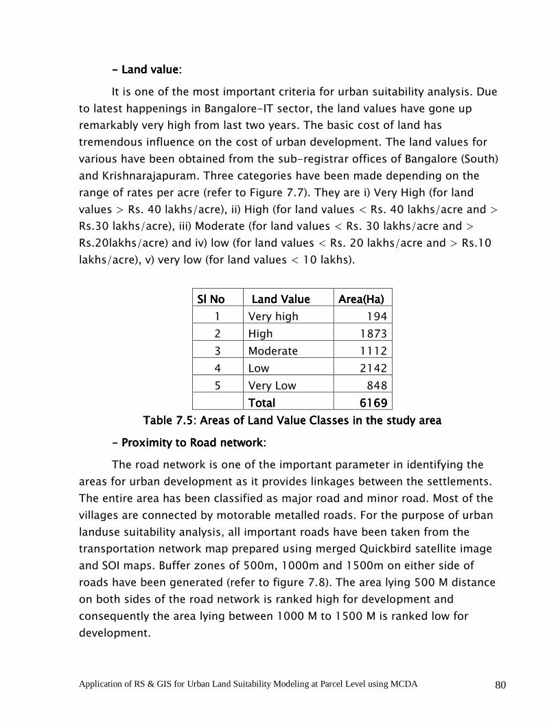
Application of RS & GIS for Urban Land Suitability Modeling at Parcel Level using MCDA 80
---- Land value: Land value: Land value: Land value:
It is one of the most important criteria for urban suitability analysis. Due
to latest happenings in Bangalore-IT sector, the land values have gone up
remarkably very high from last two years. The basic cost of land has
tremendous influence on the cost of urban development. The land values for
various have been obtained from the sub-registrar offices of Bangalore (South)
and Krishnarajapuram. Three categories have been made depending on the
range of rates per acre (refer to Figure 7.7). They are i) Very High (for land
values > Rs. 40 lakhs/acre), ii) High (for land values < Rs. 40 lakhs/acre and >
Rs.30 lakhs/acre), iii) Moderate (for land values < Rs. 30 lakhs/acre and >
Rs.20lakhs/acre) and iv) low (for land values < Rs. 20 lakhs/acre and > Rs.10
lakhs/acre), v) very low (for land values < 10 lakhs).
SlSlSlSl No No No No Land ValueLand ValueLand ValueLand Value Area(Ha)Area(Ha)Area(Ha)Area(Ha)
1 Very high 194
2 High 1873
3 Moderate 1112
4 Low 2142
5 Very Low 848
TotalTotalTotalTotal 6169616961696169
Table 7.5: Areas of Land Value Classes in the study areaTable 7.5: Areas of Land Value Classes in the study areaTable 7.5: Areas of Land Value Classes in the study areaTable 7.5: Areas of Land Value Classes in the study area
---- Proximity to Road network: Proximity to Road network: Proximity to Road network: Proximity to Road network:
The road network is one of the important parameter in identifying the
areas for urban development as it provides linkages between the settlements.
The entire area has been classified as major road and minor road. Most of the
villages are connected by motorable metalled roads. For the purpose of urban
landuse suitability analysis, all important roads have been taken from the
transportation network map prepared using merged Quickbird satellite image
and SOI maps. Buffer zones of 500m, 1000m and 1500m on either side of
roads have been generated (refer to figure 7.8). The area lying 500 M distance
on both sides of the road network is ranked high for development and
consequently the area lying between 1000 M to 1500 M is ranked low for
development.

Application of RS & GIS for Urban Land Suitability Modeling at Parcel Level using MCDA 81
SlSlSlSl No No No No Road BufferRoad BufferRoad BufferRoad Buffer Area(Ha)Area(Ha)Area(Ha)Area(Ha)
1 500 M 5172
2 1000 M 996
3 1500 M 0
TotalTotalTotalTotal 6169616961696169 Table 7.6: Areas of Proximity to Road Classes in the study areaTable 7.6: Areas of Proximity to Road Classes in the study areaTable 7.6: Areas of Proximity to Road Classes in the study areaTable 7.6: Areas of Proximity to Road Classes in the study area
---- Proximity to Built Proximity to Built Proximity to Built Proximity to Built----up area:up area:up area:up area:
It is considered due to the reason that the cost of future urban
development depends on proximity to the built-up area. A buffer of 500 M is
normally considered in urban development studies. Therefore, areas within 500
M buffer radius are more suitable for urban development than areas outside
500 M buffer limit (refer to Figure 7.9).
SlSlSlSl No No No No Built BufferBuilt BufferBuilt BufferBuilt Buffer Area(Ha)Area(Ha)Area(Ha)Area(Ha)
1 <500M 5419
2 >500M 750
TotalTotalTotalTotal 6169616961696169
Table 7.7: Areas of Proximity to BuiltTable 7.7: Areas of Proximity to BuiltTable 7.7: Areas of Proximity to BuiltTable 7.7: Areas of Proximity to Built----up Classes in the study areaup Classes in the study areaup Classes in the study areaup Classes in the study area
• Constraints:Constraints:Constraints:Constraints:
These are the layers which restrict the growth or urban development. Master
plan, water body and urban area are identified as important constraints for
urban development.
---- Master plan: Master plan: Master plan: Master plan:
Bangalore Development Authority (BDA) is an agency constituted in 1976
for regulating and monitoring the orderly growth of the Bangalore city. Recently
BDA released the Draft Master Plan - 2015 covering a Local Planning Area (LPA)
of 1306 sqkm. The BDA planning area consists of 387 villages, 7 City Municipal
Councils (CMC) and 1 Town Municipal Council (TMC). The areas classified under
‘Constraint Areas Category’ (CAC) within the LPA are restricted from
development. These Non-buildable areas have been extracted from the
Bangalore Master Plan (2005 – 2015) as shown in Figure 7.10. These areas are
mainly the low lying or valley areas prone to submerging during heavy rains.
The total non-buildable area in the study area is 89.24 hectares.

Application of RS & GIS for Urban Land Suitability Modeling at Parcel Level using MCDA 82
SlSlSlSl No No No No Master Plan ConstraintMaster Plan ConstraintMaster Plan ConstraintMaster Plan Constraint Area(Ha)Area(Ha)Area(Ha)Area(Ha)
1 Buildable 4543
2 Non-Buildable 1626
TotalTotalTotalTotal 6169616961696169 Table 7.8: Areas of Constraint (Master Plan) Classes in the study areaTable 7.8: Areas of Constraint (Master Plan) Classes in the study areaTable 7.8: Areas of Constraint (Master Plan) Classes in the study areaTable 7.8: Areas of Constraint (Master Plan) Classes in the study area
---- Built Built Built Built----up area:up area:up area:up area:
Obviously urban development can not take place in the developed area
(refer to Figure 7.11). Total built-up area is about 1331.03 hectares.
SlSlSlSl No No No No ClassClassClassClass Area(Ha)Area(Ha)Area(Ha)Area(Ha)
1 Built Up 1355
2 Others 4814
TotalTotalTotalTotal 6169616961696169 Table 7.9: Areas of Constraint (BuiltTable 7.9: Areas of Constraint (BuiltTable 7.9: Areas of Constraint (BuiltTable 7.9: Areas of Constraint (Built----up) Classes in the study areaup) Classes in the study areaup) Classes in the study areaup) Classes in the study area
---- Water body: Water body: Water body: Water body:
Conservation of Water bodies has been the motto of the planning
authority due to various reasons such as ecology, recreation and providing lung
spaces for healthy society. The Figure 7.12 shows the distribution of water
bodies in the study area. The total area covered by Water bodies is 492.32
hectares.
SlSlSlSl No No No No CLASSCLASSCLASSCLASS Area(Ha)Area(Ha)Area(Ha)Area(Ha)
1 Others 5737
2 Water body 432
TotalTotalTotalTotal 6169616961696169 Table 7.10:Table 7.10:Table 7.10:Table 7.10: Area Area Area Area of of of of Water BodyWater BodyWater BodyWater Body Constraint Classes Constraint Classes Constraint Classes Constraint Classes
- Cadastral Layer:Cadastral Layer:Cadastral Layer:Cadastral Layer:
The cadastral maps which are procured from the Department of
Survey and Land Records by the KSRSAC are being used. The
methodology of creation of cadastral layer is shown in Figure 7.13. These
maps are prepared in the scales of 1:7920 and 1:4000. The hardcopies
are scanned in 1:1 ratio at a resolution of 150 DPI to 300 DPI depending
on the quality of cadastral map. These scanned cadastral maps are geo-
referenced with the merged Quick bird (0.6m PAN and 2.4m MSS) satellite
image in ERDAS IMAGINE 8.5. The geo-referenced cadastral layer is then
kept over the Quickbird image (refer to Figure 7.14) in pseudo colour

Application of RS & GIS for Urban Land Suitability Modeling at Parcel Level using MCDA 83
PROCUREMENT OF CADASTRAL MAPS
(1:7,920 & 1:4,000 SCALE) (Source: Dept. of Survey Settlement & Land Records)
SCANNING IN 1:1 SCALE
(150 DPI if it is dark & good condition)
(200-300 DPI if it light & bad condition)
GEO-REFERENCING WITH QUICK BIRD
VHR (PAN+MSS) MERGED IMAGE
ONSCREEN DIGITIZATION OVER PSUEDO
CADASTRAL LAYER BEING OVERLAID ON
QUICK BIRD MERGED IMAGE
VECTOR CADASTRAL LAYER
mode and digitized manually. The final cadastral layer of all the 29
villages is prepared as shown in the Figure 7.15. Also an overlay of the
cadastral layer is shown in Figure 7.16.
**** Methodology:Methodology:Methodology:Methodology:
Figure 7.13: Methodology for Generation oFigure 7.13: Methodology for Generation oFigure 7.13: Methodology for Generation oFigure 7.13: Methodology for Generation of Cadastral Vector Layerf Cadastral Vector Layerf Cadastral Vector Layerf Cadastral Vector Layer
Application of RS & GIS for Urban Land Suitability Modeling at Parcel Level using MCDA 84
CHAPTER 8: DATA ANALYSISCHAPTER 8: DATA ANALYSISCHAPTER 8: DATA ANALYSISCHAPTER 8: DATA ANALYSIS
• Introduction:Introduction:Introduction:Introduction:
Identification of suitable land for urban development is of the critical
issues of planning. The suitability of the land for urban development is not only
based on a set of physical parameters but also very much on the economic
factors. The cumulative effect of these factors determine the degree of
suitability and also helps in further categorizing of the land into different
orders of development. The assessment of the physical parameters of the land
is possible by analyzing the land use, soil parameters, terrain parameters,
geology, flood hazard, physiography, and distance from road, distance from the
existing development etc. and which is much amenable to GIS analysis. As
against this, the economic pressures on urban land are very much difficult to be
specified and used for analysis. However the assessment of physical parameters
gives an identification of the limitations of the land for urban development. The
concept of limitation is derived from the quality of land. For example, if the
slope is high the limitation it offers is more than a land which has gentle slopes
or a flat terrain. Practically, this would mean that the development of the high
slope land would require considerable inputs (finance, manpower, materials,
time etc.) and thus may be less suitable as against the flat land where the
inputs required are considerably less. The constraints with respect to the
terrain characteristics (landform) and their urban suitability are to be assessed.
In this particular study seven such important parameters which are most
relevant for the area under study and accepted by urban planners, are
considered. The parameters are existing lanuse/landcover, ground water
prospects, soil depth, soil texture, land value, proximity to built-up and
proximity to road. Also three constraints such as built-up area, water bodies
and master plan are also considered in grading the suitable parcels for urban
development. These seven factors are analyzed in GIS environment using a
Weighted Index Model.
• Weighted Index Model:Weighted Index Model:Weighted Index Model:Weighted Index Model:
One of the classic problems in decision theory or multi-parameter
analysis is the determination of the relative importance or weights of each
parameter with respect to the other. This is a problem which requires human
judgment supplemented by mathematical tools. As all factors of the land can

Application of RS & GIS for Urban Land Suitability Modeling at Parcel Level using MCDA 85
not be weighted equal for the suitability assessment, it is essential that a
weighted method needs to be employed where the relative importance of the
parameters defines the weightage. A number of methods are available to deal
with such problems.
Saaty’s Analytic hierarchy process is a most widely accepted method for
scaling the weights of parameter by constructing a pairwise comparison matrix
of parameters whose entries indicate the strength with which one element
dominates over another. The pairwise comparison matrix of parameters results
into importance matrix which is based on a scale of important intensities and is
generated by a group of experts. The Saaty’s scale of importance is presented
in Table 8.1.
The importance matrices for seven factors were generated based of
Saaty’s guidelines mentioned in the above Table 8.1. By varying the importance
for a set of two factors at a time, three models have been generated.
Correspondingly three performance matrices for the three models have been
generated as given in Table 8.2 to Table 8.5. The fourth model has been
generated by assigning equal importance and weightage for all seven factors.
Thus a comparative study can be done among the first three models and also
against the fourth model so that sensitive factors can be identified.
Assigned Assigned Assigned Assigned
ValueValueValueValue DefinitionDefinitionDefinitionDefinition ExplanationExplanationExplanationExplanation
1 Parameters of equal importance Two parameters contribute equally to the
objective
3
Parameter ‘j’ is of weak
importance compared to
parameter ‘i’
Experience and judgement slightly favour
to parameter ‘i’ over ‘j’
5 Essential or strong importance
of parameter ‘i’ compared to ‘j’
Experience and judgement strongly favour
to parameter ‘i’ over ‘j’
7 Demonstrated importance
Criteria ‘i’ is very strongly favoured over ‘j’
and its dominance is demonstrated in
practice
9 Absolute importance
The evidence favouring parameters ‘i’ over
‘j’ to the highest possible order of
affirmation
2,4
6,8
Intermediate values between two
adjacent judgement
Judgement is not precise enough to assign
values of 1,3,5,7 and 9
Table 8.Table 8.Table 8.Table 8.1111: Saaty’s scale of importance: Saaty’s scale of importance: Saaty’s scale of importance: Saaty’s scale of importance

Application of RS & GIS for Urban Land Suitability Modeling at Parcel Level using MCDA 86
lu gwp sd st lv bb t
lu 1.000 7.000 5.000 5.000 1.000 2.000 3.000
gwp 0.143 1.000 0.500 0.500 0.200 0.333 0.333
sd 0.200 2.000 1.000 2.000 0.200 0.333 0.500
st 0.200 2.000 0.500 1.000 0.500 0.500 0.200
lv 1.000 5.000 5.000 2.000 1.000 1.000 3.000
bb 0.500 3.000 3.003 2.000 1.000 1.000 2.000
t 0.333 3.000 2.000 5.000 0.333 0.500 1.000
Table Table Table Table 8.28.28.28.2: Imp: Imp: Imp: Importance matrix for Modelortance matrix for Modelortance matrix for Modelortance matrix for Model----1111
lu gwp sd st lv bb t
lu 1.000 5.000 3.000 3.000 1.000 0.500 0.500
gwp 0.200 1.000 0.500 0.500 0.200 0.333 0.333
sd 0.333 2.000 1.000 2.000 0.200 0.333 0.500
st 0.333 2.000 0.500 1.000 0.500 0.500 0.200
lv 1.000 5.000 5.000 2.000 1.000 0.500 0.500
bb 2.000 3.000 3.000 2.000 2.000 1.000 1.000
t 2.000 3.000 2.000 5.000 2.000 1.000 1.000
Table 8.Table 8.Table 8.Table 8.3333: Importance matrix for Model: Importance matrix for Model: Importance matrix for Model: Importance matrix for Model----2222
lu gwp sd st lv bb t
lu 1.000 2.000 0.500 0.500 1.000 1.000 1.000
gwp 0.500 1.000 0.500 0.500 0.500 0.500 0.500
sd 2.000 2.000 1.000 1.000 2.000 2.000 2.000
st 2.000 2.000 1.000 1.000 0.500 2.000 2.000
lv 1.000 2.000 0.500 2.000 1.000 2.000 2.000
bb 1.000 2.000 0.500 0.500 0.500 1.000 1.000
t 1.000 2.000 0.500 0.500 0.500 1.000 1.000
Table 8.Table 8.Table 8.Table 8.4444: Importance matrix for Model: Importance matrix for Model: Importance matrix for Model: Importance matrix for Model----3333

Application of RS & GIS for Urban Land Suitability Modeling at Parcel Level using MCDA 87
lu gwp sd st lv bb t
lu 1.000 1.000 1.000 1.000 1.000 1.000 1.000
gwp 1.000 1.000 1.000 1.000 1.000 1.000 1.000
sd 1.000 1.000 1.000 1.000 1.000 1.000 1.000
st 1.000 1.000 1.000 1.000 1.000 1.000 1.000
lv 1.000 1.000 1.000 1.000 1.000 1.000 1.000
bb 1.000 1.000 1.000 1.000 1.000 1.000 1.000
t 1.000 1.000 1.000 1.000 1.000 1.000 1.000
Table 8.Table 8.Table 8.Table 8.5555: Importance matrix for Model: Importance matrix for Model: Importance matrix for Model: Importance matrix for Model----4444
IndexIndexIndexIndex::::
lu lu lu lu → Landuse / Landcover→ Landuse / Landcover→ Landuse / Landcover→ Landuse / Landcover
sd sd sd sd → Soil Depth→ Soil Depth→ Soil Depth→ Soil Depth
gwpgwpgwpgwp → Ground Water Prospects→ Ground Water Prospects→ Ground Water Prospects→ Ground Water Prospects
st st st st → Soil Texture→ Soil Texture→ Soil Texture→ Soil Texture
lv lv lv lv → Land Value→ Land Value→ Land Value→ Land Value
bb bb bb bb → Proximity to Built→ Proximity to Built→ Proximity to Built→ Proximity to Built----up Areaup Areaup Areaup Area
t t t t → Proximity to Road Network→ Proximity to Road Network→ Proximity to Road Network→ Proximity to Road Network
• Derivation Of The Weightages: Derivation Of The Weightages: Derivation Of The Weightages: Derivation Of The Weightages:
Saaty’s Analytical Hierarchy process is a most widely accepted method for
scaling the weights of parameters by constructing a pair-wise comparison
matrix of factors whose entries indicate the strength with which one element
dominates over another parameter. The importance matrix can be analyzed by
various methods like “Eigen Vector” method as proposed by Saaty. Table 8.6
shows the weightages for various factors generated for all the four models.
---- Eigen Vector Method: Eigen Vector Method: Eigen Vector Method: Eigen Vector Method:
In this method the basic input is the pair wise comparison matrix of ‘n’
parameters constructed based on the Saaty’s scaling ratios, which could be of
the order (n x n), and is in the form of:
A = [aij], where i,j = 1,2,3,…….,n (1)
Where aij = wi / wj for all i and j
The matrix A has generally the property of reciprocality and also the
consistency. This is mathematically,

Application of RS & GIS for Urban Land Suitability Modeling at Parcel Level using MCDA 88
aij = 1 / aji and (2)
aij = aik / ajk for all i, j and k. (3)
Thus, multiplying equation(1) with the weighting vector - W of (n x 1) size
yields
( A – nI) W = 0 (4)
where I is an identity matrix of (n x n). According to the matrix theory if the
comparison matrix A has the property of consistency, the system of equations
has a trivial solution. The matrix A is, however, a judgement matrix and it may
not be possible to determine the elements of A accuracy to satisfy the property
of consistency. Therefore, it is estimated by a set of linear homogeneous
equations:
A* W* = max W* (5)
Where A* is the estimate of A and W* is the corresponding priority vector and
is the largest Eigen value for the matrix A. the equation(5) yields the weightages
W which are normalized to unity for further purposes.
Model-1 Model-2 Model-3 Model-4
Landuse / Landcover 0.295 0.167 0.120 0.143
Ground Water Prospects 0.040 0.048 0.074 0.143
Soil Depth 0.068 0.082 0.219 0.143
Soil Texture 0.072 0.087 0.219 0.143
Land Value 0.233 0.176 0.186 0.143
Proximity to Built-up Area 0.169 0.220 0.109 0.143
Proximity to Road Network 0.128 0.238 0.109 0.143
Table 8.6 : Weightages derived from the Saaty’s AHP method:Table 8.6 : Weightages derived from the Saaty’s AHP method:Table 8.6 : Weightages derived from the Saaty’s AHP method:Table 8.6 : Weightages derived from the Saaty’s AHP method:
Note:
1. In Model-1 more importance has been given to Landuse / Landcover and
Land Value
2. In Model-2 more importance has been given to Proximities to Built-up
Area and Road Network
3. In Model-3 more importance has been given to Soil Depth and Soil
Texture
4. In Model-4 equal importance has been given to all the factors

Application of RS & GIS for Urban Land Suitability Modeling at Parcel Level using MCDA 89
• Ranking of thematic layers:Ranking of thematic layers:Ranking of thematic layers:Ranking of thematic layers:
The different features in each thematic layer are ranked keeping in mind the
constraints for development as given in the Table 5.1. The most favorable
feature in each thematic or factor layer is ranked highest with 4 and the least
favorable feature is assigned with 1. The intermediate features are ranked
suitably with values of 2 and 3 appropriately. The following Table 8.7 shows the
ranking system adopted in the present study.
Range values definingRange values definingRange values definingRange values defining
RRRRankankankank----4444 RankRankRankRank----3333 RankRankRankRank----2222 RankRankRankRank----1111 Sl Sl Sl Sl
NoNoNoNo FactorsFactorsFactorsFactors
Min Min Min Min Limitation Limitation Limitation Limitation Max Max Max Max
1 Landuse
/landcover Wasteland Agriculture Plantation Forest
2 Ground Water
Prospects Poor
Moderate To
Poor Moderate Good
3 Soil Depth Very Deep Deep Moderate Shallow
Soil Texture Sandy Loamy Clayey Rocky/Stony
5 Land Value Low Moderate High Very High
6 Proximity to
Built-up <500m 500 – 1000m 1000–2500m > 2500 M
7 Proximity to
Road <500 M 500 – 1000 M 1000–2500m > 2500 M
Table 8.7 : RanTable 8.7 : RanTable 8.7 : RanTable 8.7 : Rankkkking System for the Categories oing System for the Categories oing System for the Categories oing System for the Categories of Factors/Parametersf Factors/Parametersf Factors/Parametersf Factors/Parameters
• Integration of factors and constraintsIntegration of factors and constraintsIntegration of factors and constraintsIntegration of factors and constraints::::
A composite map has been generated by integrating all seven thematic
coverages. Overlaying of all the seven thematic coverages into a single
composite coverage resulted in a number of sliver polygons. These sliver
polygons have been dissolved into the adjoining polygons based upon the
extent and spatial distribution of these polygons and minimum mapping unit.
The composite coverage has composite units and each unit has the
characteristics of all the parameters considered for the suitability analysis. All
the units have been assigned weightages by creating separate fields in the
coverage. The ranks also have been assigned weightages by creating separate
fields in the coverage. The ranks also have been assigned to all the units by
creating a separate field. Thus, each unit in the composite map is associated
with both weightage and rank.

Application of RS & GIS for Urban Land Suitability Modeling at Parcel Level using MCDA 90
A composite Suitability Index (CSI) has been calculated for each
composite unit by multiplying weightage with rank of each parameter and
summing up the values of all the seven parameters. Finally the factor composite
layer is intersected by GIS INTERSECTION operation with the single composite
constraint layer obtained by the integration of three constraint layers by again
GIS INTERSECTION operation. Categorization of the CSI is achieved by ranging
the CSI into four classes where each range indicates the amount of limitation
acceptable for each class. Minimum, maximum, mean and standard deviation of
CSI have been used for categorization.
Class Class Class Class –––– 1 1 1 1 : Maximum : Maximum : Maximum : Maximum > CSI > > CSI > > CSI > > CSI > (Mean + 1 Std. Dev.)(Mean + 1 Std. Dev.)(Mean + 1 Std. Dev.)(Mean + 1 Std. Dev.)
Class Class Class Class –––– 2 2 2 2 : (Mean + 1 Std. Dev.) : (Mean + 1 Std. Dev.) : (Mean + 1 Std. Dev.) : (Mean + 1 Std. Dev.) > CSI > Mean > CSI > Mean > CSI > Mean > CSI > Mean
Class Class Class Class –––– 3 3 3 3 : Mean : Mean : Mean : Mean > CSI > (Mean > CSI > (Mean > CSI > (Mean > CSI > (Mean ---- 1 Std. Dev.) 1 Std. Dev.) 1 Std. Dev.) 1 Std. Dev.)
ClClClClass ass ass ass –––– 4 4 4 4 : (Mean : (Mean : (Mean : (Mean ---- 1 Std. Dev.) 1 Std. Dev.) 1 Std. Dev.) 1 Std. Dev.) > CSI > Minimum(non > CSI > Minimum(non > CSI > Minimum(non > CSI > Minimum(non----zero)zero)zero)zero)
Class Class Class Class –––– 5 5 5 5 : Zero: Zero: Zero: Zero
• Results:Results:Results:Results:
---- Overall Comparative Urban Land Suitability Analysis:Overall Comparative Urban Land Suitability Analysis:Overall Comparative Urban Land Suitability Analysis:Overall Comparative Urban Land Suitability Analysis:
The urban land suitability maps derived using four different models are
presented in Figure 8.6 to Figure 8.9. The area of each suitability class in
different models is shown in Table 8.8. From the Table 8.8 it is very clear that
about 50% of the available land is not suitable for urban development due to
existing built-up area, water bodies and non-buildable area as per the
proposed master plan of Bangalore city ( 2015 ). The non-buildable area
designated by Bangalore Development Authority is mainly low lying natural
stream network( i.e. earlier this network of natural streams which carried the
run-off during monsoon to a series of water tanks or reservoirs, was called as
‘raja nala’ ) based on contours. The first three urban land suitability models, i.e.
Model-1, Model-2and Model-3 may be compared with the Model-4 with equal
weights for all factors. It may be observed that
i) Highly suitable land for urban development as per model-1, model-
2 and model-3, is almost same, but is more as per model-4 with a
difference of 296 to 377 hectares ( refer to Figure 8.1)
ii) In Suitable class, the model-1 and model-2 are almost nearer in
suitable area and also modle-3 and model-4 are almost same. But
the difference in area between the above set of models is 552 to 677
Hectares, which is quite large enough.

Application of RS & GIS for Urban Land Suitability Modeling at Parcel Level using MCDA 91
iii) Considering only two classes Highly Suitable and suitable, the
model-1, model-2, model-3 and model-4 yield cumulative areas of
2672, 2477, 2005 and 2295 Hectares. Compared to Model-4, the
differences in areas are 378, 182 and 290 Hectares for Model-1,
Model-1 and Model-3 respectively. Thus, it may be inferred that the
factors landuse/landcover and land value are more sensitive and the
factors proximities to the road network and built-up area are least
sensitive.
Model Model Model Model ---- 1 1 1 1 Model Model Model Model ---- 2 2 2 2 Model Model Model Model ---- 3 3 3 3 Model Model Model Model ---- 4 4 4 4
Suit ClassSuit ClassSuit ClassSuit Class Area in
Hect. Percent
Area in
Hect. Percent
Area in
Hect. Percent
Area in
Hect. Percent
Not
Suitable(1) 2954.66 47.90 2954.66 47.90 2954.66 47.90 2954.66 47.90
Less
Suitable(2) 41.02 0.66 103.15 1.67 191.68 3.11 95.59 1.55
Moderately
Suitable(3) 501.20 8.13 633.89 10.28 1017.73 16.50 822.91 13.34
Suitable(4) 1829.90 29.67 1717.02 27.84 1164.76 18.88 1158.29 18.78
Highly
Suitable(5) 841.76 13.65 759.81 12.32 839.70 13.61 1137.10 18.43
Total 6168.54 100.00 6168.54 100.00 6168.54 100.00 6168.54 100.00
Table 8.8: Comparative Gross Areas of Suitability Classes of Table 8.8: Comparative Gross Areas of Suitability Classes of Table 8.8: Comparative Gross Areas of Suitability Classes of Table 8.8: Comparative Gross Areas of Suitability Classes of allallallall
ModelsModelsModelsModels
0
500
1000
1500
2000
2500
3000
3500
Not
Sui
tabl
e
Les
sS
uita
ble
Mode
rate
lyS
uita
ble
Sui
tabl
e
Hig
hly
Sui
tabl
e
Suitablity Class
Are
a in
Hec
tare
s
Model-1
Model-2
Model-3
Model-4
Figure 8.1: Graph showing the comparison of areas of Urban Land Suitability
classes of different models for the whole study area.

Application of RS & GIS for Urban Land Suitability Modeling at Parcel Level using MCDA 92
---- VillageVillageVillageVillage----wise Urban Land Suitability Classes:wise Urban Land Suitability Classes:wise Urban Land Suitability Classes:wise Urban Land Suitability Classes:
Table 8.9 shows village-wise comparative areas of different land
suitability classes and models. Thus land available for each village under
different suitability classes can be obtained and particular villages which are
more feasible for urban development can be assessed. It can be inferred from
the table 8.9 that villages Baligeri, DoddaKannalli, Gunjur, Hagaduru, Kacha-
Maranalli, mullur, nallur, pantur, Sorhunse, Sulakunte and Varthur are major
villages where each village can contribute more tha 100 to 500 Hectares of
‘Suitable’ and ‘Highly Suitable land’ for urban development.
Area Of Each Suitability Area Of Each Suitability Area Of Each Suitability Area Of Each Suitability
Class(Hect)Class(Hect)Class(Hect)Class(Hect) Sl Sl Sl Sl
NoNoNoNo
Village Village Village Village
NameNameNameName
Suit.Suit.Suit.Suit.
ClassClassClassClass Model1Model1Model1Model1 Model2Model2Model2Model2 Model3Model3Model3Model3 Model4Model4Model4Model4
Total Total Total Total
AreaAreaAreaArea
1 30.54 30.54 30.54 30.54
2 0.00 0.00 2.73 1.52
3 2.73 2.73 0.00 1.21
4 0.53 0.53 0.53 0.53
1 Amblipura
5 0.00 0.00 0.00 0.00
33.80
1 48.78 48.78 48.78 48.78
2 0.00 0.00 0.17 0.17
3 0.00 0.38 0.21 0.21
4 27.32 47.42 31.82 10.81
2 Baligeri
5 104.41 83.92 99.52 120.53
180.50
1 79.06 79.06 79.06 79.06
2 0.00 0.97 0.97 0.00
3 0.00 0.00 0.00 0.97
4 2.26 1.29 1.29 0.00
3 Bellandur
5 0.00 0.00 0.00 1.29
81.32
1 485.20 485.20 485.20 485.20
2 0.88 0.62 1.44 0.62
3 3.73 4.00 0.63 4.01
4 2.84 2.84 5.28 2.72 4
Bellanduru
Amanikere
5
1.51
1.51
1.51
1.51
494.06

Application of RS & GIS for Urban Land Suitability Modeling at Parcel Level using MCDA 93
Area Of Each Suitability Area Of Each Suitability Area Of Each Suitability Area Of Each Suitability
Class(Hect)Class(Hect)Class(Hect)Class(Hect) Sl Sl Sl Sl
NoNoNoNo
VillaVillaVillaVillage ge ge ge
NameNameNameName
Suit.Suit.Suit.Suit.
ClassClassClassClass Model1Model1Model1Model1 Model2Model2Model2Model2 Model3Model3Model3Model3 Model4Model4Model4Model4
Total Total Total Total
AreaAreaAreaArea
1 47.69 47.69 47.69 47.69
2 0.02 3.39 2.11 2.11
3 27.78 18.76 3.37 7.09
4 162.02 171.51 188.17 86.37
5 Boganalli
5 12.31 8.48 8.48 106.33
249.59
1 53.64 53.64 53.64 53.64
2 0.00 1.82 1.98 1.57
3 23.58 34.05 57.48 45.49
4 68.61 56.59 9.11 21.22
6 Chikka
-Bellandur
5 29.64 29.36 53.27 53.55
175.47
1 84.48 84.48 84.48 84.48
2 1.66 1.66 13.43 6.35
3 9.68 11.87 14.92 17.42
4 17.01 14.82 0.00 4.59
7 Chinna
-ppanalli
5 0.00 0.00 0.00 0.00
112.84
1 52.55 52.55 52.56 52.55
2 10.85 11.40 26.87 10.85
3 40.62 55.90 9.60 25.62
4 45.93 30.10 60.94 45.36
8
Devar
-
Bisanahalli
5 0.00 0.00 0.00 15.57
149.95
1 107.33 107.33 107.33 107.33
2 4.90 11.09 9.69 8.37
3 117.52 114.06 37.92 45.09
4 105.83 103.09 180.74 136.97
9 Dodda
-Kannalli
5 0.00 0.00 0.00 37.82
335.58
1 230.51 230.51 230.51 230.51
2 0.00 4.35 8.92 4.75
3 53.68 77.10 274.58 182.08
4 402.36 387.70 114.03 189.17
10 Gunjur
5 99.05 88.70 160.33 181.88
788.39

Application of RS & GIS for Urban Land Suitability Modeling at Parcel Level using MCDA 94
Area Of Each Suitability Area Of Each Suitability Area Of Each Suitability Area Of Each Suitability
Class(Hect)Class(Hect)Class(Hect)Class(Hect) Sl Sl Sl Sl
NoNoNoNo
Village Village Village Village
NameNameNameName
Suit.Suit.Suit.Suit.
ClassClassClassClass Model1Model1Model1Model1 Model2Model2Model2Model2 Model3Model3Model3Model3 Model4Model4Model4Model4
Total Total Total Total
AreaAreaAreaArea
1 149.82 149.82 149.82 149.82
2 0.00 3.00 3.02 0.00
3 31.87 40.40 65.75 69.18
4 108.45 96.91 72.64 71.13
11 Hagaduru
5 1.30 1.30 0.21 1.30
291.43
1 60.28 60.28 60.27 60.28
2 0.00 0.00 0.00 0.09
3 26.80 63.50 75.94 72.11
4 77.16 61.11 83.34 86.54
12 Kacha
-Maranalli
5 95.65 75.01 40.33 40.87
259.89
1 22.57 22.57 22.57 22.57
2 0.00 0.00 8.49 0.00
3 6.80 14.79 0.00 8.50
4 45.16 37.18 43.47 11.99
13 Kada
-Bisanalli
5 0.00 0.00 0.00 31.48
74.54
1 63.25 63.25 63.26 63.25
2 0.07 2.46 0.29 0.29
3 3.00 0.61 8.38 8.38
4 5.61 5.61 0.01 0.01
14 Kaikonda
-Nahalli
5 0.00 0.00 0.00 0.00
71.93
1 32.74 32.74 32.74 32.74
2 1.21 1.21 1.30 1.21
3 0.09 0.09 0.10 0.10
4 0.34 0.34 0.24 0.33
15 Khane
Khandya
5 0.46 0.46 0.46 0.46
34.84
1 9.04 9.04 9.04 9.04
2 0.00 0.00 0.00 0.00
3 0.00 0.00 8.24 8.24
4 9.41 9.41 1.17 1.17
16 Kodathi
5 1.31 1.31 1.31 1.31
19.76

Application of RS & GIS for Urban Land Suitability Modeling at Parcel Level using MCDA 95
Area Of Each Suitability Area Of Each Suitability Area Of Each Suitability Area Of Each Suitability
Class(Hect)Class(Hect)Class(Hect)Class(Hect) Sl Sl Sl Sl
NoNoNoNo
Village Village Village Village
NameNameNameName
Suit.Suit.Suit.Suit.
ClassClassClassClass Model1Model1Model1Model1 Model2Model2Model2Model2 Model3Model3Model3Model3 Model4Model4Model4Model4
Total Total Total Total
AreaAreaAreaArea
1 206.46 206.46 206.46 206.46
2 1.64 4.63 10.26 0.80
3 17.59 23.92 18.30 23.13
4 21.03 11.69 11.69 16.31
17 Kundalalli
5 0.00 0.00 0.00 0.00
246.70
1 92.09 92.09 92.10 92.09
2 0.02 2.61 3.11 1.92
3 7.79 17.03 84.48 56.75
4 93.42 81.58 7.60 36.52
18 Mullur
5 15.46 15.46 21.49 21.50
208.78
1 279.29 279.29 279.29 279.29
2 0.00 1.20 5.71 1.19
3 8.16 7.18 6.33 11.58
4 10.93 10.73 7.07 6.33
19 Munne-
Kollala
5 23.71 23.70 23.70 23.71
322.10
1 96.94 96.94 96.94 96.94
2 1.77 0.31 1.56 0.00
3 12.39 13.85 12.59 14.15
4 82.62 82.62 82.62 82.18
20 Nalluralli
5 0.00 0.00 0.00 0.43
193.70
1 74.79 74.79 74.79 74.79
2 0.01 0.29 1.99 1.99
3 4.77 4.50 0.92 1.35
4 122.65 122.87 53.85 53.20
21 Panatur
5 105.28 105.05 175.96 176.18
307.51
1 119.48 119.48 119.48 119.48
2 0.40 0.40 6.18 0.40
3 9.71 9.71 1.71 7.50
4 6.33 6.33 8.54 8.51
22 Rama-
Gondanalli
5 0.00 0.00 0.00 0.20
136.09

Application of RS & GIS for Urban Land Suitability Modeling at Parcel Level using MCDA 96
Area Of Each Suitability Area Of Each Suitability Area Of Each Suitability Area Of Each Suitability
ClasClasClasClass(Hect)s(Hect)s(Hect)s(Hect) Sl Sl Sl Sl
NoNoNoNo
Village Village Village Village
NameNameNameName
Suit.Suit.Suit.Suit.
ClassClassClassClass Model1Model1Model1Model1 Model2Model2Model2Model2 Model3Model3Model3Model3 Model4Model4Model4Model4
Total Total Total Total
AreaAreaAreaArea
1 19.57 19.57 19.57 19.57
2 0.00 0.00 0.00 0.00
3 0.01 5.86 10.92 10.92
4 13.01 7.15 2.10 0.54
23
R-
Narayana
-pura
5 2.22 2.22 2.22 3.77
34.80
1 103.14 103.14 103.14 103.14
2 0.00 0.00 0.00 0.00
3 0.02 2.44 31.37 13.14
4 31.35 28.93 3.16 18.23
24 Siddapura
5 3.16 3.16 0.00 3.16
137.67
1 51.99 51.99 51.99 51.99
2 0.00 0.00 0.05 0.05
3 0.00 0.71 4.62 4.16
4 21.17 27.60 36.09 32.73
25 Sorhunse
5 150.94 144.45 131.35 135.17
224.10
1 14.92 14.92 14.92 14.92
2 0.00 1.23 6.99 6.99
3 4.35 16.25 25.70 15.88
4 37.29 40.86 40.44 47.97
26 Sulakunte
5 90.26 73.57 58.78 61.06
146.82
1 86.57 86.57 86.57 86.57
2 9.55 20.85 35.52 11.98
3 38.05 34.04 11.21 34.74
4 25.30 18.01 26.18 24.26
27 Tubaralli
5 0.00 0.00 0.00 1.92
159.47
1 112.73 112.73 112.73 112.73
2 0.00 0.00 1.75 1.75
3 11.26 33.28 233.64 111.25
4 271.88 252.79 92.09 158.99
28 Varthur
5 104.80 101.87 60.46 115.95
500.67

Application of RS & GIS for Urban Land Suitability Modeling at Parcel Level using MCDA 97
Area Of Each Suitability Area Of Each Suitability Area Of Each Suitability Area Of Each Suitability
Class(Hect)Class(Hect)Class(Hect)Class(Hect) Sl Sl Sl Sl
NoNoNoNo
Village Village Village Village
NameNameNameName
Suit.Suit.Suit.Suit.
ClassClassClassClass Model1Model1Model1Model1 Model2Model2Model2Model2 Model3Model3Model3Model3 Model4Model4Model4Model4
Total Total Total Total
AreaAreaAreaArea
1 139.21 139.21 139.21 139.21
2 8.05 30.63 37.17 30.63
3 39.24 22.65 18.92 22.65
4 9.43 3.43 0.58 3.38
29 White Field
5 0.29 0.29 0.34 0.34
196.21
Table 8.9 : Village-wise Comparative Areas of Different Land Suitability Classes
and models
---- ParcelParcelParcelParcel----wise Urban Land Suitability Classes:wise Urban Land Suitability Classes:wise Urban Land Suitability Classes:wise Urban Land Suitability Classes:
The parcel level information such as its suitability class or classes,
suitability class or classes of adjoining parcels, its own area and extent of area
available in a particular continuous stretch of land etc. can be obtained by
intersecting the Urban Land Suitability coverage with the Parcel coverage
prepared over a mosaic of village or cadastral maps (refer to Figures 8.10 to
8.13).
- Gunjur Village Parcel Level Urban Land Suitability Analysis:Gunjur Village Parcel Level Urban Land Suitability Analysis:Gunjur Village Parcel Level Urban Land Suitability Analysis:Gunjur Village Parcel Level Urban Land Suitability Analysis:
In order to limit the size of the project report only one prominent village,
Gunjur village has been analyzed for various types of information. Figures 8.14
to 8.17 show the parcel level suitability maps of all the four urban land
suitability models. The graph as shown in Figure 8.2 shows the comparison of
land suitability classes of all the four models. It can be inferred that model-1
and model-2 yield more than 60% of land out of 785.6 hectares of total extent
of the village for urban development under suitable and most suitable classes.
But model-3 and model-4 give only 34% and 47% of total area of village for
urban development under same classes.
Sensitivity of a single parcel to changes in priorities among the suitability
factors or parameters as per different urban suitability models developed is
done for a single survey number 303 or parcel ID 0820020164303 with an area
of is shown in the figures 8.18 to 8.21 and also the pie charts as shown in
figures 8.3 to 8.5. Also the extent and affiliation of different fragments of
single parcel are shown in tables 8.11 to 8.14. It can be inferred from the Table
8.15 that over 82% of the parcel area is suitable for urban development as per
model-1 where more importance has been given for landuse/land value and

Application of RS & GIS for Urban Land Suitability Modeling at Parcel Level using MCDA 98
model-2 where more importance has been given for proximity to built-up area
and road network. But only 37% and 49% of parcel area is suitable for urban
development respectively as per model-3 where more importance has been
given for soil depth and soil texture and model-4 where all parameters are
given same importance.
Comparision of Urban Land Suitability Classes of all Models
0
100
200
300
400
500
Suitable Class
Are
a in
Hec
tare
s
MODEL-1MODEL-2MODEL-3
MODEL-4
MODEL-1 230.51 0 53.68 402.36 99.05
MODEL-2 230.51 4.35 77.1 387.7 88.7
MODEL-3 230.51 8.92 274.58 114.03 160.33
MODEL-4 230.51 4.75 182.08 189.17 181.88
Not Suitable
Less Suitable
Moderately Suitable
SuitableHighly
Suitable
Figure 8.Figure 8.Figure 8.Figure 8.2222: : : : Graph sGraph sGraph sGraph showing the comparison of areas of different Urban landhowing the comparison of areas of different Urban landhowing the comparison of areas of different Urban landhowing the comparison of areas of different Urban land
suisuisuisuitability classes of all modelstability classes of all modelstability classes of all modelstability classes of all models for Gunjur village for Gunjur village for Gunjur village for Gunjur village
%AGE OF AREAS OF URBAN LAND SUITABILITY CLASSES-MOD1&2
17%
72%
11%
NOT SUITABLE
SUIITABLE
HIGHLY SUITABLE
Figure 8.3 : Pie Chart Showing the Percentage of Areas of Different Urban Land
Suitability Classes of Parcel No 303 – Models 1&2

Application of RS & GIS for Urban Land Suitability Modeling at Parcel Level using MCDA 99
%AGE OF AREAS OF URBAN LAND SUITABILITY CLASSESS - MOD3
17%
46%
37%
NOT SUITABLE
MOD. SUITABLE
HIGHLY SUITABLE
Figure 8.Figure 8.Figure 8.Figure 8.4444 : Pie Chart Showing the Percentage of Areas of Different Urb : Pie Chart Showing the Percentage of Areas of Different Urb : Pie Chart Showing the Percentage of Areas of Different Urb : Pie Chart Showing the Percentage of Areas of Different Urban Land an Land an Land an Land
Suitability Classes of Parcel No 303 Suitability Classes of Parcel No 303 Suitability Classes of Parcel No 303 Suitability Classes of Parcel No 303 –––– Model Model Model Model ----3333
%AGE OF AREAS OF URBAN LAND SUITABILITY CLASSESS - MOD4
17%
33%
13%
37%
NOT SUITABLE
MOD. SUITABLE
SUITABLE
HIGHLY SUITABLE
Figure 8.5 : Pie Chart Showing the Percentage of Areas of Different Urban Land
Suitability Classes of Parcel No 303 – Model-4

Application of RS & GIS for Urban Land Suitability Modeling at Parcel Level using MCDA 100
VILLAGEVILLAGEVILLAGEVILLAGE
CODECODECODECODE
PARCELPARCELPARCELPARCEL
NONONONO
PARCELPARCELPARCELPARCEL
IDIDIDID
AREA IN AREA IN AREA IN AREA IN
HECTARESHECTARESHECTARESHECTARES LULCLULCLULCLULC CLASSCLASSCLASSCLASS CONSTCONSTCONSTCONSTRAINTRAINTRAINTRAINT
0820020164 303 0820020164303 0.034 AGRICULTURE 1 NB
0820020164 303 0820020164303 0.486 AGRICULTURE 4 B
0820020164 303 0820020164303 0.015 AGRICULTURE 1 NB
0820020164 303 0820020164303 1.259 PLANTATION 4 B
0820020164 303 0820020164303 0.016 PLANTATION 1 NB
0820020164 303 0820020164303 0.593 PLANTATION 1 NB
0820020164 303 0820020164303 0.008 AGRICULTURE 1 NB
0820020164 303 0820020164303 0.327 AGRICULTURE 5 B
0820020164 303 0820020164303 1.010 PLANTATION 4 B
0820020164 303 0820020164303 0.094 AGRICULTURE 5 B
Table 8.11 :Table 8.11 :Table 8.11 :Table 8.11 : Example showing Gunjur Village MultiExample showing Gunjur Village MultiExample showing Gunjur Village MultiExample showing Gunjur Village Multi----Suitability ClassSuitability ClassSuitability ClassSuitability Class Affiliation Affiliation Affiliation Affiliation
of Same Parcel To different classes : Model of Same Parcel To different classes : Model of Same Parcel To different classes : Model of Same Parcel To different classes : Model –––– 1 1 1 1
VILLAGEVILLAGEVILLAGEVILLAGE
CODECODECODECODE
PARCELPARCELPARCELPARCEL
NONONONO
PARCELPARCELPARCELPARCEL
IDIDIDID HECTARESHECTARESHECTARESHECTARES LULCLULCLULCLULC CLASSCLASSCLASSCLASS CONSTRAINTCONSTRAINTCONSTRAINTCONSTRAINT
0820020164 303 820020164303 0.034 AGRICULTURE 1 NB
0820020164 303 820020164303 0.486 AGRICULTURE 4 B
0820020164 303 820020164303 0.015 AGRICULTURE 1 NB
0820020164 303 820020164303 1.259 PLANTATION 4 B
0820020164 303 820020164303 0.016 PLANTATION 1 NB
0820020164 303 820020164303 0.593 PLANTATION 1 NB
0820020164 303 820020164303 0.008 AGRICULTURE 1 NB
0820020164 303 820020164303 0.327 AGRICULTURE 5 B
0820020164 303 820020164303 1.010 PLANTATION 4 B
0820020164 303 820020164303 0.094 AGRICULTURE 5 B
Table 8.12 :Table 8.12 :Table 8.12 :Table 8.12 : Example showing Gunjur VillageExample showing Gunjur VillageExample showing Gunjur VillageExample showing Gunjur Village Multi Multi Multi Multi----Suitability ClassSuitability ClassSuitability ClassSuitability Class
Affiliation of Same Parcel To different classes : Model Affiliation of Same Parcel To different classes : Model Affiliation of Same Parcel To different classes : Model Affiliation of Same Parcel To different classes : Model –––– 2 2 2 2
VILLAGE VILLAGE VILLAGE VILLAGE
CODE CODE CODE CODE
PARCELPARCELPARCELPARCEL
NONONONO
PARCELPARCELPARCELPARCEL
IDIDIDID HECTARESHECTARESHECTARESHECTARES LULCLULCLULCLULC CLASSCLASSCLASSCLASS CONSTRAINTCONSTRAINTCONSTRAINTCONSTRAINT
0820020164 303 0820020164303 0.666 PLANTATION 1 NB
0820020164 303 0820020164303 1.745 AGRICULTURE 3 B
0820020164 303 0820020164303 1.431 AGRICULTURE 5 B
Table 8.13:Table 8.13:Table 8.13:Table 8.13: Example showing Gunjur Village MultiExample showing Gunjur Village MultiExample showing Gunjur Village MultiExample showing Gunjur Village Multi----Suitability ClassSuitability ClassSuitability ClassSuitability Class
Affiliation of Same Parcel To different classes : Model Affiliation of Same Parcel To different classes : Model Affiliation of Same Parcel To different classes : Model Affiliation of Same Parcel To different classes : Model –––– 3 3 3 3

Application of RS & GIS for Urban Land Suitability Modeling at Parcel Level using MCDA 101
VILLAGEVILLAGEVILLAGEVILLAGE
CODECODECODECODE
PARCEL PARCEL PARCEL PARCEL
NONONONO
PARCELPARCELPARCELPARCEL
IDIDIDID HECTARESHECTARESHECTARESHECTARES LULCLULCLULCLULC CLASSCLASSCLASSCLASS CONSCONSCONSCONSTRAINTTRAINTTRAINTTRAINT
0820020164 303 0820020164303 0.666 PLANTATION 1 NB
0820020164 303 0820020164303 1.259 PLANTATION 3 B
0820020164 303 0820020164303 0.486 AGRICULTURE 4 B
0820020164 303 0820020164303 1.431 AGRICULTURE 5 B
Table 8.14:Table 8.14:Table 8.14:Table 8.14: Example showing Gunjur VillaExample showing Gunjur VillaExample showing Gunjur VillaExample showing Gunjur Village Multige Multige Multige Multi----Suitability ClassSuitability ClassSuitability ClassSuitability Class
Affiliation of Same Parcel To different classes : Model Affiliation of Same Parcel To different classes : Model Affiliation of Same Parcel To different classes : Model Affiliation of Same Parcel To different classes : Model –––– 4 4 4 4
AREAS IN HECTARES OF PARCEL 303 IN GUNJUR AREAS IN HECTARES OF PARCEL 303 IN GUNJUR AREAS IN HECTARES OF PARCEL 303 IN GUNJUR AREAS IN HECTARES OF PARCEL 303 IN GUNJUR
VILLAGEVILLAGEVILLAGEVILLAGE
SUITABILITY CLASS MODEL-1 MODEL-2 MODEL-3 MODEL-4
NOT SUITABLE 0.666 0.666 0.666 0.666
LESS SUITABLE 0.000 0.000 0.000 0.000
MOD. SUITABLE 0.000 0.000 1.745 1.259
SUITABLE 2.755 2.755 0.000 0.486
HIGHLY SUITABLE 0.421 0.421 1.431 1.431
TOTAL 3.842 3.842 3.842 3.842
Table 8.Table 8.Table 8.Table 8.11115: Showing Comparative Areas in Hectares of all the four Models 5: Showing Comparative Areas in Hectares of all the four Models 5: Showing Comparative Areas in Hectares of all the four Models 5: Showing Comparative Areas in Hectares of all the four Models
pertaining to Parcel No. pertaining to Parcel No. pertaining to Parcel No. pertaining to Parcel No. 303 of Gunjur Village303 of Gunjur Village303 of Gunjur Village303 of Gunjur Village

Application of RS & GIS for Urban Land Suitability Modeling at Parcel Level using MCDA 102
Chapter 9: Summary and ConclusionsChapter 9: Summary and ConclusionsChapter 9: Summary and ConclusionsChapter 9: Summary and Conclusions
The present study indicates the uses of Remote Sensing and Geographic
Information System for spatial planning. The study also demonstrates the
potential of very high spatial resolution and multi-spectral data from Quick Bird
satellite for effectively mapping the landuse/landcover details rapidly. GIS
technology has provided a wide range of very easy to use analysis and
visualization tools.
The case study addresses a typical problem faced by the local
government urban planning authorities, namely identification of lands suitable
for the urban development at cadastral level using the remote sensing and GIS
as powerful tools of data generation, analysis and map generation. The area of
this study was Bangalore, the state capital of southern state, Karnataka.
The present study area is a cosmopolitan and complex heterogeneous
city with varied types of human races from different parts of India. The urban
land suitability analysis does not demand micro level classification and
therefore, a broader classification of landuse and landcover has been adopted.
It was possible to create a cadastral layer or parcel boundary layer because of
very high spatial resolution satellite image.
The present case study has been compartmented into seven chapters.
In the first chapter: Introduction, more focus has been laid on the
problem definition, objectives, data sources, the study area and software used.
In the second chapter, the cadastral maps, the purpose, history, uses,
advantages and disadvantages of cadastral maps have been dealt with.
In the third chapter : Introduction to RS and GIS, the science and
technology and remote sensing and GIS, their purpose, applications with special
reference to urban planning, various Indian and other operational satellites with
technical specifications are highlighted.
In the fourth chapter: Multi-Criteria Decision Analysis (MCDA), elements
of MCDA, the Saaty’s AHP (Analytical Hierarchy Process) are briefly overviewed.
In the fifth chapter: the landuse / land suitability evaluation guide lines
are briefly discussed.
In the sixth chapter : Study area – Bangalore , history, transformation of
Bangalore into various functional phases such as administrative, industrial,
commercial, educational, Silicon valley of India etc. in due course and
tremendous growth due to migration of both urban and rural masses from the

Application of RS & GIS for Urban Land Suitability Modeling at Parcel Level using MCDA 103
rest of the state as well as the whole country. Also, location, rainfall,
demographics, soil information etc. are dealt with briefly. Migrants from all over
the country are attracted towards Bangalore due to well behaved and
considerate local kannadigas, opportunities in public and private sector,
optimal climate with moderate temperature. Thus Bangalore has rightly earned
the tag of ‘Garden City’ and ‘Naturally Air-Conditioned City’.
It can be inferred from the Bangalore City Corporation (BCC) or Bangalore
Mahanagara Palike (BMP) population density map that the population density is
more towards south, south-west and north of Bangalore city. The Bangalore
Development Authority (BDA) is the authorized local authority to take care of
the planned development of the Bangalore city. Therefore, BDA prepares the
master plan or development plan every 10 years.
In the seventh chapter: Methodology and database creation, four models
have been created by giving more importance to two factors at a time and also
by giving equal importance to all factors. The primary concern in selection of
factors and constraints was keeping in mind the geographical location and the
trends in Bangalore urban growth. The south east part of Bangalore was chosen
due to less growth and probable demand for development due its affinity to the
IT-corridor. Bangalore is located almost on a plain ground without many
undulations. Therefore, more emphasis is given for factors such as
landuse/landcover, land value, proximity to road network, proximity to urban
areas, ground water prospects, soil depth and soil texture. Also, three basic
constraints, the water bodies, urban area and master plan of Bangalore
Development Authority (BDA) are considered to mask the non-buildable areas
in the study area. BDA has identified in its master plan, the buildable and non-
buildable areas by using DEM generated by making use of contours.
It can be finally concluded that

Application of RS & GIS for Urban Land Suitability Modeling at Parcel Level using MCDA 104
- Present study demonstrates that Satellite Remote Sensing is a valuable tool
to generate information about Urban Area Mapping even at Parcel Level. Quick
Bird (PAN-0.6m+MSS-2.4m) Merged image was good enough to generate
landuse/landcover in detail up to level-4
- Very high resolution satellite data can be used generate a moasic of village
maps or cadastral layer with edge matching of geo-referenced village maps
- GIS is a powerful tool which can be efficiently used for planning of urban
development. It has been effectively used for Multi-Criteria evaluation of urban
land suitability analysis using Saaty’s AHP method. Comparison of different
models has been done to evaluate the sensitivity of the factors not only at
village level but also at parcel level.
- By integrating RS and GIS techniques, it was possible to scientifically
identify the Lands Suitable for Urban Development.

Application of RS & GIS for Urban Land Suitability Modeling at Parcel Level using MCDA 105
APPENDIX APPENDIX APPENDIX APPENDIX –––– A: A: A: A:
Table 8.10:Table 8.10:Table 8.10:Table 8.10: Example Example Example Example SSSShowing Gunjur Village Pahowing Gunjur Village Pahowing Gunjur Village Pahowing Gunjur Village Parcelrcelrcelrcel----wise wise wise wise
Suitability Class Assignment: Model Suitability Class Assignment: Model Suitability Class Assignment: Model Suitability Class Assignment: Model –––– 4 4 4 4
SLNOSLNOSLNOSLNO VILLAGEVILLAGEVILLAGEVILLAGE CODECODECODECODE PARCELPARCELPARCELPARCEL NONONONO PARCEL_IDPARCEL_IDPARCEL_IDPARCEL_ID HECTARESHECTARESHECTARESHECTARES SUIT CLASSSUIT CLASSSUIT CLASSSUIT CLASS
1 0820020142 000 0820020142000 3.059 1
2 0820020142 000 0820020142000 1.126 3
3 0820020142 000 0820020142000 0.039 3
4 0820020142 000 0820020142000 1.890 4
5 0820020142 000 0820020142000 0.000 4
6 0820020142 000 0820020142000 0.000 5
7 0820020142 000 0820020142000 0.144 5
8 0820020164 000 0820020164000 0.200 1
9 0820020164 000 0820020164000 0.124 1
10 0820020164 000 0820020164000 0.475 1
11 0820020164 000 0820020164000 9.368 1
12 0820020164 000 0820020164000 1.792 1
13 0820020164 000 0820020164000 0.113 1
14 0820020164 000 0820020164000 0.444 1
15 0820020164 000 0820020164000 0.337 1
16 0820020164 000 0820020164000 0.029 2
17 0820020164 000 0820020164000 0.354 3
18 0820020164 000 0820020164000 0.092 3
19 0820020164 000 0820020164000 0.012 3
20 0820020164 000 0820020164000 0.912 3
21 0820020164 000 0820020164000 0.947 3
22 0820020164 000 0820020164000 0.229 3
23 0820020164 000 0820020164000 0.034 3
24 0820020164 000 0820020164000 0.254 4
25 0820020164 000 0820020164000 0.285 4
26 0820020164 000 0820020164000 0.109 4
27 0820020164 000 0820020164000 0.716 4
28 0820020164 000 0820020164000 1.364 4
29 0820020164 000 0820020164000 0.279 4
30 0820020164 000 0820020164000 0.136 5
31 0820020164 000 0820020164000 0.186 5
32 0820020164 000 0820020164000 0.235 5
33 0820020164 001 0820020164001 0.217 1
34 0820020164 002 0820020164002 1.518 1
35 0820020164 002 0820020164002 0.003 3

Application of RS & GIS for Urban Land Suitability Modeling at Parcel Level using MCDA 106
SLNOSLNOSLNOSLNO VILLAGEVILLAGEVILLAGEVILLAGE CODECODECODECODE PARCELPARCELPARCELPARCEL NONONONO PARCEL_IDPARCEL_IDPARCEL_IDPARCEL_ID HECTARESHECTARESHECTARESHECTARES SUIT CLASSSUIT CLASSSUIT CLASSSUIT CLASS
36 0820020164 002 0820020164002 1.643 4
37 0820020164 003 0820020164003 0.101 1
38 0820020164 004 0820020164004 0.260 1
39 0820020164 005 0820020164005 0.384 1
40 0820020164 005 0820020164005 0.068 3
41 0820020164 005 0820020164005 3.499 4
42 0820020164 006 0820020164006 0.045 3
43 0820020164 006 0820020164006 0.733 4
44 0820020164 008 0820020164008 0.002 3
45 0820020164 008 0820020164008 0.013 3
46 0820020164 008 0820020164008 1.019 4
47 0820020164 008 0820020164008 1.117 4
48 0820020164 010 0820020164010 0.106 3
49 0820020164 010 0820020164010 0.574 4
50 0820020164 010 0820020164010 0.076 5
51 0820020164 011 0820020164011 0.717 3
52 0820020164 011 0820020164011 2.864 4
53 0820020164 011 0820020164011 1.864 5
54 0820020164 012 0820020164012 0.507 3
55 0820020164 012 0820020164012 0.715 4
56 0820020164 012 0820020164012 0.150 5
57 0820020164 013 0820020164013 0.004 1
58 0820020164 013 0820020164013 0.070 3
59 0820020164 013 0820020164013 0.133 4
60 0820020164 013 0820020164013 1.151 5
61 0820020164 014 0820020164014 0.044 1
62 0820020164 014 0820020164014 0.186 3
63 0820020164 014 0820020164014 0.552 4
64 0820020164 014 0820020164014 0.743 5
65 0820020164 015 0820020164015 0.494 1
66 0820020164 015 0820020164015 0.036 4
67 0820020164 015 0820020164015 0.737 5
68 0820020164 016 0820020164016 0.666 1
69 0820020164 016 0820020164016 1.094 1
70 0820020164 016 0820020164016 0.007 4
71 0820020164 016 0820020164016 0.018 5
72 0820020164 017 0820020164017 1.095 1
73 0820020164 017 0820020164017 0.141 4
74 0820020164 017 0820020164017 0.052 5
75 0820020164 018 0820020164018 1.341 1

Application of RS & GIS for Urban Land Suitability Modeling at Parcel Level using MCDA 107
SLNOSLNOSLNOSLNO VILLAGEVILLAGEVILLAGEVILLAGE CODECODECODECODE PARCELPARCELPARCELPARCEL NONONONO PARCEL_IDPARCEL_IDPARCEL_IDPARCEL_ID HECTARESHECTARESHECTARESHECTARES SUIT CLASSSUIT CLASSSUIT CLASSSUIT CLASS
76 0820020164 019 0820020164019 0.854 1
77 0820020164 020 0820020164020 0.849 1
78 0820020164 021 0820020164021 0.255 1
79 0820020164 022 0820020164022 0.749 1
80 0820020164 023 0820020164023 0.854 1
81 0820020164 024 0820020164024 0.769 1
82 0820020164 025 0820020164025 0.454 1
83 0820020164 025 0820020164025 0.002 4
84 0820020164 026 0820020164026 0.156 1
85 0820020164 026 0820020164026 0.026 3
86 0820020164 026 0820020164026 0.324 4
87 0820020164 027 0820020164027 0.438 1
88 0820020164 028 0820020164028 0.552 1
89 0820020164 029 0820020164029 2.689 1
90 0820020164 029 0820020164029 0.005 5
91 0820020164 030 0820020164030 3.561 1
92 0820020164 030 0820020164030 0.662 5
93 0820020164 031 0820020164031 1.750 1
94 0820020164 031 0820020164031 0.001 2
95 0820020164 031 0820020164031 0.008 3
96 0820020164 031 0820020164031 0.000 4
97 0820020164 033 0820020164033 1.136 1
98 0820020164 033 0820020164033 0.019 2
99 0820020164 033 0820020164033 0.679 4
100 0820020164 034 0820020164034 0.008 1
101 0820020164 034 0820020164034 0.993 4
102 0820020164 034 0820020164034 0.027 5
103 0820020164 035 0820020164035 0.191 4
104 0820020164 035 0820020164035 0.430 5
105 0820020164 036 0820020164036 0.148 3
106 0820020164 036 0820020164036 0.132 4
107 0820020164 036 0820020164036 0.701 5
108 0820020164 037 0820020164037 1.739 3
109 0820020164 037 0820020164037 0.003 4
110 0820020164 038 0820020164038 0.577 3
111 0820020164 038 0820020164038 1.097 4
112 0820020164 039 0820020164039 0.004 1
113 0820020164 039 0820020164039 0.016 3
114 0820020164 039 0820020164039 0.767 4
115 0820020164 040 0820020164040 0.271 1

Application of RS & GIS for Urban Land Suitability Modeling at Parcel Level using MCDA 108
SLNOSLNOSLNOSLNO VILLAGEVILLAGEVILLAGEVILLAGE CODECODECODECODE PARCELPARCELPARCELPARCEL NONONONO PARCEL_IDPARCEL_IDPARCEL_IDPARCEL_ID HECTARESHECTARESHECTARESHECTARES SUIT CLASSSUIT CLASSSUIT CLASSSUIT CLASS
116 0820020164 040 0820020164040 0.109 3
117 0820020164 040 0820020164040 0.048 4
118 0820020164 041 0820020164041 0.566 1
119 0820020164 041 0820020164041 0.283 3
120 0820020164 042 0820020164042 0.555 3
121 0820020164 043 0820020164043 1.959 3
122 0820020164 044 0820020164044 1.617 3
123 0820020164 044 0820020164044 0.069 4
124 0820020164 045 0820020164045 3.149 3
125 0820020164 045 0820020164045 1.253 4
126 0820020164 046 0820020164046 0.223 4
127 0820020164 047 0820020164047 0.000 3
128 0820020164 047 0820020164047 0.152 4
129 0820020164 048 0820020164048 1.469 3
130 0820020164 048 0820020164048 0.674 4
131 0820020164 049 0820020164049 0.001 1
132 0820020164 049 0820020164049 0.028 3
133 0820020164 049 0820020164049 1.027 4
134 0820020164 050 0820020164050 0.165 1
135 0820020164 050 0820020164050 0.007 4
136 0820020164 051 0820020164051 0.012 3
137 0820020164 051 0820020164051 3.375 4
138 0820020164 052 0820020164052 1.126 3
139 0820020164 052 0820020164052 1.538 4
140 0820020164 053 0820020164053 2.252 3
141 0820020164 053 0820020164053 0.002 4
142 0820020164 054 0820020164054 0.762 3
143 0820020164 054 0820020164054 0.087 4
144 0820020164 055 0820020164055 0.303 3
145 0820020164 055 0820020164055 3.207 4
146 0820020164 056 0820020164056 2.280 3
147 0820020164 056 0820020164056 0.988 4
148 0820020164 057 0820020164057 0.666 1
149 0820020164 057 0820020164057 1.259 3
150 0820020164 057 0820020164057 0.768 3
151 0820020164 057 0820020164057 0.486 4
152 0820020164 057 0820020164057 0.729 4
153 0820020164 057 0820020164057 1.431 5
154 0820020164 057 0820020164057 2.867 5
155 0820020164 058 0820020164058 3.390 1

Application of RS & GIS for Urban Land Suitability Modeling at Parcel Level using MCDA 109
SLNOSLNOSLNOSLNO VILLAGEVILLAGEVILLAGEVILLAGE CODECODECODECODE PARCELPARCELPARCELPARCEL NONONONO PARCEL_IDPARCEL_IDPARCEL_IDPARCEL_ID HECTARESHECTARESHECTARESHECTARES SUIT CLASSSUIT CLASSSUIT CLASSSUIT CLASS
156 0820020164 058 0820020164058 0.634 5
157 0820020164 059 0820020164059 0.043 1
158 0820020164 059 0820020164059 0.871 5
159 0820020164 060 0820020164060 0.053 1
160 0820020164 060 0820020164060 0.038 3
161 0820020164 060 0820020164060 0.798 4
162 0820020164 060 0820020164060 0.582 5
163 0820020164 061 0820020164061 0.480 3
164 0820020164 061 0820020164061 0.244 4
165 0820020164 062 0820020164062 1.757 3
166 0820020164 062 0820020164062 0.864 4
167 0820020164 063 0820020164063 4.509 3
168 0820020164 063 0820020164063 0.013 4
169 0820020164 064 0820020164064 1.753 3
170 0820020164 065 0820020164065 4.057 3
171 0820020164 065 0820020164065 0.020 4
172 0820020164 066 0820020164066 1.044 3
173 0820020164 066 0820020164066 1.082 4
174 0820020164 067 0820020164067 1.237 3
175 0820020164 067 0820020164067 0.048 4
176 0820020164 067 0820020164067 0.006 5
177 0820020164 068 0820020164068 1.778 3
178 0820020164 068 0820020164068 1.905 4
179 0820020164 068 0820020164068 0.044 5
180 0820020164 069 0820020164069 0.023 3
181 0820020164 069 0820020164069 0.986 4
182 0820020164 069 0820020164069 0.085 5
183 0820020164 070 0820020164070 0.255 4
184 0820020164 070 0820020164070 0.007 5
185 0820020164 071 0820020164071 0.176 1
186 0820020164 071 0820020164071 0.600 2
187 0820020164 071 0820020164071 0.121 3
188 0820020164 071 0820020164071 0.579 4
189 0820020164 071 0820020164071 0.635 5
190 0820020164 072 0820020164072 0.669 3
191 0820020164 072 0820020164072 0.249 4
192 0820020164 072 0820020164072 0.559 5
193 0820020164 073 0820020164073 3.411 3
194 0820020164 073 0820020164073 0.172 5
195 0820020164 074 0820020164074 0.103 5

Application of RS & GIS for Urban Land Suitability Modeling at Parcel Level using MCDA 110
SLNOSLNOSLNOSLNO VILLVILLVILLVILLAGEAGEAGEAGE CODECODECODECODE PARCELPARCELPARCELPARCEL NONONONO PARCEL_IDPARCEL_IDPARCEL_IDPARCEL_ID HECTARESHECTARESHECTARESHECTARES SUIT CLASSSUIT CLASSSUIT CLASSSUIT CLASS
196 0820020164 075 0820020164075 0.555 5
197 0820020164 076 0820020164076 0.216 2
198 0820020164 076 0820020164076 0.124 3
199 0820020164 076 0820020164076 1.958 4
200 0820020164 076 0820020164076 2.614 5
201 0820020164 077 0820020164077 0.014 1
202 0820020164 077 0820020164077 0.023 2
203 0820020164 077 0820020164077 0.096 3
204 0820020164 077 0820020164077 2.387 4
205 0820020164 077 0820020164077 1.044 4
206 0820020164 077 0820020164077 0.768 5
207 0820020164 078 0820020164078 3.556 1
208 0820020164 078 0820020164078 0.004 2
209 0820020164 078 0820020164078 0.001 3
210 0820020164 078 0820020164078 0.694 4
211 0820020164 078 0820020164078 0.006 5
212 0820020164 079 0820020164079 0.061 1
213 0820020164 079 0820020164079 0.004 2
214 0820020164 079 0820020164079 0.042 3
215 0820020164 079 0820020164079 0.017 4
216 0820020164 079 0820020164079 0.014 5
217 0820020164 080 0820020164080 0.068 1
218 0820020164 080 0820020164080 0.615 2
219 0820020164 080 0820020164080 0.361 3
220 0820020164 080 0820020164080 0.041 4
221 0820020164 080 0820020164080 0.005 5
222 0820020164 081 0820020164081 0.030 2
223 0820020164 081 0820020164081 0.182 3
224 0820020164 082 0820020164082 0.174 2
225 0820020164 083 0820020164083 14.927 1
226 0820020164 083 0820020164083 0.076 2
227 0820020164 083 0820020164083 0.081 3
228 0820020164 084 0820020164084 0.684 1
229 0820020164 085 0820020164085 0.832 1
230 0820020164 086 0820020164086 0.841 1
231 0820020164 087 0820020164087 0.888 1
232 0820020164 088 0820020164088 0.687 1
233 0820020164 089 0820020164089 0.889 1
234 0820020164 090 0820020164090 0.640 1
235 0820020164 090 0820020164090 0.861 1

Application of RS & GIS for Urban Land Suitability Modeling at Parcel Level using MCDA 111
SLNOSLNOSLNOSLNO VILLAGEVILLAGEVILLAGEVILLAGE CODECODECODECODE PARCELPARCELPARCELPARCEL NONONONO PARCEL_IDPARCEL_IDPARCEL_IDPARCEL_ID HECTARESHECTARESHECTARESHECTARES SUIT CLASSSUIT CLASSSUIT CLASSSUIT CLASS
236 0820020164 091 0820020164091 3.371 1
237 0820020164 091 0820020164091 0.189 5
238 0820020164 092 0820020164092 1.562 1
239 0820020164 092 0820020164092 2.774 5
240 0820020164 093 0820020164093 5.786 1
241 0820020164 094 0820020164094 3.120 1
242 0820020164 094 0820020164094 0.011 5
243 0820020164 095 0820020164095 3.439 1
244 0820020164 095 0820020164095 0.076 2
245 0820020164 095 0820020164095 0.234 5
246 0820020164 096 0820020164096 2.245 1
247 0820020164 096 0820020164096 0.300 2
248 0820020164 096 0820020164096 0.467 5
249 0820020164 097 0820020164097 1.030 1
250 0820020164 097 0820020164097 7.593 5
251 0820020164 098 0820020164098 0.948 1
252 0820020164 098 0820020164098 11.346 5
253 0820020164 099 0820020164099 11.797 5
254 0820020164 100 0820020164100 1.799 5
255 0820020164 101 0820020164101 2.146 1
256 0820020164 101 0820020164101 0.122 5
257 0820020164 102 0820020164102 0.445 1
258 0820020164 102 0820020164102 0.477 4
259 0820020164 102 0820020164102 1.702 5
260 0820020164 103 0820020164103 0.002 1
261 0820020164 103 0820020164103 0.984 4
262 0820020164 103 0820020164103 8.398 5
263 0820020164 104 0820020164104 5.973 4
264 0820020164 104 0820020164104 5.310 5
265 0820020164 105 0820020164105 0.191 1
266 0820020164 105 0820020164105 3.743 5
267 0820020164 106 0820020164106 0.927 1
268 0820020164 106 0820020164106 3.984 5
269 0820020164 107 0820020164107 0.000 1
270 0820020164 107 0820020164107 3.714 5
271 0820020164 108 0820020164108 2.416 1
272 0820020164 108 0820020164108 0.012 4
273 0820020164 108 0820020164108 6.098 5
274 0820020164 109 0820020164109 1.574 4
275 0820020164 109 0820020164109 10.925 5

Application of RS & GIS for Urban Land Suitability Modeling at Parcel Level using MCDA 112
SLNOSLNOSLNOSLNO VILLAGEVILLAGEVILLAGEVILLAGE CODECODECODECODE PARCELPARCELPARCELPARCEL NONONONO PARCEL_IDPARCEL_IDPARCEL_IDPARCEL_ID HECTARESHECTARESHECTARESHECTARES SUIT CLASSSUIT CLASSSUIT CLASSSUIT CLASS
276 0820020164 110 0820020164110 0.365 1
277 0820020164 110 0820020164110 0.009 4
278 0820020164 110 0820020164110 5.363 5
279 0820020164 111 0820020164111 6.278 1
280 0820020164 111 0820020164111 0.616 4
281 0820020164 111 0820020164111 0.985 5
282 0820020164 112 0820020164112 5.920 1
283 0820020164 112 0820020164112 3.417 5
284 0820020164 113 0820020164113 3.586 1
285 0820020164 113 0820020164113 0.460 5
286 0820020164 114 0820020164114 3.487 1
287 0820020164 114 0820020164114 0.005 5
288 0820020164 115 0820020164115 0.606 1
289 0820020164 115 0820020164115 0.455 4
290 0820020164 115 0820020164115 3.796 5
291 0820020164 116 0820020164116 0.229 1
292 0820020164 116 0820020164116 1.651 4
293 0820020164 116 0820020164116 8.694 5
294 0820020164 117 0820020164117 0.318 4
295 0820020164 117 0820020164117 4.186 5
296 0820020164 118 0820020164118 0.076 3
297 0820020164 118 0820020164118 1.280 4
298 0820020164 118 0820020164118 2.363 5
299 0820020164 119 0820020164119 0.973 3
300 0820020164 119 0820020164119 2.442 4
301 0820020164 119 0820020164119 0.744 5
302 0820020164 120 0820020164120 2.525 4
303 0820020164 121 0820020164121 4.075 4
304 0820020164 122 0820020164122 4.210 4
305 0820020164 122 0820020164122 0.732 5
306 0820020164 123 0820020164123 1.400 4
307 0820020164 123 0820020164123 3.040 5
308 0820020164 124 0820020164124 0.322 4
309 0820020164 124 0820020164124 0.057 5
310 0820020164 125 0820020164125 0.248 1
311 0820020164 125 0820020164125 1.426 4
312 0820020164 125 0820020164125 2.897 5
313 0820020164 126 0820020164126 2.568 1
314 0820020164 126 0820020164126 0.708 5
315 0820020164 127 0820020164127 1.717 1

Application of RS & GIS for Urban Land Suitability Modeling at Parcel Level using MCDA 113
SLNOSLNOSLNOSLNO VILLAGEVILLAGEVILLAGEVILLAGE CODECODECODECODE PARCELPARCELPARCELPARCEL NONONONO PARCEL_IDPARCEL_IDPARCEL_IDPARCEL_ID HECTARESHECTARESHECTARESHECTARES SUIT CLASSSUIT CLASSSUIT CLASSSUIT CLASS
316 0820020164 127 0820020164127 1.081 4
317 0820020164 127 0820020164127 0.645 5
318 0820020164 128 0820020164128 1.158 1
319 0820020164 128 0820020164128 1.380 4
320 0820020164 128 0820020164128 1.743 5
321 0820020164 129 0820020164129 3.754 4
322 0820020164 129 0820020164129 0.908 5
323 0820020164 130 0820020164130 0.477 4
324 0820020164 130 0820020164130 1.713 5
325 0820020164 131 0820020164131 2.805 4
326 0820020164 131 0820020164131 2.110 5
327 0820020164 132 0820020164132 0.320 1
328 0820020164 132 0820020164132 0.175 4
329 0820020164 132 0820020164132 1.811 5
330 0820020164 133 0820020164133 0.049 1
331 0820020164 133 0820020164133 0.024 4
332 0820020164 133 0820020164133 2.466 5
333 0820020164 134 0820020164134 0.710 4
334 0820020164 134 0820020164134 0.474 5
335 0820020164 135 0820020164135 1.773 1
336 0820020164 135 0820020164135 0.264 4
337 0820020164 135 0820020164135 1.955 5
338 0820020164 136 0820020164136 3.940 1
339 0820020164 137 0820020164137 2.774 1
340 0820020164 137 0820020164137 0.001 5
341 0820020164 138 0820020164138 3.374 1
342 0820020164 138 0820020164138 0.077 5
343 0820020164 139 0820020164139 1.253 1
344 0820020164 140 0820020164140 0.567 1
345 0820020164 141 0820020164141 0.676 1
346 0820020164 142 0820020164142 0.456 1
347 0820020164 143 0820020164143 3.883 1
348 0820020164 144 0820020164144 1.208 1
349 0820020164 144 0820020164144 0.040 4
350 0820020164 144 0820020164144 0.140 5
351 0820020164 145 0820020164145 0.291 1
352 0820020164 145 0820020164145 0.792 4
353 0820020164 145 0820020164145 0.449 4
354 0820020164 145 0820020164145 0.074 5
355 0820020164 145 0820020164145 0.003 5

Application of RS & GIS for Urban Land Suitability Modeling at Parcel Level using MCDA 114
SLNOSLNOSLNOSLNO VILLAGEVILLAGEVILLAGEVILLAGE CODECODECODECODE PARCELPARCELPARCELPARCEL NONONONO PARCEL_IDPARCEL_IDPARCEL_IDPARCEL_ID HECTARESHECTARESHECTARESHECTARES SUIT CLASSSUIT CLASSSUIT CLASSSUIT CLASS
356 0820020164 147 0820020164147 0.367 4
357 0820020164 147 0820020164147 0.163 5
358 0820020164 148 0820020164148 1.230 4
359 0820020164 148 0820020164148 0.174 5
360 0820020164 150 0820020164150 0.629 1
361 0820020164 150 0820020164150 0.004 4
362 0820020164 150 0820020164150 0.146 5
363 0820020164 151 0820020164151 0.542 1
364 0820020164 151 0820020164151 0.209 4
365 0820020164 151 0820020164151 0.072 5
366 0820020164 152 0820020164152 0.603 4
367 0820020164 152 0820020164152 0.186 5
368 0820020164 153 0820020164153 0.553 1
369 0820020164 153 0820020164153 0.461 4
370 0820020164 154 0820020164154 0.514 1
371 0820020164 154 0820020164154 0.559 4
372 0820020164 154 0820020164154 0.464 5
373 0820020164 155 0820020164155 0.115 4
374 0820020164 155 0820020164155 0.814 5
375 0820020164 156 0820020164156 0.006 3
376 0820020164 156 0820020164156 0.580 5
377 0820020164 157 0820020164157 0.103 3
378 0820020164 157 0820020164157 0.106 4
379 0820020164 157 0820020164157 0.530 5
380 0820020164 158 0820020164158 0.099 1
381 0820020164 158 0820020164158 0.051 4
382 0820020164 158 0820020164158 0.856 5
383 0820020164 159 0820020164159 0.183 1
384 0820020164 159 0820020164159 0.109 3
385 0820020164 159 0820020164159 0.153 4
386 0820020164 159 0820020164159 1.414 5
387 0820020164 160 0820020164160 0.272 5
388 0820020164 161 0820020164161 0.191 3
389 0820020164 161 0820020164161 0.685 4
390 0820020164 161 0820020164161 0.035 5
391 0820020164 162 0820020164162 0.871 3
392 0820020164 162 0820020164162 0.106 4
393 0820020164 163 0820020164163 0.731 3
394 0820020164 163 0820020164163 2.372 4
395 0820020164 163 0820020164163 0.064 5

Application of RS & GIS for Urban Land Suitability Modeling at Parcel Level using MCDA 115
SLNOSLNOSLNOSLNO VILLAGEVILLAGEVILLAGEVILLAGE CCCCODEODEODEODE PARCELPARCELPARCELPARCEL NONONONO PARCEL_IDPARCEL_IDPARCEL_IDPARCEL_ID HECTARESHECTARESHECTARESHECTARES SUIT CLASSSUIT CLASSSUIT CLASSSUIT CLASS
396 0820020164 164 0820020164164 0.028 1
397 0820020164 164 0820020164164 1.355 3
398 0820020164 164 0820020164164 2.168 4
399 0820020164 165 0820020164165 0.002 1
400 0820020164 165 0820020164165 0.023 3
401 0820020164 165 0820020164165 2.473 4
402 0820020164 166 0820020164166 2.456 1
403 0820020164 166 0820020164166 0.000 3
404 0820020164 166 0820020164166 0.731 4
405 0820020164 167 0820020164167 3.373 3
406 0820020164 167 0820020164167 0.023 4
407 0820020164 168 0820020164168 1.144 1
408 0820020164 168 0820020164168 0.059 3
409 0820020164 168 0820020164168 0.150 4
410 0820020164 169 0820020164169 0.619 1
411 0820020164 170 0820020164170 0.306 1
412 0820020164 170 0820020164170 0.321 3
413 0820020164 171 0820020164171 0.961 1
414 0820020164 171 0820020164171 0.119 3
415 0820020164 172 0820020164172 0.298 1
416 0820020164 172 0820020164172 0.262 3
417 0820020164 173 0820020164173 0.018 1
418 0820020164 173 0820020164173 1.177 3
419 0820020164 174 0820020164174 1.206 3
420 0820020164 175 0820020164175 0.717 3
421 0820020164 175 0820020164175 0.220 4
422 0820020164 176 0820020164176 0.062 3
423 0820020164 176 0820020164176 0.892 3
424 0820020164 176 0820020164176 0.093 3
425 0820020164 176 0820020164176 0.017 4
426 0820020164 176 0820020164176 0.241 4
427 0820020164 177 0820020164177 1.096 3
428 0820020164 178 0820020164178 0.706 3
429 0820020164 178 0820020164178 0.004 4
430 0820020164 178 0820020164178 0.171 5
431 0820020164 179 0820020164179 0.366 3
432 0820020164 179 0820020164179 0.489 4
433 0820020164 179 0820020164179 0.793 5
434 0820020164 180 0820020164180 0.016 4
435 0820020164 180 0820020164180 0.490 5

Application of RS & GIS for Urban Land Suitability Modeling at Parcel Level using MCDA 116
SLNOSLNOSLNOSLNO VILLAGEVILLAGEVILLAGEVILLAGE CODECODECODECODE PARCELPARCELPARCELPARCEL NONONONO PARCEL_IDPARCEL_IDPARCEL_IDPARCEL_ID HECTARESHECTARESHECTARESHECTARES SUIT CLASSSUIT CLASSSUIT CLASSSUIT CLASS
436 0820020164 181 0820020164181 0.707 4
437 0820020164 181 0820020164181 0.040 5
438 0820020164 182 0820020164182 0.358 4
439 0820020164 182 0820020164182 0.067 4
440 0820020164 182 0820020164182 0.004 5
441 0820020164 182 0820020164182 0.209 5
442 0820020164 183 0820020164183 0.209 3
443 0820020164 183 0820020164183 0.639 5
444 0820020164 184 0820020164184 0.504 3
445 0820020164 184 0820020164184 0.000 4
446 0820020164 184 0820020164184 0.204 5
447 0820020164 185 0820020164185 0.252 3
448 0820020164 186 0820020164186 1.281 3
449 0820020164 187 0820020164187 1.497 3
450 0820020164 188 0820020164188 0.025 1
451 0820020164 188 0820020164188 3.618 3
452 0820020164 188 0820020164188 0.519 4
453 0820020164 189 0820020164189 0.329 3
454 0820020164 189 0820020164189 0.533 4
455 0820020164 189 0820020164189 0.110 5
456 0820020164 190 0820020164190 0.514 3
457 0820020164 190 0820020164190 0.569 4
458 0820020164 190 0820020164190 1.873 5
459 0820020164 191 0820020164191 1.040 4
460 0820020164 191 0820020164191 0.501 5
461 0820020164 192 0820020164192 2.556 4
462 0820020164 192 0820020164192 0.767 5
463 0820020164 193 0820020164193 0.000 1
464 0820020164 193 0820020164193 0.675 4
465 0820020164 193 0820020164193 0.017 5
466 0820020164 194 0820020164194 0.621 1
467 0820020164 194 0820020164194 1.094 4
468 0820020164 194 0820020164194 0.752 5
469 0820020164 195 0820020164195 3.382 1
470 0820020164 195 0820020164195 0.031 4
471 0820020164 195 0820020164195 0.061 5
472 0820020164 196 0820020164196 0.659 1
473 0820020164 196 0820020164196 0.229 5
474 0820020164 197 0820020164197 0.144 1
475 0820020164 197 0820020164197 1.671 4
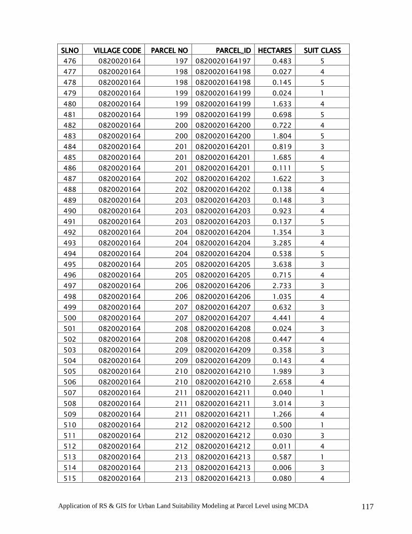
Application of RS & GIS for Urban Land Suitability Modeling at Parcel Level using MCDA 117
SLNOSLNOSLNOSLNO VILLAGEVILLAGEVILLAGEVILLAGE CODECODECODECODE PARCELPARCELPARCELPARCEL NONONONO PARCEL_IDPARCEL_IDPARCEL_IDPARCEL_ID HECTARESHECTARESHECTARESHECTARES SUIT CLASSSUIT CLASSSUIT CLASSSUIT CLASS
476 0820020164 197 0820020164197 0.483 5
477 0820020164 198 0820020164198 0.027 4
478 0820020164 198 0820020164198 0.145 5
479 0820020164 199 0820020164199 0.024 1
480 0820020164 199 0820020164199 1.633 4
481 0820020164 199 0820020164199 0.698 5
482 0820020164 200 0820020164200 0.722 4
483 0820020164 200 0820020164200 1.804 5
484 0820020164 201 0820020164201 0.819 3
485 0820020164 201 0820020164201 1.685 4
486 0820020164 201 0820020164201 0.111 5
487 0820020164 202 0820020164202 1.622 3
488 0820020164 202 0820020164202 0.138 4
489 0820020164 203 0820020164203 0.148 3
490 0820020164 203 0820020164203 0.923 4
491 0820020164 203 0820020164203 0.137 5
492 0820020164 204 0820020164204 1.354 3
493 0820020164 204 0820020164204 3.285 4
494 0820020164 204 0820020164204 0.538 5
495 0820020164 205 0820020164205 3.638 3
496 0820020164 205 0820020164205 0.715 4
497 0820020164 206 0820020164206 2.733 3
498 0820020164 206 0820020164206 1.035 4
499 0820020164 207 0820020164207 0.632 3
500 0820020164 207 0820020164207 4.441 4
501 0820020164 208 0820020164208 0.024 3
502 0820020164 208 0820020164208 0.447 4
503 0820020164 209 0820020164209 0.358 3
504 0820020164 209 0820020164209 0.143 4
505 0820020164 210 0820020164210 1.989 3
506 0820020164 210 0820020164210 2.658 4
507 0820020164 211 0820020164211 0.040 1
508 0820020164 211 0820020164211 3.014 3
509 0820020164 211 0820020164211 1.266 4
510 0820020164 212 0820020164212 0.500 1
511 0820020164 212 0820020164212 0.030 3
512 0820020164 212 0820020164212 0.011 4
513 0820020164 213 0820020164213 0.587 1
514 0820020164 213 0820020164213 0.006 3
515 0820020164 213 0820020164213 0.080 4

Application of RS & GIS for Urban Land Suitability Modeling at Parcel Level using MCDA 118
SLNOSLNOSLNOSLNO VILLAGEVILLAGEVILLAGEVILLAGE CODECODECODECODE PARCELPARCELPARCELPARCEL NONONONO PARCEL_IDPARCEL_IDPARCEL_IDPARCEL_ID HECTARESHECTARESHECTARESHECTARES SUIT CLASSSUIT CLASSSUIT CLASSSUIT CLASS
516 0820020164 214 0820020164214 0.636 1
517 0820020164 214 0820020164214 0.826 3
518 0820020164 214 0820020164214 0.841 4
519 0820020164 215 0820020164215 5.015 1
520 0820020164 215 0820020164215 0.055 3
521 0820020164 215 0820020164215 0.076 4
522 0820020164 217 0820020164217 1.678 1
523 0820020164 217 0820020164217 0.243 3
524 0820020164 217 0820020164217 1.148 4
525 0820020164 218 0820020164218 0.676 1
526 0820020164 219 0820020164219 3.363 1
527 0820020164 219 0820020164219 0.427 3
528 0820020164 219 0820020164219 0.422 4
529 0820020164 220 0820020164220 3.647 3
530 0820020164 220 0820020164220 1.600 4
531 0820020164 221 0820020164221 0.016 3
532 0820020164 221 0820020164221 1.063 4
533 0820020164 222 0820020164222 0.502 3
534 0820020164 222 0820020164222 1.296 4
535 0820020164 223 0820020164223 0.254 4
536 0820020164 224 0820020164224 1.892 1
537 0820020164 224 0820020164224 1.109 3
538 0820020164 224 0820020164224 0.324 4
539 0820020164 225 0820020164225 0.448 1
540 0820020164 225 0820020164225 0.533 3
541 0820020164 225 0820020164225 0.003 4
542 0820020164 226 0820020164226 0.777 1
543 0820020164 226 0820020164226 0.019 3
544 0820020164 226 0820020164226 0.256 4
545 0820020164 227 0820020164227 1.835 1
546 0820020164 227 0820020164227 0.692 3
547 0820020164 227 0820020164227 0.615 4
548 0820020164 228 0820020164228 0.903 1
549 0820020164 228 0820020164228 2.711 3
550 0820020164 228 0820020164228 0.060 4
551 0820020164 229 0820020164229 6.201 3
552 0820020164 229 0820020164229 0.035 4
553 0820020164 230 0820020164230 2.265 3
554 0820020164 230 0820020164230 2.127 4
555 0820020164 231 0820020164231 1.115 3

Application of RS & GIS for Urban Land Suitability Modeling at Parcel Level using MCDA 119
SLNOSLNOSLNOSLNO VILLAGEVILLAGEVILLAGEVILLAGE CODECODECODECODE PARCELPARCELPARCELPARCEL NONONONO PARCEL_IDPARCEL_IDPARCEL_IDPARCEL_ID HECTARESHECTARESHECTARESHECTARES SUIT CLASSSUIT CLASSSUIT CLASSSUIT CLASS
556 0820020164 231 0820020164231 0.664 4
557 0820020164 232 0820020164232 1.752 3
558 0820020164 232 0820020164232 2.696 4
559 0820020164 233 0820020164233 0.210 1
560 0820020164 233 0820020164233 1.246 3
561 0820020164 233 0820020164233 0.006 4
562 0820020164 234 0820020164234 4.353 3
563 0820020164 234 0820020164234 0.020 4
564 0820020164 235 0820020164235 2.564 1
565 0820020164 235 0820020164235 0.114 3
566 0820020164 236 0820020164236 0.085 1
567 0820020164 236 0820020164236 0.960 3
568 0820020164 236 0820020164236 0.494 4
569 0820020164 237 0820020164237 1.550 1
570 0820020164 237 0820020164237 0.034 3
571 0820020164 241 0820020164241 1.222 1
572 0820020164 242 0820020164242 0.231 1
573 0820020164 243 0820020164243 3.085 1
574 0820020164 244 0820020164244 0.323 1
575 0820020164 245 0820020164245 3.496 1
576 0820020164 246 0820020164246 0.844 1
577 0820020164 246 0820020164246 0.426 3
578 0820020164 247 0820020164247 1.077 3
579 0820020164 248 0820020164248 0.604 1
580 0820020164 248 0820020164248 0.541 3
581 0820020164 249 0820020164249 0.670 1
582 0820020164 249 0820020164249 1.296 3
583 0820020164 250 0820020164250 0.178 3
584 0820020164 251 0820020164251 0.393 1
585 0820020164 251 0820020164251 0.790 3
586 0820020164 252 0820020164252 0.983 1
587 0820020164 252 0820020164252 0.000 3
588 0820020164 253 0820020164253 1.085 1
589 0820020164 253 0820020164253 0.139 3
590 0820020164 254 0820020164254 0.738 1
591 0820020164 254 0820020164254 0.656 3
592 0820020164 256 0820020164256 1.000 3
593 0820020164 256 0820020164256 0.015 4
594 0820020164 257 0820020164257 1.327 3
595 0820020164 257 0820020164257 0.212 4

Application of RS & GIS for Urban Land Suitability Modeling at Parcel Level using MCDA 120
SLNOSLNOSLNOSLNO VILLAGEVILLAGEVILLAGEVILLAGE CODECODECODECODE PARCEPARCEPARCEPARCELLLL NONONONO PARCEL_IDPARCEL_IDPARCEL_IDPARCEL_ID HECTARESHECTARESHECTARESHECTARES SUIT CLASSSUIT CLASSSUIT CLASSSUIT CLASS
596 0820020164 258 0820020164258 0.347 1
597 0820020164 258 0820020164258 0.946 3
598 0820020164 259 0820020164259 0.255 1
599 0820020164 259 0820020164259 0.878 3
600 0820020164 260 0820020164260 0.054 1
601 0820020164 260 0820020164260 0.293 3
602 0820020164 261 0820020164261 0.089 1
603 0820020164 261 0820020164261 0.106 1
604 0820020164 261 0820020164261 0.228 3
605 0820020164 262 0820020164262 0.007 1
606 0820020164 262 0820020164262 0.274 3
607 0820020164 262 0820020164262 0.003 4
608 0820020164 264 0820020164264 0.013 1
609 0820020164 264 0820020164264 0.640 4
610 0820020164 265 0820020164265 0.982 3
611 0820020164 265 0820020164265 0.813 4
612 0820020164 266 0820020164266 0.688 3
613 0820020164 266 0820020164266 2.748 4
614 0820020164 267 0820020164267 2.575 3
615 0820020164 267 0820020164267 1.460 4
616 0820020164 268 0820020164268 0.663 3
617 0820020164 268 0820020164268 3.021 4
618 0820020164 269 0820020164269 4.233 3
619 0820020164 269 0820020164269 0.466 4
620 0820020164 270 0820020164270 4.597 3
621 0820020164 270 0820020164270 1.318 4
622 0820020164 271 0820020164271 5.359 3
623 0820020164 271 0820020164271 0.019 4
624 0820020164 272 0820020164272 3.913 3
625 0820020164 272 0820020164272 0.376 4
626 0820020164 273 0820020164273 2.103 3
627 0820020164 273 0820020164273 0.004 4
628 0820020164 274 0820020164274 2.373 3
629 0820020164 274 0820020164274 0.039 4
630 0820020164 275 0820020164275 3.815 3
631 0820020164 275 0820020164275 0.002 4
632 0820020164 276 0820020164276 0.001 1
633 0820020164 276 0820020164276 2.192 3
634 0820020164 276 0820020164276 1.739 4
635 0820020164 276 0820020164276 0.149 5

Application of RS & GIS for Urban Land Suitability Modeling at Parcel Level using MCDA 121
SLNOSLNOSLNOSLNO VILLAGEVILLAGEVILLAGEVILLAGE CODECODECODECODE PARCELPARCELPARCELPARCEL NONONONO PARCEL_IDPARCEL_IDPARCEL_IDPARCEL_ID HECTARESHECTARESHECTARESHECTARES SUIT CLASSSUIT CLASSSUIT CLASSSUIT CLASS
636 0820020164 277 0820020164277 0.895 3
637 0820020164 277 0820020164277 2.098 4
638 0820020164 277 0820020164277 0.909 5
639 0820020164 278 0820020164278 1.807 3
640 0820020164 278 0820020164278 0.016 4
641 0820020164 279 0820020164279 1.101 3
642 0820020164 279 0820020164279 2.919 4
643 0820020164 279 0820020164279 0.016 5
644 0820020164 280 0820020164280 0.693 3
645 0820020164 280 0820020164280 2.531 4
646 0820020164 280 0820020164280 0.434 5
647 0820020164 281 0820020164281 2.771 3
648 0820020164 281 0820020164281 2.354 4
649 0820020164 281 0820020164281 0.095 5
650 0820020164 282 0820020164282 0.915 3
651 0820020164 282 0820020164282 2.031 4
652 0820020164 283 0820020164283 1.063 3
653 0820020164 283 0820020164283 0.637 4
654 0820020164 284 0820020164284 3.406 3
655 0820020164 284 0820020164284 0.892 4
656 0820020164 285 0820020164285 0.588 3
657 0820020164 285 0820020164285 2.094 4
658 0820020164 286 0820020164286 0.136 3
659 0820020164 286 0820020164286 0.229 4
660 0820020164 287 0820020164287 1.830 3
661 0820020164 287 0820020164287 1.330 4
662 0820020164 288 0820020164288 0.681 3
663 0820020164 288 0820020164288 1.093 4
664 0820020164 289 0820020164289 0.439 1
665 0820020164 289 0820020164289 0.488 3
666 0820020164 289 0820020164289 3.503 4
667 0820020164 290 0820020164290 0.474 1
668 0820020164 290 0820020164290 0.019 4
669 0820020164 291 0820020164291 0.099 1
670 0820020164 291 0820020164291 0.000 3
671 0820020164 292 0820020164292 0.077 1
672 0820020164 292 0820020164292 1.261 3
673 0820020164 293 0820020164293 0.305 1
674 0820020164 293 0820020164293 0.022 2
675 0820020164 293 0820020164293 4.560 3

Application of RS & GIS for Urban Land Suitability Modeling at Parcel Level using MCDA 122
SLNOSLNOSLNOSLNO VILLAGEVILLAGEVILLAGEVILLAGE CODECODECODECODE PARCELPARCELPARCELPARCEL NONONONO PARCEL_IDPARCEL_IDPARCEL_IDPARCEL_ID HECTARESHECTARESHECTARESHECTARES SUIT CLASSSUIT CLASSSUIT CLASSSUIT CLASS
676 0820020164 293 0820020164293 0.258 4
677 0820020164 294 0820020164294 0.040 1
678 0820020164 294 0820020164294 0.214 2
679 0820020164 294 0820020164294 0.512 3
680 0820020164 294 0820020164294 0.654 4
681 0820020164 294 0820020164294 1.305 5
682 0820020164 295 0820020164295 0.132 1
683 0820020164 295 0820020164295 0.761 2
684 0820020164 295 0820020164295 1.283 4
685 0820020164 295 0820020164295 0.038 5
686 0820020164 296 0820020164296 0.015 1
687 0820020164 296 0820020164296 0.511 2
688 0820020164 296 0820020164296 0.049 3
689 0820020164 296 0820020164296 1.654 4
690 0820020164 296 0820020164296 0.695 5
691 0820020164 297 0820020164297 0.390 4
692 0820020164 297 0820020164297 1.208 5
693 0820020164 298 0820020164298 0.944 5
694 0820020164 299 0820020164299 0.173 4
695 0820020164 299 0820020164299 1.622 5
696 0820020164 300 0820020164300 0.797 2
697 0820020164 300 0820020164300 0.063 3
698 0820020164 300 0820020164300 1.039 4
699 0820020164 300 0820020164300 0.117 5
700 0820020164 301 0820020164301 24.230 1
701 0820020164 301 0820020164301 0.275 2
702 0820020164 301 0820020164301 0.589 3
703 0820020164 301 0820020164301 0.000 4
704 0820020164 302 0820020164302 4.602 1
705 0820020164 302 0820020164302 0.455 5
706 0820020164 303 0820020164303 0.006 1
707 0820020164 303 0820020164303 2.010 5
708 0820020164 304 0820020164304 2.814 1
709 0820020164 304 0820020164304 0.989 4
710 0820020164 305 0820020164305 1.036 1
711 0820020164 305 0820020164305 0.275 4
712 0820020164 306 0820020164306 2.277 1
713 0820020164 306 0820020164306 0.342 3
714 0820020164 306 0820020164306 0.116 4
715 0820020164 307 0820020164307 0.175 1

Application of RS & GIS for Urban Land Suitability Modeling at Parcel Level using MCDA 123
SLNOSLNOSLNOSLNO VILLAGEVILLAGEVILLAGEVILLAGE CODECODECODECODE PARCELPARCELPARCELPARCEL NONONONO PARCEL_IDPARCEL_IDPARCEL_IDPARCEL_ID HECTARESHECTARESHECTARESHECTARES SUIT CLASSSUIT CLASSSUIT CLASSSUIT CLASS
716 0820020164 308 0820020164308 0.258 1
717 0820020164 308 0820020164308 0.849 5
718 0820020164 309 0820020164309 0.216 1
719 0820020164 309 0820020164309 2.093 4
720 0820020164 309 0820020164309 0.143 5
721 0820020164 310 0820020164310 0.946 1
722 0820020164 310 0820020164310 1.149 5
723 0820020164 310 0820020164310 1.455 5
724 0820020164 312 0820020164312 2.077 1
725 0820020164 312 0820020164312 0.064 4
726 0820020164 312 0820020164312 0.398 5

Application of RS & GIS for Urban Land Suitability Modeling at Parcel Level using MCDA 124
References:References:References:References:
• BDA Master Plan - 2021 (Draft): 2005 : Published by Bangalore
Development Authority
• Burrogh P A and Mc Donneu R: Principles of Geographical Information
System, Oxford University Press, London
• Campbell Jhon, B: 1996 : Introduction to Remote Sensing, Taylor &
Francis.
• Census: 2001 : Bangalore Urban and Rural Districts
• ERDAS IMAGINE field guide
• ERDAS IMAGINE tour guide
• FAO: (1976) : A framework for land evaluation. Soil Bulletin 32, Food and
Agricultural Organization of United Nations, Rome
• Indore Development Plan 2011 (Draft) : 2003 : published by Directorate
of Town and Country Planning and ISRO, Ahmedabad
• Jacek Malczewski : 1999 : GIS and Multi-Criteria Decision Analysis, Jhon
Wiley & Sons
• James Heitzman: 2004: Network City Planning the Information Society in
Bangalore : Published by Oxford University Press, New Delhi
• Jenson Jhon ,R: 1996: Introcution to Digital Image Processing: A Remote
Sensing Perspective, II Edition, Prentice Hall
• Karnataka State Gazetteer: Bangalore District, 1990; Government of
Karnataka Publication
• K. S. Gopalan, Director, SAC, ISRO, Ahmedabad: High resolution imagery
for developmental planning with special reference to developing
economies
• Lillisand Thomas, M & Keifer, Ralph : 1993 : Remote Sensing Image
Interpretation, Third Edition, John Wiley
• Paul A Longley : 2001 : Geographic Information Systems and Science,
Jhon Wiley & Sons
‘A Land Use And Land Cover Classification System For Use With
Remote Sensor Data’ By James R. Anderson, Ernest E. Hardy, Jhon T.
Roach, and Richard E. Witmer

Application of RS & GIS for Urban Land Suitability Modeling at Parcel Level using MCDA 125
• Revised Development Plan of Ahmedabad 2011; Vol.1:Remote Sensing
and GIS Approach: Published by Ahmedabad Urban Development
Authority and ISRO, Ahmedabad.
• Soil Survey Manual : 1971 : Published by All India Soil and Landuse Survey
Organization, IARI, New Delhi
• Understanding GIS: the ARC/INFO Method
• Urban Developments Plan Formulation and Implementation (UDPFI)
Guidelines: 1996 : published by Ministry of Urban affairs and
Employment, Govt. of India.
• Using ArcVIEW: Tutorials
Internet Internet Internet Internet ReReReResources:sources:sources:sources:
• http://www.censusindia.net
• http://www.gisdevelopment.com
• http://www.kar.nic.in
• http://www.bangaloreit.com
• http://www.bdabangalore.org
• http://www.fao.org
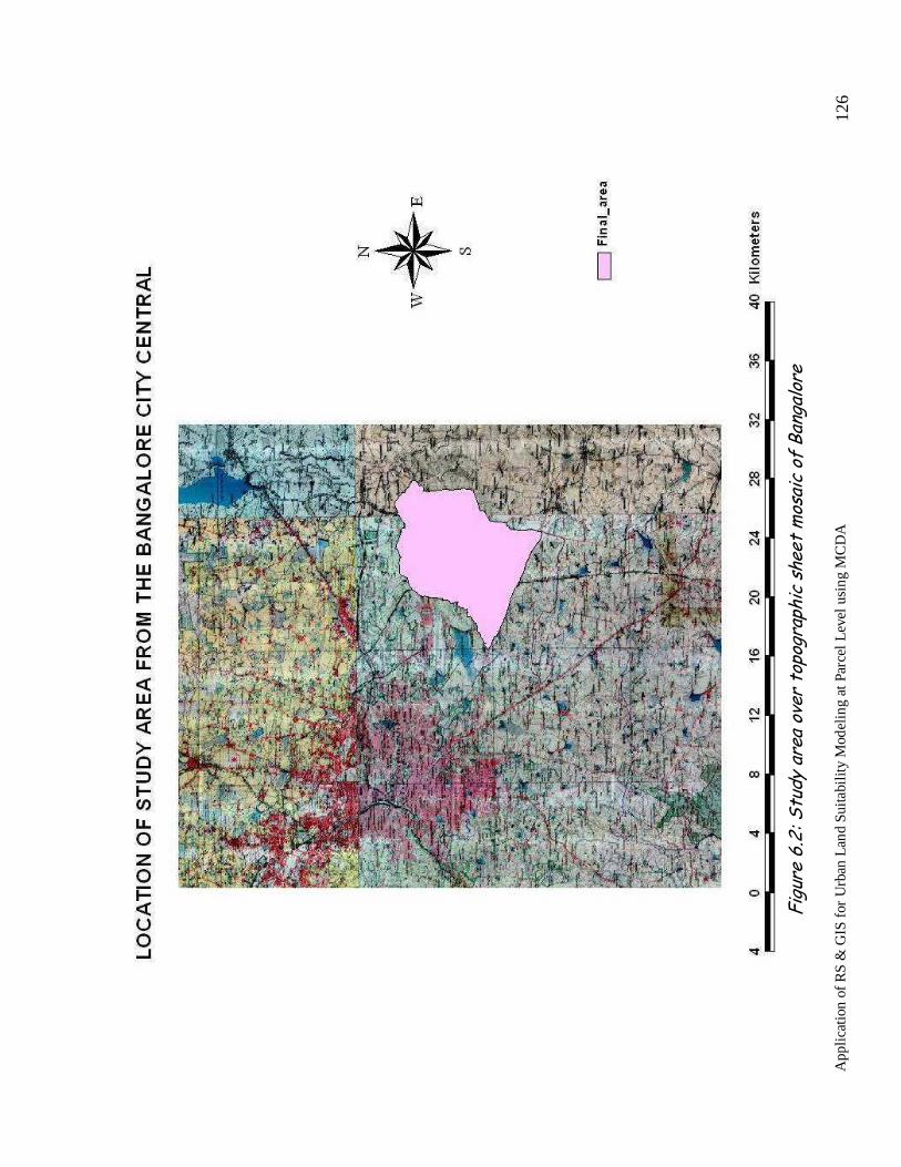
App
lica
tion
of
RS
& G
IS f
or U
rban
Lan
d Su
itabi
lity
Mod
elin
g at
Par
cel L
evel
usi
ng M
CD
A
126
Figur
e 6.3: Gro
wth
o B
anga
lore
city fr
om 1537 to 2001 (cen
sus 2001)
Figur
e 6.2: Stu
dy ar
ea ove
r to
pogr
aphic she
et m
osaic of
Ban
galore

App
lica
tion
of
RS
& G
IS f
or U
rban
Lan
d Su
itabi
lity
Mod
elin
g at
Par
cel L
evel
usi
ng M
CD
A
127
Figur
e 6.3: Lo
cation
of Stu
dy ar
ea ove
r M
aste
r Plan
( B
DA)

App
lica
tion
of
RS
& G
IS f
or U
rban
Lan
d Su
itabi
lity
Mod
elin
g at
Par
cel L
evel
usi
ng M
CD
A
128
Figur
e 6.4: Lo
cation
of st
udy ar
ea ove
r BDA A
dministr
ative Are
a

App
lica
tion
of
RS
& G
IS f
or U
rban
Lan
d Su
itabi
lity
Mod
elin
g at
Par
cel L
evel
usi
ng M
CD
A
129
Figur
e 7.2: Sub
set Stu
dy Are
a of
Quick
Bird M
erge
d Imag
e

App
lica
tion
of
RS
& G
IS f
or U
rban
Lan
d Su
itabi
lity
Mod
elin
g at
Par
cel L
evel
usi
ng M
CD
A
130
Figur
e 7.3: Existing
Man
ually
Digitized
Lan
duse
/lan
dco
ver M
ap

App
lica
tion
of
RS
& G
IS f
or U
rban
Lan
d Su
itabi
lity
Mod
elin
g at
Par
cel L
evel
usi
ng M
CD
A
131
Figur
e 7.4: Gro
und W
ater
Pro
spec
ts M
ap

App
lica
tion
of
RS
& G
IS f
or U
rban
Lan
d Su
itabi
lity
Mod
elin
g at
Par
cel L
evel
usi
ng M
CD
A
132
Figur
e 7.5: Soil Dep
th M
ap

App
lica
tion
of
RS
& G
IS f
or U
rban
Lan
d Su
itabi
lity
Mod
elin
g at
Par
cel L
evel
usi
ng M
CD
A
133
Figur
e 7.6: Soil Tex
ture
Map

App
lica
tion
of
RS
& G
IS f
or U
rban
Lan
d Su
itabi
lity
Mod
elin
g at
Par
cel L
evel
usi
ng M
CD
A
134
Figur
e 7.7: La
nd V
alue
(Gov
ernm
ent) M
ap

App
lica
tion
of
RS
& G
IS f
or U
rban
Lan
d Su
itabi
lity
Mod
elin
g at
Par
cel L
evel
usi
ng M
CD
A
135
Figur
e 7.9: Pr
oxim
ity to
Built-u
p Are
a M
ap

App
lica
tion
of
RS
& G
IS f
or U
rban
Lan
d Su
itabi
lity
Mod
elin
g at
Par
cel L
evel
usi
ng M
CD
A
136
Figur
e 7.8: Pr
oxim
ity to
Roa
d N
etwor
k Map

App
lica
tion
of
RS
& G
IS f
or U
rban
Lan
d Su
itabi
lity
Mod
elin
g at
Par
cel L
evel
usi
ng M
CD
A
137
Figur
e 7.10: M
aste
r Plan
Con
stra
int M
ap

App
lica
tion
of
RS
& G
IS f
or U
rban
Lan
d Su
itabi
lity
Mod
elin
g at
Par
cel L
evel
usi
ng M
CD
A
138
Figur
e 7.11: B
uilt-u
p Are
a Con
stra
int Map

App
lica
tion
of
RS
& G
IS f
or U
rban
Lan
d Su
itabi
lity
Mod
elin
g at
Par
cel L
evel
usi
ng M
CD
A
139
Figur
e 7.12: W
ater
Bod
ies Con
stra
int M
ap

App
lica
tion
of
RS
& G
IS f
or U
rban
Lan
d Su
itabi
lity
Mod
elin
g at
Par
cel L
evel
usi
ng M
CD
A
140
Figur
e 7.14: Ove
rlay
of Geo
-ref
eren
ced C
adas
tral M
ap of Gun
jur Villag
e ov
er Q
uick
Bird M
erge
d Imag
e

App
lica
tion
of
RS
& G
IS f
or U
rban
Lan
d Su
itabi
lity
Mod
elin
g at
Par
cel L
evel
usi
ng M
CD
A
141
Figur
e 7.16: Ove
rlay
of Cad
astr
al V
ecto
r Pa
rcel La
yer ov
er Q
uick
Bird Imag
e

App
lica
tion
of
RS
& G
IS f
or U
rban
Lan
d Su
itabi
lity
Mod
elin
g at
Par
cel L
evel
usi
ng M
CD
A
142
Figure 7.15: Village wise Parcel Vector Layer

App
lica
tion
of
RS
& G
IS f
or U
rban
Lan
d Su
itabi
lity
Mod
elin
g at
Par
cel L
evel
usi
ng M
CD
A
143
Figure 8.6 : Urban land Suitability Map For Urban Suitability Model 1

App
lica
tion
of
RS
& G
IS f
or U
rban
Lan
d Su
itabi
lity
Mod
elin
g at
Par
cel L
evel
usi
ng M
CD
A
144
Figure 8.7 : Urban land Suitability Map For Urban Suitability Model 2

App
lica
tion
of
RS
& G
IS f
or U
rban
Lan
d Su
itabi
lity
Mod
elin
g at
Par
cel L
evel
usi
ng M
CD
A
145
Figure 8.8 : Urban land Suitability Map For Urban Suitability Model 3

App
lica
tion
of
RS
& G
IS f
or U
rban
Lan
d Su
itabi
lity
Mod
elin
g at
Par
cel L
evel
usi
ng M
CD
A
146
Figure 8.9 : Urban land Suitability Map For Urban Suitability Model 4

App
lica
tion
of
RS
& G
IS f
or U
rban
Lan
d Su
itabi
lity
Mod
elin
g at
Par
cel L
evel
usi
ng M
CD
A
147
Figure 8.10 : Parcel Level Urban Land Suitability Map for Model – 1

App
lica
tion
of
RS
& G
IS f
or U
rban
Lan
d Su
itabi
lity
Mod
elin
g at
Par
cel L
evel
usi
ng M
CD
A
148
Figure 8.11 : Parcel Level Urban Land Suitability Map for Model – 2
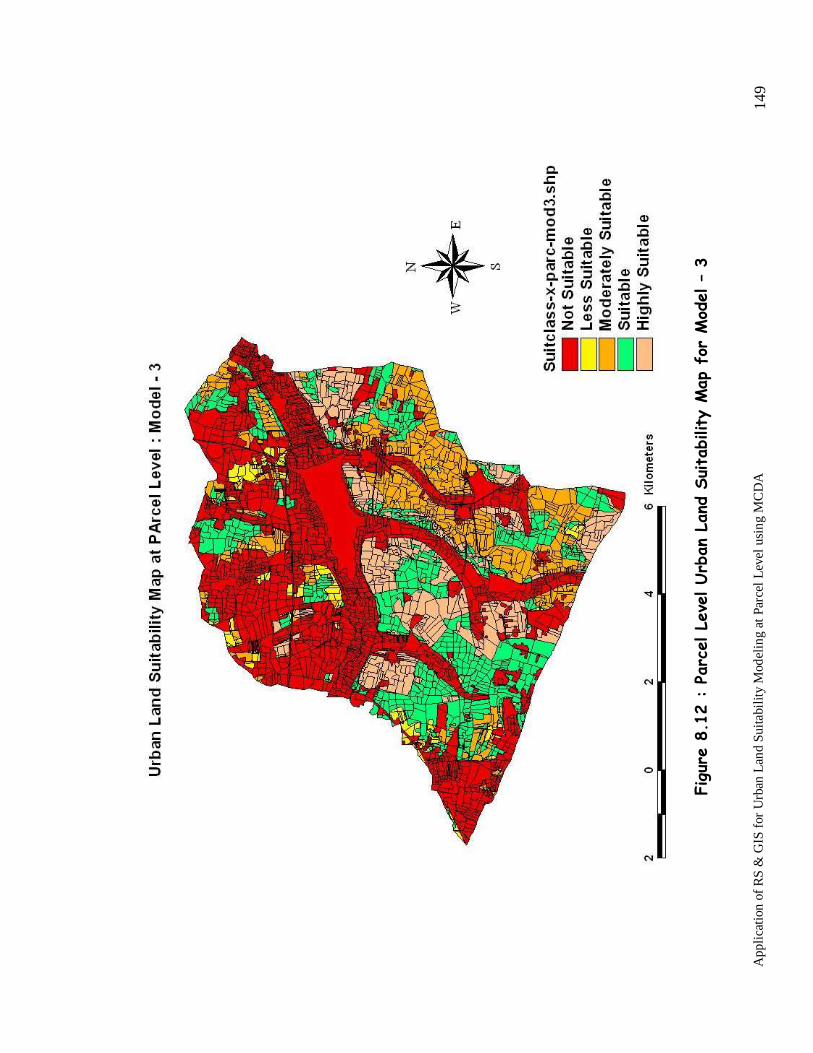
App
lica
tion
of
RS
& G
IS f
or U
rban
Lan
d Su
itabi
lity
Mod
elin
g at
Par
cel L
evel
usi
ng M
CD
A
149
Figure 8.12 : Parcel Level Urban Land Suitability Map for Model – 3

App
lica
tion
of
RS
& G
IS f
or U
rban
Lan
d Su
itabi
lity
Mod
elin
g at
Par
cel L
evel
usi
ng M
CD
A
150
Figure 8.13 : Parcel Level Urban Land Suitability Map for Model – 4
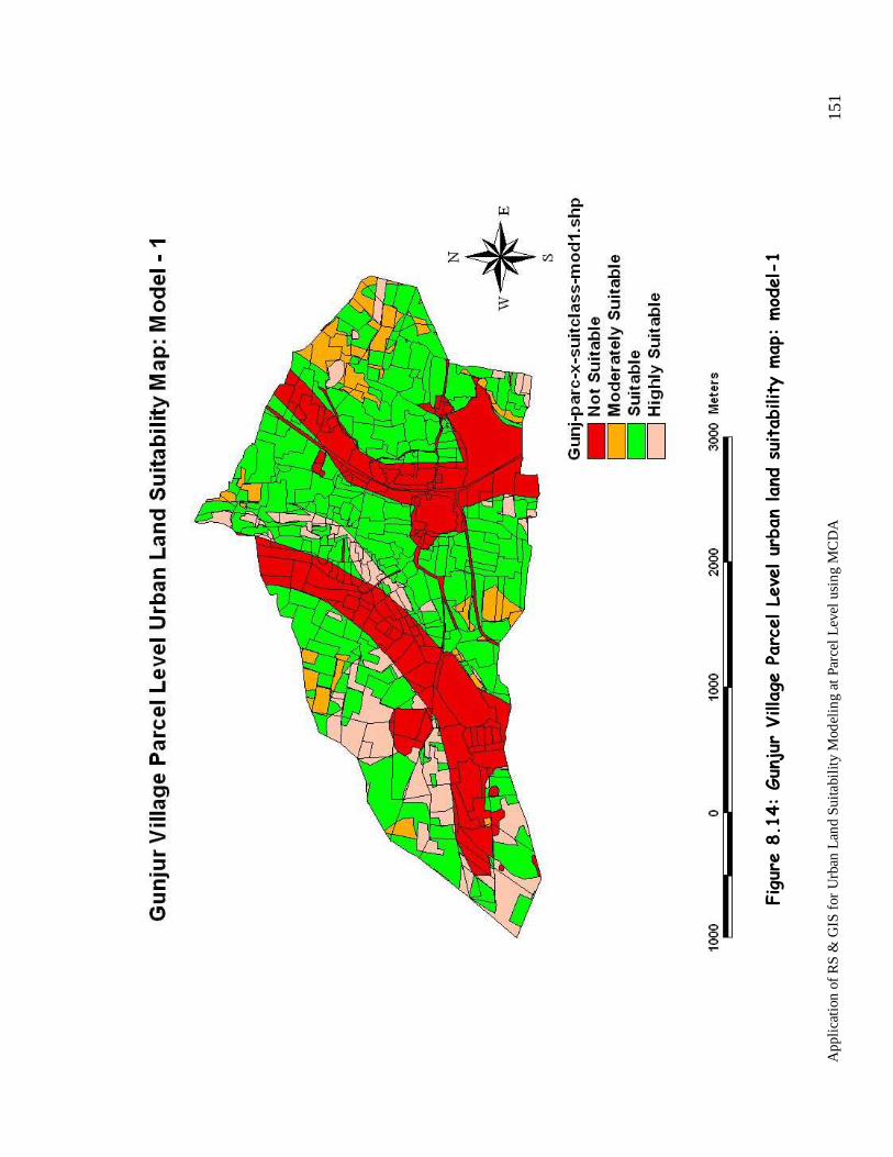
App
lica
tion
of
RS
& G
IS f
or U
rban
Lan
d Su
itabi
lity
Mod
elin
g at
Par
cel L
evel
usi
ng M
CD
A
151
Figure 8.14: Gunjur Village Parcel Level urban land suitability map: model-1

App
lica
tion
of
RS
& G
IS f
or U
rban
Lan
d Su
itabi
lity
Mod
elin
g at
Par
cel L
evel
usi
ng M
CD
A
152
Figure 8.15: Gunjur Village Parcel Level urban land suitability map: model-2

App
lica
tion
of
RS
& G
IS f
or U
rban
Lan
d Su
itabi
lity
Mod
elin
g at
Par
cel L
evel
usi
ng M
CD
A
153
Figure 8.16: Gunjur Village Parcel Level urban land suitability map: model-3

App
lica
tion
of
RS
& G
IS f
or U
rban
Lan
d Su
itabi
lity
Mod
elin
g at
Par
cel L
evel
usi
ng M
CD
A
154
Figure 8.17: Gunjur Village Parcel Level urban land suitability map: model-4

App
lica
tion
of
RS
& G
IS f
or U
rban
Lan
d Su
itabi
lity
Mod
elin
g at
Par
cel L
evel
usi
ng M
CD
A
155
Figure 8.18: Gunjur Village Parcel Level urban land suitability map for Parcel No: 303 : model-1

App
lica
tion
of
RS
& G
IS f
or U
rban
Lan
d Su
itabi
lity
Mod
elin
g at
Par
cel L
evel
usi
ng M
CD
A
156
Figure 8.19: Gunjur Village Parcel Level urban land suitability map for Parcel No: 303 : model-2

App
lica
tion
of
RS
& G
IS f
or U
rban
Lan
d Su
itabi
lity
Mod
elin
g at
Par
cel L
evel
usi
ng M
CD
A
157
Figure 8.20: Gunjur Village Parcel Level urban land suitability map for Parcel No: 303 : model-3
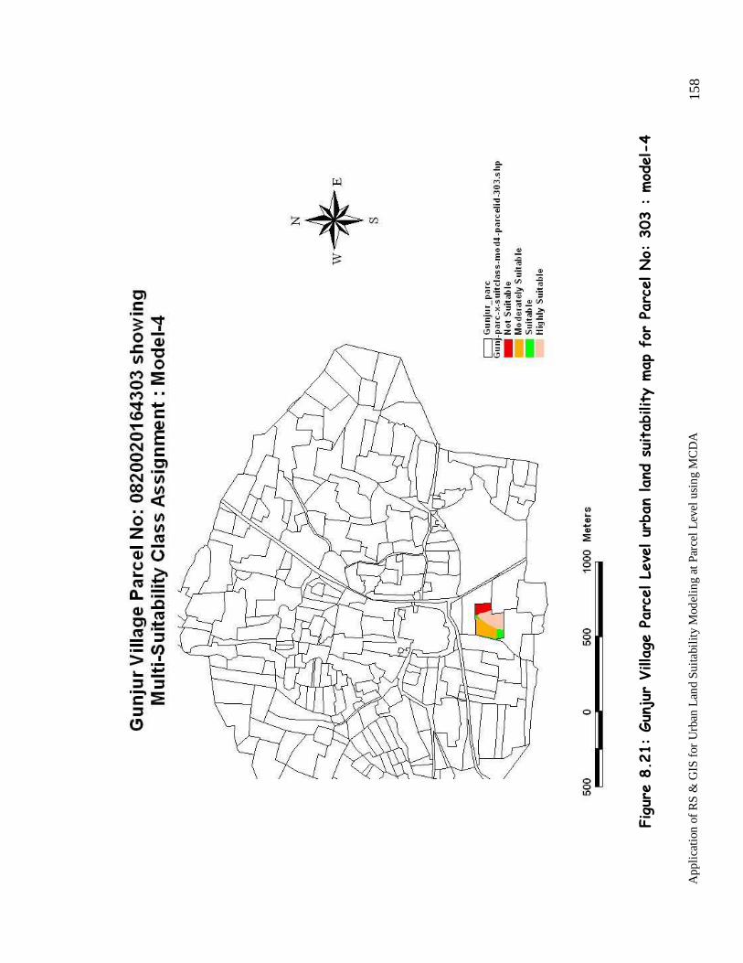
App
lica
tion
of
RS
& G
IS f
or U
rban
Lan
d Su
itabi
lity
Mod
elin
g at
Par
cel L
evel
usi
ng M
CD
A
158
Figure 8.21: Gunjur Village Parcel Level urban land suitability map for Parcel No: 303 : model-4