APPLICATION OF STATISTICALQUALITY CONTROL PROCEDURESTO PRODUCTION OF HIGHWAYPAVEMENT CONCRETE

Technical Paper

AFPLK^TION OF SIATISTICAL Q(Ua.ITY CONTROL PROCEDURES

TO PRODUCTION OP HIGHWAY PAVQIEHT CONCRETE

^°' ?•/: itT'"'^^^ ®^'^TL . . February 11, I966Joint Highway Research Project

File: 9-11-2From: H. L. Michael, Associate Director proiect: C-36-67B

Joint Highway Research Project

Attached Is a paper entitled "Application of StatisticalQuality Control Procedures to Production of Highway PavementConcrete" 'CO-auChored by S. J. Hanna, J. F. McLaughlin and A. P<

Lott.

This work was presented orally at the last meeting of theHighway Research Board. It is a sumn^ry of the first phase ofthe quality control project previously reported to the Board.Permission to publish this report in the HRB Research Record isrequested.

Respectfully submitted,

H. L. Michael, Secretary

Hm:kr

Attachment

cc: F. L. Ashbaucher F. B. MendenhallJ. R. Cooper R. D. MilesJ. W. Delleur J. C. OppenlanderW. L. Dolch W. P. PrlvetteW. H. Goet2 M. B. ScottW. L. Greece F. W. StubbsG. K. Hallock R. B. HoodsP. S. Hill E. J. YoderJ. F. McLaughlin

Technical Paper

APPLICATION OF STATISTICAL QUALITY CONTROL

PROCEDURES TO PRODUCTION OF HIGHWAY PAVEMENT CONCRETE

by

S. J. Hanna, Research AssistantJ. F. McLaughlin, Research EngineerA. P. Lott, Graduate Assistant

Joint Highway Research Project

Project: 0-36-6713

File: 9-11-2

Prepared as Part of an Investigation

Conducted by

Joint Highway Research ProjectEngineering Experiment Station

Purdue University

in cooperation with

Indiana State Highway Commission

and the

Bureau of Public RoadsU.S. Department of Commerce

Not Released for Publication

Subject to Change

Not Rev lewed ByIndiana State Highway Commlas ion

or the

Bureau of Public Roads

Purdue UniversityLafayette, Indiana

January I966

Digitized by the Internet Archive

in 2011 with funding from

LYRASIS members and Sloan Foundation; Indiana Department of Transportation

http://www.archive.org/details/applicationofstaOOhann

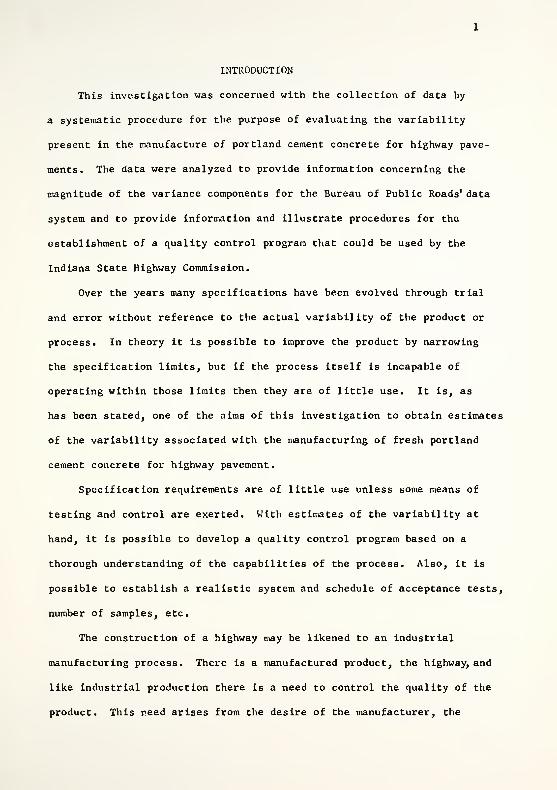
INTRODUCTION

This investigation was concerned with the collection of data by

a systematic procedure for the purpose of evaluating the variability

present in the manufacture of portland cement concrete for highway pave-

ments. The data were analyzed to provide information concerning the

magnitude of the variance components for the Bureau of Public Roads' data

system and to provide information and illustrate procedures for the

establishment of a quality control program that could be used by the

Indiana State Highway Commission.

Over the years many specifications have been evolved through trial

and error without reference to the actual variability of the product or

process. In theory it is possible to improve the product by narrowing

the specification limits, but if the process Itself is incapable of

operating within those limits then they are of little use. It is, as

has been stated, one of the aims of this Investigation to obtain estimates

of the variability associated with the manufacturing of fresh portland

cement concrete for highway pavement.

Specification requirements are of little use unless some means of

testing and control are exerted. With estimates of the variability at

hand, it is possible to develop a quality control program based on a

thorough understanding of the capabilities of the process. Also, it is

possible to establish a realistic system and schedule of acceptance tests,

number of samples, etc.

The construction of a highway may be likened to an industrial

manufacturing process. There is a manufactured product, the highway, and

like industrial production there is a need to control the quality of the

product. This need arises from the desire of the manufacturer, the

contractor, to produce a product for the purchaser, the State, in the

most economical manner possible while meeting the specifications for the

product. The purchaser in turn is interested in seeing that he obtains

a quality product.

Statistical quality control provides a means whereby a manufacturer

can derive maximum benefit from control testing of the manufactured

product. The basic concepts are applicable whether the product tie piston

rings or highway pavements. inherent in statistical analyses is the

ability to make estimates of population parameters from sample statistics

and to associate with these estimates of the probability of being in

error. Using statistical quality control procedures, a manufacturing

process can be investigated to detennine the range in values that one

can expect under existing conditions. This information is valuable to

the producer and to the purchaser. It can be used not only in determining

compliance with specifications but also to judge whether the construction

or manufacturing process is capable of producing the product within them.

If existing specifications are unrealistic with respect to an end result

or are economically unattainable, quality control data can provide a

basis for the development of revised standards.

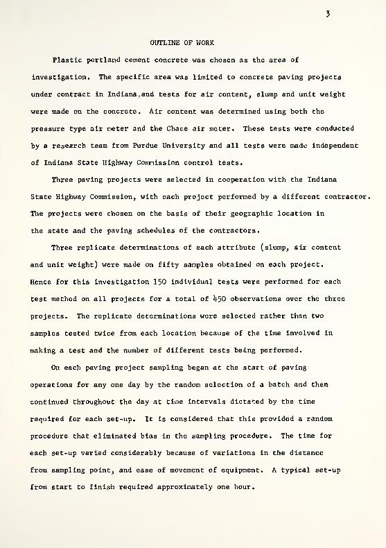
OUTLINE OF WORK

Plastic Portland cement concrete was chosen as the area of

investigation. The specific area was limited to concrete paving projects

under contract in Indiana. and tests for air content, slump and unit weight

were made on the concrete. Air content was determined using both the

pressure type air meter and the Chace air meter. These tests were conducted

by a research team from Purdue University and all tests were made independent

of Indiana State Highway Commission control tests.

Three paving projects were selected in cooperation with the Indiana

State Highway Commission, with each project performed by a different contractor.

The projects were chosen on the basis of their geographic location in

the state and the paving schedules of the contractors.

Three replicate determinations of each attribute (slump, air content

and unit weight) were made on fifty samples obtained on each project.

Hence for this investigation I50 individual tests were performed for each

test method on all projects for a total of k^O observations over the three

projects. The replicate determinations were selected rather than two

samples tested twice from each location because of the time Involved in

making a test and the number of different tests being performed.

On each paving project sampling began at the start of paving

operations for any one day by the random selection of a batch and then

continued throughout the day at time intervals dictated by the time

required for each set-up. It is considered that this provided a random

procedure that eliminated bias in the sampling procedure. The time for

each set-up varied considerably because of variations in the distance

from sampling point, and ease of movement of equipment. A typical set-up

from start to finish required approximately one hour.

The data were collected during the summer construction season of

l^k. The raw data were placed on IBM punch cards with appropriate coding

to indicate Job number, sample number, replicate number, time of test

and date test was made. The data were analyzed using standard statistical

techniques and procedures. The IBM 709'*- computer was utilized in the

data analysis.

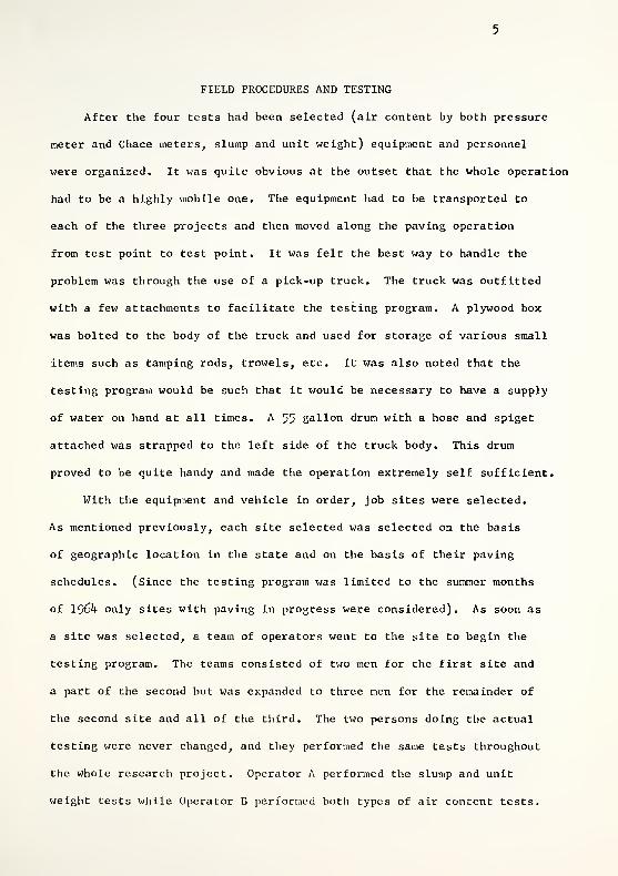
FIELD PROCEDURES AND TESTING

After the four tests had been selected (air content by both pressure

meter and Chace meters, slump and unit weight) equipment and personnel

were organized. It was quite obvious at the outset that the whole operation

had to be a highly mobile one. The equipment had to be transported to

each of the three projects and then moved along the paving operation

from test point to test point. It was felt the best way to handle the

problem was through the use of a pick-up truck. The truck was outfitted

with a few attachments to facilitate the testing program. A plywood box

was bolted to the body of the truck and used for storage of various small

items such as tamping rods, trowels, etc. It was also noted that the

testing program would be such that it would be necessary to have a supply

of water on hand at all times. A 55 gallon drum with a hose and spiget

attached was strapped to the left side of the truck body. This drum

proved to be quite handy and made the operation extremely self sufficient.

With the equipment and vehicle in order, job sites were selected.

As mentioned previously, each site selected was selected on the basis

of geographic location in the state and on the basis of their paving

schedules. (Since the testing program was limited to the summer months

of 196^ only sites with paving in progress were considered). As soon as

a site was selected, a team of operators went to the site to begin the

testing program. The teams consisted of two men for the first site and

a part of the second but was expanded to three men for the remainder of

the second site and all of the third. The tv^o persons doing the actual

testing were never changed, and they performed the same tests throughout

the whole research project. Operator A performed the slump and unit

weight tests while Operator B performed both types of air content tests.

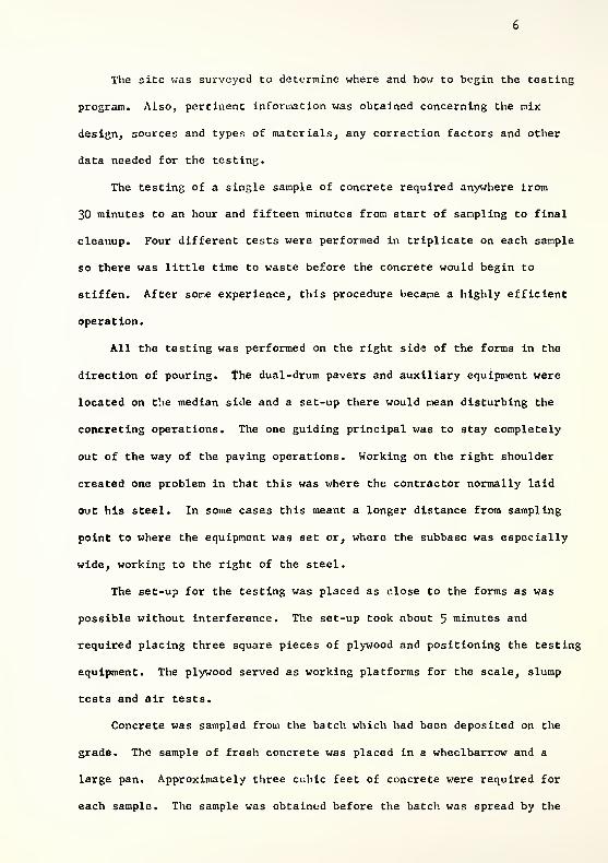
The site was surveyed to determine where and how to begin the testing

program. Also, pertinent information was obtained concerning the mix

design, sources and types of materials, any correction factors and other

data needed for the testing.

The testing of a single sample of concrete required anywhere from

30 minutes to an hour and fifteen minutes from start of sampling to final

cleanup. Four different tests were performed in triplicate on each sample

so there was little time to waste before the concrete would begin to

stiffen. After some experience, this procedure became a highly efficient

operation.

All the testing was performed on the right sids of the forms in the

direction of pouring, the dual-drum pavers and auxiliary equipment were

located on the median side and a set-up there would mean disturbing the

concreting operations. The one guiding principal was to stay completely

out of the way of the paving operations. Working on the right shoulder

created one problem in that this was where the contractor normally laid

out his steel. In some cases this meant a longer distance from sampling

point to where the equipment was set or, where the subbase was especially

wide, working to the right of the steel.

The set-up for the testing was placed as «:lose to the forms as was

possible without Interference. The set-up took about 5 minutes and

required placing three square pieces of plywood and positioning the testing

equipment. The plywood served as working platforms for the scale, slump

tests and air tests.

Concrete was sampled from the batch which had been deposited on the

grade. The sample of fresh concrete was placed in a wheelbarrow and a

large pan. Approximately three cubic feet of concrete were required for

each sample. The sample was obtained before the batch was spread by the

first spreader In tlie case of an operation using twin-barrel mixes and

after the Initial spread in the case of a central mix operation. The

distance between samples was quite arbitrary and depended upon how far

the paving train progressed between set-ups and how long it took the team

to perform the tests. The sampling operation required a maximum of 5

minutes.

With the concrete sample having been obtained, the tests themselves

were performed. Both Operators A and B started simultaneously performing

their respective tests. The equipment was positioned so the testing

could begin immediately to provide the maximum amount of time before the

concrete began to stiffen. Operator B immediately started perfoirming the

air content test by the pressure method while Operator A started on the

slump tests. These tests were performed in accordance with ASTM standards.

8

ANALYSIS OF DATA

At the completion of the testing program all data were tabulated

and recorded on IBM punch cards. Information regarding job number,

sample number, replicate number, time of test and date was coded and

placed on the punch cards along with the appropriate data for ease of

Identification. The statistical analysis of the data was accomplished

using standard computer programs for analysis of variance, correlation

and distribution. In addition, standard statistical techniques and

procedures were utilized to determine confidence limits, control limits

and in significance testing. A majority of the analyses and plotting

of data was accomplished using the IBM 709^-1^10 computer system.

The data collected from each of the four tests (air content by

pressure meter, air content by Chace meter, slump and unit weight) were

analyzed separately and the sum of squares, mean squares and standard

deviations computed for each test method. The first analysis was based

upon a 2-factor factorial design model with three replicate observations

for one factor (samples). In addition, correlation coefficients were

determined for all combinations of the above mentioned tests. Sample

means were used in the correlations and data plotting.

In the development of a quality control program it is necessary to

obtain data from a process which is "in control," that is, from a process

in which the variability is due to chance causes alone and not to

assignable causes. From observations in the field, such as noting obvious

errors in air-entraining agent content, water content, etc. it can be

said that at certain times a portion of the variability noted in the

present investigation was due to assignable errors. For this reason a

one-way analysis of variance was conducted for each site separately in

addition to the factorial analysis.

In certain of the analyses it was noted that the magnitude of the

variance components differed from site to site. Analyzing the data for

each site separately allows the computation of these variance components

and makes it possible to compare the magnitude of the components from

site to site. A factorial analysis averages the variances from the

three sites and hence if at one or two sites the process is out of control,

there is no estimate available for the variance of an in control process.

In fact the factorial analysis is invalid if the variances are not

homogeneous (i.e., variances are not statistically equal).

The factorial analyses have been included in this report for the

purpose of illustrating this type of statistical procedure. If other

variables such as operator or equipment were included in an investigation

the factorial design model could be used in the analysis of the data.

It should be noted that operators and testing equipment were not

considered as variables in this investigation. Only one operator and

one piece of testing equipment was used throughout the investigation for

each test method. This necessarily limits the interpretation of the data.

The values of standard deviations and confidence limits cannot be applied

directly to a project on which several operators and several pieces of

testing equipment are used.

As a sample was tested in the field for air content by the pressure

meter, a time dependency was observed. This led to testing the differences

between replicates and calculation of the correlation coefficient associated

with the third pressure replicate versus the sample mean of the Chace

tests. Results of this phase of the investigation will be discussed in

a later section.

The test results were also used to illustrate techniques and

procedures that may be employed in a quality control program. Control

10

limits are illustrated in the section on Quality Control.

For simplicity and ease in handling the large amount of data, a

discussion of each test method will be presented separately. Sections

concerning correlations and quality control applications follow. A

summary of a portion of the basic statistical results is presented in

the Appendix.

Field Observations

Dual-drum pavers were used on Sites 1 and 3 while a central mix

plant was in operation on Site 2. These were quite different sets of

conditions depending on the type of paving operation being employed. The

basic difference between the sites was the method of mixing with all

other operations being essentially the same.

Each method of paving had its own characteristics of control with

respect to frequency of adjustment. Quite often with the dual -drum

pavers the water valve was adjusted and readjusted to allow more or less

water into each batch. This yielded many batches that were alternately

wet or dry. This variability in water content per batch was due also to

the use of dry and wet batches of aggregate.

In the central mix project there were fewer adjustments. The plant

was started up and checked at the start of the project but then almost

complete reliance was placed on the automatic features of the plant. Thus,

there was less checking and less control of the concrete. The major

problem was control of air content. By the time a low air content was

noticed and a message relayed to the plant to make the necessary changes,

many concrete trucks were either dumping or already on their way to the

grade with their 8 cubic yards of concrete. There was a large lag- time

between catching a low air reading and effecting a correction. This was

an unfortunate characteristic of the operation.

11

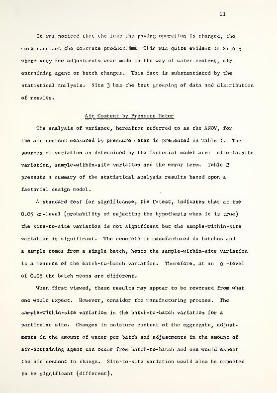
It was noticed that the less the paving operation is changed, the

more constant the concrete product. :§ This was quite evident at Site 3

v>7here very few adjustments were made in the way of water content, air

entraining agent or batch changes. This fact is substantiated by the

statistical analysis. Site 3 l^as the best grouping of data and distribution

of results.

Air Content by Pressure Meter

The analysis of variance, hereafter referred to as the ANOV, for

the air content measured by pressure meter is presented in Table 1. The

sources of variation as determined by the factorial model are: site-to-site

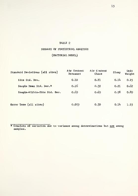
variation, sample-within-site variation and the error term. Table 2

presents a summary of the statistical analysis results based upon a

factorial design model.

A standard test for significance, the F-test, indicates that at the

0.05 a -level (probability of rejecting the hypothesis when it is true)

the site-to-site variation is not significant but the sample-within-site

variation is significant. The concrete is manufactured in batches and

a sample comes from a single batch, hence the sample-within-site variation

is a measure of the batch-to-batch variation. Therefore, at an a -level

of 0.05 the batch means are different.

When first viewed, these results may appear to be reversed from what

one would expect. However, consider the manufacturing process. The

sample-within-site variation is the batch-to-batch variation for a

particular site. Changes in moisture content of the aggregate, adjust-

ments in the amount of water per batch and adjustments in the amount of

air-entraining agent can occur from batch-to-batch and one would expect

the air content to change. Site-to-site variation would also be expected

to be significant (different).

^ Ont~ OOJ o>H

0)-p•H

CVJ Uo

^

12

CM UO

CM ta

CO

•a 1J

CM WD

8

00

CM

CM w CM W

Q CM

I ^

IfN ^

CO

CM

CM

CO

J-

1H

o o

4*

•51 «) ^^1

t4 +> d0) 4> « ^U «4 H W «H

II4) B* o H

1

1 Vo p•H •H

•H

«C•r

CO -P

+> •Si VO

aro

^ ^4)4* 1

^

II

00

II

CM

V &

ro

15

TABLE 2

SUMMARY OF STATISTICAL ANALYSES

(FACTORIAL MODEL)

Air ContentPressure

Air CmtentChace

SlumpUnit

Weight

0.10 0.11 O.lU 0.15

0.16 0.32 0.21 0.62

0.69 0.69 0.98 0.89

Standard Deviations (all sites)

Site Std. Dev.

Sample Mean Std. Dev.*

Sample-Within-Site Std. Dev.

Error Term (all sites) 0.079 O.3O O.II+ I.I5

* Consists of variation due to variance among determinations but not amongsamples.

Ik

It is neccGsary to understand the composition of the site-to-site

variance, or in statistical terms, the expected mean square (EMS)

2 2components of variance. The EMS from Table 1 is (a + 3cr , +

' e samplep op

150 a , ) for the yite to site component: (or'^ + 3^ i ) for the

^ site' e sample'2

sample-within-site component and a for the error term. The error term

(cr '^) is observed to be small in comparison to the sample-within-site

2 2term (a + 3^ ) leading to the conclusion that sample-within-site

2variation is significant or that sample means are different. The a

2term is large compared to the a , term and when a significance test is

? ? 2 2 2performed: (a + 3o + 150 a .^ )/ (cr + 3o ) the site-to-site

component is determined not significant. If the distribution of sample

2 2means was smaller (i.e. a smaller) and cr . remained the same, a

^ s ' site '

significance test might indicate the site-to-site component significant.

In other words distribution of sample means is so large that it over-

shadows the spread among site means.

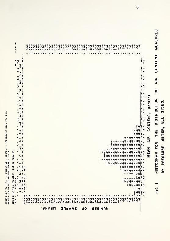
The distribution of air content for all sites measured by the pressure

meter is shown in Figure 1. Values tabulated are sample means. The over-

all mean air content is k,kO percent. The distribution over all sites

approximates a normal distribution. The air content determinations for

Sites 1 and 3 show some tendency towards normality but for Site 2 the

distribution was definitely not normal. This may be accounted for by

the fact that a number of difficulties arose with the plant operation on

Site 2. The aggregate varied considerably in its moisture content and

a number of failures occurred in the air entraining agent dispensing

equipment. These factors combined to produce a large range in air contents

and a non-normal distribution.

The observed error term from Table 2 is 0.079> or from a practical

viewpoint 0.1^, indicating that an error of 0.1^ can occur in the air

15

ooooooooooooooooooooooooooooooooooooooooooooooooooo^QOf^^u^<rK\^JlMO<^cDr^^u^^rr^(^l-^oC'X}^--ct/^^r'^^>J-^oc^(C^-•Oi^^<4'r1^(^l-dO(^<s^<Ol'^'#f'>'^•^

oliJ

DC3<UJ

UlHZoo

<

o

zo

3OQ

UJ

CO

a. <O Jo o

zIII

Zoo

DC

<

<111

"»-••-•<-< C <-• -^f

Q <

UJ OC

"- a:

2<DC<DOV)

tnUJa:Q.

>-m

a. a «t

_, 12 > o«I o n >

a z fSI

z — zo t/i

zO I O It

IT t- uo ^ zo < oc •<•

X Ui »x

lOOOOOOOOOOOOOOOOOOOOOOOOOOOOOOOOOOOOOOOOOOOOODOO

SNV3W 3"ldlNVS dO a39WnN

16

content determination due to chance alone. Placing 95^" confidence limits

on the site mean gives a range within which we are 95^ confident the true

site mean lies. For example, the mean for Site 1 is k.k&jo, therefore,

we are 95^0 confident that the true site mean lies between k.28ffi and U.68^.

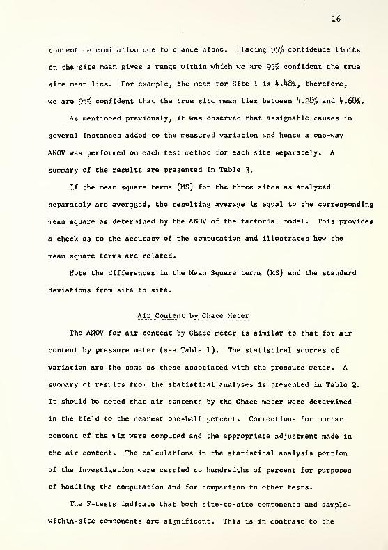
As mentioned previously, it was observed that assignable causes in

several instances added to the measured variation and hence a one-way

ANOV was performed on each test method for each site separately. A

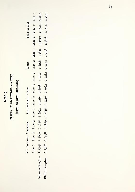
summary of the results are presented in Table 3«

If the mean square terms (MS) for the three sites as analyzed

separately are averaged, the resulting average is equal to the corresponding

mean square as determined by the ANOV of the factorial model. This provides

a check as to the accuracy of the computation and illustrates how the

mean square terms are related.

Note the differences in the Mean Square terms (MS) and the standard

deviations from site to site.

Air Content by Chace Meter

The ANOV for air content by Chace meter is similar to that for air

content by pressure meter (see Table l). The statistical sources of

variation are the same as those associated with the pressure meter. A

summary of results from the statistical analyses is presented in Table 2.

It should be noted that air contents by the Chace meter were determined

In the field to the nearest one-half percent. Corrections for mortar

content of the mix were computed and the appropriate adjustment made In

the air content. The calculations in the statistical analysis portion

of the investigation were carried to hundredths of percent for purposes

of handling the computation and for comparison to other tests.

The F-tests indicate that both site-to-site components and sample-

wlthln-site components are significant. This is in contrast to the

17

CO

CO

Z H

^

crt l-< r-VO co

0) CVJ J-4J ^ -*•WCO OJ 6u

4=<M ^

0) 0) VO -*s 4J VO CO

•r4 •

4J cn ^ i-H

f-l

c3 t-H ON -;t-* ro

V ON J--u .=^ VO1-1

CO OO I-l

CO^ O

0) 3" t-ij f-< o1-1 •

CO CO 6

CM CO COa. 8 COB 4) r-l

3 u 00 1-4

i-l •I-l •

M CO 1-1 o

I-l t-l CMON VO

<u r-1 CM4J O CM•MCO -^ 6

0)

CO

0) 1CM

U 4-1 VO 1-1

51-1

CO d aO

•\ OJ u^ VOu .-1 LPv

C 0) <M CO<u u O CM4J 1^4

gCO oJ 6

i-< CO l/N

>-l ON t-•H <u o 1^< 4J VO -^H • •

CO OJ o

CO VO C3N0) f-l 1-)

u 0) rM J-3 4J CO o(0 1-1 •

m CO o d0)

OJ ^ OOITS

•* ti VO ITNu u l/N oCi •r* •

<u CO CM duco 1-1 IfN t—o -^ CO

V CO COl4 4J r-H I-l1-1 1-< • •

<: CO 1-1 o

CO

B 5

18

previously discussed pressure meter results where the site-to-site

components were not significant. The standard deviations computed for

the Chace test are 0.11 percent for the site means and 0.32 percent for

the sample means. It may be noted that the standard deviation for the

Chace meter sample means is twice that of the pressure meter. Again it

is pointed out that air contents by Chace meter are determined to the

nearest one-half percent in the field and that the Chace test might well

be used as an indicator of the relative air content but not as a test to

determine the precise air content. The samplt;-wtthin-site standard

deviation is O.69 percent which is the same as the pressure meter.

A histogram showing the distribution of air content by the Chace

meter for all sites is presented in Figure 2. The values plotted are

sample means. This distribution does approach a normal distribution,

but an interesting observation may be made. The figure shows three

distinct small peaks. These peaks occur at the mean Chace air content

for each site or if one were to locate the means of each site on Figure 2,

they would fall at each peak. This does not happen in the case of

pressure meter results as Figure 1 clearly shows. The pressure meter

distribution is nearer to a normal distribution. The distribution for

Chace is more disperse, thus showing its higher variability as indicated

by the higher standard deviation calculated for sample means.

From Table 2 the site to site standard deviation is 0.3^. Confidence

limits placed on the site mean indicate that there is a confidence of 95/^

that the site mean lies between X ,^ + 0.2°;o and X . - O.P^j. Also, thesite ' site '

95^ confidence limits on a sample mean is X , 0.6'/3. This last'^'^' ' sample - '

figure is interesting when it is compared to the pressure meter results.

In the analysis of the pressure meter data 95'/^ confidence limits were

determined to be X _ O.S'Jb (Table 1). This, once again indicates

19

OOOOOOOOOOOCJOOOOOOOOOOOOOOOOOOOOOOOOOOOOOOOOOOOOOO

X no •

i !

zLU1-

Zoo

(C

c <»u

U-« oQ.

Kzo CO

UJ

Z 1- l-Ui n»- m to

7oo _J

o <q:

< UJUJ

— oo <

> -J- •

JOOOOOOOOOOOOOOOOOOOOOOOOOOOOOOOOOOOOOOOOOOOOiDOO|DOOD <Z UJ

k> tA ^ m f^ '^

< •^UJ q:

ou. UJ

o<

2 X< oOH<s> Vo m1-mX

CVJ

o

SNV3IM 3idwvs JO aaawoN

20

the pressure air content test to be statistically more reliable than the

Chace test.

If one were to compare the three sites in an effort to check dispersion

of data, Site 3 stands out as being more consistent than the other two

sites. This is true because there were few adjustments made in the air

entraining agent and also less changing of the water content. Site 2

shows a sort of "sinusoidal" shape indicating trends which were not

immediate but occurred over a number of samples. A plot of the pressure

air content data also substantiates this. Site 2 was a central mix

project and this operation had difficulties with its air dispenser which

resulted in the distribution indicated. Site 2 also has the greatest

amount of dispersion of the three sites.

As in the pressure meter analysis, a one-way ANOV was conducted, and

the results are summarized in Table 3« Again observable differences occur

in the MS and standard deviation terms from site to site. As in the

pressure method analysis, the within Sample Means Square term for Site 1

is at least twice that of Sites 2 and 3 which are very nearly equal.

Slump Test

The ANOV for the slump test is similar to that in Table 1. The

sources of variation (site-to-site variation, sample-within-site and error

terms) are the same used for the two air content tests. Table 2 gives a

summary of the statistical analysis of the slump phase of this investigation

for the factorial model.

The F-test indicates that at a 0.05 a -level the site-to-site

variation is not significant but the sample-within-site variation is.

This is what would be expected in light of the characteristics of the

slump test. The slump test is a measure of water content and therefore

21

will vary as the water content varies. The more one changes the adjust-

ment on the water indicator of a mixer the more the slump should change.

In the light of this, one would expect Site 2, the central mix project,

to show the least variation in slump which it does. Both the dual-drum

paver sites show more spread in slump than Site 2. In the central mix

operation there were relatively few changes in water content compared to

the operations using dual-drum pavers.

The distribution of slump for all sites is presented in Figure 3»

The values therein plotted are sample means. The histogram shows a close

grouping of data which is a tight, almost normal, distribution. The

overall mean of the slump is, for all practical purposes, three inches.

There is a slight tendency for each site to approximate a normal distribution

which becomer more pronobnced when all three sites are lumped in Figure 3»

The histogram for Site 2 is tighter than those for Sites 1 and 3 which

substantiates what was said above concerning the central mix plant.

The 95fo confidence limits on the site mean are t O.jfo while 95^

confidence limits on the sample mean are _ O.Vjb. Site 2 had the smallest

range in slump values, i.e., it exhibited both the highest minimum and

lo\i/est niaximum slump.

As in the previous analyses, a one-v;ay ANOV was performed on the

slump data for each site and a summary of these results are presented in

Table 3« Note that the between sample standard deviation is lowest for

Site 2 bearing out the observation made from the factorial analysis that

the variances for Site 2 were smaller, i.e. Site 2 exhibited better

control as far as slump measurements were concerned.

Unit Weight

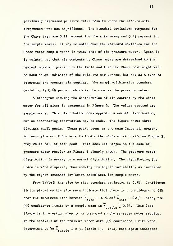
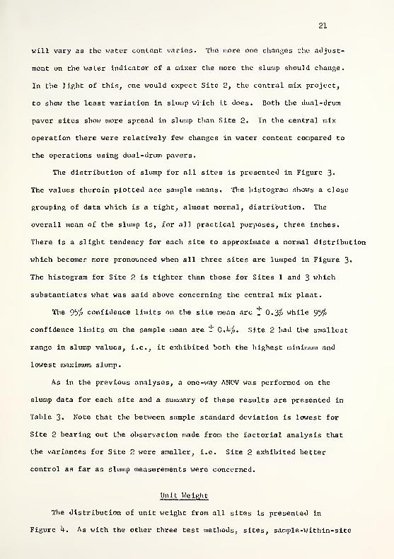
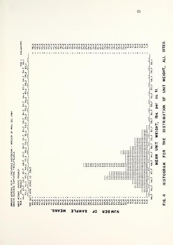
The distribution of unit weight from all sites is presented in

Figure h. As with the other three test methods, sites, sample-within-site

oooooooooocooooooooooooooooooooooooooooooooooooooo

UJ

Q.

ll.

o

zo

300

orz3-I

<2

o

<

ou.

I D

C 3

2<IT

o

< 'J

z —UJ O

o zir »-O -J

QC O -^> < I ^ -« ^ ^ •

X (—-#— +

(- I ^ -. ^ «.

-JOOOOOOOOOOOOOOOOOOOOOOOOOOOOOOOOOOOOOOOOOOOOOOOOOO

to

SNV31N 3ndk^VS dO d38kMnN

23

oooooooooooooooooooooooooooooooooooooooooooooooooo00'CDr-Ol/^^r'*l^sJ— oa'00^-^u^^fn(SlF^O(^»r<)lf^4•^*lN•-•O^0D^•-o^/^^p^<^J.-«O^{t>^-0^f>*^rg^

toUJ

to

CO t

• *

IT rg •

• +

^ *

XoUJ

z3

u.o

o.

a: < r- ir\ «.

O «ioo cr

*- Z) -i- r^

« >X t- nT +

o -» 00

z ^ 'T OJ« oo -rf 03 o3 U- *

o oo o lf\

7 7 -) •*

nex. -^

I 3 a. O-Q.

»- X. f^ ^CI o_J o c <a. ^ o o

-f o h- ^ + 1/1

+< o oa ^ 'T * z

* <z — X •-* ir\ I

z<UJ

2

o

mq:I-to

a

UJX

O

<o:CDoHto

ox X N ^

o <X lUa X

lOOOOOOOOOOOOOOOOOOOOOOOOOOOOOOOOOOOOOOOOOOOOOOOOOOrg^O0'«^-*0tr-#f*^(^t^O9'flDr^^DU^•r«^N•^off>00h->0ll^•#(nrg^O0>«K4t/^<#(«^lMl-4

•SNV3W aidWVS iO d38hnN

u.

2k

and the error term were the components of variation. Noting the site

means and comparing these with the histogram it can be seen that the

three peaks in the overall distribution correspond very closely to the

three site means. Evidently changes in materials from site to site cause

a definite and obvious shift in the individual site distributions that

Is reflected in the overall distribution.

A summary of the results from the statistical analysis is presented

in Table 2. From the ANOV it was determined by F-tests that both the site

component and the sample-within-site component are significant. The

site component is highly significant as would be expected since from

site-to-site the aggregate used varied in specific gravity and the unit

weight reflected this change.

The observed error term (Table 2) is 1.15 lbs. indicating that a

unit weight determination can have an error of 1.15 lbs. due to chance

alone. The 95^ confidence limits on the sample mean are _ 1.2 lbs.

(i.e. 95?^ confident that the true mean lies between X , 1.2 lbs.).^ '^^' sample - '

This shows that there is a great deal of variability involved in the

perfoirmance of this test. This wide range might be due to variation of

air content, water content of concrete or the amount of stiffness allowed

to occur before testing. The longer the concrete is allowed to set, the

more difficult it will be to compact it into the yield bucket. This also

may lead to large voids of entrapped air in the stiffening concrete.

As in the analysis of the other three test methods, a one-way ANOV

was performed on the unit weight data and a summary of the results are

tabulated in Table 3. Site 2 exhibits a greater variability than do

Sites 1 and 5 • This is consistent with the observations made on the

results of the analysis of air content data and is what would be expected

since variations in air content cause the unit weight to vary accordingly.

25

Correlations

With the amount of data available and since the tests for air,

slump and unit weight were made on the same sample it was considered

advantageous to obtain information regarding correlations between the

tests. Table h (see Appendix) presents a summary of this work.

Significant correlations were found between the pressure meter air content

test and the Chace meter air content test as well as with unit weight.

Since both the pressure meter and the Chace meter measure air content and

the air content influences the unit weight of this concrete, these

significant correlations were expected. Also, there was a correlation

between air content measured by the pressure test and slump, however,

the correlation coefficient is not large. The correlation between air

content by Chace meter and slump is not significant.

The correlation coefficients presented are the "r" values and even

though significant correlations do exist there is a large amount of

scatter. The predictability is relatively poor in a number of the

correlations.

The correlation between air content measured by the Chace meter and

unit weight is highly significant. This is in agreement with the

significant correlation between air content by the pressure meter and

unit weight previously noted. The correlation coefficients are negative

indicating that as air content increases unit weight decreases. Both

Chace air content vs. slump and slump vs. unit weight are not significant.

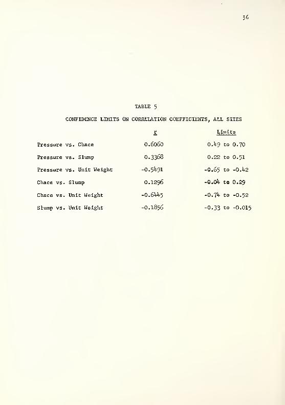
See Table 5 in the Appendix for tabulation of confidence limits on the

correlation coefficients.

26

Differences Bctr.^een Replicate Observations

As mentioned before, a time dependency was observed when the air

content was measured by the pressure meter. As a result, an analysis

of the difference between replicate observations was performed. Table 6

presents a summary of this analysis. The differences between replicate 1

and replicate 2 is significant at the 0.05 a-level for all three sites.

This is also true for the difference between replicate 1 and replicate 3«

Replicate 2 and replicate 3 difference are not significant except in

the case of Site 1 where the results are extremely close to the borderline.

These results indicate that signal change in air content occurred between

the first and second replicate.

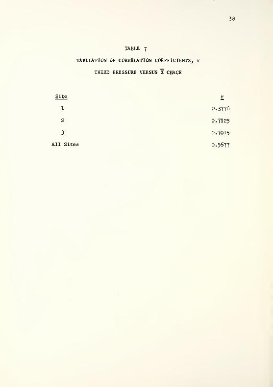
As a consequence of this finding, correlation analyses of the third

pressure reading versus the mean of the Chace meter was made. The mean

of the Chace was used since these air contents were taken immediately

after the third pressure reading and the time involved for three Chace

readings is small. The correlation coefficients for each site and over

all three sites are shown in Table "J. A comparison of these coefficients

with those of the mean pressure versus the mean Cliace show that a general

trend to a lower coefficient for the case of third pressure versus the

mean of the Chace meter reading. Considering the results of the analysis

of differences, a higher correlation could be expected. One possible

answer to the apparent contradiction is that the Chace meter air contents

are measured to only the nearest one-half percent while the pressure meter

readings are to the nearest one-tenth percent. A more realistic comparison

might be to round the pressure meter readings to the nearest one-half

percent and then make the analysis.

Basically the analysis of the differences indicates statistically

significant changes in air content measured with the pressure meter as

27

a function of time. However, the correlation of the third pressure meter

reading with the mean of the Chace meter readings is inconclusive in this

aspect of the analysis.

28

QiaLITY CONTROL APPLICATIONS

It is important to understand that a quality control system depends

upon the data used to establish the system. Control procedures therefore

are no better than the data used to establish them and it is obviously

necessary to obtain this data in some manner. There are two approaches

to this problem. One approach is to rely on past data, data collected

by examining records of construction, etc. The other approach sets out

to obtain the data required via a preliminary testing program.

There are several problems associated with using past data. One

of the most obvious is lack of reliability. The possibility is always

present that only test results that met specifications were recorded.

This situation may not arise out of desire to falsify records but rather

from a conscientious effort to maintain good control in the field. For

example, a situation may arise when something in the manufacturing process

goes awry, an acceptance test is made which detects the error and

appropriate steps are taken to correct the situation following which

another test on the product is made and recorded. The testing has served

its purpose, an error was detected and corrected, but only the last test

result recorded .

For statistical evaluation of the process, the out-of-specification

result Is just as important as the within specification result if a

realistic estimate is to be made of the variation. For this reason the

second method of obtaining the so called historical, or past data, is

used when there is a scarcity of information or there is reason to suspect

the past data. This investigation is of the second type and operated

Independent of acceptance sampling.

It should be noted at this point that there are certain limitations

associated with the results of this investigation. Only one operator and

29

one piece of testing equipment were util ized for each test method

conducted. There is, therefore, no estimate available of operator or

equipment variability. It is a recognized fact that these variables

may be significant. Another limitation arises from the fact that only

three sites were checked and these were all interstate-type construction.

In f'he preceding section entitled Analysis of Data, the measures

of central tendency and components of variability have been presented.

The problem is to now apply these results to establish a realistic

quality control program that may be implemented and used in the field.

The typical data plot in Figure 5 shows the fluctuation of the

sample means. The variability of the product, plastic portland cement

concrete, is represented by these fluctuations. One method of quality

control is to establish control limits based on the data at hand and to

use these limits to "control the quality" on future jobs. It is of no

practical value to place the calculated limits on the data plots of the

sites investigated since the calculated limits are based on the measured

variability of these sites and therefore practically all of the data

would fall within these limits.

For purposes of illustration, a variation that is considered to be

reasonable from analysis of the data will be used and the use of control

limits demonstrated in the following pages. A point should be made here

concerning the distribution of the sample means. It is possible that

the population of sample means is not normally distributed and normality

is one of the assumptions underlying the concepts of control limits. If

subgroups of U or 5 ^^e used, the central limit theorem comes into play

and the normalization effects is fairly strong. It is therefore better

at times to use "moving means" in constructing control charts.

50

There are basically three types of control charts that are of use

in the application of statistical quality control to the manufacture

of fresh portland cement concrete. These charts are the X-charts, R-chart

and the a-chart. All three of these charts provide a graphic representation

of variation from point to point (i.e., sample to sample). An objective

of using one or a combination of these charts is to keep track of the

process so that some type of corrective action may be taken whenever the

process goes "out of control" or a trend toward the control limits,

indicating the possibility that an assignable cause is adding to the

variation.

In concept, the control limits form a band within which fluctuations

in the measured values are due to random or chance variation in the process.

Observations which fall outside these limits more than a predetermined

percentage of the time cannot be explained by chance causes alone and

hence must be due to an assignable cause or a change occurring in the

process. For example, having estimates of the components of variability

associated with air content determinations, control limits may be computed

and a control chart drawn. The air contents are plotted on the chart as

the samples are tested during the manufacturing of the portland cement

concrete. As the process proceeds, it may be noted that the air contents

begin to decrease and fall outside the lower limit, hence, some assignable

cause should be responsible for this change. A check of the process may

show a defective dispenser, a change in sand gradation or some other

recognizable cause that has resulted in the process going out of control.

When this cause has been identified and corrective action taken, the

process should again come into control.

If specifications have been written so that maximum and minimum

values are given which form a band narrower than control limits based on

31

the inherent variability of the process, it will be impossible to

manufacture a product that will be within the specification all of the

time (the percentage outside will naturally depend upon specification

limits and the known standard deviation).

To illustrate one use of control limits, moving means have been

computed for the data and a plot is shown in Figure 5« The moving means

are averages of three sample means. The means of Samples 1,2 and 3 are

averaged and this is the first "moving mean." Then sample means 2, 3 and k

are averaged and this is the second moving mean. This is continued for

sample means 3> '*• and 5^ etc., and a plot of the "moving mean" is obtained.

Assumed values used in the determination of control limits are based

on the one-way ANOV and considerations of what is reasonable to expect

based on field experience. The limits are for 3-cr control limits which

would include approximately 99»T percent of data if a job were operating

in control. Note that even if a job were operating in control, 0.3^

of the data could fall outside the control limits due to chance variation

alone. If the limits were based on a 0.05 a -level, then 959^ of the data

would fall within the limits in the long run and 5^ could fall outside

the limits due to chance variation alone. This illustrates the point

that because one or two observations fall outside the control limits

does not necessarily mean process has gone "out of control."

Assuming a a_' of 0.60 for air content by pressure method, 3-0X _

control limits are: X t 1.732 (O.52) or X t O.9O. Applying these limits

to the data plot of Figure 5 it may be noted that for Site 1 about 15^

of the sample means are outside control limits hence one would conclude

that some adjustments should be made. A similar plot of the data for

Site 2 would show approximately kofo of data outside the limits. The job

Is in poor control, action should be taken. By contrast Site 3 exhibits

AIR CONTENT BY PRESSURE METER, percent

zcZwm3J

S2

r

m>

•• XII

•

1 . 1 •

'i

•

•

i 1w

1 i 1

1 1 . o1 1 o! 1

Z1 H

1 1 ^I 1 r! ! r

1 •

1 t

i *

1 *

1 •

*

1 \

MITS

1 »

•

*

\ *1 "I

O)i

1 t

i . I

i . i

1 1

( 1

1 1

i

•

•

*

»

_

»

ample

Meon

!IIIr

33

the best control, only k'^ of the data would fall outside the limits. If

the moving average concept is used, the same general conclusion may be

reached and additional information concerning trends in the data may also

be noted which may be valuable in field control.

The control limits determined from the assumed values of the

components of variation are shown on the overlay sheets for the data

plots. The 3-cf limits are in blue while the 95^ limits are not shown.

These limits are to be considered illustrative only since the variables

of operator and equipment have not been evaluated.

With estimates of the components of variance available it is

possible to take a critical look at present specifications. As mentioned

previously, even though a process is "in control" if the variability of

the process is high it may be incapable of producing a product always

inside the specification limits. If this is the case, there are several

possible avenues of action. The specifications should be examined to

determine if the limits actually need to be as tight as they are. Also,

the process itself should be examined to determine if any adjustments or

changes are possible which will reduce the inherent variability of the

process itself. This situation also points the way towards acceptance

testing. A process may be operating "in control" and still have the

product falling outside specifications. Operating "in control" does not

insure that a product will meet specifications.

There are other ways of providing control procedures and one such

method is to use tolerance limits. For example, if air content is desired

to be between ^-7^ and the variance is known, then a range of means may

be used. If the variation on a site is known and 3-cr limits determined

to be 5.55^ t 0.90^, then the average air content can be 5.5^ t 0.60^ for

a process in control and the material will meet the specified lv-7^ air

content providing the process remains in control. Another approach is

to specify a mean and allow a standard deviation range. For example,

specify a mean of 5«5^» the standard deviation may then be less than or

equal to 0.5^ for 3-ct limits and the product will pass the U-7^ specification

limits. Tables can be set up for various means and various standard

deviations, allowing a contractor operating with a known standard

deviation a certain latitude in mean air content. The same may be

accomplished by testing standard deviation and then stating that if a

standard deviation of so much is occurring then the mean air content must

be within certain limits for the product to meet specification limits.

APPENDIX

35

TABLE ^

TABUIATION OF CORREIATION COEFFICIENTS

AND SIGNIFICANCE TESTS

All Sites

Variables

Pressure v. Chace

Pressure v. Slump

Pressure v. Unit Wt.

Chace v. Slump

Chace v. Unit Wt.

Slump V. Unit Wt.

r''1U8

9.2675

*^af=0.001

3.29

Significance

0.6060 Highly Significant

0.3368 »f.35l6 3.29 Significant

O.5U9I 8.6351 3.29 Highly Significant

0.1296 1.5900 3.29 Not Significant

o.6kk3 10.25»iO 3.29 Highly Significant

0.1856 2.2977 3.29 Not Significant

Pressure v. Chace by Sites

.te r

0.5130

•"148

U. 11^05

^=0.001

3.51

Significance

1 Significant

2 0.7288 1.31^k 3.51 Highly Significant

3 0.72i^7 7.2861 3.51 Highly Significant

Interpretation of Correlation Coefficients

Correlation RelationshipCoefficient Demonstrated

1.0 Perfect0.9 Very good0.8 Good0.7 Fair0.6 Poor0.5 or less Very poor

Hughes, C. S., Enrick, N. L. and Dillard, J. H., "Applications of SomeStatistical Techniques to Experiment in Highway Engineering", VirginiaCouncil of Highway Investigations and Research in Cooperation with theU.S. Bureau of Public Roads, February 1961l-.

56

TABLE 5

CONFIDENCE LIMITS ON CORREIATION COEFFICIENTS, ALL SITES

r LjLmits

Pressure vs. Chace 0.6060 0.1^9 to 0.70

Pressure vs. Slump 0.3368 0.22 to 0.51

Pressure vs. Unit Weight -0.5^91 -0.65 to -O.U2

Chace vs. Slump 0.1296 -0,04 to 0.29

Chace vs. Unit Weight -O.6W15 -O.7I+ to -0.52

Slump vs. Unit Weight -0.1856 -0.33 to -0.015

37

TABLE 6

SUMMARY OF ANALYSIS OF DIFFERENCES

BETWEEN REPLICATE OBSERVATIONS

SITE OBSERVATION d S t-| t^ SignificantDIFFERENCE=d

S

X^ - X 0.256 0.03727 6.87 2.01 Yes

Xj - X 0.398 0.07365 5'^ 2.01 Yes

X - X O.IU2 0.07022 2.02 2.01 Yes

X^ - Xg 0.136 O.04I152 3.05 2.01 Yes

X^ - X 0.190 O.O5OU9 3.76 2.01 Yes

X - X 0.054 0.03360 1.61 2.01 No

X^ - Xg 0.208 0.03^^86 5.97 2.01 Yes

X^ - X 0.302 0.03619 6.kl 2.01 Yes

X - X 0.02i^ 0.021^7 0.97 2.01 No

58

TABLE 7

TABULATION OF CORRELATION COEFFICIENTS, r

THIRD PRESSURE VERSUS X CHACE

Site r

1 0.3776

2 0.7125

3 0.7015

All Sites 0.5677

39

BIBLIOGRAPHY

1. "Basic Statistical Methods for the Concrete Laboratory", MiscellaneousPaper No. 6-hl, Corps of Engineers, U.S. Army, Waterways ExperimentStation, October I95I (Revised June 1953).

2. Bennett, C. A. and Franklin, N. L., Statistical Analysis in Chemistryand the Chemjf'al Industry , John Wiley and Sons, Inc., 195^*

3. Burr, I. W,, Engineering Statistics and Quality Control , McGraw-Hill Book Company, Inc., 1953.

km Duncan, A. J., Quality Control and Industrial Statistics , RichardD. Irwin, Inc., 1959.

5. Grant, E. L., Statistical Quality Control , McGraw-Hill Book Company,Inc., I9I+6.

6. Hanna, S. J. and McLaughlin, J. F., "The Development of PrecisionStatements for Several ASTM Test Methods", Proc. ASTM , I963 (in Press).

7. "Highway Quality Control", Proposal for a Research Project by the

Michigan State Highway Department in Cooperation with the Bureau of

Public Roads, February I963.

8. "Highway Quality Control and Research", Fourth Annual HighwayConference, Michigan College of Mining and Technology, October 3 and k,

1963.

9. Hughes, C. S., Enrick, N. L. and Dlllard, J. H., "Applications of

Some Statistical Techniques to Experiment in Highway Engineering",Virginia Council of Highway Investigations and Research in Cooperationwith the U.S. Bureau of Public Roads, February 196k.

10. Irick, Paul, "Basic Concepts of Statistical Quality Control",Proceedings of 50th Annual Purdue Road School, March I96U.

11. "Research Project Prospectus for an Investigation of Improved QualityControl in Highway Construction", Illinois Research Suggestion No. 85,Illinois Division of Highways, Bureau of Research and Planning,March I9, I963.

12. "Statistical Methods for Quality Control of Road and Paving Materials",ASTM Special Technical Publication No. 362, June I963.