applied epidemiologic analysis fall 2002 patricia cohen, ph.d. henian chen, m.d., ph. d. teaching...

Applied Epidemiologic AnalysisFall 2002

Patricia Cohen, Ph.D.

Henian Chen, M.D., Ph. D.

Teaching Assistants

Julie Kranick Sylvia TaylorChelsea Morroni Judith Weissman

Survival Analysis


Lecture 9

Nonparametric methods to estimate the distribution of survival times (both Kaplan-Meier and life table methods)

Parametric models – Weibull model, Exponential model and Lognormal model

Semiparametric model – Cox proportional hazards model


Objectives

• To understand how to describe survival times

• To understand how to choose a survival analysis model


Survival Data (1)

Example one: Four Liver Cancer Patients

Patient Date of Diagnosis

Endpoint Date of Death or Censoring

Survival Time (Day)

Treatment

Mike 1/2/02 Dead 9/1/02 242 A

Kathy 4/7/02 Dead 7/8/02 92 A

Tom 3/3/02 Alive 11/4/02 246+ B

Susan 2/4/02 Dead 11/3/02 272 B

Complete data (noncensored data): survival time = 242, 92, 272

Incomplete data (censored data): survival time = 246+ for Tom

The survival time for Tom will exceed 246 days, but we don’t know theexact survival time for Tom.


Survival Data (2)

Right-Censored Data: Subjects observedto be event-free to a certain time beyondwhich their status is unknown

1. Subjects sometimes withdraw from a study, or die from other causes (diseases).

2. The study is completed before the endpoint is reached.

Methods for survival analysis must accountfor both censored and noncensored data.


Survival Data (3)

Survival analysis assumes censoring is random.

Censoring times vary across individuals and are not under the control of the investigator.

Random censoring also includes designs in which observation ends at the same time for all individuals, but begins at different times.


Survival Data (4)Example two: Researchers treated 65 multiple myeloma patients with alkylating agents. Of those patients, 48 died during the study and 17 survived. The goal of this study is to identify important prognostic factors.

TIME survival time in months from diagnosisSTATUS 1 = dead, 0 = alive (censored)

LOGBUN log blood urea nitrogen (BUN) at diagnosisHGB hemoglobin at diagnosisPLATELET platelets at diagnosis: 0 = abnormal, 1 = normalAGE age at diagnosis in yearsLOGWBC log WBC at diagnosisFRACTURE fractures at diagnosis: 0 = none, 1 = presentLOGPBM log percentage of plasma cells in bone marrowPROTEIN proteinuria at diagnosisSALCIUM serum calcium at diagnosis


Survival Data (5) – more examples

Survival analysis techniques arose from the life insurance industry as a method of costing insurance premiums. The term “survival” does not limit the usefulness of the technique to issues of life and death.

A “survival” analysis could be used to examine:•The survival time after a heart transplant•The time a kidney graft remains functional•The time from marriage to divorce•The time from release to first arrest•The time to a job change


Nonparametric Methods

1. Kaplan-Meier method (also called product-limit method)

2. Life table method

To estimate the distribution of survival times

-- estimate the survival rate-- calculate the median survival time-- graphs: survival curve, log(time) against log[-

log(survival rate)]-- comparison of two survival curves


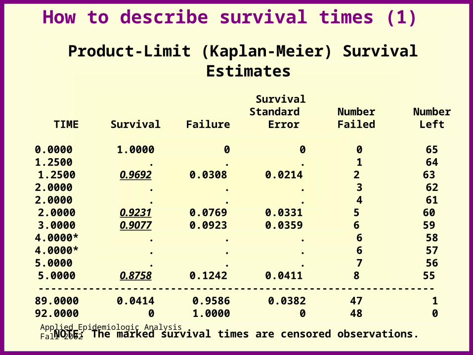
How to describe survival times (1)

Product-Limit (Kaplan-Meier) Survival Estimates

Survival Standard Number Number TIME Survival Failure Error Failed Left

0.0000 1.0000 0 0 0 651.2500 . . . 1 641.2500 0.9692 0.0308 0.0214 2 632.0000 . . . 3 622.0000 . . . 4 612.0000 0.9231 0.0769 0.0331 5 603.0000 0.9077 0.0923 0.0359 6 594.0000* . . . 6 584.0000* . . . 6 575.0000 . . . 7 565.0000 0.8758 0.1242 0.0411 8 55---------------------------------------------------------------89.0000 0.0414 0.9586 0.0382 47 192.0000 0 1.0000 0 48 0

NOTE: The marked survival times are censored observations.




ni: the number of surviving units just prior to ti

di: the number of units that fail at ti

q = di / ni

p = 1- q

time ni di q p survival rate

1.25 65 2 2/65 63/65 (63/65)=0.9692

2 63 3 3/63 60/63 (63/65)(60/63)=0.9231

3 60 1 1/60 59/60 (63/65)(60/63)(59/60)=0.9077

5 57 2 2/57 55/57 (63/65)(60/63)(59/60)(55/57)=0.8758




Kaplan-Meier method uses the actual observed event and censoring times.

A problem arises with Kaplan-Meier method if there exist censored times that are later than the last event time. The average duration will be underestimated when we use the time until the last event occurs. In the practical application of such cases, an interpretation only considers the length of time until the last event occurs.


How to describe survival times (4) Life Table Survival Estimates

Effective Conditional Interval Number Number Sample Probability [Lower, Upper) Failed Censored Size of Failure Survival NF NC n q p

0 10 16 5 62.5 0.2560 1.000010 20 15 7 40.5 0.3704 0.7440 20 30 3 1 21.5 0.1395 0.468430 40 3 0 18.0 0.1667 0.403140 50 2 1 14.5 0.1379 0.335950 60 4 2 11.0 0.3636 0.289660 70 2 0 6.0 0.3333 0.184370 80 0 1 3.5 0 0.122880 90 2 0 3.0 0.6667 0.122890 . 1 0 1.0 1.0000 0.0409

n = N – ½ (NC); 62.5 = 65 – 5/2, 40.5 = 44 – 7/2 q = NF / n; 0.2560 = 16/62.5, 0.3704 = 15/40.5p = Пp = П(1-q); 0.7440 = 1 – 0.2560, 0.4684 = (1-0.2560)(1-0.3704)



Life Table Survival Estimates

The Life Table method uses time interval.

The Life Table method is very useful for a large sample, but the estimated results will depend on the chosen interval length. The larger the interval, the poorer the estimations.

You should apply Kaplan-Meier method if the sample is not very large.



Survival Curve



Summary Statistics for Time Variable

Point 95% Confidence Interval Percent Estimate [Lower Upper)

75 52.0000 35.0000 67.0000 50 19.0000 15.0000 35.0000 25 9.0000 6.0000 14.0000

Mean Standard Error

32.1460 4.0301

Percent Total Failed Censored Censored 65 48 17 26.15



Median Survival Time

The median survival time is defined as the value at which 50% of the individuals have longer survival times and 50% have shorter survival times.

The reason for reporting the median survival time rather than the mean survival time is because the distributions of survival time data often tend to be skewed, sometimes with a small number of long-term ‘survivors’. Another reason is that we can not calculate the mean survival time for the survival time with censored data.



How to estimate median survival time

If there are no censored data, the median survival time is estimated by the middle observation of the ranked survival times.

In the presence of censored data the median survival time is estimated by first calculating the Kaplan-Meier survival curve, then finding the value of survival time when survival rate=0.50 (50%)



Graph of Log Negative Log SDF versus Log Time

Exponential DistributionThe graph is approximately a straight line, the slope is 1.

Weibull Distribution The graph is approximately a straight line, but the slope is greater or less than 1.



Graph of Log Negative Log SDF versus Log Time


Comparison of Two Survival Curves (1)



Median Survival Time

Group 1: PLATELET = 0 (abnormal)

Point 95% Confidence Interval Percent Estimate [Lower Upper) 50 13.0000 6.0000 35.0000

Group 2: PLATELET = 1 (normal)

Point 95% Confidence Interval Percent Estimate (Lower Upper) 50 24.0000 16.0000 41.0000



Test of Equality of Two Survival Curves

Test Chi-Square DF P Value Log-Rank 3.2923 1 0.0696 Wilcoxon 2.3724 1 0.1235 -2Log(LR) 2.4065 1 0.1208

Log-Rank test for Weibull distribution or proportional hazards assumption, using weight=1 so that each failure time has equal weighting, placing less emphasis on the earlier failure times.

Wilcoxon testFor lognormal distribution, using weight=the total number at risk at that time so that earlier times receive greater weight than later times, placing less emphasis on the later failure times.

-2Log(LR) : Likelihood Ratio testfor exponential distribution survival data.


Parametric Models (1)

Whenever fundamental hypotheses are to be tested or you have clear idea about the distribution of survival data, you should use a parametric model.

Three most common parametric models:

1. Exponential regression model2. Weibull regression model3. Lognormal regression model



Exponential Regression Model

The exponential distribution is a useful form of the survival distribution when the hazard function (probability of failure) is constant and does not depend on time, the graph is approximately a straight line with slope=1.

In biomedical field, a constant hazard function is usually unrealistic, the situation will not be the case.



Weibull Regression Model

The hazard function changes with time, the graph is approximately a straight line, but the slope is not 1.

The hazard function always increase when the parameter α >1

The hazard function always decrease when α <1

It is the exponential regression model when α=1



Lognormal Regression Model

The survival times are log-normal distribution.

The hazard function changes with time. The hazard function first increase and then decrease (an inverted “U” shape).


Cox Model (1)

Disadvantages of parametric models:

1. It is necessary to decide how the hazard function depends on time.

2. It may be difficult to find a parametric model if the hazard function is believed to be nonmonotonic.

3. Parametric models do not allow for explanatory variables whose values change over time. It is cumbersome to develop fully parametric models that include time-varying covariates.

Time-varying covariates are very important in survival analysis:

1) continuous time-varying variable: income is changed over time2) discrete time-varying variable: single - married - divorce - remarried


Cox Model (2)

David Cox, a British statistician, solved these problems in 1972, published a paper entitled “Regression Models and Life-Tables (with Discussion),” Journal of the Royal Statistical Society, Series B, 34:187-220

h(t|xi) = h0(t) exp (βixi)


Cox Model (3)

Why is Cox model a semiparametric model ?

h(t|xi) = h0(t) exp (βixi)

h0(t): nonparametric baseline hazard function, this function does not have to be specified, the hazard may change as a function of time.

exp (βixi): parametric form for the effects of the covariates, the hazard function changes as aexponential function of covariates


Cox Model (4)

Why is Cox model a ‘proportional hazards’ model?

Any two individuals (or groups, i & j) at any point in time, the ratio of their hazards is a constant (a fixed proportional).

For any time t, hi(t) / hj(t) = C

C may depend on explanatory variables but not on time.


Cox Model (5)

What is a partial likelihood ?

It is easy for a statistician to write down a model: h(t|xi) = h0(t) exp (βixi)

It isn’t easy to devise ways to estimate this model.

Cox’s most important contribution was to propose a method called partial likelihood because it does not include the baseline hazard function h0(t).

Partial likelihood depends only on the order in which events occur, not on the exact times of occurrence.


Cox Model (6)

What is a partial likelihood ? (cont)

Partial likelihood accounts for censored survival times.

Partial likelihood allows time-dependent explanatory variables.

It is not fully efficient because some information is lost by ignoring the exact times of event occurrence. But the loss of efficiency is usually so small that it is not worth worrying about.


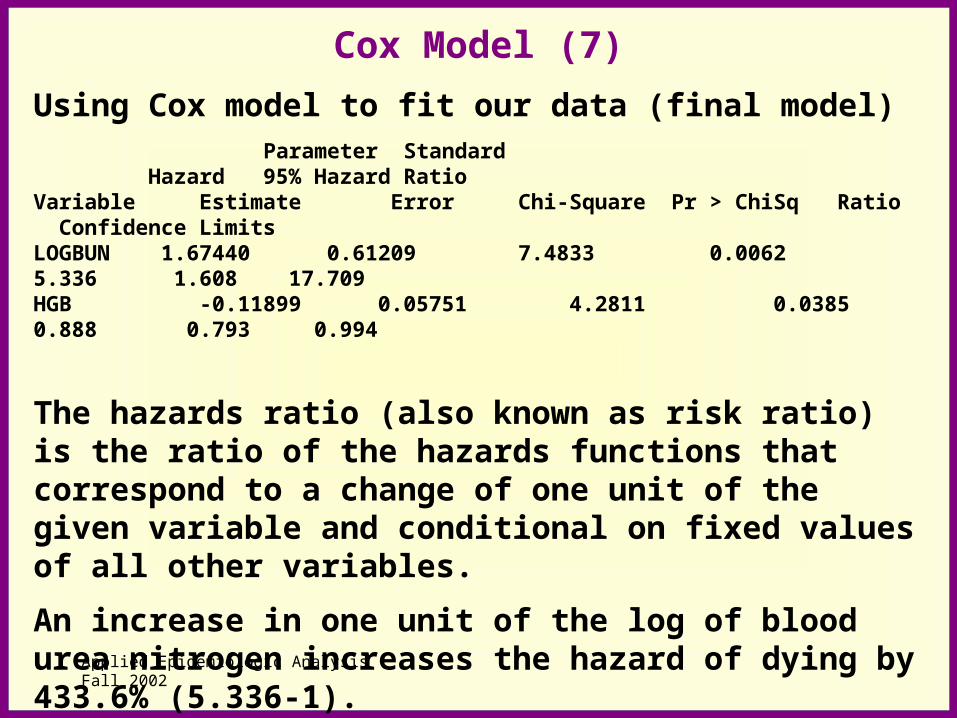
Cox Model (7)

Using Cox model to fit our data (final model) Parameter Standard Hazard 95% Hazard RatioVariable Estimate Error Chi-Square Pr > ChiSq Ratio Confidence LimitsLOGBUN 1.67440 0.61209 7.4833 0.0062 5.336 1.608 17.709HGB -0.11899 0.05751 4.2811 0.0385 0.888 0.793 0.994

The hazards ratio (also known as risk ratio) is the ratio of the hazards functions that correspond to a change of one unit of the given variable and conditional on fixed values of all other variables.

An increase in one unit of the log of blood urea nitrogen increases the hazard of dying by 433.6% (5.336-1).

An increase in one unit of hemoglobin at diagnosis decreases the hazard of dying by 11.2% (1-0.888).


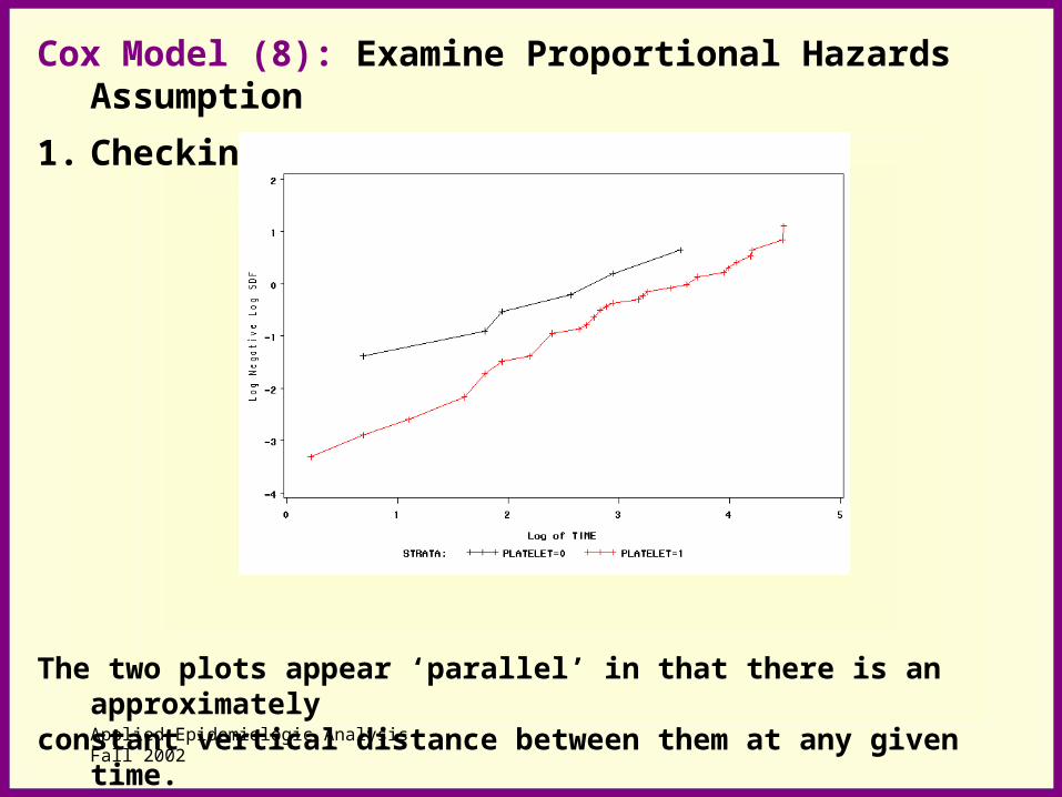
Cox Model (8): Examine Proportional Hazards Assumption

1. Checking the assumption graphically

The two plots appear ‘parallel’ in that there is an approximatelyconstant vertical distance between them at any given time.The hazards for the two groups are proportional, their ratio remainsapproximately constant with time.


Cox Model (9)

Examine Proportional Hazards Assumption cont.

2. Statistical test of the assumption

Testing the increasing or decreasing trend over time in the hazard function by investigating the interaction between time and covariate.

A significant interaction would imply the hazard function changes with time, the proportional hazards model assumption is invalid.


How do you decide which model to use? (1)

How does hazard function depend on time?

Examples

The hazard function for retirement increases with age.

The hazard function for being arrested declines with age at least after age 25.

The hazard function for death from any cause has “U” shape.



1. Using exponential regression model if hazardfunction is constant and does not depend on time.

2. Using Weibull regression model (monotonicmodels) if hazard function always increases oralways decreases with time.

3. Using Lognormal regression model(nonmonotonic models) if hazard function firstincreases and then decreases with time(an inverted “U” shape).



4. Using Cox regression model if hazard function first decreases and then increases, or changes dynamically (a “U” shape or other shapes)

Cox model can fit any distribution of survival data if the proportional hazards assumption is valid (actually most hazards ratios are fixed proportional). This is why the Cox model is used so widely now.

By the way, when we have a Cox model, we can not use this model for forecasting because we just have exp (βixi), we do not have the h0(t) (baseline hazard function).

We have to estimate h0(t) (by using BASELINE Statement in SAS) before we forecast.


Contents

1. Nonparametric methods to estimate the distribution of survival times.

2. Semiparametric model – Cox proportional hazards model.

3. Parametric models – Exponential model, Weibull model, and Lognormal model.

Objectives

1. To understand how to describe survival times.2. To understand how to choose a survival analysis

model.

applied epidemiologic analysis fall 2002 patricia cohen, ph.d. henian chen, m.d., ph. d. teaching...

Documents

median survival time

tomthe survival time

diagnosis survival data

survival curveshow

term survival

distribution of survival

functionalthe time

arrestthe time