Da

Ma

b

c

d

a

ARRAA

KDGCMS

1

dtwaatDwwd

1h

Applied Soft Computing 13 (2013) 1152–1169

Contents lists available at SciVerse ScienceDirect

Applied Soft Computing

j ourna l ho me p age: www.elsev ier .com/ l ocate /asoc

ynamic analysis and control of sieve tray gas absorption column using MATALBnd SIMULINK

enwer Attarakiha,c,∗, Mazen Abu-Khaderb, Hans-Jörg Bartc,d

The University of Jordan, Faculty of Eng. & Tech., Chem. Eng. Department, 11942 Amman, JordanAl-Balqa Applied University, Faculty of Eng. & Tech., Chem. Eng. Department, P.O. Box 15008, 11134 Amman, JordanTU Kaiserslautern, Chair of Separation Science and Technology, P.O. Box 3049, 67653 Kaiserslautern, GermanyTU Kaiserslautern, Centre of Mathematical and Computational Modelling, P.O. Box 3049, 67653 Kaiserslautern, Germany

r t i c l e i n f o

rticle history:eceived 16 November 2011eceived in revised form 19 February 2012ccepted 23 October 2012vailable online 12 November 2012

eywords:ynamic modellingas absorptionontrolATLAB

IMULINK

a b s t r a c t

The present work highlights the powerful combination of SIMULINK/MATLAB software as an effectiveflowsheeting tool which was used to simulate steady state, open and closed loop dynamics of a sieve traygas absorption column. A complete mathematical model, which consists of a system of differential andalgebraic equations was developed. The S-Functions were used to build user defined blocks for steadystate and dynamic column models which were programmed using MATLAB and SIMULINK flowsheet-ing environment. As a case study, the dynamic behaviour and control of a sieve tray column to absorbethanol from CO2 stream in a fermentation process were analysed. The linear difference equation relat-ing the actual and equilibrium gas phase compositions was solved analytically to relate the actual gasphase composition to the liquid phase with Murphree tray efficiency as a parameter. The steady statemathematical model was found to be nonlinear (w.r.t. number of stages) due to the introduction of theMurphree tray efficiency. To avoid the solution of large linear algebraic system, a sequential steady statesolution algorithm was developed and tested through the idea of tearing the recycle stream in the closedloop configuration. The number of iterations needed to achieve a given tolerance was found to be functionof the Murphree tray efficiency. The open-loop dynamic analysis showed that the gas phase compositionresponse was nonlinear with respect to the inlet gas flow rate, while it was linear with respect to inlet gas

composition. The nonlinearity increased along the column height and was maximum at the top tray. Onthe other hand, the Murphree tray efficiency had little effect on the dynamic behaviour of the column. Thecontrolled variable was found to exhibit fairly large overshoots due to step change in the inlet gas flowrate, while the PID controller performance was satisfactory for step change in the inlet gas composition.The closed-loop dynamic analysis showed that the controlled variable (outlet gas phase composition)had a fairly linear dynamics due to step changes in the set point.

. Introduction

Steady state design of chemical equipment is confronted byynamic and controllability issues. In this regard, it is often easyo design a chemical process based on steady state conditions,hich is practically uncontrollable and unrealistic. In order to

void any wrong assumption during process synthesis and design,nd to ensure safe start-up, shutdown and stable plant operation,he dynamic behaviour of the relevant units should be known.ynamic simulation is known to be a slow process, in particular

hen used on the flowsheet level, where the challenge is dealingith processing units having different time constants. However,ynamic simulation makes use of recent advances in computers

∗ Corresponding author.E-mail address: m.attarakih@ju.edu.jo (M. Attarakih).

568-4946/$ – see front matter © 2012 Elsevier B.V. All rights reserved.ttp://dx.doi.org/10.1016/j.asoc.2012.10.011

© 2012 Elsevier B.V. All rights reserved.

power in terms of memory and computational speed, and theadvances in information technology where user friendly GUI andflowsheeting packages are used intensively [1,2,21,28,29]. Kvams-dal et al. [2] presented three important factors, which contributeto the importance of the dynamic simulation to improve the over-all design and optimize the operation of chemical processing units.These factors are: (1) the coupled absorber/stripper system is com-plex, with higher degree of two-way interaction between these twounits. (2) The upstream processing units might operate under avarying load operation. (3) New process approaches, with energyintegration mean more complex operations. Therefore, a dynamicprocess simulator enables the study of most of these isolated orcoupled effects.

The dynamic simulation and control of gas absorption processattracted many researchers’ attention on both individual and flow-sheet (planwide) levels [2,3,28,29]. Kvamsdal et al. [2] presenteda dynamic model of a CO2 absorption column that is intended to

M. Attarakih et al. / Applied Soft Com

Nomenclature

AP active plate area (m2)b slope of equilibrium curvec weir constant (m1/2 s−1)G gas flow rate (mol/s)Gc industrial PID controller transfer function (psig)hw weir height (m)K equilibrium constantKc controller gainKp process gain (s/mol)L0 absorbent inlet flow rate (mol/s)Lw weir length (m)Lj liquid flow rate from the jth tray (mol/s)Mj total liquid holdup on jth tray (kmol)M0 steady state liquid holdup on each tray (kmol)N number of traysP column operating pressure (atm)T column operating temperature (◦C)t time (s)xin, yin solute mole fraction in the inlet absorbent and gas

stream respectivelyx steady state mole fraction of solute concentration in

the liquid phasexj mole fraction of solute in the liquid phasey∗

jis the equilibrium solute mole fraction in the gasphase leaving stage j

yj mole fraction of solute in the gas phase leaving stagej

Greek symbols˛ parameter introduced to realize the controller

transfer function�I, �D integral and derivative actions respectively (s)

bcIatpwTuatma

puptcppHrr

ac

� Murphree tray efficiency�L molar density of the liquid mixture (mol/m3)

e coupled with models of other individual processes to form aomplete model of a power generation plant with CO2 removal.n their model, the operational challenges, such as load variationnd high degree of heat integration between the power plant andhe absorber/stripper process were studied. Lin et al. [3] presentedlanwide control of a reactive CO2 absorption/stripping processith monoethanol-amine as a solvent using dynamic simulation.

hese authors proposed a new control structure, where the liq-id absorbent flow rate (at the top of the column), the liquid levelnd temperature at the bottom of the stripping column were con-rolled. Through the help of dynamic simulations, the developed

odel and control structure was found to achieve removal targetsnd stabilize quickly under the influence of external disturbances.

Robinson and Luyben [28,29] presented a hybridower/chemical plant model for the purpose of dynamic sim-lation and planwide control structure design. This hybridower/chemical plant is the gasification process producing syn-hesis gas, which under standard operation conditions feed aombustion turbine to generate electricity or feed a chemicallant during periods of lower power demand. These authors usedrocess simulator ASPEN to perform dynamic simulations of the2S and CO2 absorption/stripping processes and water–gas shift

eactors, which are essential for the development of stable and

obust plantwide control structures of this hybrid plant.

From the above review, it is obvious that dynamic simulationnd control of gas absorption process is essential. Moreover, it islear that gas absorption/stripping is one of the main and important

puting 13 (2013) 1152–1169 1153

processing blocks in many chemical and power generation plants.It is used in pollution control devices such as wet scrubbers andspray-dryer-type, dry scrubbers for the removal of acid gas com-pounds and water-soluble organic compounds [4,5]. This processis usually carried out through tray columns that contain multiplenumbers of trays, which bring gas and liquid into intimate contact.If the gas leaving the tray is in thermodynamic equilibrium (whichis a rather rare situation) with the liquid leaving the tray, thentheoretical stage is provided. To account for the failure to achieveequilibrium, Murphree tray efficiency is used. The computationalapproach is to determine the theoretical stages and then correct toactual stages by means of tray efficiency [6]. The use of the com-ponent Murphree tray efficiency for separation of binary mixtureshas been described by several authors: Hines and Maddox [7], VanWinkle [8], Edmister [9] and Holland and McMahon [10]. However,a simple way to apply Murphree tray efficiency to liquid–vapourseparation processes has not been shown. Edmister [9] presenteda description of different types and uses of tray efficiencies. A trayefficiency was defined as a multiplier of the absorption or strip-ping factor on each stage. Takamatsu and Kinoshita [11] showeda new solution process for multi-component distillation columns.They took the liquid mole fractions to be the independent variablesand their difference between consecutive iterations to be the func-tions set to zero. Their procedure seems to be stable and fast, andthe application of the Murphree efficiency includes a new step insolving the liquid–vapor composition non-equilibrium equationswith a successive substitution method. In general, the values of theMurphree tray efficiencies are not equal throughout the column.Further, they usually are not equal for the different components ina mixture, even on the same stage.

The gas absorption process is modelled through a systemof mathematical equations to enable prediction of the processbehaviour [12]. These equations do not have a general analyticalsolution and some approximations and numerical methods canbe used for solving them [13]. The implementation of a controlscheme for such a process is vital to achieve optimal operationdespite the presence of significant uncertainty about the plantbehaviour and disturbances. The purpose of any control systemis to suppress the influence of external disturbances, ensure thestability of process and optimize process performance. The feed-back system is a common control configuration where it uses directmeasurements of the controlled variables to adjust the values ofthe manipulated variables. The objective is to keep the controlledvariables at desired levels (set points) [14,15]. There are vari-ous controllers that can be considered for implementation suchas: proportional–integral–derivative (PID) controller and ArtificialNeural Networks (ANN) controller [16]. As the capability of a certaincontroller is not the main issue of the present work, the traditionalPID controller was selected for its simplicity when compared withANN and being able to achieve the required targets. Tuning the PIDfeedback controllers is the adjustment of the controller parame-ters to match the characteristics of the rest of the components ofthe loop. One of the popular methods is the on-line or closed-looptuning method. For the desired response of the closed loop, Zieglerand Nichols specified a decay ratio of one-fourth. The decay ratio isthe ratio of the amplitudes of two successive oscillations ([17,18]).

MATLAB is a software for mathematical computation, whereasSIMULINK is a powerful software for modelling, simulation, andanalysis of dynamical systems in a flowsheeting environment. Itsupports linear and nonlinear systems, modelled in continuoustime, sampled time, or a hybrid of the two. Bequette [19], illus-trated that the interactive MATLAB/SIMULINK tool enhances the

ability to learn new model-based techniques and provide an insidedepth of the dynamic nature and control of chemical processes [20].For modelling, SIMULINK provides a graphical user interface (GUI)for building models as block diagrams, using click-and-drag mouse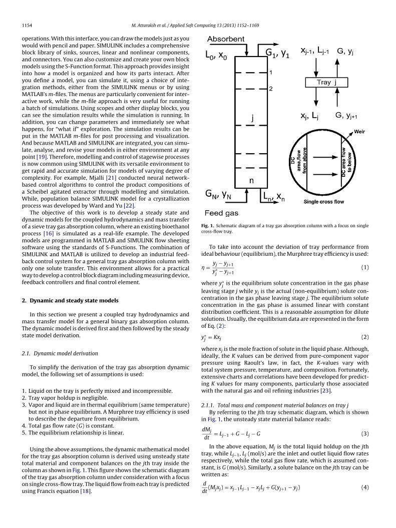

1 ft Computing 13 (2013) 1152–1169

owbamiygMaacahpAlpigcbaWp

dopmsSbowf

2

mTs

2

m

123

45

ftcoou

154 M. Attarakih et al. / Applied So

perations. With this interface, you can draw the models just as youould with pencil and paper. SIMULINK includes a comprehensive

lock library of sinks, sources, linear and nonlinear components,nd connectors. You can also customize and create your own blockodels using the S-Function format. This approach provides insight

nto how a model is organized and how its parts interact. Afterou define a model, you can simulate it, using a choice of inte-ration methods, either from the SIMULINK menus or by usingATLAB’s m-files. The menus are particularly convenient for inter-

ctive work, while the m-file approach is very useful for running batch of simulations. Using scopes and other display blocks, youan see the simulation results while the simulation is running. Inddition, you can change parameters and immediately see whatappens, for “what if” exploration. The simulation results can beut in the MATLAB m-files for post processing and visualization.nd because MATLAB and SIMULINK are integrated, you can simu-

ate, analyse, and revise your models in either environment at anyoint [19]. Therefore, modelling and control of stagewise processes

s now common using SIMULINK with its versatile environment toet rapid and accurate simulation for models of varying degree ofomplexity. For example, Mjalli [21] conducted neural network-ased control algorithms to control the product compositions of

Scheibel agitated extractor through modelling and simulation.hile, population balance SIMULINK model for a crystallization

rocess was developed by Ward and Yu [22].The objective of this work is to develop a steady state and

ynamic models for the coupled hydrodynamics and mass transferf a sieve tray gas absorption column, where an existing bioethanolrocess [16] is simulated as a real-life example. The developedodels are programmed in MATLAB and SIMULINK flow sheeting

oftware using the standards of S-Functions. The combination ofIMULINK and MATLAB is utilized to develop an industrial feed-ack control system for a general tray gas absorption column withnly one solute transfer. This environment allows for a practicalay to develop a control block diagram including measuring device,

eedback controllers and final control element.

. Dynamic and steady state models

In this section we present a coupled tray hydrodynamics andass transfer model for a general binary gas absorption column.

he dynamic model is derived first and then followed by the steadytate model derivation.

.1. Dynamic model derivation

To simplify the derivation of the tray gas absorption dynamicodel, the following set of assumptions is used:

. Liquid on the tray is perfectly mixed and incompressible.

. Tray vapor holdup is negligible.

. Vapor and liquid are in thermal equilibrium (same temperature)but not in phase equilibrium. A Murphree tray efficiency is usedto describe the departure from equilibrium.

. Total gas flow rate (G) is constant.

. The equilibrium relationship is linear.

Using the above assumptions, the dynamic mathematical modelor the tray gas absorption column is derived using unsteady stateotal material and component balances on the jth tray inside the

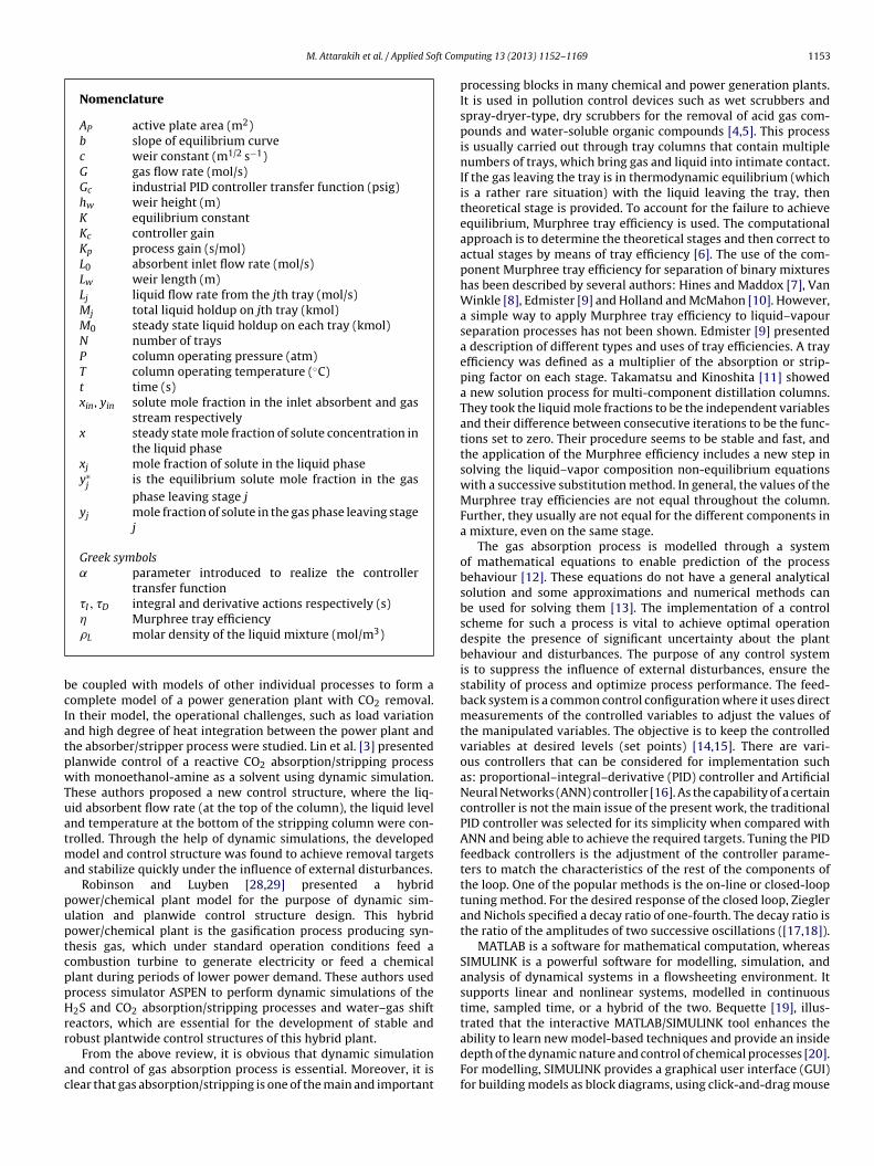
olumn as shown in Fig. 1. This figure shows the schematic diagramf the tray gas absorption column under consideration with a focusn single cross-flow tray. The liquid flow from each tray is predictedsing Francis equation [18].

Fig. 1. Schematic diagram of a tray gas absorption column with a focus on singlecross-flow tray.

To take into account the deviation of tray performance fromideal behaviour (equilibrium), the Murphree tray efficiency is used:

� = yj − yj+1

y∗j

− yj+1(1)

where y∗j

is the equilibrium solute concentration in the gas phaseleaving stage j while yj is the actual (non-equilibrium) solute con-centration in the gas phase leaving stage j. The equilibrium soluteconcentration in the gas phase is assumed linear with constantdistribution coefficient. This is a reasonable assumption for dilutesolutions. Usually, the equilibrium data are represented in the formof Eq. (2):

y∗j = Kxj (2)

where xj is the mole fraction of solute in the liquid phase. Although,ideally, the K values can be derived from pure-component vaporpressure using Raoult’s law, in fact, the K-values vary withtotal system pressure, temperature, and composition. Fortunately,extensive charts and correlations have been developed for predict-ing K values for many components, particularly those associatedwith the natural gas and oil refining industries [23].

2.1.1. Total mass and component material balances on tray jBy referring to the jth tray schematic diagram, which is shown

in Fig. 1, the unsteady state material balance reads:

dMj

dt= Lj−1 + G − Lj − G (3)

In the above equation, Mj is the total liquid holdup on the jthtray, while Lj−1, Lj (mol/s) are the inlet and outlet liquid flow ratesrespectively, while the total gas flow rate, which is assumed con-

stant, is G (mol/s). Similarly, a solute balance on the jth tray can bewritten as:

d

dt(Mjxj) = xj−1Lj−1 − xjLj + G(yj+1 − yj) (4)

M. Attarakih et al. / Applied Soft Computing 13 (2013) 1152–1169 1155

S-1

Gas absorption column

Feed backcontroler

S-3

Contro lvalve

Manipulated variablesL0

Unmeasured variable ....,,121

yyy N 1

yy outN y(control variable)

Disturbances

yin xinG

M. D.

gas analyzer

feedba

wpb

2

tmtt

L

wai

o

y

wtt(iwNendE

aim

Desired set poin t

Fig. 2. Typical block flow diagram for the

here xj and yi are the solute mole fractions in the liquid and gashases respectively. The tray index j runs from 1 (top tray) to n (theottom) tray.

.1.2. Tray fluid dynamicsFrom dynamic point of view, the liquid flow rates throughout

he column will not be the same. They will depend on the fluidechanics of the tray. Often a simple Francis weir formula rela-

ionship is used to relate the liquid holdup on the jth tray (Mj) tohe liquid flow rate leaving the tray (L) [24]:

j = �LLw

[1c

(Mj

�LAp− hw

)]3/2

(5)

here hw is weir height (m), Lw is weir length (m), Ap is active platerea (m2), �L is the molar density of the liquid mixture (mol/m3), cs a weir empirical constant (m−1/3 s2/3).

The Murphree tray efficiency can be written explicitly in termsf the equilibrium solute mass fraction y∗

jas follows:

j = (1 − �)N+1−jyin + �y∗j + �

N−j−1∑m=0

(1 − �)N−j−my∗N−m (6)

here j = 1, 2, . . . , N. Note that when � → 1, yj → y∗j

and hencehe ideal tray model is recovered. In the above equation the firsterm is the solution of the homogeneous finite difference equationEq. (1)), while the second two terms are the particular solution. Its clear that the first term accounts for the inlet boundary condition,

hich is required to solve the Murphree finite difference equation.ote that all the terms in Eq. (6) are nonlinear with respect to trayfficiency (�), except the second term. The second two terms areonlinear with respect departure of the tray from equilibrium con-itions. The derivation of Eq. (6) as a solution to the finite differenceq. (1) is shown in Appendix A.

It is obvious that the above system of equations is a differentiallgebraic equation (DAE) system, which can be solved sequentiallyn time thanks to the explicit form of Eq. (6). Note that the solute

ole fraction yj in Eq. (4) can be eliminated using Eqs. (6) and (2),

ck control of tray gas absorption column.

which results in a system of ODE in terms of solute mole fraction(x) in the liquid phase.

2.1.3. Initial conditionsThe initial conditions for the system of Eqs. (3) and (4) are given

by the solution of the steady state versions of these equations. Theinitial conditions can be stated mathematically as:

Mj(0) = M0,j

Lj(0) = L0,j

xj(0) = x0,j

yj(0) = y0,j

∀j = 1, 2, . . . , N (7)

To examine the system degrees of freedom, the feed gas flowrate (G) and its inlet composition (yin) are assumed to be givenfrom the upstream unit. The Murphree tray efficiency is assumedto be known empirically. The total number of variables is equalto 5N + 2 and the total number of equations is 5 N. From controlengineering point of view, there are only two variables that can becontrolled. These two variables are the inlet absorbent flow rate andcomposition. The inlet absorbent composition (xin) is specified fromthe upstream unit (stripper or distillation column) and hence it is adisturbance imposed on the process. Accordingly, we are left onlywith the absorbent flow rate (L0) as a manipulated variable. Theabsorbent flow rate is manipulated using a feedback controller tocontrol the composition of the gas stream leaving the top of the trayabsorption column as shown in Fig. 2. This adds an extra equation toclose the dynamic model. The equation should relate the absorbentflow rate to the gas stream composition leaving the column usingthe feedback (PID) controller equation:

L0(t) = f (yN) (8)

Fig. 2 shows the block diagram of the controlled gas absorptioncolumn with total inlet gas flow rate (G), composition (yin) and theinlet absorbent composition (xin) as the main three disturbances tothe closed loop control system. The controlled (measured) variable

1 ft Com

ic

2

dpap

A

wm

A

(

(

B

v

Lic

2

cpai

(a′x)i,j =

⎡⎢⎢⎣

−(

Lj

Mj+ 1

m

dMj

dt

), if i = j

Lj

⎤⎥⎥⎦ ,

156 M. Attarakih et al. / Applied So

s the gas outlet concentration leaving the top tray (yN), which isontrolled by manipulating the absorbent flow rate (L0).

.2. Steady state model derivation

The steady state model of the tray gas absorption column iserived using the steady state versions of Eqs. (3) and (4) cou-led with the algebraic system given by Eq. (6), where Lj−1 = Lj = Lt steady state. For ease of presentation, the steady state model isut in compact matrix form as follows:

xx = Bu − �y (9)

The above equation is a result of combining Eqs. (3) and (4),hile the Murphree tray efficiency (Eq. (6)) is expressed in compactatrix form as follows:

yy = −�Kx − (1 − �)yinv (10)

In the above equations, the elements of Ax and Ay are given by:

ax)i,j =

⎡⎢⎣ −

(L0

G

)if i = j

−(

L0

G

)if j = i + 1

⎤⎥⎦ , ∀i, j = 1, 2, . . . , N

ay)i,j =[

−1 if i = j

1 − � if j = i + 1

], ∀i, j = 1, 2, . . . , N

While the elements of the vectors B, u, �y, v and y are given by:

=

⎡⎢⎢⎢⎢⎣

−1 0

0 0

.. ..

.. ..

0 −1

⎤⎥⎥⎥⎥⎦ , u =

⎡⎣ L0

Gxin

yin

⎤⎦ ,

�y =

⎡⎢⎢⎢⎢⎢⎢⎢⎢⎣

�y1

�y2

..

..

�yN−1

−yN

⎤⎥⎥⎥⎥⎥⎥⎥⎥⎦

, �yj = yj+1 − yj, j = 1, 2, . . . , N

=

⎡⎢⎢⎢⎢⎢⎢⎣

0

0

..

..

0

1

⎤⎥⎥⎥⎥⎥⎥⎦

, x =

⎡⎢⎢⎢⎢⎢⎢⎢⎢⎣

x1

x2

..

..

xN−1

xN

⎤⎥⎥⎥⎥⎥⎥⎥⎥⎦

, y =

⎡⎢⎢⎢⎢⎢⎢⎢⎢⎣

y1

y2

..

..

yN−1

yN

⎤⎥⎥⎥⎥⎥⎥⎥⎥⎦

Note that the system input variables (the manipulated variable:0 and the disturbances: G, xin and yin) are all contained in thenput vector u, while the system outputs (the liquid and gas phaseompositions) are contained in the vectors: x and y respectively.

.2.1. Steady state solution algorithmThe steady state system of equations given by (9) and (10) is

oupled through the vectors x and y due to the presence of Mur-hree tray efficiency (�). When � = 1 (ideal tray) the two systemsre decoupled and a sequential solution of the two linear systemss allowed.

puting 13 (2013) 1152–1169

This decomposed system consists of two parts: the x-phase andthe y-phase systems, where each of them has an N × N dimension.On the other hand, the coupled system of linear equations has adimension of 2N × 2N. This results in the solution of large and denselinear system, which is undesirable from numerical point of view.Fig. 3 presents the conceptual flow diagram of the coupled systemin both closed loop and cycle tearing configurations. This is to high-light the sequential solution algorithm of this system. By doing this,an efficient iterative solution algorithm is developed. The algorithmstarts by neglecting the correction terms (the two nonlinear terms)in Eq. (6) to get the following approximation:

y = �y∗ (11)

Moreover, by dropping the (1 − �) term from Eq. (10) one getsAyy = �Kx, where the matrix Ay = I (I is the identity matrix). Accord-ingly, using the last result, the vector �y in Eq. (9) becomes �y =�K�x. Substituting this in Eq. (9) to get Axx + �K�x = Bu, whichcan be written in a more compact way to solve for the initial guessvector (x0):

Ax0 = Bu (12)

Due to the appearance of the vector �K�x, the elements of thematrix A are given by:

(a)i,j =

⎡⎢⎣ −

(�K + L0

G

), if i = j

L0

Gif i = j + 1

⎤⎥⎦

And the elements of B and u are the same as those given byEq. (9). The steady state solution algorithm can be summarized asfollows:1 Solve the system: Ax0 = Bu to get the initial guess x0.2 Calculate the vector y by solving the system: Ayy = −�Kx − 1(1 − �)inv.3 Calculate the new vector x by solving the system: Axx = Bu − �y.4 Check for convergence: error = ||x − x0||.5 if (error < Tolerance) then

STOPelsex = x0

GOTO STEP 2End if

2.3. Dynamic model derivation and solution algorithm

After expanding the derivative vector on the left hand side ofEq. (4), the dynamic model given by Eqs. (3)–(5) is cast into the fol-lowing state-space form, which is suitable for MATLAB/SIMULINKimplementation:

dx

dt= A′

xx + A′yy + B′u (13)

where the elements of A′x and A′

y are given by:

Miif i = j + 1

j = 1, 2, . . . , N, u′

[xin

yin

]

M. Attarakih et al. / Applied Soft Computing 13 (2013) 1152–1169 1157

F ecove

(

i

atccast

Mtp

ig. 3. (a) The conceptual flow diagram of the closed loop coupled system and (b) r

a′y)

i,j=

⎡⎢⎢⎣

−(

G

Mj

), if j = i

G

Miif j = i + 1

⎤⎥⎥⎦ ,

= 1, 2, . . . , N, B′

⎡⎢⎢⎢⎢⎢⎢⎣

L0

M10

0 0...

...

0G0

MN

⎤⎥⎥⎥⎥⎥⎥⎦

,dMj

dt= Lj−1 − Lj

nd y is given by the solution of Eq. (6) or (10). Note that the DAE sys-em above, which results from the slow dynamics of the tray liquidomposition (dx/dt) and the negligible dynamics of the gas phaseomposition (dy/dt ≈ 0) is represented by the two state variables xnd y which are transformed by the matrices A′

x and A′y, while the

ystem disturbances and manipulated variables are augmented inhe vector B′u.

The dynamic solution algorithm starts by filling the trays withj kmol liquid (absorbent) followed by solving the steady state sys-

em given by Eqs. (9) and (10) using the algorithm of Section 2.2.1 torovide an initial condition to the dynamic model. Then, the system

ring the sequential solution by tearing the recycle and adding a convergence block.

of ODEs given by Eq. (13) is integrated using the standard MATLABordinary differential Equation solvers.

It is interesting to explore again the nonlinear structure of thedynamic model by examining the elements of the governing matri-ces in the system of Eq. (13). The matrices A′

x, A′y and B′ are functions

of time and space (stage number) due to the coupled mass transferprocess and tray hydrodynamics. This is exacerbated by the nonlin-ear behaviour of the equilibrium gas phase mole fraction as functionof liquid tray composition, which is reflected by Eq. (6). This non-linearity is expected to propagate along the column height evenwhen the system attains its steady state value due the appearanceof the fractional efficiency � in Eq. (6). For ideal tray (� = 1) thegas phase composition is given in Eq. (2) with constant equilib-rium constant (K). This reduces the right hand side of the dynamicmodel (13) to [A′

x + KA′]x + B′u. Since the two matrices A′x and A′

yare both bidiagonal, then the eigenvalues of [A′

x + KA′y] are simply

the diagonal elements, which are given by �i = (a′x)i,i + (a′

y)i,i

< 0.This insures the stability of the dynamic model (13). Moreover, thespeed of response is controlled by the system time constants, whichare given by = �i = [(a′

x)i,i + (a′y)

i,i]−1. This shows that the depend-

ence of the time constants on the gas and liquid flow rates, thedynamic tray holdup and the equilibrium distribution coefficient(K). Therefore, the ideal sieve tray absorption column is expectedto show a nonlinear dynamic behaviour characterized by variable

1158 M. Attarakih et al. / Applied Soft Computing 13 (2013) 1152–1169

Tray absorption colum n

AIC101

AT101

AY101

inx0L

outyG

outxL

inyG

Fermentation t anks Absorbent + alcohol

Gas mixture (CO2 + a lcohol)

Absorbent (water)Effluent gas

PID Controller

(a)

inxL ,0 outyG,

outxL,inyG,

Absorbent

+ alcohol

Gas mixture

(CO2 + alcohol)

Absorbent

(water)

Effluent

gas

Gas absorptio n

column

(b)

(b) th

t(tAmaea

3c

aaFta

Fig. 4. (a) The complete bioethanol process [16] and

ime constants. This variability depends on the absorbent flow rateL) and the gas phase flow rate (G). For the general case (nonidealray), the matrix A′

y in Eq. (13) is modified by the elements of the−1y as a solution to the system of Eq. (10). This results in new ele-ents which are functions of � and K. Since these two parameters

re considered constant, one expect no effect on the system nonlin-arity, which is inherited to the try hydrodynamic model as shownbove.

. MATLAB/SIMULINK software: control of gas absorptionolumn

To highlight the applicability of the developed steady statend dynamic solution algorithms, a real industrial bioethanol gas

bsorption process is chosen as a case study [16]. By referring toig. 4, this process is described as follows: The collected gas mix-ure (CO2 + ethanol) from the sugarcane fermentation tanks is fedt the bottom and the absorbent liquid at the top of the ethanol

e input–output structure of the absorption column.

recovery column, where the two phases flow counter currently.A distillation column supplies the absorbent liquid, consisting ofwater containing some alcohol (around 100 ppm). This absorptioncolumn is composed of nine stages and operates at 40 ◦C and 1 atm.This equipment must process 3 mol/s of gas mixture in order toreduce the alcohol concentration from approximately 20,000 to300 ppm.

The initial concentration depends on the fermentation brothconditions and also on specific features of the fermentation tanks.Therefore, this is considered as a disturbance to the absorption pro-cess and the absorbent flow rate must be manipulated to maintaina high ethanol recovery. The effluent gas from the first column,mainly composed of carbon dioxide, a small amount of ethanol,and around 2000 ppm of water, is fed into a depurator to oxidizethe organic impurities. A 10-tray absorption column is then used to

reduce the water concentration in the gas mixture to 300 ppm. Thecontrol purpose is: to keep low ethanol concentration in the efflu-ent gas phase from the first absorption column (ethanol recoverycolumn) despite the changes in the two main disturbances: the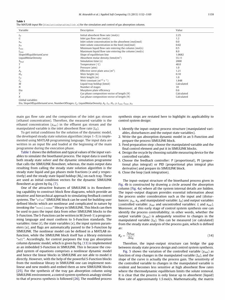

M. Attarakih et al. / Applied Soft Computing 13 (2013) 1152–1169 1159

Table 1The MATLAB input file (SimulationDataSimulink.m) for the simulation and control of gas absorption column.

Variable Description Value

L0 Initial absorbent flow rate (mol/s) 2.25G Inlet gas flow rate (mol/s) 1.2xin Inlet solute concentration in the absorbent (mol/mol) 0.0yin Inlet solute concentration in the feed (mol/mol) 0.02Lmin Minimum liquid flow rate entering the column (mol/s) 0.5Lmax Maximum liquid flow rate entering the column (mol/s) 8.0SlopeOfEquilibriumCurve Slope of equilibrium line 1.0682LiquidMolarDensity Absorbent molar density (kmol/m3) 55.11Tfinal Simulation time (s) 2000T Temperature (◦C) 40.0P Pressure (atm) 1.0Ap Effective sieve plate area (m2) 1.21Hw Weir height (m) 0.10Lw Weir length (m) 1.0Cp Weir constant (m1/2 s−1) 1.848M Liquid tray holdup (kmol) CalculatedN Number of stages 10Eta Murphree plate efficiency 0.6Y Gas phase composition vector of length (N) CalculatedX Gas phase composition vector of length (N) Calculated

w , y, L

m(em

tmwp

abtrstafl

iisdibSmveSf“capadfl[St

Global variablesEta, SlopeOfEquilibriumCurve, NumberOfStages, Cp , LiquidMolarDensity, Ap , Lw , H

ain gas flow rate and the composition of the inlet gas streamethanol concentration). Therefore, the measured variable is thethanol concentration (yout) in the effluent gas stream and theanipulated variable is the inlet absorbent flow rate (L0).To get initial conditions for the solution of the dynamic model,

he developed steady state solution algorithm (steps 1–5) is imple-ented using MATLAB programming language. The input data areritten in an input file and loaded at the beginning of the mainrogramme during the execution phase.

Table 1 shows the definition and typical values of the input vari-bles to simulate the bioethanol process. The input data is used byoth steady state solver and the dynamic simulation programmehat calls the SIMULINK flowsheet, whereas, the main output dataesulting from calling the steady state solution algorithm is theteady state liquid and gas phases mole fractions (x and y respec-ively) and the steady state liquid holdup (M0) on each tray. Thesere used as initial condition vectors for the dynamic SIMULINKowsheet as given by Eq. (7).

One of the attractive features of SIMULINK is its flowsheet-ng capability to construct block flow diagrams, which provide anntuitive and hierarchical approach to simulating feedback controlystems. The “sfun” SIMULINK block can be used for building userefined blocks which are nonlinear and complicated in nature by

nvoking the “nonlinear” library in SIMULINK. This block can thene used to pass the input data from other SIMULINK blocks to the-Function. The S-Function can be written in M (level-1) a program-ing language and must conform to S-Function standards. The

ariables: time (t), the state variables (x), the input system param-ters (u), and flags are automatically passed to the S-Function byIMULINK. The nonlinear model can be defined in a MATLAB m-unction, while the SIMULINK block itself has a library extensionmdl”. Accordingly, for control purposes the tray gas absorptionolumn dynamic model, which is given by Eq. (13) is implementeds an imbedded S-Function in SIMULINK. This is because the cou-led system of equations comprises a nonlinear dynamic modelnd hence the linear blocks in SIMULINK are not able to model itirectly. However, with the help of the powerful S-Function blocksrom the nonlinear library in SIMULINK one can implement non-

inear and new models and embed them as new SIMULINK blocks25]. For the synthesis of the tray gas absorption column usingIMULINK environment, a control system synthesis analogy similaro that of process synthesis is followed [26]. The modified process

min, Lmax, yin

synthesis steps are restated here to highlight its applicability tocontrol system design:

1. Identify the input–output process structure (manipulated vari-ables, disturbances and the output state variables).

2. Write the gas absorption dynamic model in an S-Function andprepare the process SIMULINK block.

3. Feed preparation step: choose the manipulated variable and thefinal control element and put it in SIMULINK blocks.

4. Design the recycle by choosing suitable measuring device for thecontrolled variable.

5. Choose the feedback controller: P (proportional), PI (propor-tional plus integral) or PID (proportional plus integral plusderivative) and prepare its SIMULINK block.

6. Close the loop (task integration).

The input–output structure of the bioethanol process given inFig. 4b is constructed by drawing a circle around the absorptioncolumn (Fig. 4a) where all the system internal details are hidden.The input–output diagram provides essential information aboutthe process under consideration such as the input and (distur-bances: yin, xin and manipulated variable: L0) and output variables(controlled variable: yout and uncontrolled variables: L and xout).Moreover, at this early stage of control system synthesis one canidentify the process controllability; in other words, whether theoutput variable (yout) is adequately sensitive to changes in themanipulated variable (L0). This can be measured (or calculated)from the steady state analysis of the process gain, which is definedas:

Kp = �yout

�L0(14)

Therefore, the input–output structure can bridge the gapbetween steady state process design and control system synthesis.

Fig. 5 shows the variation of the controlled variable (yout) asfunction of step changes in the manipulated variable (L0), and theslope of the curve is actually the process gain. The sensitivity ofthe controlled variable to changes in the manipulated variable is

evident and becomes less sensitive at high absorbent flow rateswhere the thermodynamic equilibrium limits the solute removal.It is clear that the process is only linear up to absorbent (liquid)flow rate of approximately 1.5 mol/s. Mathematically, the matrix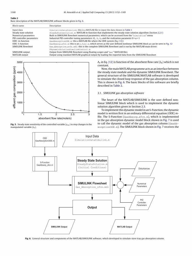

1160 M. Attarakih et al. / Applied Soft Computing 13 (2013) 1152–1169

Table 2Basic description of the MATLAB/SIMULINK software blocks given in Fig. 6.

Block name Description

Input data SimulationDataSimulink: this is a MATLAB file to input the data shown in Table 1Steady state solution SteadyStatesolution.m: MATLAB m-function that implements the steady state solution algorithm (Section 2.2.1)Numerical parameters Built in SIMULINK flowsheet numerical parameters, which can be accessed from the “simulation” menuPID controller parameters Industrial PID controller tuning parameters: Kc , �I , �D and the realization parameter 0 < ̨ < 1ODE: m-function GasAbsorptionODE.m: this a MATLAB file where the ODE system (Eq. (13))ODE: S-function GasAbsorp sfcn.m: this is an s func.m, which serves as the user defined nonlinear SIMULINK block as can be seen in Fig. 12SIMULINK flowsheet Gas Absorption scfn.mdl: this is the complete SIMULINK flowsheet and is run by the MATLAB main driver:

FDynamicSolutionSimulinkControl.m

SIMULINK output Output from SIMULINK flowsheet using floating sMATLAB output Output using standard MATLAB graphical output

1 1. 5 2 2. 5 30

1000

2000

3000

4000

5000

absorbent flow rate(mole/s)

eff

lue

nt g

as c

om

po

sitio

n (

pp

m)

Fig. 5. Steady state sensitivity of the controlled variable (yout) to step changes in themanipulated variable (L0).

Input DataSimulationDataSi

Steady State SoSteadyStateSolu(Initial Condi

SIMULINK FlowGas_Absorption_s

S-Function

GasAbsorp_sfcn.m

ODE

GasAbsorptionODE.m

Output

SIMULINK Output

Fig. 6. General structure and components of the MATLAB/SIMULINK softw

copes and “mat” MATLAB filesby loading the exported data from the SIMULINK flowsheet

Ax in Eq. (12) is function of the absorbent flow rate (L0) which is notconstant.

Now, the main MATLAB programme acts as an interface betweenthe steady state module and the dynamic SIMULINK flowsheet. Thegeneral structure of the SIMULINK/MATLAB software is developedto simulate the closed loop response of the gas absorption column.This is shown in Fig. 6. The basic blocks of this software are brieflydescribed in Table 2.

3.1. SIMULINK gas absorption software

The heart of the MATLAB/SIMULINK is the user defined non-linear SIMULINK block which is used to implement the dynamicsolution algorithm given in Section 2.3.

To implement this dynamic model in an S-Function, the dynamicmodel is written first in an ordinary differential equation (ODE) m-

file. The S-Function (GasAbsorp sfcn.m), which is implementedin the gas absorption dynamic model block shown in Fig. 7 is usedto call the dynamic model of the gas absorption column (GasAb-sorptionODE.m). The SIMULINK block shown in Fig. 7 receives the

mulink.m

lutiontion.mtions)

sheetfcn.mdl

Disturbances

Numerical

Parameters

PID

Controller

Parameters

MATLAB Output

are, which developed to simulate sieve tray gas absorption column.

M. Attarakih et al. / Applied Soft Computing 13 (2013) 1152–1169 1161

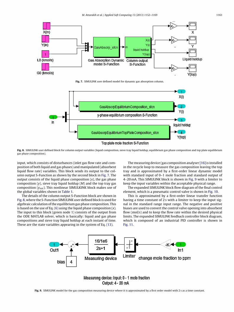
Fig. 7. SIMULINK user defined model for dynamic gas absorption column.

F n, sievg

ipluocct

FaiTtcT

ig. 8. SIMULINK user defined block for column output variables (liquid compositioas phase composition).

nput, which consists of disturbances (inlet gas flow rate and com-osition of both liquid and gas phases) and manipulated (absorbent

iquid flow rate) variables. This block sends its output to the col-mn output S-Function as shown by the second block in Fig. 7. Theutput consists of the liquid phase composition (x), the gas phaseomposition (y), sieve tray liquid holdup (M) and the top tray gasomposition (yout). This nonlinear SIMULKINK block makes use ofhe global variables shown in Table 1.

The details of the column output S-Function block are shown inig. 8, where the S-Function SIMULINK user defined block is used forlgebraic calculation of the equilibrium gas phase composition. Thiss based on the use of Eq. (6) using the liquid phase composition (x).

he input to this block (green node 1) consists of the output fromhe ODE MATLAB solver, which is basically: liquid and gas phaseompositions and sieve tray liquid holdup at each instant of time.hese are the state variables appearing in the system of Eq. (13).

Fig. 9. SIMULINK model for the gas composition measuring device where

e tray liquid holdup, equilibrium gas phase composition and top plate equilibrium

The measuring device (gas composition analyser [16] is installedin the recycle loop to measure the gas composition leaving the toptray and is approximated by a first-order linear dynamic modelwith standard input of 0–1 mole fraction and standard output of4–20 mA. This SIMULINK block is shown in Fig. 9 with a limiter tokeep the input variables within the acceptable physical range.

The expanded SIMULINK block flow diagram of the final controlelement, which is a pneumatic control valve is shown in Fig. 10.

This is approximated by a first-order linear transfer functionhaving a time constant of 2 s with a limiter to keep the input sig-nal in the standard range input range. The negative and positivebiases are used to convert the control valve opening into absorbent

flow (mol/s) and to keep the flow rate within the desired physicallimits. The expanded SIMULINK feedback controller block diagram,which is composed of an industrial PID controller is shown inFig. 11.

it is approximated by a first order model with 2 s as a time constant.

1162 M. Attarakih et al. / Applied Soft Computing 13 (2013) 1152–1169

Fig. 10. SIMULINK model for pneumatic control valve, where it is modelled as a first order system with time constant equals to 3 s.

indust

t

G

wtt0tib

a

Fd

Fig. 11. SIMULINK model for industrial PID controller. In this example the

An industrial version of the PID controller is used here to realizehe controller transfer function that is given by:

c(S) = Kc�Is + 1

�Is

�Ds + 1˛�Ds + 1

(15)

here Kc is the controller gain, �I and �D are the integral and deriva-ive actions respectively. The parameter ̨ is introduced to realizehe controller transfer function and has a value that ranges from.05 to 0.2 [18]. These parameters can be adjusted by the user fromhis SIMULINK subsystem. Note that the PID controller built block

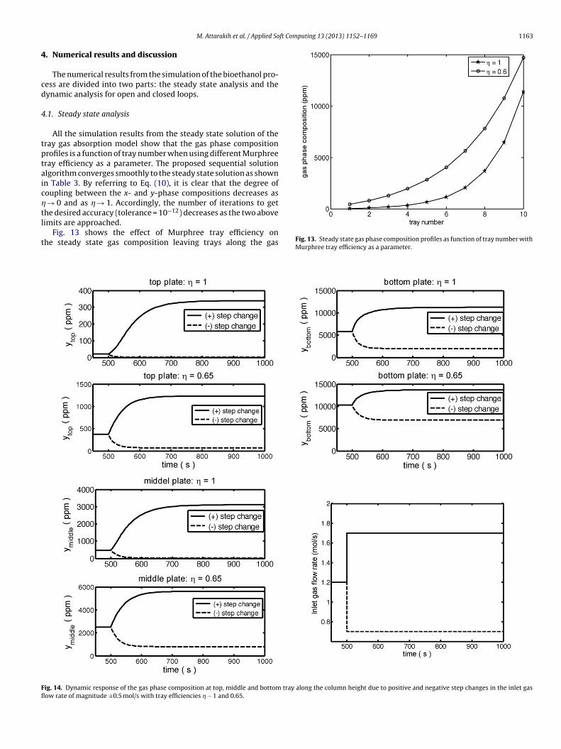
n SIMULINK does not support the industrial PID controller giveny Eq. (15).

Now, all the major elements in the closed control loop of Fig. 2re modelled using SIMULINK. The last step in the control system

ig. 12. SIMULINK model for a closed loop gas absorption column where the gas absorpefined S-Functions and nonlinear SIMULINK blocks.

rial controller adjustable parameters are: �I = 8.5 s, �D = 2.1 s and ̨ = 0.05 s.

synthesis is the task integration, where all the elements are wiredtogether using the SIMULINK flowsheeting environment. Fig. 12shows the complete SIMULINK flowsheet of the gas absorption pro-cess, with source and sink blocks to facilitate data input and output.The main inputs to the control system are the disturbances in inletgas flow rate, composition and the set point. These are accom-plished by SIMULINK step change blocks, where the step changemagnitude, direction (positive or negative) and the time at whichthe step change begins can be easily set by the user in the SIMULINKflowsheet. These inputs are recorded as a function of time by sav-ing their data to a MATLAB formatted data files. These data are then

loaded and plotted using MATLAB. On the other hand, the floatingscope SIMULINK block can be used as recorders for the data outputat any point along the directed edges as shown in Fig. 12.

tion dynamic model (GasAbsorp sfcn block) and its output are created using user

ft Computing 13 (2013) 1152–1169 1163

4

cd

4

tptaic�tl

t

Ffl

M. Attarakih et al. / Applied So

. Numerical results and discussion

The numerical results from the simulation of the bioethanol pro-ess are divided into two parts: the steady state analysis and theynamic analysis for open and closed loops.

.1. Steady state analysis

All the simulation results from the steady state solution of theray gas absorption model show that the gas phase compositionrofiles is a function of tray number when using different Murphreeray efficiency as a parameter. The proposed sequential solutionlgorithm converges smoothly to the steady state solution as shownn Table 3. By referring to Eq. (10), it is clear that the degree ofoupling between the x- and y-phase compositions decreases as

→ 0 and as � → 1. Accordingly, the number of iterations to get

he desired accuracy (tolerance = 10−12) decreases as the two aboveimits are approached.

Fig. 13 shows the effect of Murphree tray efficiency onhe steady state gas composition leaving trays along the gas Fig. 13. Steady state gas phase composition profiles as function of tray number with

Murphree tray efficiency as a parameter.

ig. 14. Dynamic response of the gas phase composition at top, middle and bottom tray along the column height due to positive and negative step changes in the inlet gasow rate of magnitude ±0.5 mol/s with tray efficiencies � − 1 and 0.65.

1164 M. Attarakih et al. / Applied Soft Computing 13 (2013) 1152–1169

F tray

c

aptttapsrpE

TNo

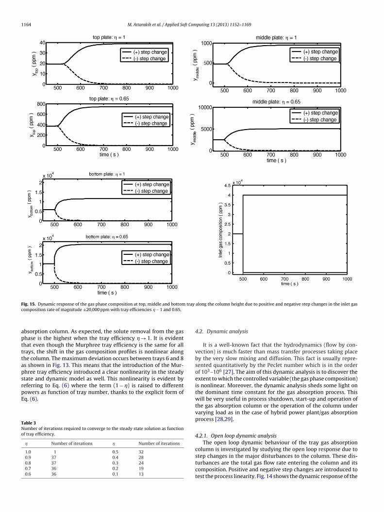
ig. 15. Dynamic response of the gas phase composition at top, middle and bottomomposition rate of magnitude ±20,000 ppm with tray efficiencies � − 1 and 0.65.

bsorption column. As expected, the solute removal from the gashase is the highest when the tray efficiency � → 1. It is evidenthat even though the Murphree tray efficiency is the same for allrays, the shift in the gas composition profiles is nonlinear alonghe column. The maximum deviation occurs between trays 6 and 8s shown in Fig. 13. This means that the introduction of the Mur-hree tray efficiency introduced a clear nonlinearity in the steadytate and dynamic model as well. This nonlinearity is evident by

eferring to Eq. (6) where the term (1 − �) is raised to differentowers as function of tray number, thanks to the explicit form ofq. (6).

able 3umber of iterations required to converge to the steady state solution as functionf tray efficiency.

� Number of iterations � Number of iterations

1.0 1 0.5 320.9 37 0.4 280.8 37 0.3 240.7 36 0.2 190.6 36 0.1 13

along the column height due to positive and negative step changes in the inlet gas

4.2. Dynamic analysis

It is a well-known fact that the hydrodynamics (flow by con-vection) is much faster than mass transfer processes taking placeby the very slow mixing and diffusion. This fact is usually repre-sented quantitatively by the Peclet number which is in the orderof 103–106 [27]. The aim of this dynamic analysis is to discover theextent to which the controlled variable (the gas phase composition)is nonlinear. Moreover, the dynamic analysis sheds some light onthe dominant time constant for the gas absorption process. Thiswill be very useful in process shutdown, start-up and operation ofthe gas absorption column or the operation of the column undervarying load as in the case of hybrid power plant/gas absorptionprocess [28,29].

4.2.1. Open loop dynamic analysisThe open loop dynamic behaviour of the tray gas absorption

column is investigated by studying the open loop response due to

step changes in the major disturbances to the column. These dis-turbances are the total gas flow rate entering the column and itscomposition. Positive and negative step changes are introduced totest the process linearity. Fig. 14 shows the dynamic response of the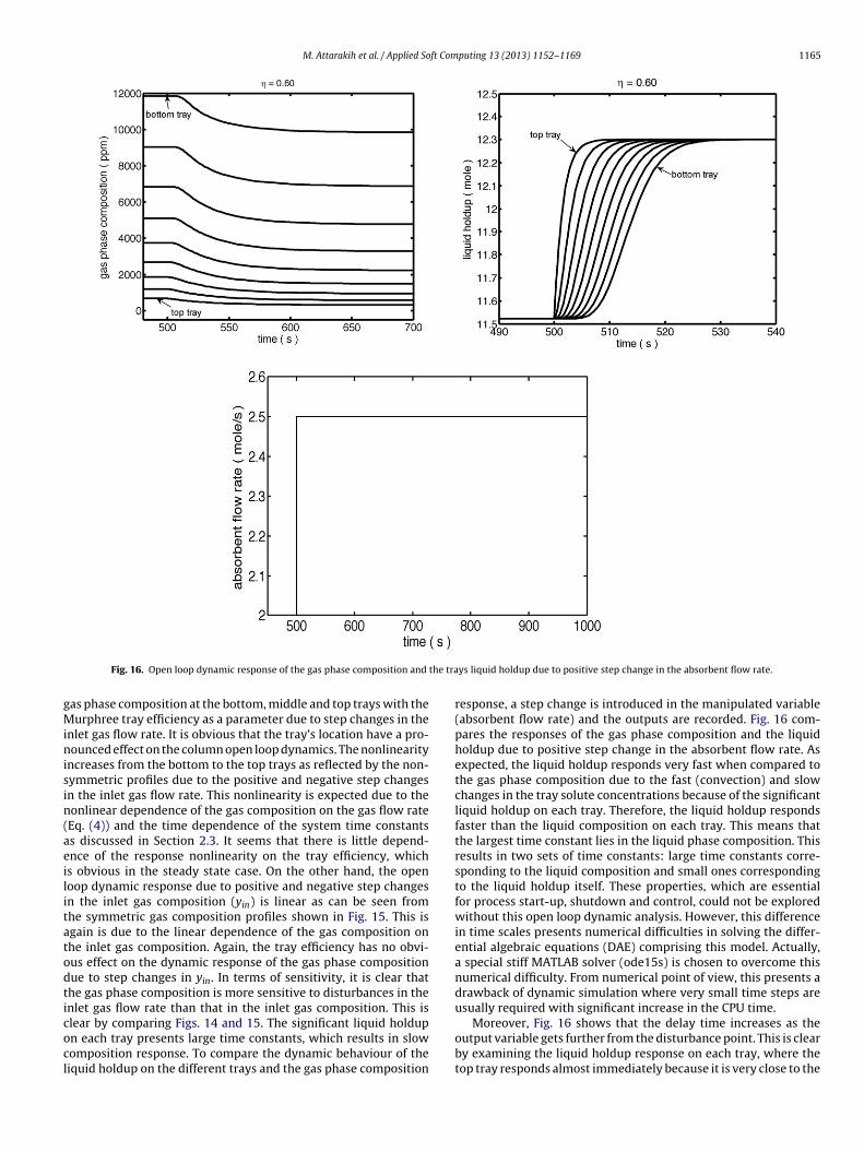

M. Attarakih et al. / Applied Soft Computing 13 (2013) 1152–1169 1165

the tra

gMinisin(aeilitatodticocl

Fig. 16. Open loop dynamic response of the gas phase composition and

as phase composition at the bottom, middle and top trays with theurphree tray efficiency as a parameter due to step changes in the

nlet gas flow rate. It is obvious that the tray’s location have a pro-ounced effect on the column open loop dynamics. The nonlinearity

ncreases from the bottom to the top trays as reflected by the non-ymmetric profiles due to the positive and negative step changesn the inlet gas flow rate. This nonlinearity is expected due to theonlinear dependence of the gas composition on the gas flow rateEq. (4)) and the time dependence of the system time constantss discussed in Section 2.3. It seems that there is little depend-nce of the response nonlinearity on the tray efficiency, whichs obvious in the steady state case. On the other hand, the openoop dynamic response due to positive and negative step changesn the inlet gas composition (yin) is linear as can be seen fromhe symmetric gas composition profiles shown in Fig. 15. This isgain is due to the linear dependence of the gas composition onhe inlet gas composition. Again, the tray efficiency has no obvi-us effect on the dynamic response of the gas phase compositionue to step changes in yin. In terms of sensitivity, it is clear thathe gas phase composition is more sensitive to disturbances in thenlet gas flow rate than that in the inlet gas composition. This is

lear by comparing Figs. 14 and 15. The significant liquid holdupn each tray presents large time constants, which results in slowomposition response. To compare the dynamic behaviour of theiquid holdup on the different trays and the gas phase composition

ys liquid holdup due to positive step change in the absorbent flow rate.

response, a step change is introduced in the manipulated variable(absorbent flow rate) and the outputs are recorded. Fig. 16 com-pares the responses of the gas phase composition and the liquidholdup due to positive step change in the absorbent flow rate. Asexpected, the liquid holdup responds very fast when compared tothe gas phase composition due to the fast (convection) and slowchanges in the tray solute concentrations because of the significantliquid holdup on each tray. Therefore, the liquid holdup respondsfaster than the liquid composition on each tray. This means thatthe largest time constant lies in the liquid phase composition. Thisresults in two sets of time constants: large time constants corre-sponding to the liquid composition and small ones correspondingto the liquid holdup itself. These properties, which are essentialfor process start-up, shutdown and control, could not be exploredwithout this open loop dynamic analysis. However, this differencein time scales presents numerical difficulties in solving the differ-ential algebraic equations (DAE) comprising this model. Actually,a special stiff MATLAB solver (ode15s) is chosen to overcome thisnumerical difficulty. From numerical point of view, this presents adrawback of dynamic simulation where very small time steps areusually required with significant increase in the CPU time.

Moreover, Fig. 16 shows that the delay time increases as theoutput variable gets further from the disturbance point. This is clearby examining the liquid holdup response on each tray, where thetop tray responds almost immediately because it is very close to the

1166 M. Attarakih et al. / Applied Soft Computing 13 (2013) 1152–1169

500 503 506 509 512 515 518 521 524 527 530 533 536 539 542 545 548 551 554 557 560350

360

370

380

390

400

410

420

430

440

450

460

time ( s )

y top (

ppm

)

controlled variableset point

Ku = -9000 P

u

F1a

a(

4

e(ctcpdhavtu(

c−ca

upstActtbct

TBu

490 500 510 520 530 540 550 56012

12.1

12.2

12.3

12.4

12.5

12.6

12.7

12.8

12.9

13

liqu

id h

old

up

(m

ole

)

time ( s )

top tray

bottom tray

change in the inlet gas flow rate is characterized by large overshootsaround the set point as can be seen in Fig. 20. This is due to the highsensitivity of the gas phase composition to the inlet gas flow rate.

480 500 520 540 560 580 600395

400

405

410

415

y top (

pp

m)

controlled variableset point

3.5

4

x 104

ition (

ppm

)

time (s)

ig. 17. The ultimate controller gain (Ku = −9000) and period of oscillation (Pu =7 s) using the continuous cycling method applied to the closed-loop tray gasbsorption column.

bsorbent inlet. This is one of the main characteristics of stagewiseor distributed) systems [1,18].

.2.2. Closed loop dynamic analysisThe closed loop dynamic behaviour is investigated in the pres-

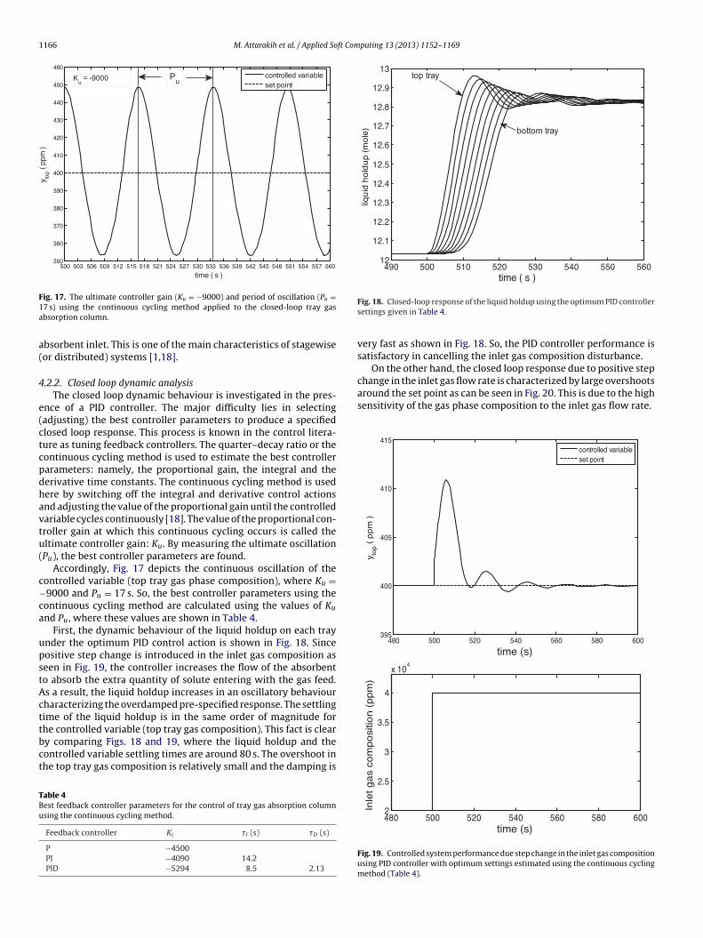
nce of a PID controller. The major difficulty lies in selectingadjusting) the best controller parameters to produce a specifiedlosed loop response. This process is known in the control litera-ure as tuning feedback controllers. The quarter–decay ratio or theontinuous cycling method is used to estimate the best controllerarameters: namely, the proportional gain, the integral and theerivative time constants. The continuous cycling method is usedere by switching off the integral and derivative control actionsnd adjusting the value of the proportional gain until the controlledariable cycles continuously [18]. The value of the proportional con-roller gain at which this continuous cycling occurs is called theltimate controller gain: Ku. By measuring the ultimate oscillationPu), the best controller parameters are found.

Accordingly, Fig. 17 depicts the continuous oscillation of theontrolled variable (top tray gas phase composition), where Ku =9000 and Pu = 17 s. So, the best controller parameters using the

ontinuous cycling method are calculated using the values of Ku

nd Pu, where these values are shown in Table 4.First, the dynamic behaviour of the liquid holdup on each tray

nder the optimum PID control action is shown in Fig. 18. Sinceositive step change is introduced in the inlet gas composition aseen in Fig. 19, the controller increases the flow of the absorbento absorb the extra quantity of solute entering with the gas feed.s a result, the liquid holdup increases in an oscillatory behaviourharacterizing the overdamped pre-specified response. The settlingime of the liquid holdup is in the same order of magnitude for

he controlled variable (top tray gas composition). This fact is cleary comparing Figs. 18 and 19, where the liquid holdup and theontrolled variable settling times are around 80 s. The overshoot inhe top tray gas composition is relatively small and the damping is

able 4est feedback controller parameters for the control of tray gas absorption columnsing the continuous cycling method.

Feedback controller Kc �I (s) �D (s)

P −4500PI −4090 14.2PID −5294 8.5 2.13

Fig. 18. Closed-loop response of the liquid holdup using the optimum PID controllersettings given in Table 4.

very fast as shown in Fig. 18. So, the PID controller performance issatisfactory in cancelling the inlet gas composition disturbance.

On the other hand, the closed loop response due to positive step

480 500 520 540 560 580 6002

2.5

3

Inle

t gas

com

pos

time (s)

Fig. 19. Controlled system performance due step change in the inlet gas compositionusing PID controller with optimum settings estimated using the continuous cyclingmethod (Table 4).

M. Attarakih et al. / Applied Soft Computing 13 (2013) 1152–1169 1167

490 500 510 520 530 540 550 560340

360

380

400

420

440

460

480

500

520

time (s)

time (s)

y top (

ppm

)

controlled variableset point

490 500 510 520 530 540 550 5601

1.5

2

2.5

Inle

t ga

s flo

w r

ate

( m

ole

/s)

Fig. 20. Controlled system performance due step change in the inlet gas flow rateusing PID controller with optimum settings estimated using the continuous cyclingmethod (Table 4).

490 500 510 520 530 540 550 560 570400

450

500

550

600

time (s)

time (s)

y top (

ppm

)

controlled variableset point

500 520 540 560200

250

300

350

400

450

y top (

ppm

)

controlled variableset point

Fig. 21. Controlled system performance due to positive and negative step changesin the set point using PID controller with optimum settings estimated using thecontinuous cycling method (Table 4).

500 520 540 560 580300

350

400

450

500

550

time ( s )

y top (

ppm

)

controlled variableset point

Fig. 22. Controlled system performance due simultaneous positive step changes in

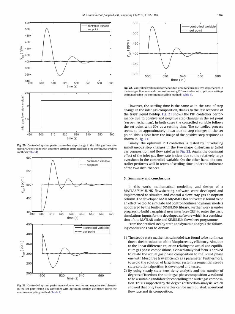
the inlet gas flow rate and composition using PID controller with optimum settingsestimated using the continuous cycling method (Table 4).

However, the settling time is the same as in the case of stepchange in the inlet gas composition, thanks to the fast response ofthe trays’ liquid holdup. Fig. 21 shows the PID controller perfor-mance due to positive and negative step changes in the set point(servo-mechanism). In both cases the controlled variable followsthe set point with 60 s as a settling time. The controlled processseems to be approximately linear due to step changes in the setpoint. This is clear from the image of the positive step response asshown in Fig. 21.

Finally, the optimum PID controller is tested by introducingsimultaneous step changes in the two major disturbances (inletgas composition and flow rate) as in Fig. 22. Again, the dominanteffect of the inlet gas flow rate is clear due to the relatively largeovershoot in the controlled variable. On the other hand, the con-troller performs well in terms of settling time under the influenceof the two disturbances.

5. Summary and conclusions

In this work, mathematical modelling and design of aMATLAB/SIMULINK flowsheeting software were developed andimplemented to simulate and control a sieve tray gas absorptioncolumn. The developed MATLAB/SIMULINK software is found to bean effective tool to simulate and control nonlinear dynamic modelsnot offered by the built-in SIMULINK library. Further work is underprogress to build a graphical user interface (GUI) to enter the basicsimulations inputs for the developed software which is a combina-tion of the MATLAB code and SIMULINK flowsheet programme.

From the detailed steady state and dynamic analysis the follow-ing conclusions can be drawn:

1) The steady state mathematical model was found to be nonlineardue to the introduction of the Murphree tray efficiency. Also, dueto the linear difference equation relating the actual and equilib-rium gas phase compositions, a closed analytical form is derivedto relate the actual gas phase composition to the liquid phaseone with Murphree tray efficiency as a parameter. Furthermore,to avoid the solution of large linear system, a sequential steadystate solution algorithm is developed and tested.

2) By using steady state sensitivity analysis and the number ofdegrees of freedom, the outlet gas phase composition was foundto be a suitable candidate for controlling the outlet gas composi-

tion. This is supported by the degrees of freedom analysis, whichshowed that only two variables can be manipulated: absorbentflow rate and its composition.

1 ft Com

3

4

5

6

A

t

At

fi

(

•

•

•

[

[

[

[

[

[

[

[

[

168 M. Attarakih et al. / Applied So

) The dynamic model was characterized by two sets of timeconstants: the smallest time was associated with tray hydro-dynamics, while the larger one was related to the change inthe gas phase composition. Accordingly, special MATLAB ODEsolver was used (ode15s) to integrate the open and closed loopmodels.

) The open-loop dynamic analysis showed that the gas phasecomposition response is nonlinear with respect to the inlet gasflow rate, while it was linear with respect to inlet gas composi-tion. The nonlinearity increases along the column height and itwas found to be maximum at the top tray. On the other hand,the Murphree tray efficiency had little effect on the dynamicbehaviour of the column.

) The closed-loop dynamic analysis showed that the controlledvariable (outlet gas phase composition) had a fairly lineardynamics due to step changes in the set point.

) The continuous cycling method was used to estimate the PIDcontroller parameters for the control of the bioethanol gasabsorption column. The controlled variable was found to exhibitfairly large overshoots due to step change in the inlet gas flowrate, while the PID controller performance was satisfactory forstep change in the inlet gas composition.

cknowledgments

The authors are very grateful to the German Research Associa-ion (DFG) for the financial support.

ppendix A. Derivation of the gas phase composition inerms of tray efficiency

The tray efficiency as given by Eq. (1) can be put in the standardnite difference form:

1 − �)yj+1 − yj + �y∗j = 0 (A-1)

Now, take N = 5 to get:

j = 5

ys = (1 − �)y6 + �y∗s

ys = (1 − �)yin + �y∗s

j = 4

y4 = (1 − �)ys + �y∗4 = (1 − �)[(1 − �)yin + �y∗

s ] + �y∗4

y4 = (1 − �)2yin + (1 − �)(�)y∗s + �y∗

4

j = 3

y3 = (1 − �)y4 + �y∗3

= (1 − �)[(1 − �)2yin + (1 − �)(�)y∗5 + �y∗

5 + �y∗4] + �y∗

3

y3 = (1 − �)3yin + (1 − �)2(�)y∗s + (1 − �)(�)y∗

4 + �y∗3

[

[

[

[

[

[

puting 13 (2013) 1152–1169

• j = 2

y2 = (1 − �)y3 + �y∗2

y2 = (1 − �)[(1 − �)3]yin + (1 − �)2(�)y∗5

+ (1 − �)�y∗4 + �y∗

4 + �y∗3 + �y∗

3 + �y∗2]

y3 = (1 − �)4yin + (1 − �)3(�)y∗5

+ (1 − �)2(�)y∗4 + (1 − �)1(�)y∗

4 + (1 − �)(�)y∗3 + �y∗

3

So, one can generalize to get Eq. (6):

yj = (1 − �)N+1−jyin + �y∗j +

N−j−1∑m=0

(1 − �)N−m−jy∗N−M (A-2)

References

[1] M. Attarakih, M. Jaradat, H. Allaboun, H.-J. Bart, N. Faqir, Dynamic modelingof a rotating disk contactor using the primary and secondary particle method(PSPM), in: B. Braunschweig, X. Joulia (Eds.), Escape, vol. 18, Elsevier, Lyon,France, 2008.

[2] H.M. Kvamsdal, J.P. Jakobsen, K.A. Hoff, Dynamic modeling and sim-ulation of a CO2 absorber column for postcombustion CO2 capture,Chemical Engineering and Processing: Process Intensification 48 (2009)135–144.

[3] Y. Lin, T. Pan, D. Wong, S. Jang, Y. Chi, C. Yeh, Plantwide controlof CO2 capture by absorption and stripping using monoethanolaminesolution, Industrial and Engineering Chemistry Research 50 (3) (2010)1338–1345.

[4] R.G. Griskey, Transport Phenomena and Unit Operations a Combined Approach,John Wiley & Sons, Inc., New York, 2002.

[5] R. Treybal, Mass Transfer Operations, McGraw-Hill Book Co., Singapore, 1981.[6] L.F. Albright, Albright’s Chemical Engineering Handbook, CRC Press, New York,

2009.[7] A.L. Hines, R.N. Maddox, Mass Transfer Fundamentals and Applications,

Prentice-Hall, NJ, 1985.[8] M. Van Winkle, Distillation, McGraw Hill, NY, 1967.[9] W.C. Edmister, Hydrocarbon absorption and fractionation process

design methods. Part 18. Tray efficiency, The Petroleum Engineer, C-45,January extraction contactors, Chemical Engineering Science 60 (1949)239–253.

10] C.D. Holland, K.S. McMahon, Comparison of vaporization efficiencies withMurphree-type efficiencies in distillation – I, Chemical Engineering Science 25(1970) 431–436.

11] T. Takamatsu, M. Kinoshita, A simulation procedure for multi component distil-lation columns incorporating tray efficiencies, Journal of Chemical Engineeringof Japan 18 (1) (1985) 78–81.

12] W. McCabe, J. Smith, P. Harriout, Unite Operation of Chemical Engineering, 7thed., McGraw Hill, Singapore, 2005.

13] D. Prieve, Unit Operation of Chemical Engineering, Carnegie Mellon University,Pittsburgh, USA, 2000.

14] H. Dag-Kjetil, Dynamic modeling of an absorption tower, M.Sc. thesis, TelemarkUniversity College, 2004.

15] A. Aroonwilas, A. Chakma, P. Tontiwaxhwuthikul, A. Veawab, Mathemat-ical modeling of mass-transfer, Chemical Engineering Science 58 (2003)4037–4053.

16] E. Eyng, A. Fileti, Control of absorption columns in the bioethanol process:influence of measurement uncertainties, Engineering Applications of ArtificialIntelligence 23 (2) (2010) 271–282.

17] G. Stephanopoulos, Chemical Process Control, Prentice Hall, Englewood Cliffs,NJ, 1983.

18] C. Smith, A.B. Corripio, Principles and Practice of Automatic Process Control,3rd ed., John Wiley & Sons, Inc., New York, 2006.

19] B.W. Bequette, Process Control: Modeling, Design and Simulation, Prentice Hall,Upper Saddle River, NJ, 2003.

20] D. Seborg, D. Mellichamp, T. Edgar, F. Doyle, Process Dynamics and Control, 3rded., Wiley, New York, 2011.

21] F.S. Mjalli, Neural network model-based predictive control of liquid–liquidextraction contactors, Chemical Engineering Science 60 (1) (2005)239–253.

22] J.D. Ward, C.-C. Yu, Population balance modeling in SIMULINK: PCSS, Computers

& Chemical Engineering 32 (2008) 2233–2242.

23] D.W. Green, R.H. Perry, Perry’s Chemical Engineers’ Handbook, 8th ed., McGrawHill, New York, 2008.

24] P. Thomas, Simulation of Industrial Processes for Control Engineers, ElsevierScience & Technology Books, Butterworth Heinemann, 1999.

ft Com

[

[

[

[

M. Attarakih et al. / Applied So

25] O. Beucher, M. Weeks, Introduction to MATLAB & SIMULINK a Project Approach,

Infinity Science Press LLC, New Delhi, 2006.

26] R. Turton, R.C. Bailie, W.B. Whiting, J.A. Shaeiwitz, Analysis, Synthesis, andDesign of Chemical Processes, Prentice Hall PTR, NJ, 2009.

27] B.A. Finlayson, Nonlinear Analysis in Chemical Engineering, McGraw-Hill, NewYork, 1980.

[

puting 13 (2013) 1152–1169 1169

28] P.J. Robinson, W.L. Luyben, Turndown control structures for distillation

columns, Industrial and Engineering Chemistry Research 49 (24) (2010)12548–12559.

29] P.J. Robinson, W.L. Luyben, Plantwide control of a hybrid integrated gasifi-cation combined cycle/methanol plant, Industrial and Engineering ChemistryResearch 50 (8) (2011) 4579–4594.