appointment scheduling under patient preference … scheduling under patient preference and no-show...
TRANSCRIPT
Appointment Scheduling under Patient Preference andNo-Show Behavior
Jacob FeldmanSchool of Operations Research and Information Engineering,
Cornell University, Ithaca, NY [email protected]
Nan LiuDepartment of Health Policy and Management, Mailman School of Public Health,
Columbia University, New York, NY [email protected]
Huseyin TopalogluSchool of Operations Research and Information Engineering,
Cornell University, Ithaca, NY [email protected]
Serhan ZiyaDepartment of Statistics and Operations Research,University of North Carolina, Chapel Hill, NC 27599
May 21, 2013
Abstract
Motivated by the rising popularity of electronic appointment booking systems, we developappointment scheduling models that take into account the patient preferences regarding whenthey would like to be seen. The service provider dynamically decides which appointment daysto make available for the patients. Patients arriving with appointment requests may chooseone of the days offered to them or leave without an appointment. Patients with scheduledappointments may cancel or not show up for the service. The service provider collects “revenues”from each patient who shows up and incurs a service “cost” that depends on the number ofscheduled appointments. The objective is to maximize the expected net “profit” per day. Webegin by developing a static model that does not consider the current state of the scheduledappointments. We give a characterization of the optimal policy under the static model andbound its optimality gap. Building on the static model, we proceed to develop a dynamicmodel that considers the current state of the scheduled appointments. In our computationalexperiments, we test the performance of our models under the patient preferences estimatedthrough a discrete choice experiment that we conduct in a large community health center. Wefind that our proposed models, especially the dynamic one, can significantly outperform otherbenchmarks.
1 Introduction
Enhancing patient experience of care has been set as one of the “triple aims” to improve the
healthcare system in many developed countries including the United States, Canada, and the
United Kingdom. This aim is considered as equally, if not more, important as the other aims of
improving the health of the population and managing per capita cost of care; see Berwick et al.
(2008) and Institute for Healthcare Improvement (2012). An important component of enhancing
patient experience of care is to provide more flexibility to patients regarding how, when and where to
receive treatment. In pursuit of this objective, the National Health Service in the United Kingdom
launched its electronic booking system, called Choose and Book, for outpatient appointments in
January 2006; see Green et al. (2008). In the United States, with the recent Electronic Health
Records and Meaningful Use Initiative, which calls for more and better use of health information
technology, online scheduling is being adopted by an increasingly larger percentage of patients and
clinics; see US Department of Health and Human Services (2011), Weiner et al. (2009), Silvestre
et al. (2009), Wang and Gupta (2011), Zocdoc (2012).
In contrast to the traditional appointment scheduling systems where patients are more or less
told by the clinic when to come and whom to see or are given limited options on the phone, electronic
appointment booking practices make it possible to better accommodate patient preferences by
providing patients with more options. Giving patients more flexibility when scheduling their
appointments have benefits that can go beyond simply having more satisfied patients. More satisfied
patients lead to higher patient retention rates, which potentially allow providers to negotiate better
reimbursement rates with payers; see Rau (2011). More satisfied patients can also lead to reduced
no-show rates, helping maintain the continuity of care and improve patient health outcomes; see
Bowser et al. (2010) and Schectman et al. (2008). An important issue when providing flexibility to
patients is that of managing the operational challenges posed by giving more options. In particular,
one needs to carefully choose the level of flexibility offered to the patients while taking into account
the operational consequences. It is not difficult to imagine that giving patients complete flexibility
in choosing their appointment times would lead to high variability in the daily load of a clinic. Thus,
options provided to the patients need to be restricted in a way that balances the benefits with the
costs. While such decisions have been studied in some industries, such as airlines, hospitality
and manufacturing, scheduling decisions with consideration of patient preferences has largely been
ignored in appointment scheduling literature; see Cayirli and Veral (2003) and Gupta and Denton
(2008) Rohleder and Klassen (2000) . The goal of this paper is to develop models that can aid in
appointment scheduling process while considering the patient preferences.
In this paper, with electronic appointment booking systems in mind, we develop models to decide
which appointment days to offer in response to incoming appointment requests. Specifically, we
consider a single service provider receiving appointment requests every day. The service provider
offers a menu of appointment dates within the scheduling window to choose from. During the
day, patients arrive with the intention of scheduling appointments and they either choose to book
2
an appointment on one of the days made available to them or leave without scheduling any. We
assume that patient choice behavior is governed by a multinomial logit choice model; see McFadden
(1974). In the mean time, patients with appointments may decide not to show up and those with
appointments on a future day may cancel. The service provider generates a “revenue” from each
patient who shows up for her appointment and incurs a “cost” that depends on the number of
patients scheduled to be seen on a day. The objective is to maximize the expected net “profit” per
day by choosing the offer set, the set of days offered to patients who demand appointments. We
begin by developing a static model that makes its decisions without using the information about
the appointments that are currently booked. Building on the static model, we develop a dynamic
one that takes the current state of the booked appointments into consideration.
Our static model is based on solving a mathematical program in which the decision variables are
the probabilities with which a particular subset of appointment days will be offered to the patients,
independent of the state of the booked appointments. One difficulty with this formulation is that
since we have one decision variable for each subset of days in the scheduling window, the number of
decision variables increases exponentially with the length of the scheduling window. To overcome
this, we exploit the special structure of the multinomial logit model to reformulate the static model
in a more compact form. The number of decision variables in the compact formulation increases
only linearly with the number of days in the scheduling window, making it tractable to solve. We
show that if the no-show probability, conditional on the event that the patient has not canceled
before her appointment, does not depend on patient delays, then there exists a simple and easy
to implement optimal policy from the static model, which randomizes between only two adjacent
offer sets. To assess the potential performance loss as a result of the static nature of the model,
we provide a bound on the optimality gap of the static model. The bound on the optimality gap
approaches zero as the average patient load per day increases, indicating that the static model may
work well in systems handling large amount of demand.
Our dynamic model improves on the static one by taking the state of the booked appointments
into consideration when making its decisions. The starting point for the dynamic model is the
Markov decision process formulation of the appointment scheduling operations. Unfortunately,
this formulation cannot be solved by using standard dynamic programming tools since the state
space is too large. We propose an approximate method based on the Markov decision process
formulation and this approximate method can be seen as applying a single step of the standard
policy improvement algorithm on an initial “good” policy. For the initial “good” policy, we
employ the policy provided by the static model. Implementing the policy provided by the dynamic
model allows us to make decisions in online fashion by solving a mathematical program that uses
the current state of the booked appointments. The structure of this mathematical program is
similar to one that we solve for the static model. Thus, the structural results obtained for the
static model problem, at least partially, apply to the dynamic model as well. We carry out
a simulation study to investigate how our proposed models perform. We generated numerous
problem instances by varying model parameters so that we can compare the performance of our
3
policies with benchmarks over a large set of possible settings regarding the clinic capacity and the
patient demand. Furthermore, we base the preference structure of the patients on a discrete choice
experiment that we conduct in a large community health center. Our simulation study suggests
that the proposed dynamic model significantly outperforms benchmarks.
The studies in Ryan and Farrar (2000), Rubin et al. (2006), Cheraghi-Sohi et al. (2008), Gerard
et al. (2008) and Hole (2008) all point out that patients do have preferences regarding when to
visit the clinic and which physician to see. In general, patients prefer appointments that are sooner
than later, but they may prefer a later day over an earlier one if the appointment on the later
day is at a more convenient time; see Sampson et al. (2008). Capturing these preferences in their
full complexity while keeping the formulation sufficiently simple can be a challenging task, but our
static and dynamic models yield tractable policies to implement in practice. The models we propose
can be particularly useful for clinics that are interested in a somewhat flexible implementation of
open access, the policy of seeing today’s patient today; see Murray and Tantau (2000). While
same-day scheduling reduces the access time for patients and helps keep no-show rates low, it
is a feasible practice only if demand and service capacity are in balance; see Green and Savin
(2008). Furthermore, some patients highly value the flexibility of scheduling appointments for future
days. A recent study in Sampson et al. (2008) found that a 10% increase in the proportion of same-
day appointments was associated with an 8% reduction in the proportion of patients satisfied. This
is a somewhat surprising finding, attributed to the decreased flexibility in booking appointments
that comes with restricting access to same-day appointments. Our models help find the “right”
balance among competing objectives of providing more choices to patients, reducing appointment
delays, increasing system efficiency, and reducing no-shows.
While past studies have found that patients have preferences regarding when they would like to
be seen, to our knowledge, there has been limited attempt in quantifying the relative preferences of
patients using actual data. To develop our understanding of these patient preferences in practice and
to use this insight in populating our model parameters in our computational study, we collected
data from a large urban health center in New York City and used these data to estimate the
parameters of the patient choice model. For the patients of this particular clinic, we give a choice
model that estimates how patients would choose one day over the other. The estimated model
parameters confirm that when patients have a health condition that does not require an emergency
but still needs fast attention, they do prefer to be seen earlier, even after taking their work and
other social obligations into account.
In addition to capturing the preferences of the patients on when they would like to be seen,
a potentially useful feature of our models is that they capture the patient no-show process in
a quite general fashion. In particular, the probability that a customer cancels her appointment
on a given day depends on when the appointment was scheduled and how many days there are
left until the appointment day arrives. In this way, we can model the dependence of cancellation
probabilities on appointment delays. Similarly, we allow the probability that a patient shows up for
4
her appointment to depend on how much in advance the appointment was booked. Past studies are
split on how cancellation and no-show probabilities depend on appointment delays. A number of
articles find that patients with longer appointment delays are more likely to not show up for their
appointments; see Grunebaum et al. (1996), Gallucci et al. (2005), Dreiher et al. (2008), Bean and
Talaga (1995) and Liu et al. (2010). On the other hand, there have been other studies that find
no such relationships; see Wang and Gupta (2011) and Gupta and Wang (2011). In this paper, we
keep our formulation general so that no-show and cancellation probabilities can possibly depend
on the delays experienced by patients.
The rest of the paper is organized as follows. Section 2 reviews the relevant literature. Section 3
describes the model primitives we use. Section 4 presents our static model, gives structural results
regarding the policy provided by this model and provides a bound on the optimality gap. Section
5 develops our dynamic model. Section 6 discusses our discrete choice experiment on patient
preferences, explains our simulation setup and presents our numerical findings. Section 7 provides
concluding remarks.
2 Literature Review
The appointment scheduling literature has been growing rapidly in recent years and the articles by
Cayirli and Veral (2003) and Gupta and Denton (2008) provide a broad and coherent overview of
this literature. Most work in this area focuses on intra-day scheduling and is typically concerned
with timing and sequencing patients with the objective of finding the “right” balance between in-
clinic patient waiting times and physician utilization. Recent examples of this literature include
Wang (1999), Rohleder and Klassen (2000), Denton and Gupta (2003), Robinson and Chen (2003),
Klassen and Rohleder (2004), Green et al. (2006), Kaandorp and Koole (2007), Hassin and Mendel
(2008), Jouini and Benjaafar (2010), Cayirli et al. (2012), and Luo et al. (2012). Other researchers,
including Kim and Giachetti (2006), LaGanga and Lawrence (2007), Muthuraman and Lawley
(2008), Zeng et al. (2010), Huang and Zuniga (2012) and LaGanga and Lawrence (2012), have
studied overbooking strategies to mitigate the impact of no-shows on clinic operations. Along with
the increasing popularity of open access in practice, there are a number of articles on operational
implications of the open access policy; see, for example, Kopach et al. (2007), Qu et al. (2007),
Green and Savin (2008) and Robinson and Chen (2010).
In contrast to the literature on intra-day scheduling, our work focuses on inter-day scheduling
and does not explicitly address how intra-day scheduling needs to be done. In that regard, our
models can be viewed as daily capacity management models for a medical facility. Similar to our
work, Gerchak et al. (1996), Patrick et al. (2008), Liu et al. (2010), Ayvaz and Huh (2010) and Huh
et al. (2012) deal with the allocation and management of daily service capacity. Liu et al. (2010) is
particularly relevant since it also considers a formulation that keeps track of appointments over a
number of days and uses the idea of applying a single step of the policy improvement algorithm to
5
develop a heuristic method. However, Liu et al. (2010) do not take patient preferences into account
in any way and assume that patients always accept the appointment day offered to them. This
assumption makes the formulation and analysis in Liu et al. (2010) significantly simpler than
ours. Also, we give a characterization of the structure of the optimal state-independent policy
obtained by solving our static model and provide a bound on the optimality gap of this policy.
To our knowledge, Rohleder and Klassen (2000), Gupta and Wang (2008) and Wang and Gupta
(2011) are the only three articles that consider patient preferences in the context of appointment
scheduling. These three articles deal with appointment scheduling within a single day, whereas our
work focuses on decisions over multiple days. By focusing on a single day, Rohleder and Klassen
(2000), Gupta and Wang (2008) and Wang and Gupta (2011) develop policies regarding the specific
timing of the appointments, but they do not incorporate the fact that the appointment preferences
of patients may not be restricted within a single day. Furthermore, their proposed policies do not
smooth out the daily load of the clinic. In contrast, since our policies capture preferences of patients
over a number of days into the future, they can help in using the capacity of the clinic efficiently
by distributing demand over multiple days. However, our focus on scheduling appointments over
multiple days precludes us from providing any specific prescription as to how the appointments
should be scheduled within each day. Another interesting point of departure between our work
and the previous literature is the assumptions regarding how patients interact with the clinic while
scheduling their appointments. Specifically, Gupta and Wang (2008) and Wang and Gupta (2011)
assume that patients first reveal a set of their preferred appointment slots to the clinic, which then
decides whether to offer the patient an appointment in the set or to reject the patient. In our
model, the clinic offers a set of appointment dates to the patients and the patients either choose
one of the offered days or decline to make an appointment.
While there is limited work on customer choice behavior in healthcare appointment scheduling,
there are numerous related papers in the broader operations literature, particularly in revenue
management and assortment planning. Typically, these papers deal with problems where a firm
chooses a set of products to offer its customers based on inventory levels and remaining time in
the selling horizon. In response to the offered set of products, customers make a choice within the
offered set. Talluri and van Ryzin (2004a) consider a revenue management model on a single flight
leg, where customers make a choice among the fare classes made available to them. The authors
show that if the choices of the customers are governed by the multinomial logit model, then it is
optimal to offer a set that includes a certain number of fare classes with the highest fares. Gallego
et al. (2004), Liu and van Ryzin (2008), Kunnumkal and Topaloglu (2008) and Zhang and Adelman
(2009) extend this model to a flight network. The fundamental approach in the latter papers is
to formulate deterministic approximations to the revenue management problem by assuming that
the customer demand takes on its expected value. Bront et al. (2009) and Rusmevichientong et al.
(2010) study product offer decisions when there are multiple customer types, each type choosing
according to multinomial logit models with different parameters and show that the corresponding
optimization problem is NP-hard. In contrast, Gallego et al. (2011) show that the product offer
6
decisions under the multinomial logit model can be formulated as a linear program when there is
a single customer type. Topaloglu (2010) extends the work in Gallego et al. (2011) to a setting
that accounts for stocking decisions for the products. We refer the reader Talluri and Van Ryzin
(2004b) and Kok et al. (2009) for detailed overview of the literature on revenue management and
product offer decisions.
3 Model Primitives
We are interested in scheduling patient appointments over time. On each day, we observe the
state of the appointments that were already scheduled and decide which appointment days to make
available for the patients requesting appointments on the current day. During the day, arriving
patients may choose to schedule appointments among the days made available to them and patients
with scheduled appointments may cancel their appointments. Furthermore, patients with scheduled
appointments for the current day may not show up. We generate a revenue from each patient that
shows up for service and we incur a capacity cost as a function of the number of patients we plan
to serve on a day. The objective is to decide which set of days to make available for appointments
to maximize the expected net profit per day.
Throughout the paper, we assume that the following sequence of events occur on a particular
day. First, we observe the state of the appointments that were already scheduled and decide which
subset of days in the future to make available for the patients making appointment requests on the
current day. Second, patients arrive with appointment requests and choose an appointment day
among the days that are made available to them. Third, some of the patients with appointments
scheduled for future days may cancel their appointments and we observe the cancellations. Also,
some of the patients with appointments scheduled on the current day may not show up and
we observe those who do. In reality, appointment requests, cancellations and show-ups occur
throughout the day with no particular time ordering among them, but our sequence of events is
simply a modeling choice and our policies continue to work as long as the set of days made available
for appointments are chosen at the beginning of a day. The revenue we generate is determined by
the number of patients that we serve on a day, whereas the cost we incur is determined by the
number of appointments scheduled for a day before we observe the show-ups. The cost is assumed
to be driven by the number of appointments scheduled for a day before we observe the show-ups
mainly because staffing is the primary cost driver and staffing decisions have to be made before we
observe which appointments show up.
The number of appointment requests on each day has Poisson distribution with mean λ. Each
patient calling in for an appointment can be scheduled either for the current day or for one of the τ
future days. Therefore, the scheduling horizon is T = {0, 1, . . . , τ}, where day 0 corresponds to the
current day and the other days correspond to a day in the future. The decision we make on each day
is the subset of days in the scheduling horizon that we make available for appointments. If we make
7
the subset S ⊂ T of days available for appointments, then a patient schedules an appointment j days
into the future with probability Pj(S). We assume that the choice probability Pj(S) is governed by
the multinomial logit choice model; see McFadden (1974). Under this choice model, each patient
associates the preference weight of vj with the option of scheduling an appointment j days into the
future. Furthermore, each patient associates the nominal preference weight of 1 with the option of
not scheduling an appointment at all. In this case, if we offer the subset S of days available for
appointments, then the probability that an incoming patient schedules an appointment j ∈ S days
into the future is given by
Pj(S) =vj
1 +∑
k∈S vk. (1)
With the remaining probability, N(S) = 1 −∑
j∈S Pj(S) = 1/(1 +∑
k∈S vk), a patient leaves the
system without scheduling an appointment at all.
If a patient called in i days ago and scheduled an appointment j days into the future, then this
patient cancels her appointment on the current day with probability r′ij , independent of the other
appointments scheduled. For example, if the current day is October 15, then r′13 is the probability
a patient who called in on October 14 and scheduled an appointment for October 17 cancels her
appointment on the current day. We let rij = 1− r′ij so that rij is the probability that we retain a
patient who called in i days ago and scheduled an appointment j days into the future. If a patient
called in i days ago and scheduled an appointment on the current day, then this patient shows up
for her appointment with probability si, conditional on the event that she has not canceled until
the current day. We assume that rij is decreasing in j for a fixed value of i so that the patients
scheduling appointments further into the future are less likely to be retained.
For each patient served on a particular day, we generate a nominal revenue of 1. We have a
regular capacity of serving C patients per day. After observing the cancellations, if the number of
appointments scheduled for the current day exceeds C, then we incur an additional staffing and
overtime cost of θ per patient above the capacity. The cost of the regular capacity of C patients is
assumed to be sunk and we do not explicitly account for this cost in our model. With this setup,
the profit per day is linear in the number of patients that show up and piecewise-linear and concave
in the number of appointments that we retain for the current day, but our results are not tied to
the structure of this cost function and it is straightforward to extend our development to cover the
case where the profit per day is a general concave function of the number of patients that show up
and the number of appointments that we retain.
We can formulate the problem as a dynamic program by using the status of the appointments
at the beginning of a day as the state variable. In particular, given that we are at the beginning of
day t, we can let Xij(t) be the number of patients that called in i days ago (on day t− i), scheduled
an appointment j days into the future (for day t − i + j) and are retained without cancellation
until the current day t. In this case, the vector X(t) = {Xij(t) : 1 ≤ i ≤ j ≤ τ} describes the state
of the scheduled appointments at the beginning of day t. This state description has τ (τ + 1)/2
8

dimensions and the state space can be very large even if we bound the total number of scheduled
appointments on a given day by some realistic finite number. In the next section, we begin with
developing a static model that makes its decisions without considering the current state of the
booked appointments. Later in the paper, we build on the static model to construct a dynamic
model that indeed considers the state of the booked appointments when making its decisions.
4 Static Model
In this section, we consider a static model that makes each subset of days in the scheduling horizon
available for appointments with a fixed probability. Since the probability offering a particular
subset of days is fixed, this model does not account for the current state of appointments when
making its decisions. We solve a mathematical program to find the best probability with which
each subset of days should be made available.
To formulate the static model, we let h(S) be the probability with which we make the subset
S ⊂ T of days available. If we make the subset S of days available with probability h(S),
then the probability that a patient schedules an appointment j days into the future is given
by∑
S⊂T Pj(S)h(S). Given that a patient schedules an appointment j days into the future,
we retain this patient until the day of the appointment with probability rj = r0j r1j . . . rjj and
this patient shows up for her appointment with probability sj = r0j r1j . . . rjj sj . Thus, noting
that the number of appointment requests on a day has Poisson distribution with parameter λ, if
we make the subset S of days available with probability h(S), then the number of patients that
schedule an appointment j days into future and that are retained until the day of the appointment
is given by a Poisson random variable with mean λ rj∑
S⊂T Pj(S)h(S). Similarly, we can use a
Poisson random variable with mean λ sj∑
S⊂T Pj(S)h(S) to capture the number of patients that
schedule an appointment j days into the future and that show up for their appointments. In
this case, using Pois(α) to denote a Poisson random variable with mean α, on each day, the
total number of patients whose appointments we retain until the day of the appointment is given
by Pois(∑
j∈T∑
S⊂T λ rj Pj(S)h(S))and the total number of patients that show up for their
appointments is given by Pois(∑
j∈T∑
S⊂T λ sj Pj(S)h(S)). To find the subset offer probabilities
that maximize the expected profit per day, we can solve the problem
max∑j∈T
∑S⊂T
λ sj Pj(S)h(S)− θE{[
Pois(∑
j∈T
∑S⊂T
λ rj Pj(S)h(S))− C
]+}(2)
subject to∑S⊂T
h(S) = 1 (3)
h(S) ≥ 0 S ⊂ T , (4)
where we use [·]+ = max{·, 0}. In the problem above, the two terms in the objective function
correspond to the expected revenue and the expected cost per day. The constraint ensures that
the total probability with which we offer a subset of days is equal to 1. Noting ∅ ⊂ T , the problem
above allows not offering any appointment slots to an arriving patient.
9

4.1 Reformulation
We observe that problem (2)-(4) has 2|T | decision variables, which can be too many in practical
applications. For example, if we have a scheduling horizon of a month, then the number of decision
variables in this problem exceeds a billion. However, it turns out that we can give an equivalent
formulation for problem (2)-(4) that has only |T |+ 1 decision variables, which makes the solution
of this problem quite tractable. In particular, Proposition 1 below shows that problem (2)-(4) is
equivalent to the problem
max∑j∈T
λ sj xj − θE{[
Pois(∑
j∈Tλ rj xj
)− C
]+}(5)
subject to∑j∈T
xj + u = 1 (6)
xjvj
− u ≤ 0 j ∈ T (7)
xj , u ≥ 0 j ∈ T . (8)
In the problem above, we interpret the decision variable xj as the probability that a patient
schedules an appointment j days into the future. The decision variable u corresponds to the
probability that a patient does not schedule an appointment. The objective function accounts for
the expected profit per day as a function of the scheduling probabilities. Constraint (6) captures
the fact that each patient either schedules an appointment on one of the future days or does
not. To see an interpretation of constraints (7), we note that if we offer the subset S of days,
then the probability that a patient schedules an appointment j days into the future is given by
Pj(S) = vj/(1 +∑
k∈S vk) if j ∈ S and 0 otherwise. On the other hand, the probability that a
patient does not schedule an appointment is given by N(S) = 1/(1 +∑
k∈S vk). Therefore, we
have Pj(S)/vj − N(S) ≤ 0. Surprisingly constraints (7) are the only place where the parameters
of the multinomial logit choice model appears in problem (5)-(8) and these constraints turn out
to be adequate to capture the choices of the patients as stipulated by the multinomial logit choice
model. In the next proposition, we show that problems (2)-(4) and (5)-(8) are equivalent to each
other. The proof uses the approach followed by Topaloglu (2010). We give the main ideas of the
proof here, but defer the details to the appendix.
Proposition 1. Problems (2)-(4) is equivalent to problem (5)-(8) in the sense that given an optimal
solution to one problem, we can generate a feasible solution to the other one providing the same
objective value.
Proof. Assume that h∗ = {h∗(S) : S ⊂ T } is an optimal solution to problem (2)-(4). Letting
x∗j =∑
S⊂T Pj(S)h∗(S) and u∗ =
∑S⊂T N(S)h∗(S), we show in the appendix that (x∗, u∗) with
x∗ = (x∗0, . . . , x∗τ ) is a feasible solution to problem (5)-(8) providing the same objective value as
the solution h∗. On the other hand, assume that (x∗, u∗) with x∗ = (x∗0, . . . , x∗τ ) is an optimal
solution to problem (5)-(8). We reorder and reindex the days in the scheduling horizon so that
10
we have x∗0/v0 ≥ x∗1/v∗1 ≥ . . . ≥ x∗τ/v
∗τ . Constraints (7) in problem (5)-(8) also ensure that
u∗ ≥ x∗0/v0 ≥ x∗1/v1 ≥ . . . ≥ x∗τ/v∗τ . We define the subsets S0, S1, . . . , Sτ as Sj = {0, 1, . . . , j}. For
notational convenience, we define x∗τ+1 = 0. In this case, letting
h∗(∅) = u∗ − x∗0v0
and h∗(Sj) =[1 +
∑k∈Sj
vk
] [x∗jvj
−x∗j+1
vj+1
](9)
for all j = 0, 1, . . . , τ and letting h∗(S) = 0 for all other subsets of T , we show in the appendix that
{h∗(S) : S ⊂ T } ends up being a feasible solution to problem (2)-(4) providing the same objective
value as the solution (x∗, u∗). 2
The proof above indicates that we can obtain an optimal solution to problem (2)-(4) by solving
problem (5)-(8) and using (9). Furthermore, (9) shows that there are at most |T | + 1 subsets for
which the decision variables {h(S) : S ⊂ T } take strictly positive values in an optimal solution. In
the next section, under certain assumptions on the show-up probabilities, we further reduce the
number of subsets for which the decision variables {h(S) : S ⊂ T } can take strictly positive
values. Problem (5)-(8) has a manageable number of decision variables and constraints, but its
objective function is nonlinear. Noting that the complicating term in the objective function is of
the form E{[Pois(α)− C]+
}for α ∈ ℜ+, a simple calculation, given in Lemma 7 in the appendix,
shows that F (α) = E{[Pois(α)− C]+
}is a differentiable and convex function of α.
Given that the objective function of problem (5)-(8) is convex and its constraints are linear,
we can use a variety of convex optimization approaches to solve this problem. One approach
is to use a general-purpose cutting-plane method for convex optimization, which represents the
objective function of problem (5)-(8) with a number of cuts; see Ruszczynski (2006). A more
direct approach for solving this problem is to observe that the function F (·) as defined in the
previous paragraph is a scalar and convex function. So, it is straightforward to build an accurate
piecewise linear and convex approximation to F (·) by evaluating this function at a finite number
of grid points. We denote the approximation constructed in this fashion by F (·). In this case,
to obtain an approximate solution to problem (5)-(8), we can maximize the objective function∑j∈T λ sj xj−θF (α) subject to the constraint that α =
∑j∈T λ rj xj and constraints (6)-(8). Since
this optimization problem has a piecewise linear objective function and linear constraints, it can
be solved as a linear program. Furthermore, if we choose F (·) as a lower bound or an upper bound
on F (·), then we obtain a lower or upper bound on the optimal objective value of problem (5)-
(8). When the lower and upper bounds are close to each other, we can be confident about the
quality of the solution we obtain from our approximation approach.
Another algorithmic strategy that we can use to solve problem (5)-(8) is based on dynamic
programming. For a fixed value of u, we observe that the constraints in this problem correspond
to the constraints of a knapsack problem. In particular, the items correspond to the days in the
scheduling horizon, the capacity of the knapsack is 1 − u and we can put at most vj × u units
of item j into the knapsack. So, for a fixed value of u, we can solve problem (5)-(8) by using
11

dynamic programming. In this dynamic program, the decision epochs correspond to days in the
scheduling horizon T . The state at decision epoch j ∈ T has two components. The first component
corresponds to the value of∑j−1
k=0 xk, capturing to the portion of the knapsack capacity consumed
by the decisions in the earlier decision epochs. The second component corresponds to the value of∑j−1k=0 λ rk xk, capturing the accumulated value of the argument of the second term in the objective
function of problem (5)-(8). Thus, for a fixed value of u, we can solve problem (5)-(8) by computing
the value functions {Θj(·, · |u) : j ∈ T } though the optimality equation
Θj(b, c |u) = max λ sj xj +Θj+1(b+ xj , c+ λ rj xj |u) (10)
subject to 0 ≤ xj/vj ≤ u, (11)
with the boundary condition that Θτ+1(b, c |u) = −θE{[Pois(c) − C]+} when b = 1 − u and
Θτ+1(b, c |u) = −∞ when b = 1 − u. In the dynamic program above, we accumulate the first
component of the objective function of problem (5)-(8) during the course of the decision epochs,
but the second component of the objective function through the boundary condition. Having
Θτ+1(b, c |u) = −∞ when b = 1− u ensures that we always consume the total capacity availability
of 1 − u in the knapsack. It is straightforward to accurately solve the dynamic program for all
u ∈ ℜ+ by discretizing the state variable (b, c) and u over a fine grid in ℜ3+. Solving the dynamic
program for all u ∈ ℜ+, maxu∈ℜ+ Θ1(0, 0 |u) gives optimal objective value of problem (5)-(8).
4.2 Static Model under Delay-Independent Show-up Probabilities
As we describe at the end of the previous section, it is not difficult to obtain good solutions
to problem (5)-(8). Nevertheless, although we can obtain good solutions to problem (5)-(8),
the structure of the optimal subset offer probabilities obtained from problem (2)-(4) is still not
obvious. Furthermore, many of the subset offer probabilities {h(S) : S ⊂ T } may take positive
values in the optimal solution, indicating that the static policy may be highly randomized, which
may be undesirable for practical implementation. In this section, we consider the special case where
the show-up probability of an appointment does not depend on how many days ago the patient called
in. We show two results regarding the structure of the optimal subset availability probabilities.
First, we show that the subsets of days that we make available always consists of a certain number of
consecutive days. In particular, we show that there exist optimal offer probabilities {h∗(S) : S ⊂ T }such that h∗(S) > 0 if and only if S is a subset of the form {0, 1, . . . , j} for some j ∈ T . Second,
we show that the optimal subset availability probabilities randomize between only two subsets and
these two subsets differ only in one day. These results indicate that the randomized nature of the
static model is not a huge practical concern.
Throughout this section, we assume that sj is independent of j and we use s0 to denote
the common value of {sj : j ∈ T }. Thus, noting the definitions rj = r0j r1j . . . rjj and
sj = r0j r1j . . . rjj sj , we obtain sj = rj s0. We emphasize that although the show-up probabilities
are assumed to be independent of how many days ago an appointment was scheduled, the
12

probability of retaining an appointment rij can still be arbitrary. Define the scalar function R(·)as R(α) = s0 α − θE
{[Pois(α) − C]+
}. Using the fact that sj = rj s0, we can write the objective
function of problem (5)-(8) succinctly as R(∑
j∈T λ rj xj)and problem (5)-(8) becomes
max R(∑
j∈Tλ rj xj
)(12)
subject to∑j∈T
xj + u = 1 (13)
xjvj
− u ≤ 0 j ∈ T (14)
xj , u ≥ 0 j ∈ T . (15)
In the next proposition, we show that there exists an optimal solution to the problem above where at
most one of the decision variables (x0, x1, . . . , xτ ) satisfy 0 < xj/vj < u. The other decision variables
satisfy either xj/vj = u or xj/vj = 0. This result ultimately becomes useful to characterize the
structure of the optimal subset offer probabilities. Before giving this result, we make one observation
that becomes useful in the proof. In particular, noting the assumption that rij is decreasing in j for
fixed i, the definition of rj implies that rj = r0j r1j . . . rjj ≥ r0,j+1 r1,j+1 . . . rj,j+1 rj+1,j+1 = rj+1,
establishing that r0 ≥ r1 ≥ . . . ≥ rτ .
Proposition 2. Assume that {sj : j ∈ T } share a common value. Then, there exists an optimal
solution (x∗, u∗) with x∗ = (x∗0, . . . , x∗τ ) to problem (12)-(15) that satisfies
u∗ =x∗0v0
= . . . =x∗k−1
vk−1≥
x∗kvk
≥x∗k+1
vk+1= . . . =
x∗τvτ
= 0 (16)
for some k ∈ T .
Proof. We let (x∗, u∗) be an optimal solution to problem (12)-(15) and y∗ =∑
j∈T λ rj x∗j so that
the optimal objective value of the problem is R(y∗). For a fixed value of u, consider the problem
ζ(u) = min∑j∈T
xj (17)
subject to∑j∈T
λ rj xj = y∗ (18)
0 ≤ xj ≤ vj u j ∈ T , (19)
whose optimal objective value is denoted by ζ(u). For the moment, assume that there exists
u satisfying ζ(u) = 1 − u. We establish the existence of such u later in the proof. We let x =
(x0, . . . , xτ ) be an optimal solution to the problem above when we solve this problem with u = u. In
this case, we have∑
j∈T xj = ζ(u) = 1 − u,∑
j∈T λ rj xj = y∗, xj/vj ≤ u for all j ∈ T , which
implies that (x, u) is a feasible solution to problem (12)-(15) providing an objective function value
of R(y∗). Thus, the solution (x, u) is also optimal to problem (12)-(15).
Problem (17)-(19) is a knapsack problem where the items are indexed by T , the disutility of each
item is 1 and the space requirement of item j is λ rj . We can put at most vj u units of item j into the
13

knapsack. We can solve this knapsack problem by starting from the item with the smallest disutility
to space ratio and filling the knapsack with the items in that order. Noting that r0 ≥ r1 ≥ . . . ≥ rτ ,
the disutility to space ratios of the items satisfy 1/(λ r0) ≤ 1/(λ r1) ≤ . . . ≤ 1/(λ rτ ) so that it is
optimal to fill the knapsack with the items in the order 0, 1, . . . , τ . Therefore, if we solve problem
(17)-(19) with u = u, then the optimal solution x satisfies x0 = v0 u, x1 = v1 u, . . . , xk−1 = vk−1 u,
xk ∈ [0, vk u], xk+1 = 0, . . . , xτ = 0 for some k ∈ T . Therefore, the solution (x, u), which is optimal
to problem (12)-(15), satisfies (16) and we obtain the desired result.
It remains to show that there exists u with ζ(u) = 1 − u. Note that ζ(·) is continuous. By
the definitions of (x∗, u∗) and y∗, if we solve problem (17)-(19) with u = u∗, then x∗ is a feasible
solution providing an objective value of∑
j∈T x∗j = 1−u∗, where the equality is by (13). Since the
solution x∗ may not be optimal to problem (17)-(19), we obtain ζ(u∗) ≤ 1 − u∗. Also, we clearly
have ζ(1) ≥ 0. Letting g(u) = 1− u, we obtain ζ(u∗) ≤ g(u∗) and ζ(1) ≥ g(1). Since ζ(·) and g(·)are continuous, there exists u such that ζ(u) = g(u) = 1− u. 2
We emphasize that the critical assumption in Proposition 2 is that sj = rj s0 for all j ∈ T and
it is possible to modify this Proposition 2 to accommodate the cases where we do not necessarily
have the ordering r0 ≥ r1 ≥ . . . ≥ rτ . The key observation is that whatever ordering we have
among the probabilities {rj : j ∈ T }, the disutility to space ratios of the items in the problem
(17)-(19) satisfy the reverse ordering as long as sj = rj s0. In this case, we can modify the ordering
of the decision variables (x0, . . . , xτ ) in the chain of inequalities in (16) in such a way they follow
the ordering of {rj : j ∈ T } and the proof of Proposition 2 still goes through.
We can build on Proposition 2 to solve problem (12)-(15) through bisection search. In particular,
for fixed values of k and u, (16) shows that the decision variables x0, x1, . . . , xk−1 can be fixed at
xj = u vj for all j = 0, 1, . . . , k−1, whereas the decision variables xk+1, . . . , xτ can be fixed at 0. So,
for a fixed value of k, to find the best values of u and xk, we can solve the problem
Zk = max R( k−1∑
j=0
λ rj vj u+ λ rk xk
)
subject to
k−1∑j=0
vj u+ xk + u = 1
xkvk
− u ≤ 0
xk, u ≥ 0,
where we set the optimal objective value Zk of the problem above to −∞ whenever the problem is
infeasible. To find the best value of k, we can simply compute Zk for all k ∈ T and pick the value
that provides the largest value of k. Thus, max{Zk : k ∈ T } corresponds to the optimal objective
value of problem (12)-(15). Although the problem above, which provides Zk for a fixed value of k,
appears to involve the two decision variables xk and u, we can solve one of the decision variables
in terms of the other one by using the first constraint, in which case, the problem above becomes
14

a scalar optimization problem. Furthermore, noting the definition of R(·) and the discussion in
the last two paragraphs of Section 4.1, the objective function of the problem above is concave.
Therefore, we can solve the problem above by using bisection search.
The next corollary shows two intuitive properties of the optimal subset availability probabilities.
First, the optimal subset offer probabilities from problem (2)-(4) makes only subsets of the form
{0, 1, . . . , j} available for some j ∈ T . So, it is optimal to make a certain number of days into the
future available without skipping any days in between. Second, the optimal subset offer probabilities
randomize at most between two possible subsets and these two subsets differ from each other only
in one day. These results indicate that the randomized nature of the static policy is not a huge
concern, as we randomize between only two subsets that are not too different from each other.
Corollary 3. Assume that {sj : j ∈ T } share a common value. Then, there exists an optimal
solution h∗ = {h∗(S) : S ⊂ T } to problem (2)-(4) with only two of the decision variables satisfying
h∗(S1) ≥ 0, h∗(S2) ≥ 0 for some S1, S2 ⊂ T and all of the other decision variables are equal to
0. Furthermore, the two subsets S1 and S2 are either of the form S1 = ∅ and S2 = {0}, or of the
form S1 = {0, 1, . . . , j} and S2 = {0, 1, . . . , j + 1} for some j ∈ T .
Proof. By Proposition 2, there exists an optimal solution x∗ to problem (5)-(8) that satisfies
(16). We define the subsets S0, S1, . . . , Sτ as in the proof of Proposition 1 and construct an optimal
solution h∗ to problem (2)-(4) by using x∗ as in (9). In this case, since x∗ satisfies (16) for some
k ∈ T , only two of the decision variables {h(S) : S ⊂ T } can take on nonzero values and these two
decision variables are h∗(Sk−1) and h∗(Sk). Thus, the desired result follows by observing that Sk
is a subset of the form {0, 1, . . . , k}. 2
4.3 Performance Guarantee
The static model in problem (2)-(4) makes each subset of days available with a fixed probability and
does not consider the current state of the scheduled appointments when making its decisions. A
natural question is what kind of performance we can expect from such a static model. In this
section, we develop a performance guarantee for our static model. In particular, we study the
policy obtained from the simple deterministic approximation
ZDET = max∑j∈T
λ sj xj − θ[∑j∈T
λ rj xj − C]+
(20)
subject to∑j∈T
xj + u = 1 (21)
xjvj
− u ≤ 0 j ∈ T (22)
xj , u ≥ 0 j ∈ T . (23)
The objective function above is the deterministic analogue of the one in problem (5)-(8), where
the Poisson random variable is replaced by its expectation. Similar to problem (5)-(8), problem
15

(20)-(23) characterizes a static model, but this static model is obtained under the assumption
that all random quantities take on their expected values. In this section, we show that the policy
obtained from problem (20)-(23) has a reasonable performance guarantee, even though this problem
ignores all uncertainty. Since problem (5)-(8) explicitly addresses the uncertainty, the policy
obtained from this problem is trivially guaranteed to perform better than the one obtained from
problem (20)-(23). It is common in revenue management literature to develop performance bounds
for policies obtained from deterministic approximations. Gallego and van Ryzin (1994) give a
performance bound for the policy obtained from a deterministic approximation in a dynamic pricing
problem with a single product. Gallego and van Ryzin (1997) extend this work to multiple products.
Levi and Radovanovic (2010) focus on resource allocation problems with reusable resources and
provide a performance bound for the policy obtained from a deterministic approximation. Topaloglu
et al. (2011) bound the performance of a deterministic approximation for overbooking over a single
flight leg. Our work has a similar flavor to these papers but it ultimately allows us to point out
the problem parameters that affect the performance of the policies from a static model.
In the next lemma, we begin by showing that the optimal objective value of problem (20)-(23)
provides an upper bound on the expected profit per day generated by the optimal policy, which
can be a policy that depends on the state of the system. The proof of this result follows from a
standard argument that uses Jensen’s inequality and is given in the appendix. Throughout this
section, we use V ∗ to denote the expected profit per day generated by the optimal policy.
Lemma 4. We have ZDET ≥ V ∗.
We let Π(x) with x = (x0, . . . , xτ ) be the objective function of problem (5)-(8). If (x∗, u∗) is
an optimal solution to this problem, then the static policy that uses the subset offer probabilities
h∗ = {h∗(S) : S ⊂ T } defined as in (9) generates an expected profit of Π(x∗) per day. Since V ∗ is
the expected profit per day generated by the optimal policy, we have Π(x∗)/V ∗ ≤ 1. In the next
proposition, we give a lower bound on Π(x∗)/V ∗, which bounds the optimality gap of the policy
that we obtain by solving problem (5)-(8).
Proposition 5. Letting (x∗, u∗) be an optimal solution to problem (5)-(8), we have
Π(x∗)
V ∗ ≥ 1−θ
√r02π
√λ r0C
s0min
{v0
1 + v0,C
λ r0
}√λ
. (24)
Proof. Letting (x, u) be an optimal solution to problem (20)-(23), we have Π(x∗) ≥ Π(x). Since
we can always offer the empty set with probability one, the optimal objective value of problem
(5)-(8) is nonnegative and we obtain Π(x∗)/V ∗ = [Π(x∗)]+/V ∗ ≥ [Π(x)]+/V ∗. Using Lemma
4, we continue this chain of inequalities as [Π(x)]+/V ∗ ≥ [Π(x)]+/ZDET ≥ Π(x)/ZDET = 1 −(ZDET −Π(x))/ZDET . So, it is enough to show that the second term on the right side of (24)
16
upper bounds (ZDET −Π(x))/ZDET . For a Poisson random variable with mean α, Lemma 8 in the
appendix shows that E{[Pois(α)−C]+} ≤ [α−C]++α/√2π C. In this case, letting β =
∑Tj=1 λ sj xj
and α =∑T
j=1 λ rj xj for notational brevity, we obtain
ZDET −Π(x)
ZDET=
[β − θ [α− C]+]− [β − θE{[Pois(α)− C]+}]ZDET
≤
θ α√2π C
ZDET≤
θ λ r0√2π C
ZDET, (25)
where the second inequality is by noting that∑
j∈T xj ≤ 1, r0 ≥ r1 ≥ . . . ≥ rτ so that α ≤ λ r0.
We proceed to constructing a lower bound on ZDET . The solution (x, u) we obtain by setting
x0 =v0
1+v0, u = 1
1+v0and all other decision variables to zero is feasible to problem (20)-(23). Thus, if
λ r0v0
1+v0≤ C, then we can lower bound ZDET as ZDET ≥ λ s0 x0−θ [λ r0 x0−C]+ = λ s0
v01+v0
. On
the other hand, if λ r0v0
1+v0> C, then the solution (x, u) we obtain by setting x0 =
Cλ r0
, u = 1− Cλ r0
and all other decision variables to zero is feasible to problem (20)-(23). Thus, if λ r0v0
1+v0> C,
then we can lower bound ZDET as ZDET ≥ λ s0 x0 − θ [λ r0 x0 − C]+ = s0Cr0. Collecting the two
cases together, we lower bound ZDET by s0min{λ v0
1+v0, Cr0
}. Continuing the chain of inequalities
in (25) by using the lower bound on ZDET , we obtain
θ λ r0√2π C
ZDET≤
θ λ r0√2π C
s0min
{λ
v01 + v0
,C
r0
} .
Arranging the terms in the last expression above yields the desired result. 2
The performance guarantee in (24) has useful practical implications. Noting that λ r0 is an
upper bound on the expected number of appointments we retain on a particular day, if C and
λ satisfy C ≥ λ r0, then we essentially have a situation where the capacity exceeds the expected
demand. In this case, the quantity√
λ r0/C in the numerator on the right side of (24) is upper
bounded by 1 and the min operator in the denominator evaluates to v01+v0
, which implies that Π(x∗)V ∗
is lower bounded by 1− θ√
r0/(2π)/(s0v0
1+v0
√λ). Therefore, the performance guarantee improves
with rate 1/√λ, indicating that as long as capacity exceeds the expected demand, the performance
of static policies improves with the demand volume. In other words, we expect static policies to
perform well in systems handling large demand volumes. Similarly, if the capacity and the expected
demand increase with the same rate so that the ratio Cr0 λ
stays constant, then the performance of
state independent policies still improves with rate 1/√λ, even when C
λ r0evaluates to a number less
than 1. These observations support using policies from static models for large systems with high
demand volumes.
It turns out that λ does not have to get too large to get a sensible performance guarantee from
(24) for practical applications. To get a feel for the performance guarantee in (24), we consider a
system with C = 12, λ = 16, v0 = 1, r0 = 1, s0 = 0.9 and θ = 1.5. These parameters correspond
to a case where if we offer only the current day for an appointment, then a patient leaves without
17
scheduling any appointments with probability N({0}) = 1/(1 + v0) = 1/2. The probability that
we retain a patient with a same day appointment is 1 and the probability that this patient shows
up for her appointment is 0.9. Considering the fact that we generate a nominal revenue of 1 from
each served patient, the overtime cost of 1.5 is reasonably high. The capacity and the arrival rate
are reasonable for a small clinic. For these problem parameters, the right side of (24) evaluates to
about 62%, indicating that there exists a static policy that generates at least 62% of the optimal
expected profit per day. For a larger clinic with C = 36 and λ = 48, the performance guarantee
comes out to be about 78%.
4.4 Extensions to Static Model
Our results in Section 4.2 demonstrate that if the show-up probability of an appointment does
not depend on how many days ago the patient called in, then the randomized nature of the static
model is not a huge practical concern. Under this assumption, there exists an optimal solution
to problem (2)-(4) that randomizes between only two subsets of days and these subsets include a
certain number of consecutive days, without skipping any days in between. A natural question is
whether we can alleviate the concerns about the randomized nature of the static model when the
show-up probabilities do depend on how many days ago the patient called in.
If we want to eliminate randomization between multiple subsets of days in problem (2)-(4), then
we can impose the constraints h(S) ∈ {0, 1} for all S ⊂ T in this problem, in which case, problem
(2)-(4) looks for one set of days to offer to patients. It turns out that a transformation similar to
the one in Section 4.1 still holds even when we have the constraints h(S) ∈ {0, 1} for all S ⊂ T in
problem (2)-(4). In particular, if we have the constraints h(S) ∈ {0, 1} for all S ⊂ T in problem
(2)-(4), then we can add the constraints xj/vj ∈ {0, u} for all j ∈ T in problem (5)-(8). Under
this modification to problem (5)-(8), problem (5)-(8) becomes equivalent to problem (2)-(4) with
the additional constraints that h(S) ∈ {0, 1} for all S ⊂ T . We record this result in the next
proposition. The proof follows from an argument similar to that of Proposition 1 and we defer it
to the appendix.
Proposition 6. Consider problem (2)-(4) with the additional constraints ht(S) ∈ {0, 1} for all
S ⊂ T and problem (5)-(8) with the additional constraints xj/vj ∈ {0, u} for all j ∈ T . These two
problems are equivalent in the sense that given an optimal solution to one problem, we can generate
a feasible solution to the other one providing the same objective value.
Therefore, to find one set of days to offer to customers, we can solve problem (5)-(8) with the
additional constraints xj/vj ∈ {0, u} for all j ∈ T . When we have the constraints xj/vj ∈ {0, u}for all j ∈ T in problem (5)-(8), the algorithmic strategies that we can use to solve this problem
closely mirror those described at the end of Section 4.1. In particular, since the nonlinearity in
the objective function of problem (5)-(8) involves the scalar function F (α) = E{[Pois(α)−C]+
}, it
is straightforward to construct accurate piecewise linear approximations to this scalar function. In
18
this case, problem (5)-(8) with the additional constraints that xj/vj ∈ {0, u} for all j ∈ T can be
formulated as a mixed integer linear program. Another option is to use the dynamic program in
(10)-(11). In particular, if we impose the constraint xj/vj ∈ {0, u} in each decision epoch, then this
dynamic program solves problem (5)-(8) for a fixed value of u and with the additional constraints
xj/vj ∈ {0, u} for all j ∈ T .
We emphasize that the reformulation in Section 4.1 is still instrumental to solving problem
(2)-(4) under the additional constraints ht(S) ∈ {0, 1} for all S ⊂ T . Without this reformulation,
problem (2)-(4) has 2|T | decision variables, whereas our reformulation yields a problem with |T |+1
decision variables, which can either directly be solved as a mixed integer linear program or through
dynamic programming.
Another issue in problem (2)-(4) is that this problem is constructed under the assumption
that the arrival rates are stationary and the preference of a patient for different appointment days
depends on how many days into the future the appointment is made, rather than the particular
day of the week of the appointment. Under this assumption, we were able to focus on the expected
profit per day in problem (2)-(4). In practice, however, the arrival rates may be nonstationary,
depending on the day of the week. Furthermore, the preference of a patient for different days of the
week may be more pronounced than the preference for different appointment delays. It is possible
to enrich our static model to capture the case where the arrival rates are nonstationary and a
patient has different preferences for different days of the week. If nonstationarities follow, say, a
weekly pattern, then we can choose the scheduling horizon τ to be a multiple of a week. In this case,
we need to work with the extended set of decision variables by letting ht(S) be the probability with
which we offer the subset S of days given that we are on day t of the week. Using these decision
variables, we can construct a model analogous to problem (2)-(4), but we account for the total
expected profit per a week in the objective function, rather than expected profit per day. For this
extended version of problem (2)-(4), we can still come up with a transformation similar to the one
in Section 4.1 that reduces the number of decision variables from exponential in the length of the
scheduling horizon to linear. Finally, our model assumes that the patients do not have a preference
between different hours of the day. Just as we can incorporate preferences between different days
of the week, we can incorporate preferences between different hours of the day, as long as we incur
overtime cost whenever the aggregate capacity availability in a day is violated.
5 Dynamic Model
The static model in the previous section identifies a fixed set of probabilities with which to offer
each subset of days, independent of the currently booked appointments. In other words, the policy
from this static model does not take the state of the system into consideration. Clearly, there
is potential to improve such a policy if decisions can take into account the current system state
information. In this section, we begin by giving a Markov decision process formulation of the
19

appointment scheduling operation. By building on this formulation, we develop a dynamic model
that makes its decisions by considering the current state of the system.
5.1 Dynamic Program
As mentioned at the end of Section 3, for 1 ≤ i ≤ j ≤ τ , we can use Xij(t) to denote the number
of patients that called in i days ago (on day t − i) and scheduled an appointment j days into
the future (for day t − i + j) given that we are at the beginning of day t. We call the vector
X(t) = {Xij(t) : 1 ≤ i ≤ j ≤ τ} as the appointment schedule at the beginning of day t. For a given
policy π, let hπ(X(t), S) denote the probability that the subset S of days is offered to the patients
when the system state is X(t) under policy π. In this case, the evolution of the appointment
schedule Xπ(t) under policy π is captured by
Xπij(t+ 1) =
{Pois(
∑S⊂T λ r0j Pj(S)h
π(Xπ(t), S)) if 1 = i ≤ j ≤ τ
Bin(Xπi−1,j(t), ri−1,j) if 2 ≤ i ≤ j ≤ τ ,
where we use Bin(n, p) to denote a Binomial random variable with parameters n and p. On the
other hand, given that we are on day t, we let Uπi (t) denote the number of patients who called on
day t − i to make an appointment for the current day and show up for their appointment on day
t. As a function of the appointment schedule on day t, we can characterize Uπi (t) by
Uπi (t) =
{Pois(
∑S⊂T λ s0 P0(S)h
π(Xπ(t), S)) if i = 0
Bin(Xπii(t), si) if 1 ≤ i ≤ τ .
Finally, we let Xπ00(t) be the number of patients who call on day t and choose to schedule their
appointments on the same day, in which case, Xπ00(t) is characterized by
Xπ00(t) = Pois
( ∑S⊂T
λP0(S)hπ(Xπ(t), S)
).
Define ϕπ(x) to be the long-run average expected reward under policy π given the initial state
x = Xπ(0), which is to say that
ϕπ(x) = limk→∞
E{ k∑
t=0
( τ∑i=0
Uπi (t)− θ
[ τ∑i=1
Xπii(t) +X00(t)− C
]+) ∣∣∣Xπ(0) = x}
k.
A scheduling policy π∗ is optimal if it satisfies ϕπ∗(x) = supπ ϕ
π(x) for all x.
We can try to bound the number of appointments on a given day by a reasonably large number to
ensure that there is a finite number of possible values for the appointment schedule X(t). However,
even if we bound the number of appointments, the appointment schedule X(t) is a high-dimensional
vector and the number of possible values for the appointment schedule would get extremely large
even for small values for the length of the scheduling horizon τ . This precludes us from using
conventional dynamic programming algorithms, such as value iteration or policy iteration, to
20
compute the optimal scheduling policy. Therefore, it is of interest to develop computationally
efficient approaches to obtain policies that consider the status of the booked appointments. We
describe one such approach in the next section.
5.2 Policy Improvement Heuristic
In this section, we develop a dynamic model that makes its decisions by taking the current
appointment schedule into consideration. The idea behind our dynamic model is to start with
a static policy that ignores the current appointment schedule and apply the single step of the
policy improvement algorithm. Thus, throughout the paper, we refer to our dynamic model as the
policy improvement heuristic. It is important to note that our policy improvement heuristic does
not call for applying the policy improvement step and computing the improved policy for every
possible state of the appointment schedule. Rather, we apply the policy improvement step only
for the current state of the appointment schedule. In this way, we compute the decisions of our
policy improvement heuristic as needed, only for the states of the appointment schedule we visit. It
turns out that finding the decisions made by our policy improvement heuristic requires solving a
mathematical program similar to the one solved for our static model.
Our policy improvement heuristic is developed by building on a static policy mainly because we
can, in this case, identify closed-form expressions for the value functions in the policy-improvement
step, as described below. Ideally, when implementing the policy improvement heuristic, one uses
the optimal static policy obtained by solving problem (2)-(4), but if there are reasonable alternative
static policies, then one can simply use them instead. Our derivation of the policy improvement
heuristic does not depend on whether or not the initially chosen static policy is obtained through
problem (2)-(4) and we keep our presentation general.
We let h(S) for S ⊆ T be the probability that the subset S of days is offered to each appointment
request under a static policy, which, as mentioned above, may or may have not been obtained
through problem (2)-(4). Given that we are at the beginning of a particular day, the current
appointment schedule is given by x = {xij : 1 ≤ i ≤ j ≤ τ} before we observe the appointment
requests on the current day. Similar to Xij(t), the component xij of the appointment schedule
x represents the number of appointments made i days ago for j days into the future. Consider a
policy π that makes the subset S of days available with probability f(S) on the current day and
switches to the static probabilities h = {h(S) : S ⊂ T } from tomorrow on.
Given that we start with the appointment schedule x, define ∆(x, f, h) to be the difference in
the long-run total expected rewards obtained by following policy π rather than the static policy
that uses the subset offer probabilities h all along. To conduct a one step of the policy improvement
algorithm, we need to maximize ∆(x, f, h) with respect to f = {f(S) : S ⊂ T }. Since policy π
and the static policy that uses h make identical decisions after the current day and appointments
cannot be scheduled beyond τ days into the future, the appointment schedules under the two
21
policies are stochastically identical beyond the first τ + 1 days. Thus, we can write ∆(x, f, h) =
Qπ(x, f, h)−QSP (x, h), where Qπ(x, f, h) and QSP (x, h) are respectively the total expected rewards
accumulated over the next τ + 1 days under policies π and the static policy.
When determining f that maximizes ∆(x, f, h), the function QSP (x, h) is simply a
constant. Thus, our objective is equivalent to maximizing Qπ(x, f, h). We proceed to deriving
an expression for Qπ(x, f, h). For 1 ≤ i ≤ j ≤ τ , we let Vij(x) denote the number of patients
who called for appointments i days ago and will not cancel by the morning of their appointment,
which is j − i days from today. We let Wij(x) denote the number of these patients who show up
for their appointments. Similarly, for 0 ≤ j ≤ τ , we let Vj(f) denote the number of patients who
call to make an appointment today, schedule an appointment for day j in the scheduling horizon
and do not cancel by the morning of their appointment. We let Wj(f) denote the number of these
patients who show up for their appointments. Finally, for 1 ≤ k ≤ j ≤ τ , we define Vkj(h) to be
the number of patients who will call to make an appointment on day k in the scheduling horizon
and will not have canceled their appointment by the morning of their appointment, which is on day
j of the scheduling horizon. We define Wkj(h) to be the number of these patients who will show
up for their appointments. Under the assumption that the cancellation and no-show behavior of
the patients are independent of each other and the appointment schedule, we characterize the six
random variables defined above as Vij(x) = Bin(xij , rij), Wij(x) = Bin(xij , sij),
Vj(f) = Pois( ∑
S⊂Tλ rj Pj(S) f(S)
), Wj(f) = Pois
( ∑S⊂T
λ sj Pj(S) f(S)),
Vkj(h) = Pois( ∑
S⊂Tλ rj−k Pj−k(S)h(S)
), Wkj(h) = Pois
( ∑S⊂T
λ sj−k Pj−k(S)h(S)),
where rij = rij ri+1,j . . . rjj is the probability that a patient who scheduled her appointment i
days ago will not have canceled her appointment by the morning of the day of her appointment,
which is j − i days from today and sij = sj rij is the probability that a patient who scheduled her
appointment i days ago will show up for her appointment, which is j − i days from today.
Using the random variables defined above, we can capture the reward obtained by the policy
that uses the subset offer probabilities f today and switches to the static probabilities h from
tomorrow on. In particular, letting qj(x, f, h) denote the total expected reward obtained by this
policy j days from today, we have
qj(x, f, h) = E{ τ−j∑
k=1
Wk,k+j(x) + Wj(f) +
j∑k=1
Wkj(h)
− θ[ τ−j∑k=1
Vk,k+j(x) + Vj(f) +
j∑k=1
Vkj(h)− C]+}
,
where we set∑j
k=1 Wkj(h) = 0 and∑j
k=1 Vkj(h) = 0 when we have j = 0. Thus, it follows
that Qπ(x, f, h) =∑τ
j=0 qj(x, f, h) and we can implement the policy improvement heuristic by
maximizing∑
j∈T qj(x, f, h) subject to the constraint that∑
S⊂T f(S) = 1. The optimal solution
22
f∗ = {f∗(S) : S ⊂ T } to the last problem yields the probability with which each subset of days
should be offered on the current day. We note that since qj(x, f, h) depends on the current state
x of the appointment schedule, the offer probabilities f we obtain in this fashion also depend on
the current appointment schedule. Finally, we observe that solving the last optimization problem
simplifies when we approximate the binomial random variables Vij(x) and Wij(x) for 1 ≤ i ≤ j ≤ τ
with Poisson random variables with their corresponding means. In that case, one can check that
the last optimization problem is structurally the same as problem (2)-(4) and we can use arguments
similar to those in Section 4 to obtain the decisions made by the policy improvement heuristic.
6 Computational Results
In this section, we begin by giving the findings from our discrete choice experiment conducted to
elicit patient preferences and to obtain data for our computational work. We proceed to describing
our benchmark policies and experimental setup. We conclude with our computational results.
6.1 Discrete Choice Experiment
Our experiment took place in the Farrell Community Health Center, a large urban primary care
health center in New York City. This center serves about 26,000 patient visits per year. A self-report
survey instrument was created in both English and Spanish to collect data. Adult patients waiting
were approached and informed about this study. After verbal consent was obtained, each patient
was given a questionnaire in her native language, which described a hypothetical health condition
entailing a need for a medical appointment and listed a randomly generated set of two possible
choices of appointment days (for example, the same day and 2 days from now) as well as the option
of seeking care elsewhere. The patient was asked to consider her current schedule and mark the
appointment choice she preferred. Since the nature of the health problem is likely to influence the
preference of the patient, each patient was asked to make a choice for two different problems, one
that can be characterized as “ambiguous” and the other as “urgent.” When describing the health
conditions, we used wording similar to one in Cheraghi-Sohi et al. (2008).
Data were collected from December 2011 to February 2012. To reduce sampling bias, we
conducted surveys across different times of day and different days of week. Overall, 240 patients
were eligible to participate, out of which 161 of them agreed to participate, yielding a response
rate of 67%. Each patient were provided appointment slots over the next five days including the
current day, corresponding to a scheduling horizon length of τ = 5. We separated the data under
the ambiguous health condition and the urgent health condition. For each health condition, we let
K be the set of patients who picked an appointment day within the options offered and K be the
set of patients who picked the option of seeking care elsewhere. For each patient k ∈ K, the data
provide the set of appointment days Sk made available to this patient and the appointment day jk
chosen by this patient, whereas for each patient k ∈ K, the data provide the set of appointment
23
days Sk made available to the patient. As a function of the parameters v = (v1, . . . , vτ ) of the
choice model, the likelihood function is given by
L(v) =( ∏
k∈K
vjk
1 +∑
j∈Sk vj
)( ∏k∈K
1
1 +∑
j∈Sk vj
)We maximized the likelihood function above by using a nonlinear programming package to obtain
the estimator for the preference weights v.
We use vA and vU to respectively denote the preference weights estimated by using the data
obtained under the ambiguous and urgent health conditions. Our results yield the estimates
vA = (4.99, 4.66, 3.84, 4.58, 2.54, 1.83) and vU = (2.19, 1.95, 1.09, 0.33, 0.71, 0.19). These estimates
conform with intuition. The preference weights derived from the patients with an ambiguous health
condition reveal that these patients are less sensitive to appointment delays. They appear to favor
any appointment within four day window more or less equally. The patients with urgent symptoms
desire faster access. They prefer appointments on the day during which they call and on the
following day significantly stronger than other appointment day options. Also, we observe that the
magnitudes of the preference weights are smaller when patients face an urgent health condition
compared to when patients face an ambiguous health condition. Noting that the preference weight
of seeking care elsewhere is normalized to one, this observation suggests that patients facing an
urgent health condition have a higher tendency to seek care elsewhere.
6.2 Benchmark Policies
We compare the performance of static and dynamic policies through a series of computational
experiments and test them against other benchmark policies. We work with a total of four policies
in our computational experiments. The first policy we consider is a static policy based on the model
in Section 4. We refer to this policy as SP, standing for static policy. SP solves problem (5)-(8)
and transforms the optimal solution to this problem to an optimal solution to problem (2)-(4) by
using (9). Using h∗ to denote an optimal solution to problem (2)-(4) obtained in this fashion, SP
offers the subset S of days with probability h∗(S).
Our second policy is a dynamic policy based on the model in Section 5. We refer to this policy as
DP, standing for dynamic policy. Letting h∗ be the subset offer probabilities obtained by SP, given
that the appointment schedule on the current day is given by x, DP maximizes∑
j∈T qj(x, f, h∗)
subject to the constraint that∑
S⊂T f(S) = 1. In this case, using f∗ to denote the optimal solution
to this problem, on the current day, we offer the subset S of days with probability f∗(S). We note
that DP recomputes the subset offer probabilities at the beginning of each day by using the current
appointment schedule, but the value of h∗ stays constant throughout.
The third policy can be interpreted as a capacity controlled implementation of open access. We
refer to this policy as CO, standing for controlled open access. CO makes only the current day
available for appointments, but to balance the demand with the available capacity, it also allows the
24
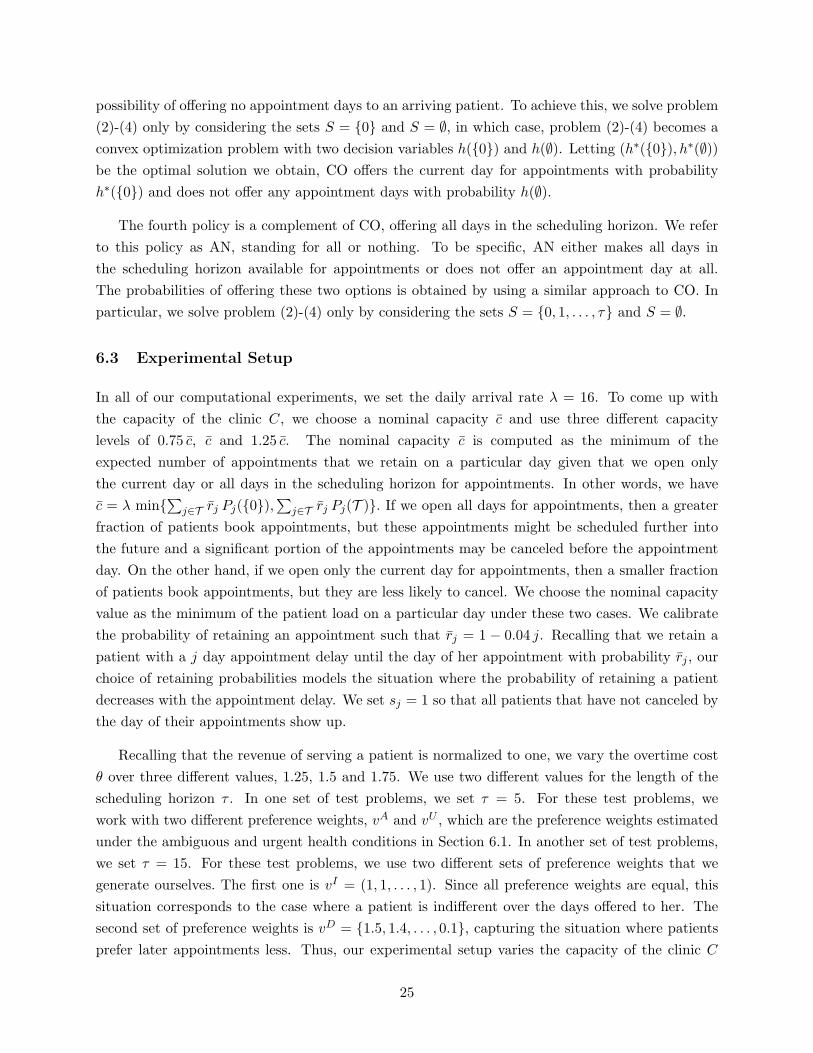
possibility of offering no appointment days to an arriving patient. To achieve this, we solve problem
(2)-(4) only by considering the sets S = {0} and S = ∅, in which case, problem (2)-(4) becomes a
convex optimization problem with two decision variables h({0}) and h(∅). Letting (h∗({0}), h∗(∅))be the optimal solution we obtain, CO offers the current day for appointments with probability
h∗({0}) and does not offer any appointment days with probability h(∅).
The fourth policy is a complement of CO, offering all days in the scheduling horizon. We refer
to this policy as AN, standing for all or nothing. To be specific, AN either makes all days in
the scheduling horizon available for appointments or does not offer an appointment day at all.
The probabilities of offering these two options is obtained by using a similar approach to CO. In
particular, we solve problem (2)-(4) only by considering the sets S = {0, 1, . . . , τ} and S = ∅.
6.3 Experimental Setup
In all of our computational experiments, we set the daily arrival rate λ = 16. To come up with
the capacity of the clinic C, we choose a nominal capacity c and use three different capacity
levels of 0.75 c, c and 1.25 c. The nominal capacity c is computed as the minimum of the
expected number of appointments that we retain on a particular day given that we open only
the current day or all days in the scheduling horizon for appointments. In other words, we have
c = λ min{∑
j∈T rj Pj({0}),∑
j∈T rj Pj(T )}. If we open all days for appointments, then a greater
fraction of patients book appointments, but these appointments might be scheduled further into
the future and a significant portion of the appointments may be canceled before the appointment
day. On the other hand, if we open only the current day for appointments, then a smaller fraction
of patients book appointments, but they are less likely to cancel. We choose the nominal capacity
value as the minimum of the patient load on a particular day under these two cases. We calibrate
the probability of retaining an appointment such that rj = 1 − 0.04 j. Recalling that we retain a
patient with a j day appointment delay until the day of her appointment with probability rj , our
choice of retaining probabilities models the situation where the probability of retaining a patient
decreases with the appointment delay. We set sj = 1 so that all patients that have not canceled by
the day of their appointments show up.
Recalling that the revenue of serving a patient is normalized to one, we vary the overtime cost
θ over three different values, 1.25, 1.5 and 1.75. We use two different values for the length of the
scheduling horizon τ . In one set of test problems, we set τ = 5. For these test problems, we
work with two different preference weights, vA and vU , which are the preference weights estimated
under the ambiguous and urgent health conditions in Section 6.1. In another set of test problems,
we set τ = 15. For these test problems, we use two different sets of preference weights that we
generate ourselves. The first one is vI = (1, 1, . . . , 1). Since all preference weights are equal, this
situation corresponds to the case where a patient is indifferent over the days offered to her. The
second set of preference weights is vD = {1.5, 1.4, . . . , 0.1}, capturing the situation where patients
prefer later appointments less. Thus, our experimental setup varies the capacity of the clinic C
25

over {0.75 c, c, 1.25c} , the overtime cost θ over {1.25, 1.5, 1.75} and the preference weights v over
{vA, vU , vI , vD}, in which case, we obtain a total of 36 test problems.
We use a simulation study to test the performance of the four policies described in the previous
section. On each day, we sample the number of appointment requests that arrive. Letting
h = {h(S) : S ⊂ T } be the probability with which each subset of days is offered to a patient
under the policy in consideration, each appointment request is offered the subset S of days with
probability h(S), independent of the others. The patient making the appointment request chooses
among the offered days according to the multinomial logit model or leaves without booking an
appointment. Once we collect the booked appointments on the current day in this fashion and
update the appointment schedule, we sample the cancellations and no shows. Based on the no-
shows, we account for the revenue and the overtime cost on the current day, after which, we can
move on to the next day. We simulate each one of the four policies for 135 days and for 100
replications. The first 45 days of each replication is used as a warm up period, during which we do
not collect any revenue or cost information.
6.4 Computational Results
Our computational results are given in Tables 1 and 2. Table 1 focuses on the test problems
with τ = 15, having the preference weights vI or vD. Table 2 focuses on the test problems with
τ = 5, having the preference weights vA or vU . The first three columns in these tables show the
characteristics of the test problems by using the triplet (v, C, θ). The following four columns show
the expected profit per day obtained by the four policies. The last three columns show the percent
gap between the expected profit per day obtained by DP and the remaining three policies.
Our results in Table 1 indicate that DP can provide substantial improvements over the other
three policies that do not consider the state of the appointment schedule when making their
decisions. For the test problems with v = vI , DP performs better than SP, CO and AN respectively
by 8.96%, 12.59% and 16.64% on average. The corresponding gaps are 6.68%, 9.92% and 13.27%
for the test problems with v = vD. In all of the test problems in Table 1, there is a statistically
significant gap between the performance of DP and the performance of the best of the remaining
three policies. Overall, the performance gaps between DP and the other three policies tend to
increase as the overtime cost gets larger. For the test problems with θ = 1.75, the performance gap
between DP and all other three policies can exceed 10%. Indeed, when the overtime cost is high,
it becomes more important to make the scheduling decisions more carefully and the improvement
provided by DP over the static policies, SP, CO and AN, become more noticeable. Interestingly, the
test problems with C = 1.25 c have relatively ample capacity, but this does not necessarily mean
that simpler static policies provide satisfactory performance.
The improvement provided by DP over the other policies can be due to both the increased
number of patients served and the decreased overtime cost. In particular, consider a policy such as
26
Prob. Char. Exp. Prof. Per Day % Gap with DPv C θ SP DP CO AN SP CO AN
vI 0.75c 1.25 5.06 5.40 5.04 4.85 6.30 6.67 10.19vI 0.75c 1.5 4.60 5.11 4.61 3.72 9.98 9.78 27.20vI 0.75c 1.75 4.32 4.87 4.30 2.69 11.29 11.70 44.76
vI c 1.25 6.93 7.36 6.52 6.93 5.84 11.41 5.84vI c 1.5 6.40 7.09 6.25 6.26 9.73 11.85 11.71vI c 1.75 6.06 6.81 6.02 5.61 11.01 11.60 17.62
vI 1.25c 1.25 7.81 8.27 6.85 7.66 5.56 17.17 7.38vI 1.25c 1.5 7.27 8.04 6.66 7.16 9.58 17.16 10.95vI 1.25c 1.75 6.89 7.77 6.53 6.67 11.33 15.96 14.16
Average 8.96 12.59 16.64
vD 0.75c 1.25 6.02 6.31 5.99 5.75 4.60 5.07 8.87vD 0.75c 1.5 5.49 5.93 5.5 4.62 7.42 7.25 22.09vD 0.75c 1.75 5.15 5.60 5.16 3.49 8.04 7.86 37.68
vD c 1.25 7.86 8.27 7.57 7.87 4.96 8.46 4.84vD c 1.5 7.31 7.91 7.26 7.16 7.59 8.22 9.48vD c 1.75 6.96 7.61 6.92 6.47 8.54 9.07 14.98
vD 1.25c 1.25 9.68 10.18 8.53 9.50 4.91 16.21 6.68vD 1.25c 1.5 9.14 9.62 8.36 9.09 4.99 13.10 5.51vD 1.25c 1.75 8.73 9.60 8.25 8.71 9.06 14.06 9.27
Average 6.68 9.92 13.27
Table 1: Performance of the four policies on the test problems with v = vI or v = vD.
AN, which does not impose a control on the days offered and either offers all days in the scheduling
horizon or does not offer anything. Due to the wide availability of options, the patients may be
more likely to book appointments under AN, but since AN offers all days, patients have the option
of booking appointments further into the future. Noting that the cancellation probabilities are
dependent on the appointment delay, more patients cancel. As a result, a policy like AN, may end
up serving a smaller number of patients when compared to DP, despite the fact that AN makes a
wide range of days available for appointments. SP alleviates this shortcoming of AN to a certain
extent since it chooses the sets of days to offer by balancing the tendency of the patients to book and
cancel appointments. On the other hand, from the perspective of overtime cost, due to their static
nature, policies such as SP, CO and AN cannot immediately react to capacities being filled up and
may schedule unnecessary overtime. Overall, DP chooses the set of days to offer by considering
the fact that a large set of days increases the likelihood that a patient books an appointment,
but appointments further into the future are more likely to be canceled. Furthermore, DP adjusts
the set of offered days in response to the current appointment schedule. Thus, DP can effectively
increase the number of patients served, while decreasing the overtime cost.
Table 2 gives our computational results for the case where the preference weights are based on
our discrete choice experiment. We observe that DP continues to provide noticeable improvements
over the other three static policies. Over the test problems with the ambiguous health condition, DP
improves the performance of SP, CO and AN respectively by 3.04%, 4.84% and 5.41% on average.
The same performance gaps come out to be 4.12%, 8.13% and 9.09% for the test problems with
27

Prob. Char. Exp. Prof. Per Day % Gap with DPv C θ SP DP CO AN SP CO AN
vA 0.75c 1.25 8.82 8.83 8.82 8.75 0.11 0.11 0.91vA 0.75c 1.5 8.22 8.25 8.23 7.78 0.36 0.24 5.70vA 0.75c 1.75 7.80 7.80 7.81 6.80 0.00 -0.13 12.82
vA c 1.25 11.42 ×11.86 11.15 11.41 3.71 5.99 3.79vA c 1.5 10.95 ×11.31 10.79 10.94 3.18 4.60 3.27vA c 1.75 10.53 10.52 10.47 10.51 -0.10 0.48 0.10
vA 1.25c 1.25 12.95 ×13.92 12.34 12.84 6.97 11.35 7.76vA 1.25c 1.5 12.80 ×13.72 12.22 12.73 6.71 10.93 7.22vA 1.25c 1.75 12.62 ×13.48 12.10 12.52 6.38 10.24 7.12
Average 3.04 4.87 5.41
vU 0.75c 1.25 6.92 6.93 6.93 6.71 0.14 0.00 3.17vU 0.75c 1.5 6.41 × 6.65 6.38 5.52 3.61 4.06 16.99vU 0.75c 1.75 6.04 × 6.30 6.05 4.37 4.13 3.97 30.63
vU c 1.25 9.70 ×10.01 9.21 9.70 3.10 7.99 3.10vU c 1.5 9.13 × 9.34 8.93 9.12 2.25 4.39 2.36vU c 1.75 8.70 8.69 8.65 8.55 -0.12 0.46 1.61
vU 1.25c 1.25 11.52 ×12.71 10.23 11.53 9.36 19.51 9.28vU 1.25c 1.5 11.36 ×12.31 10.16 11.34 7.72 17.47 7.88vU 1.25c 1.75 11.09 ×11.91 10.08 11.10 6.88 15.37 6.80
Average 4.12 8.13 9.09
Table 2: Performance of the four policies on the test problems with v = vA or v = vU .
the urgent health condition. SP provides noticeably better than CO and AN, indicating that it is
worthwhile to solve a mathematical program to find the best probability with which each subset of
days should be offered. The gap between SP and DP can still be significant and a policy, such as
DP, that makes its decisions by considering the current appointment schedule can be attractive. In
Table 2, we use a “×” to mark the test problems where the performance gap between DP and the
best performing static policy is statistically significant at 5% level. In 13 out of 18 test problems,
the performance gap is statistically significant.
Our computational experiments indicate that there are significant benefits from using dynamic
policies that explicitly consider the state of the appointment schedule. Inevitably, there is additional
computational burden brought out by dynamic policies, but for the test problems we considered,
the decision made by DP can be computed in less than 0.01 seconds. Considering that the subset
offer probabilities used by DP are recomputed at the beginning of each day, such run times are
reasonable. Furthermore, run times that are on the order of a few milliseconds are suitable even if
we recompute the subset offer probabilities for each individual patient. Online scheduling systems,
which are becoming more prevalent in practice, offer immediate access to current appointment
schedules and provide a particularly suitable environment for implementing dynamic policies.
28
7 Conclusion
Efficient use of healthcare resources is an important challenge. There is high demand for limited
resources and the demand is expected to increase in the near future, particularly in the United
States with the recent passage of the Patient Protection and Affordable Care Act. Appointment
scheduling is one way of smoothing out the variable daily patient demand, which not only helps in
increasing the utilization of resources, but also provides the patients with the flexibility of choosing
when they will be seen. Although there is a growing body of work on various aspects of appointment
scheduling, with few exceptions, the fact that patients have their own preferences regarding when
they would like to be seen has been assumed away. This paper is directed to fill this gap.
The models we propose incorporate no-shows and cancellations that are dependent on the
appointment delays, embed customer preferences among the different appointment days and take
the current appointment schedule into consideration when making decisions. We provide a number
of analytical characterizations that help simplify the way both the static and dynamic models are
solved. We give a bound on the performance of the static model. Given that the dynamic model
is obtained by applying the policy iteration algorithm on the static model, the dynamic model
is trivially guaranteed to improve the performance of the static one. Our computational results,
which make use of the patient utility estimates obtained from actual clinic data, reveal that our
dynamic model can significantly outperform other benchmark policies.
In this paper, we use the multinomial logit model to capture patient preferences. Multinomial
logit model has found many applications in economics, decision analysis and operations research to
model choice behavior and there are well-established methods for estimating the parameters of this
choice model from data. Recently, Gallego et al. (2011) describe an extension of the multinomial
logit model where the preference weight of not booking an appointment increases if too few days
are offered to patients. Under their choice model, each day in the scheduling horizon has two
parameters, denoted by vj and wj . If we offer the subset S of days, then a patient chooses day j in
the scheduling horizon with probability Pj(S) = vj/(1 +∑
k ∈S wk +∑
k∈S vk), where the quantity∑k ∈S wk captures the increase in the preference weight of not booking an appointment as a function
of the days that are not offered. It is possible to check that all of our results in the paper continue
to hold under this more general form of the multinomial logit model.
Our approach implicitly assumes that the choice behavior represented by the multinomial logit
model captures the overall patient population preferences. This approach is reasonable when we do
not have access to additional information about patient conditions. When additional information is
available, subset offer decisions may depend on the condition of patients. For example, considering
our computational study, if patients having urgent and ambiguous conditions arrive simultaneously
into the system and we have information about the condition of the patient before offering the
available appointment days, then we can define two sets of decision variables hU = {hU (S) : S ⊂ T }and hA = {hA{S) : S ⊂ T } to respectively capture the probability that each subset of days is
29
offered to a patient with urgent and ambiguous conditions. Our approach can be extended to
jointly optimize the subset offer probabilities (hU , hA).
There are a number of research directions to pursue further. First, although the multinomial
logit model is a widely used way of modeling choice, it is of interest to generalize our results to
other choice models that can capture a variety of patient preferences. The key is to keep the
corresponding optimization problems tractable, while using more intricate choice models. Second,
the current paper focuses on the aggregate capacity on each day and charges the overtime cost
by comparing the available daily capacity with the total number of appointments retained on the
current day. If the patients are scheduled for different times of the day, then it might be possible
to shift appointments within a day and still avoid overtime costs. Such an extension may result
in more intricate overtime costs as it requires keeping track of the detailed appointment dynamics
within a day and it is certainly worth investigation.
References
Ayvaz, N. and Huh, W. (2010), ‘Allocation of hospital capacity to multiple types of patients’,Journal of Revenue & Pricing Management 9(5), 386–398.
Bean, A. G. and Talaga, J. (1995), ‘Predicting appointment breaking.’, Journal of Health CareMarketing 15(1), 29–34.
Berwick, D., Nolan, T. and Whittington, J. (2008), ‘The triple aim: Care, health, and cost’, HealthAffairs 27(3), 759–769.
Bowser, D., Utz, S., Glick, D. and Harmon, R. (2010), ‘A systematic review of the relationship ofdiabetes mellitus, depression, and missed appointments in a low-income uninsured population’,Archives of psychiatric nursing 24(5), 317–329.
Bront, J. J. M., Diaz, I. M. and Vulcano, G. (2009), ‘A column generation algorithm for choice-basednetwork revenue management’, Operations Research 57(3), 769–784.
Cayirli, T. and Veral, E. (2003), ‘Outpatient scheduling in health care: A review of literature’,Production and Operations Management 12(4), 519–549.
Cayirli, T., Yang, K. K. and Quek, S. A. (2012), ‘A universal appointment rule in the presence ofno-shows and walk-ins’, Production and Operations Management . Forthcoming.
Cheraghi-Sohi, S., Hole, A., Mead, N., McDonald, R., Whalley, D., Bower, P. and Roland, M.(2008), ‘What patients want from primary care consultations: A discrete choice experiment toidentify patients priorities’, The Annals of Family Medicine 6(2), 107–115.
Denton, B. and Gupta, D. (2003), ‘A sequential bounding approach for optimal appointmentscheduling’, IIE Transactions 35(11), 1003–1016.
Dreiher, J., Froimovici, M., Bibi, Y., Vardy, D., Cicurel, A. and Cohen, A. (2008), ‘Nonattendancein obstetrics and gynecology patients’, Gynecologic and Obstetric Investigation 66(1), 40–43.
Gallego, G., Iyengar, G., Phillips, R. and Dubey, A. (2004), Managing flexible products on anetwork, Computational Optimization Research Center Technical Report TR-2004-01, ColumbiaUniversity.
30
Gallego, G., Ratliff, R. and Shebalov, S. (2011), A general attraction model and an efficientformulation for the network revenue management problem, Technical report, ColumbiaUniversity, New York, NY.
Gallego, G. and van Ryzin, G. (1994), ‘Optimal dynamic pricing of inventories with stochasticdemand over finite horizons’, Management Science 40(8), 999–1020.
Gallego, G. and van Ryzin, G. (1997), ‘A multiproduct dynamic pricing problem and its applicationsto yield management’, Operations Research 45(1), 24–41.
Gallucci, G., Swartz, W. and Hackerman, F. (2005), ‘Brief reports: Impact of the wait for an initialappointment on the rate of kept appointments at a mental health center’, Psychiatric Services56(3), 344–346.
Gerard, K., Salisbury, C., Street, D., Pope, C. and Baxter, H. (2008), ‘Is fast access to generalpractice all that should matter? A discrete choice experiment of patients’ preferences’, Journalof Health Services Research & Policy 13(suppl 2), 3–10.
Gerchak, Y., Gupta, D. and Henig, M. (1996), ‘Reservation planning for elective surgery underuncertain demand for emergency surgery’, Management Sci. 42(3), 321–334.
Green, J., McDowall, Z. and Potts, H. (2008), ‘Does choose & book fail to deliver the expectedchoice to patients? a survey of patients’ experience of outpatient appointment booking’, BMCMedical Informatics and Decision Making 8(1), 36.
Green, L., Savin, S. and Wang, B. (2006), ‘Managing patient service in a diagnostic medical facility’,Operations Research pp. 11–25.
Green, L. V. and Savin, S. (2008), ‘Reducing delays for medical appointments: A queueingapproach’, Operations Research 56(6), 1526–1538.
Grunebaum, M., Luber, P., Callahan, M., Leon, A., Olfson, M. and Portera, L. (1996), ‘Predictorsof missed appointments for psychiatric consultations in a primary care clinic’, Psychiatric Services47(8), 848–852.
Gupta, D. and Denton, B. (2008), ‘Appointment scheduling in health care: Challenges andopportunities’, IIE Transactions 40(9), 800–819.
Gupta, D. and Wang, L. (2008), ‘Revenue management for a primary-care clinic in the presence ofpatient choice’, Operations Research 56(3), 576–592.
Gupta, D. and Wang, W. (2011), Patient appointments in ambulatory care, in R. W. Hall, ed.,‘Handbook of Healthcare System Scheduling: Delivering Care When and Where It is Needed’,Springer, New York.
Hassin, R. and Mendel, S. (2008), ‘Scheduling arrivals to queues: A single-server model with no-shows’, Management Science 54(3), 565–572.
Hole, A. (2008), ‘Modelling heterogeneity in patients’ preferences for the attributes of a generalpractitioner appointment’, Journal of Health Economics 27(4), 1078–1094.
Huang, Y. and Zuniga, P. (2012), ‘Dynamic overbooking scheduling system to improve patientaccess’, Journal of the Operational Research Society . Forthcoming.
Huh, T., Liu, N. and Truong, V. (2012), ‘Multi-resource allocation scheduling in dynamicenvironments.’. Working paper. Sauder School of Busniess, University of British Columbia.
Institute for Healthcare Improvement (2012), ‘The IHI triple aim.’. Retrieved May 8, 2012, fromhttp://www.ihi.org/offerings/Initiatives/TripleAim/Pages/default.aspx.
31
Jouini, O. and Benjaafar, S. (2010), ‘Queueing systems with appointment-driven arrivals, non-punctual customers, and no-shows.’. Technical Report. University of Minnesota, Minneapolis,MN.
Kaandorp, G. C. and Koole, G. (2007), ‘Optimal outpatient appointment scheduling’, Health CareManagement Science 10(3), 217–229.
Kim, S. and Giachetti, R. E. (2006), ‘A stochastic mathematical appointment overbooking model forhealthcare providers to improve profits’, IEEE Transactions on Systems, Man and Cybernetics,Part A 36(6), 1211–1219.
Klassen, K. J. and Rohleder, T. R. (2004), ‘Outpatient appointment scheduling with urgent clientsin a dynamic, multi-period environment’, International Journal of Service Industry Management15(2), 167–186.
Kok, A., Fisher, M. and Vaidyanathan, R. (2009), ‘Assortment planning: Review of literature andindustry practice’, Retail supply chain management pp. 1–55.
Kopach, R., DeLaurentis, P. C., Lawley, M., Muthuraman, K., Ozsen, L., Rardin, R., Wan, H.,Intrevado, P., Qu, X. and Willis, D. (2007), ‘Effects of clinical characteristics on successful openaccess scheduling’, Health Care Management Science 10(2), 111–124.
Kunnumkal, S. and Topaloglu, H. (2008), ‘A refined deterministic linear program for the networkrevenue management problem with customer choice behavior’, Naval Research Logistics Quarterly55(6), 563–580.
LaGanga, L. and Lawrence, S. R. (2012), ‘Appointment overbooking in health care clinics toimprove patient service and clinic performance’, Production and Operations Management .Forthcoming.
LaGanga, L. R. and Lawrence, S. R. (2007), ‘Clinic overbooking to improve patient access andincrease provider productivity’, Decision Sciences 38(2), 251–276.
Levi, R. and Radovanovic, A. (2010), ‘Provably near-optimal LP-based policies for revenuemanagement in systems with reusable resources’, Operations Research 58(2), 503–507.
Liu, N., Ziya, S. and Kulkarni, V. G. (2010), ‘Dynamic scheduling of outpatient appointmentsunder patient no-shows and cancellations’, Manufacturing & Service Operations Management12(2), 347–364.
Liu, Q. and van Ryzin, G. (2008), ‘On the choice-based linear programming model for networkrevenue management’, Manufacturing & Service Operations Management 10(2), 288–310.
Luo, J., Kulkarni, V. G. and Ziya, S. (2012), ‘Appointment scheduling under patient no-shows andservice interruptions’, Manufacturing and Service Operations Management . Forthcoming.
McFadden, D. (1974), Conditional logit analysis of qualitative choice behavior, in P. Zarembka,ed., ‘Frontiers in Economics’, Academic Press, pp. 105–142.
Murray, M. and Tantau, C. (2000), ‘Same-day appointments: Exploding the access paradigm.’.Family Practice Management . September, 2000.
Muthuraman, K. and Lawley, M. (2008), ‘A stochastic overbooking model for outpatient clinicalscheduling with no-shows’, IIE Transactions 40(9), 820–837.
Patrick, J., Puterman, M. L. and Queyranne, M. (2008), ‘Dynamic multi-priority patient schedulingfor a diagnostic resource’, Operations Research 56(6), 1507–1525.
Qu, X., Rardin, R. L., Williams, J. A. S. and Willis, D. R. (2007), ‘Matching daily healthcareprovider capacity to demand in advanced access scheduling systems’, European Journal ofOperational Research 183(2), 812–826.
32
Rau, J. (2011), ‘Medicare to begin basing hospital payments on patient-satisfaction scores’, KaiserHealth News . Retrieved on Jan 19, 2012,http://www.kaiserhealthnews.org/Stories/2011/April/28/medicare-hospital-patient-satisfaction.aspx.
Robinson, L. W. and Chen, R. R. (2003), ‘Scheduling doctors’ appointments: Optimal andempirically-based heuristic policies’, IIE Transactions 35(3), 295–307.
Robinson, L. W. and Chen, R. R. (2010), ‘A comparison of traditional and open-access policies forappointment scheduling’, Manufacturing & Service Operations Management 12(2), 330–346.
Rohleder, T. and Klassen, K. (2000), ‘Using client-variance information to improve dynamicappointment scheduling performance’, Omega 28(3), 293–302.
Rubin, G., Bate, A., George, A., Shackley, P. and Hall, N. (2006), ‘Preferences for access to theGP: A discrete choice experiment’, The British Journal of General Practice 56(531), 743.
Rusmevichientong, P., Shmoys, D. B. and Topaloglu, H. (2010), Assortment optimization withmixtures of logits, Technical report, Cornell University, School of Operations Research andInformation Engineering.Available at http://people.orie.cornell.edu/huseyin/publications/publications.html.
Ruszczynski, A. (2006), Nonlinear Optimization, Princeton University Press, Princeton, NewJersey.
Ryan, M. and Farrar, S. (2000), ‘Using conjoint analysis to elicit preferences for health care’, Bmj320(7248), 1530.
Sampson, F., Pickin, M., O’Cathain, A., Goodall, S. and Salisbury, C. (2008), ‘Impact of same-dayappointments on patient satisfaction with general practice appointment systems’, The BritishJournal of General Practice 58(554), 641–643.
Schectman, J., Schorling, J. and Voss, J. (2008), ‘Appointment adherence and disparities inoutcomes among patients with diabetes’, Journal of general internal medicine 23(10), 1685–1687.
Silvestre, A., Sue, V. M. and Allen, J. Y. (2009), ‘If you build it, will they come? the kaiserpermanente model of online health care’, Electronic Health Records 28, 334–344.
Talluri, K. and van Ryzin, G. (2004a), ‘Revenue management under a general discrete choice modelof consumer behavior’, Management Science 50(1), 15–33.
Talluri, K. and Van Ryzin, G. (2004b), ‘Revenue management under a general discrete choice modelof consumer behavior’, Management Science pp. 15–33.
Topaloglu, H. (2010), Joint stocking and product offer decisions under the multinomial logitmodel, Technical report, Cornell University, School of Operations Research and InformationEngineering.Available at http://people.orie.cornell.edu/huseyin/publications/publications.html.
Topaloglu, H., Birbil, S., Frenk, J. and Noyan, N. (2011), ‘Tractable open loop policies for jointoverbooking and capacity control over a single flight leg with multiple fare classes’, TransportationScience (to appear).
US Department of Health and Human Services (2011), ‘Electronic health records and meaningfuluse’. Retrieved on Jan 19, 2012, http://healthit.hhs.gov/.
Wang, P. (1999), ‘Sequencing and scheduling N customers for a stochastic server’, European journalof operational research 119(3), 729–738.
33

Wang, W. and Gupta, D. (2011), ‘Adaptive appointment systems with patient preferences’,Manufacturing & Service Operations Management 13(3), 373–389.
Weiner, M., El Hoyek, G., Wang, L., Dexter, P. R., Zerr, A. D., Perkins, A. J., James, F. andJuneja, R. (2009), ‘A web-based generalist-specialist system to improve scheduling of outpatientspecialty consultations in an academic center’, Journal of General Internal Medicine 6, 710–715.
Zeng, B., Turkcan, A., Lin, J. and Lawley, M. (2010), ‘Clinic scheduling models with overbooking forpatients with heterogeneous no-show probabilities.’, Annals of Operations Research 178(1), 121–144.
Zhang, D. and Adelman, D. (2009), ‘An approximate dynamic programming approach to networkrevenue management with customer choice’, Transportation Science 42(3), 381–394.
Zocdoc (2012), ‘About us.’. Retrieved on Jan 19, 2012, http://www.zocdoc.com/aboutus.
34

A Appendix: Omitted Results
In this section, we give the proofs of the results that are omitted in the paper.
A.1 Proof of Proposition 1
We complete the proof of Proposition 1 in two parts. First, assume that h∗ = {h∗(S) : S ⊂ T } is an
optimal solution to problem (2)-(4). Letting x∗j =∑
S⊂T Pj(S)h∗(S) and u∗ =
∑S⊂T N(S)h∗(S),
we need to show that (x∗, u∗) is a feasible solution to problem (5)-(8) providing the same objective
value as the solution h∗. We have∑j∈T
x∗j + u∗ =∑S⊂T
h∗(S)[∑j∈T
Pj(S) +N(S)] =∑S⊂T
h∗(S) = 1,
where the second equality follows by the definition of the multinomial logit model and the third
equality follows since h∗ is feasible to problem (2)-(4). Thus, the solution (x∗, u∗) satisfies the first
constraint in problem (5)-(8). On the other hand, using 1(·) to denote the indicator function, we
have x∗j/vj =∑
S⊂T [1(j ∈ S)h∗(S)/(1 +∑
k∈S vk)] by the definition of Pj(S) in the multinomial
logit model. Noting that u =∑
S⊂T [h∗(S)/(1 +
∑k∈S vk)], it follows that x∗j/vj ≤ u, indicating
that the solution (x∗, u∗) satisfies the second set of constraints in problem (5)-(8). Since x∗j =∑S⊂T Pj(S)h
∗(S), comparing the objective functions of problems (2)-(4) and (5)-(8) shows that
the solutions h∗ and (x∗, u∗) provide the same objective values for their problems.
Second, assume that (x∗, u∗) is a feasible solution to problem (5)-(8). We construct the solution
h∗ as in (9). To see that the solutions (x∗, u∗) and h∗ provide the same objective values for their
respective problems, we observe that
∑S⊂T
Pj(S)h∗(S) =
τ∑i=0
Pj(Si)h∗(Si) =
τ∑i=j
Pj(Si)h∗(Si) =
τ∑i=j
vj
[x∗ivi
−x∗i+1
vi+1
]= x∗j ,
where the first equality is by the fact that h∗(S) takes positive values only for the sets S0, . . . , Sτ
and ∅, the second equality is by the fact that j ∈ Si only when j ≤ i and the third equality follows
by the definition of h∗(Si) and noting that x∗τ+1 = 0. Using the equality above and comparing the
objective functions of problems (2)-(4) and (5)-(8) show that the solutions h∗ and (x∗, u∗) provide
the same objective values for their problems. To see that the solution h∗ is feasible to problem
(2)-(4), we let Vi = 1 +∑
k∈Sivk for notational brevity and write
∑S⊂T h∗(S) as
u∗ − x∗0v0
+
τ∑j=0
Vj
[x∗jvj
−x∗j+1
vj+1
]= u∗ + (V0 − 1)
x∗0v0
+ (V1 − V0)x∗1v1
+ . . .+ (Vτ − Vτ−1)x∗τvτ
= 1,
where the first equality follows by rearranging the terms and using the convention that x∗τ+1 = 0
and the second equality is by noting that Vi − Vi−1 = vi and using the fact that (x∗, u∗) is feasible
to problem (5)-(8) so that∑τ
j=0 x∗j + u∗ = 1. 2
35

A.2 Proof of Proposition 6
The proof follows from an argument similar to the one in the proof of Proposition 1. Assume that
h∗ = {h∗(S) : S ⊂ T } is an optimal solution to problem (2)-(4) with the additional constraints
ht(S) ∈ {0, 1} for all S ⊂ T . Letting x∗j =∑
S⊂T Pj(S)h∗(S) and u∗ =
∑S⊂T N(S)h∗(S), we can
follow the same argument in Section A.1 to show that (x∗, u∗) with x∗ = (x∗0, . . . , x∗τ ) is a feasible
solution to problem (5)-(8) with the additional constraints xj/vj ∈ {0, u} for all j ∈ T . Furthermore,
the objective values provided by the two solutions for their respective problems are identical. On
the other hand, assume that (x∗, u∗) with x∗ = (x∗0, . . . , x∗τ ) is an optimal solution to problem
(5)-(8) with the additional constraints xj/vj ∈ {0, u} for all j ∈ T . We reorder and reindex the
days in the scheduling horizon so that we have u∗ = x∗0/v0 = x∗1/v∗1 = . . . = x∗j−1/v
∗j−1 ≥ x∗j/xj =
x∗j+1/vj+1 = . . . = x∗τ/v∗τ = 0. We define the subsets S0, S1, . . . , Sτ as Sj = {0, 1, . . . , j}. For
notational convenience, we define x∗τ+1 = 0. In this case, letting
h∗(∅) = u∗ − x∗0v0
and h∗(Sj) =[1 +
∑k∈Sj
vk
] [x∗jvj
−x∗j+1
vj+1
]for all j = 0, 1, . . . , τ and letting h∗(S) = 0 for all other subsets of T , we can follow the same
argument in Section A.1 to show that {h∗(S) : S ⊂ T } is a feasible solution to problem (2)-(4)
with the additional constraints ht(S) ∈ {0, 1} for all S ⊂ T . Furthermore, we can check that the
two solutions provide the same objective value for their respective problems. 2
A.3 Lemma 7
The following lemma is used in Section 4.
Lemma 7. Letting F (α) = E{[Pois(α)− C]+
}, F (·) is differentiable and convex.
Proof. The proof uses elementary properties of the Poisson distribution. By using the probability
mass function of the Poisson distribution, we have
F (α) =
∞∑i=C+1
e−α αi
i!(i− C) =
∞∑i=C+1
e−α αi
(i− 1)!−
∞∑i=C+1
e−α αi
i!C
= α
∞∑i=C
e−α αi
i!− C
∞∑i=C+1
e−α αi
i!= αP{Pois(α) ≥ C} − C P{Pois(α) ≥ C + 1}. (26)
Thus, the differentiability of F (·) follows by the differentiability of the cumulative distribution
function of the Poisson distribution with respect to its mean. For the convexity of F (·), we have
dP{Pois(α) ≥ C}dα
= −dP{Pois(α) ≤ C − 1}dα
= −C−1∑i=0
d(e−α αi
i!
)dα
=C−1∑i=0
e−α αi
i!−
C−1∑i=1
e−α αi−1
(i− 1)!= P{Pois(α) = C − 1}.
36

In this case, if we differentiate both sides of (26) with respect to α and use the last chain of
equalities, then we obtain
dF (α)
dα= P{Pois(α) ≥ C}+ αP{Pois(α) = C − 1} − C P{Pois(α) = C}
= P{Pois(α) ≥ C}+ αe−α αC−1
(C − 1)!− C
e−α αC
C!= P{Pois(α) ≥ C}.
To see that F (·) is convex, we use the last two chains of equalities to observe that the second
derivative of F (α) with respect to α is P{Pois(α) = C − 1
}, which is positive. 2
A.4 Proof of Lemma 4
We let π∗(S) be the steady state probability with which we offer the subset S of days under the
optimal, possibly state-dependent, policy. So, if we consider a particular day in steady state, then
the number of patients that are scheduled for this day j days in advance is given by a Poisson random
variable with mean∑
S⊂T λPj(S)π∗(S). Therefore, if we use the random variable A∗
j to denote
the number of patients that we schedule for a particular day j days in advance in steady state, then
A∗j has mean
∑S⊂T λPj(S)π
∗(S). We note that A∗1, A
∗2, . . . , A
∗τ are not necessarily independent of
each other, since the decisions under the optimal state-dependent policy on different days can be
dependent. Similarly, in steady state, we let S∗j be the number of patients that we schedule for a
particular day j days in advance and that show up under the optimal state-dependent policy. Finally,
we let R∗j be the number of patients that we schedule for a particular day j days in advance and that
we retain until the morning of the appointment under the optimal state dependent policy. Noting
that the show-up and cancellation decisions of the patients are independent of how many patients
we schedule for a particular day, we have E{S∗j } = sj E{A∗
j} and E{R∗j} = rj E{A∗
j}. In this case,
the average profit per day generated by the optimal state-dependent policy satisfies
V ∗ = E{∑
j∈TS∗j
}− θE
{[∑j∈T
R∗j − C
]+}≤
∑j∈T
E{S∗j } − θ
[∑j∈T
E{R∗j} − C
]+=
∑j∈T
∑S⊂T
λ sj Pj(S)π∗(S)− θ
[∑j∈T
∑S⊂T
λ rj Pj(S)π∗(S)− C
]+≤ ZDET .
In the chain of inequalities above, the first inequality is by the Jensen’s inequality. The second
equality is by E{S∗j } = sj E{A∗
j} and E{R∗j} = rj E{A∗
j}. To see the second inequality, we note
that {π∗(S) : S ⊂ T } is a feasible but not necessarily an optimal solution to the problem
max∑j∈T
∑S⊂T
λ sj Pj(S)w(S)− θ[∑j∈T
∑S⊂T
λ rj Pj(S)w(S)− C]+
subject to∑S⊂T
w(S) = 1
w(S) ≥ 0 S ⊂ T
and the optimal objective values of the problem above and problem (20)-(23) are equal to each
other, which can be verified by using the argument in the proof of Proposition 1. 2
37

A.5 Lemma 8
The following result is used in the proof of Proposition 5.
Lemma 8. It holds that E{[Pois(α)− C]+} ≤ [α− C]+ + α/√2π C.
Proof. For k ≥ C + 1, we observe that [k − C]+ − [α − C]+ ≤ k − α. In particular, for k ≥ α,
this inequality follows by the Lipschitz continuity of the function [· − C]+. For k < α, we have
C + 1 ≤ k < α and it follows [k − C]+ − [α − C]+ = k − α, establishing the desired inequality. In
this case, the result in the lemma follows by noting that
E{[Pois(α)− C]+} =
∞∑k=C+1
[k − C]+e−ααk
k!≤ [α− C]+ +
∞∑k=C+1
[[k − C]+ − [α− C]+
] e−ααk
k!
≤ [α− C]+ +
∞∑k=C+1
(k − α)e−ααk
k!= [α− C]+ +
e−ααC
C!α ≤ [α− C]+ +
e−CCC
C!α,
where the first inequality follows by adding and subtracting [α − C]+ to the expression on the
left side of this inequality, the second inequality follows by the inequality derived at the beginning
of the proof, the last equality is by arranging the terms in the summation on the left side of
this inequality and the third inequality is by noting that the function f(α) = e−ααC attains its
maximum at α = C. In this case, the result follows by noting that C! ≥√2π C(C/e)C by Stirling’s
approximation and using this bound on the right side of the chain of inequalities above. 2
38