Susan Athey

Guido W. Imbens

Stefan Wager

October, 2017

Working Paper No. 17-029

Approximate Residual Balancing: De-Biased

Inference of Average Treatment Effects in

High Dimensions

Approximate Residual Balancing: De-Biased Inference of Average

Treatment Effects in High Dimensions∗

Susan Athey† Guido W. Imbens‡ Stefan Wager§

Current version August 2017

Abstract

There are many settings where researchers are interested in estimating average treatment effectsand are willing to rely on the unconfoundedness assumption, which requires that the treatmentassignment be as good as random conditional on pre-treatment variables. The unconfoundednessassumption is often more plausible if a large number of pre-treatment variables are included in theanalysis, but this can worsen the performance of standard approaches to treatment effect estimation.In this paper, we develop a method for de-biasing penalized regression adjustments to allow sparseregression methods like the lasso to be used for

√n-consistent inference of average treatment effects

in high-dimensional linear models. Given linearity, we do not need to assume that the treatmentpropensities are estimable, or that the average treatment effect is a sparse contrast of the outcomemodel parameters. Rather, in addition standard assumptions used to make lasso regression on theoutcome model consistent under 1-norm error, we only require overlap, i.e., that the propensity scorebe uniformly bounded away from 0 and 1. Procedurally, our method combines balancing weightswith a regularized regression adjustment.

Keywords: Causal Inference, Potential Outcomes, Propensity Score, Sparse Estimation

1 Introduction

In order to identify causal effects in observational studies, practitioners may assume treatment assign-ments to be as good as random (or unconfounded) conditional on observed features of the units; seeRosenbaum and Rubin (1983) and Imbens and Rubin (2015) for general discussions. Motivated by thissetup, there is a large literature on how to adjust for differences in observed features between the treatmentand control groups; some popular methods include regression, matching, propensity score weighting andsubclassification, as well as doubly-robust combinations thereof (e.g., Abadie and Imbens, 2006; Heckmanet al., 1998; Hirano et al., 2003; Robins et al., 1994, 1995, 2017; Rosenbaum, 2002; Tan, 2010; Tsiatis,2007; Van Der Laan and Rubin, 2006).

In practice, researchers sometimes need to account for a substantial number of features to make thisassumption of unconfoundedness plausible. For example, in an observational study of the effect of fluvaccines on hospitalization, we may be concerned that only controlling for differences in the age andsex distribution between controls and treated may not be sufficient to eliminate biases. In contrast,controlling for detailed medical histories and personal characteristics may make unconfoundedness more

∗We are grateful for detailed comments from Jelena Bradic, Edgar Dobriban, Bryan Graham, Chris Hansen, NishanthMundru, Jamie Robins and Jose Zubizarreta, and for discussions with seminar participants at the Atlantic Causal Infer-ence Conference, Boston University, the Columbia Causal Inference Conference, Columbia University, Cowles Foundation,the Econometric Society Winter Meeting, the EGAP Standards Meeting, the European Meeting of Statisticians, ICML,INFORMS, Stanford University, UNC Chapel Hill, University of Southern California, and the World Statistics Congress.†Professor of Economics, Stanford Graduate School of Business, and NBER, athey@stanford.edu.‡Professor of Economics, Stanford Graduate School of Business, and NBER, imbens@stanford.edu.§Assistant Professor of Operations, Information and Technology and of Statistics (by courtesy), Stanford Graduate

School of Business, swager@stanford.edu.

1

arX

iv:1

604.

0712

5v4

[st

at.M

E]

17

Aug

201

7

plausible. But the formal asymptotic theory in the earlier literature only considers the case where thesample size increases while the number of features remains fixed, and so approximations based on thoseresults may not yield valid inferences in settings where the number of features is large, possibly evenlarger than the sample size.

There has been considerable recent interest in adapting methods from the earlier literature to high-dimensional settings. Belloni et al. (2014, 2017) show that attempting to control for high-dimensionalconfounders using a regularized regression adjustment obtained via, e.g., the lasso, can result in substan-tial biases. Belloni et al. (2014) propose an augmented variable selection scheme to avoid this effect, whileBelloni et al. (2017), Chernozhukov et al. (2017), Farrell (2015), and Van der Laan and Rose (2011) buildon the work of Robins et al. (1994, 1995) and discuss how a doubly robust approach to average treatmenteffect estimation in high dimensions can also be used to compensate for the bias of regularized regressionadjustments. Despite the breadth of research on the topic, all the above papers rely crucially on theexistence of a consistent estimator of the propensity score, i.e., the conditional probability of receivingtreatment given the features, in order to yield

√n-consistent estimates of the average treatment effect in

high dimensions.1

In this paper, we show that in settings where we are willing to entertain a sparse, well-specified linearmodel on the outcomes, efficient inference of average treatment effects in high-dimensions is possible underweaker assumptions than suggested by the literature discussed above. Given linearity assumptions, weshow that it is not necessary to consistently estimate treatment propensities; rather, it is enough to relyon de-biasing techniques building on recent developments in the high-dimensional inference literature(Javanmard and Montanari, 2014, 2015; Van de Geer et al., 2014; Zhang and Zhang, 2014). In particular,in sparse linear models, we show that

√n-consistent inference of average treatment effects is possible

provided we simply require overlap, i.e., that the propensity score be uniformly bounded away from 0and 1 for all values in the support of the pretreatment variables. We do not need to assume the existenceof a consistent estimator of the propensity scores, or any form of sparsity on the propensity model.

The starting point behind both our method and the doubly robust methods of Belloni et al. (2017),Chernozhukov et al. (2017), Farrell (2015), Van der Laan and Rose (2011), etc., is a recognition that highdimensional regression adjustments (such as the lasso) always shrink estimated effects, and that ignoringthis shrinkage may result in prohibitively biased treatment effect estimates. The papers on doublyrobust estimation then proceed to show that propensity-based adjustments can be used to compensatefor this bias, provided we have a consistent propensity model that converges fast enough to the truth.Conceptually, this work builds on the result of Rosenbaum and Rubin (1983), who showed that controllingfor the propensity score is sufficient to remove all biases associated with observed covariates, regardlessof their functional form.

If we are willing to focus on high-dimensional linear models, however, it is possible to tighten theconnection between the estimation strategy and the objective of estimating the average treatment effectand, in doing so, extend the number of settings where

√n-consistent inference is possible. The key insight

is that, in a linear model, propensity-based methods are attempting to solve a needlessly difficult taskwhen they seek to eliminate biases of any functional form. Rather, in linear models, it is enough tocorrect for linear biases. In high dimensions, this can still be challenging; however, we find that it ispossible to approximately correct for such biases whenever we assume overlap.

Concretely, we study the following two stage approximate residual balancing algorithm. First, we fita regularized linear model for the outcome given the features separately in the two treatment groups. Inthe current paper we focus on the elastic net (Zou and Hastie, 2005) and the lasso (Chen et al., 1998;Tibshirani, 1996) for this component, and present formal results for the latter. In a second stage, were-weight the first stage residuals using weights that approximately balance all the features between thetreatment and control groups. Here we follow Zubizarreta (2015), and optimize the implied balance andvariance provided by the weights, rather than the fit of the propensity score. Approximate balancingon all pretreatment variables (rather than exact balance on a subset of features, as in a regularizedregression, or weighting using a regularized propensity model that may not be able to capture all relevant

1Some of the above methods assume that the propensity scores can be consistently estimated using a sparse logisticmodel, while others allow for the use of more flexible modeling strategies following, e.g., McCaffrey et al. (2004), Van derLaan et al. (2007), or Westreich et al. (2010).

2

dimensions) allows us to guarantee that the bias arising from a potential failure to adjust for a largenumber of weak confounders can be bounded. Formally, this second step of re-weighting residuals usingthe weights proposed by Zubizarreta (2015) is closely related to de-biasing corrections studied in thehigh-dimensional regression literature (Javanmard and Montanari, 2014, 2015; Van de Geer et al., 2014;Zhang and Zhang, 2014); we comment further on this connection in Section 3.

This approach also bears a close conceptual connection to work by Chan et al. (2015), Deville andSarndal (1992), Graham et al. (2012, 2016), Hainmueller (2012), Hellerstein and Imbens (1999), Imai andRatkovic (2014) and Zhao (2016), who effectively fit propensity models to the data under a constraintthat the resulting inverse-propensity weights exactly balance the covariate distributions between thetreatment and control groups, and find that these methods out-perform propensity-based methods thatdo not impose balance. Such methods, however, are of course only possible in low dimensions; in highdimensions where there are more covariates than samples, achieving exact balance is in general impossible.One of the key findings of this paper is that, in high dimensions, it is still often possible to achieveapproximate balance under reasonable assumptions and that—when combined with a lasso regressionadjustment—approximate balance suffices for eliminating bias due to regularization.

In our simulations, we find that three features of the algorithm are important: (i) the direct covarianceadjustment based on the outcome data with regularization to deal with the large number of features,(ii) the weighting using the relation between the treatment and the features, and (iii) the fact that theweights are based on direct measures of imbalance rather than on estimates of the propensity score. Thefinding that both weighting and regression adjustment are important is similar to conclusions drawn fromthe earlier literature on doubly robust estimation (e.g., Robins and Ritov, 1997), where combining bothtechniques was shown to extend the set of problems where efficient treatment effect estimation is possible.The finding that weights designed to achieve balance perform better than weights based on the propensityscore is consistent with findings in Chan et al. (2015), Graham et al. (2012, 2016), Hainmueller (2012),Imai and Ratkovic (2014), and Zubizarreta (2015).

Our paper is structured as follows. First, in Section 2, we motivate our two-stage procedure using asimple bound for its estimation error. Then, in Section 3, we provide a formal analysis of our procedureunder high-dimensional asymptotics, and we identify conditions under which approximate residual bal-ancing is asymptotically Gaussian and allows for practical inference about the average treatment effectwith dimension-free rates of convergence. Finally, in Section 5, we conduct a simulation experiment, andfind our method to perform well in a wide variety of settings relative to other proposals in the literature.A software implementation for R is available at https://github.com/swager/balanceHD.

2 Estimating Average Treatment Effects in High Dimensions

2.1 Setting and Notation

Our goal is to estimate average treatment effects in the potential outcome framework, or Rubin CausalModel (Rubin, 1974; Imbens and Rubin, 2015). For each unit in a large population there is pair of(scalar) potential outcomes, (Yi(0), Yi(1)). Each unit is assigned to the treatment or not, with thetreatment indicator denoted by Wi ∈ 0, 1. Each unit is also characterized by a vector of covariates orfeatures Xi ∈ Rp, with p potentially large, possibly larger than the sample size. For a random sample ofsize n from this population, we observe the triple (Xi, Wi, Y

obsi ) for i = 1, . . . , n, where

Y obsi = Yi(Wi) =

Yi(1) if Wi = 0,

Yi(0) if Wi = 1,(1)

is the realized outcome, equal to the potential outcome corresponding to the actual treatment received.The total number of treated units is equal to nt and the number of control units equals nc. We frequentlyuse the short-hand Xc and Xt for the feature matrices corresponding only to control or treated unitsrespectively. We write the propensity score, i.e., the conditional probability of receiving the treatmentgiven features, as e(x) = P[Wi = 1|Xi = x] (Rosenbaum and Rubin, 1983). We focus primarily on the

3

conditional average treatment effect for the treated sample,

τ =1

nt

∑i:Wi=1

E[Yi(0)− Yi(1)

∣∣Xi

]. (2)

We note that the average treatment effect for the controls and the overall average effect can be handledsimilarly. Throughout the paper we assume unconfoundedness, i.e., that conditional on the pretreatmentvariables, treatment assignment is as good as random (Rosenbaum and Rubin, 1983); we also assume alinear model for the potential outcomes in both groups.

Assumption 1 (Unconfoundedness). Wi ⊥⊥ (Yi(0), Yi(1))∣∣ Xi.

Assumption 2 (Linearity). The conditional response functions satisfy µc(x) = E[Yi(0)

∣∣X = x]

= x ·βcand µt(x) = E

[Yi(1)

∣∣X = x]

= x · βt, for all x ∈ Rp.

Here, we will only use the linear model for the control outcome because we focus on the average effectfor the treated units, but if we were interested in the overall average effect we would need linearity in bothgroups. The linearity assumption is strong, but in high dimensions some strong structural assumption isin general needed for inference to be possible. Then, given linearity, we have

τ = µt − µc, where µt = Xt · βt, µc = Xt · βc, and Xt =1

nt

n∑i=1

1 (Wi = 1)Xi. (3)

Estimating the first term is easy: µt = Y t =∑i:Wi=1 Y

obsi /nt is unbiased for µt. In contrast, estimating

µc is a major challenge, especially in settings where p is large, and it is the main focus of the paper.

2.2 Baselines and Background

We begin by reviewing two classical approaches to estimating µc, and thus also τ , in the above linearmodel. The first is a weighting-based approach, which seeks to re-weight the control sample to make itlook more like the treatment sample; the second is a regression-based approach, which seeks to adjust fordifferences in features between treated and control units by fitting an accurate model to the outcomes.Though neither approach alone performs well in a high-dimensional setting with a generic propensityscore, we find that these two approaches can be fruitfully combined to obtain better estimators for τ .

2.2.1 Weighted Estimation

A first approach is to re-weight the control dataset using weights γi to make the weighted covariatedistribution mimic the covariate distribution in the treatment population. Given the weights we estimateµc as a weighted average µc =

∑i:Wi=0 γi Y

obsi . The standard way of selecting weights γi uses the

propensity score: γi = e(Xi)/(1− e(Xi)) / (∑i:Wj=0 e(Xj)/(1− e(Xj))). To implement these methods

researchers typically substitute an estimate of the propensity score into this expression. Such inverse-propensity weights with non-parametric propensity score estimates have desirable asymptotic propertiesin settings with a small number of covariates (Hirano et al., 2003). The finite-sample performance ofmethods based on inverse-propensity weighting can be poor, however, both in settings with limitedoverlap in covariate distributions and in settings with many covariates. A key difficulty is that estimatingthe treatment effect then involves dividing by 1− e(Xi), and so small inaccuracies in e(Xi) can have largeeffects, especially when e(x) can be close to one; this problem is often quite severe in high dimensions.

As discussed in the introduction, if the control potential outcomes Yi(0) have a linear dependence onXi, then using weights γi that explicitly seek to balance the features Xi is often advantageous (Devilleand Sarndal, 1992; Chan et al., 2015; Graham et al., 2012, 2016; Hainmueller, 2012; Hellerstein andImbens, 1999; Imai and Ratkovic, 2014; Zhao, 2016; Zubizarreta, 2015). This is a subtle but importantimprovement. The motivation behind this approach is that, in a linear model, the bias for estimatorsbased on weighted averaging depends solely on Xt −

∑i:Wi=0 γiXi. Therefore getting the propensity

4

model exactly right is less important than accurately matching the moments of Xt. In high dimensions,however, exact balancing weights do not in general exist. When p nc, there will in general be noweights γi for which Xt −

∑i:Wi=0 γiXi = 0, and even in settings where p < nc but p is large such

estimators would not have good properties. Zubizarreta (2015) extends the balancing weights approachto allow for weights that achieve approximate balance instead of exact balance; however, directly usinghis approach does not allow for

√n-consistent estimation in a regime where p is much larger than n.

2.2.2 Regression Adjustments

A second approach is to compute an estimator βc for βc using the nc control observations, and thenestimate µc as µc = Xt ·βc. In a low-dimensional regime with p nc, the ordinary least squares estimatorfor βc is a natural choice, and yields an accurate and unbiased estimate of µc. In high dimensions, however,the problem is more delicate: Accurate unbiased estimation of the regression adjustment is in generalimpossible, and methods such as the lasso, ridge regression, or the elastic net may perform poorly whenplugged in for βc, in particular when Xt is far away from Xc. As stressed by Belloni et al. (2014), theproblem with plain lasso regression adjustments is that features with a substantial difference in averagevalues between the two treatment arms can generate large biases even if the coefficients on these featuresin the outcome regression are small. Thus, a regularized regression that has been tuned to optimizegoodness of fit on the outcome model is not appropriate whenever bias in the treatment effect estimatedue to failing to control for potential confounders is of concern. To address this problem, Belloni et al.(2014) propose running least squares regression on the union of two sets of selected variables, one selectedby a lasso regressing the outcome on the covariates, and the other selected by a lasso logistic regressionfor the treatment assignment. We note that estimating µc by a regression adjustment µc = Xt · βc, withβc estimated by ordinary least squares on a selected variables, is implicitly equivalent to using a weightedaveraging estimator with weights γ chosen to balance the selected features (Robins et al., 2007). TheBelloni et al. (2014) approach works well in settings where both the outcome regression and the treatmentregression are at least approximately sparse. However, when the propensity is not sparse, we find thatthe performance of such double-selection methods is often poor.

2.3 Approximate Residual Balancing

Here we propose a new method combining weighting and regression adjustments to overcome the limita-tions of each method. In the first step of our method, we use a regularized linear model, e.g., the lassoor the elastic net, to obtain a pilot estimate of the treatment effect. In the second step, we do “approxi-mate balancing” of the regression residuals to estimate treatment effects: We weight the residuals usingweights that achieve approximate balance of the covariate distribution between treatment and controlgroups. This step compensates for the potential bias of the pilot estimator that arises due to confoundersthat may be weakly correlated with the outcome but are important due to their correlation with thetreatment assignment. We find that the regression adjustment is effective at capturing strong effects; theweighting on the other hand is effective at capturing small effects. The combination leads to an effectiveand simple-to-implement estimator for average treatment effects with many features.

We focus on a meta-algorithm that first computes an estimate βc of βc using the full sample of controlunits. This estimator may take a variety of forms, but typically it will involve some form of regularizationto deal with the number of features. Second we compute weights γi that balance the covariatees at leastapproximately, and apply these weights to the residuals (Cassel et al., 1976; Robins et al., 1994):

µc = Xt · βc +∑

i:Wi=0

γi

(Y obsi −Xi · βc

). (4)

In other words, we fit a model parametrized by βc to capture some of the strong signals, and then usea non-parametric re-balancing of the control data on the features to extract left-over signal from theresiduals Y obs

i −Xi · βc. Ideally, we would hope for the first term to take care of any strong effects, whilethe re-balancing of the residuals can efficiently take care of the small spread-out effects. Our theory andexperiments will verify that this is in fact the case.

5

A major advantage of the functional form in (4) is that it yields a simple and powerful theoreticalguarantee, as stated below. Recall that Xc is the feature matrix for the control units. Consider thedifference between µc and µc for our proposed approach: µc − µc = (Xt −X>c γ) · (βc − βc) + γ · ε, whereε is the intrinsic noise εi = Yi(0) −Xi · βc. With only the regression adjustment and no weighting, the

difference would be µc,reg−µc = (Xt−Xc) ·(βc−βc)+1 ·ε/nc, and with only the weighting the differencewould be µc,weight−µc = (Xt−X>c γ) ·βc +γ ·ε. Without any adjustment, just using the average outcomefor the controls as an estimator for µc, the difference between the estimator for µc and its actual valuewould be µc,no−adj − µc = (Xt −Xc) · βc + 1 · ε/nc. The regression reduces the bias from (Xt −Xc) · βcto (Xt − Xc) · (βc − βc), which will be substantial reduction if the estimation error (βc − βc) is small

relative to βc. The weighting further reduces this to (Xt−X>c γ) · (βc−βc), which may be helpful if thereis a substantial difference between Xt and Xc. This result, formalized below, shows the complimentarynature of the regression adjustment and the weighting. All proofs are given in the appendix.

Proposition 1. The estimator (4) satisfies |µc − µc| ≤∥∥Xt −X>c γ

∥∥∞

∥∥∥βc − βc∥∥∥1

+∣∣∣∑i:Wi=0 γi εi

∣∣∣.This result decomposes the error of µc into two parts. The first is a bias term reflecting the dimension

p of the covariates; the second term is a variance term that does not depend on it. The upshot is that thebias term, which encodes the high-dimensional nature of the problem, involves a product of two factorsthat can both other be made reasonably small; we will focus on regimes where the first term shouldbe expected to scale as O(

√log(p)/n), while the second term scales as O(k

√log(p)/n) where k is the

sparsity of the outcome model. If we are in a sparse enough regime (i.e., k is small enough), Proposition1 implies that our procedure will be variance dominated; and, under these conditions, we also show thatit is

√n-consistent.

In order to exploit Proposition 1, we need to make concrete choices for the weights γ and the parameterestimates βc. First, just like Zubizarreta (2015), we choose our weights γ to directly optimize the biasand variance terms in Proposition 1; the functional form of γ is given in (5), where ζ ∈ (0, 1) is a tuningparameter. We refer to them as approximately balancing weights since they seek to make the mean of there-weighted control sample, namely X>c γ, match the treated sample mean Xt as closely as possible. Thepositivity constraint on γi in (5) aims to prevent the method from extrapolating too aggressively, while

the upper bound is added for technical reasons discussed in Section 3. Meanwhile, for estimating βc, wesimply need to use an estimator that achieves good enough risk bounds under L1-risk. In our analysis,we focus on the lasso (Chen et al., 1998; Tibshirani, 1996); however, in experiments, we use the elasticnet for additional stability (Zou and Hastie, 2005). Our complete algorithm is described in Procedure 1.

Finally, although we do use this estimator in the present paper, we note that an analogous estimatorfor the average treatment effect E [Y (1)− Y (0)] can also be constructed:

τATE = X(βt − βc

)+

∑i:Wi=1

γt,i

(Y obsi −Xi · βt

)−

∑i:Wi=0

γc,i

(Y obsi −Xi · βc

), where

γt = argminγ

(1− ζ) ‖γ‖22 + ζ∥∥X −X>t γ

∥∥2∞ subject to

∑i:Wi=1

γi = 1 and 0 ≤ γi ≤ n−2/3t

,

(8)

and γc is constructed similarly. This method can be analyzed using the same tools developed in thispaper, and is available in our software package balanceHD.

2.4 Connection to Doubly Robust Estimation

The idea of combining weighted and regression-based approaches to treatment effect estimation has a longhistory in the causal inference literature. Given estimated propensity scores e(Xi), Cassel et al. (1976)and Robins et al. (1994) propose using an augmented inverse-propensity weighted (AIPW) estimator,

µ(AIPW )c = Xt · βc +

∑i:Wi=0

e(Xi)

1− e(Xi)

(Y obsi −Xi · βc

) / ∑i:Wi=0

e(Xi)

1− e(Xi); (9)

6

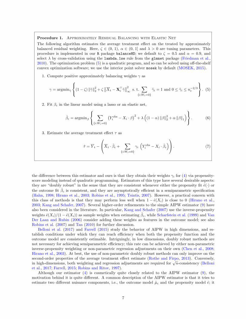
Procedure 1. Approximately Residual Balancing with Elastic Net

The following algorithm estimates the average treatment effect on the treated by approximatelybalanced residual weighting. Here, ζ ∈ (0, 1), α ∈ (0, 1] and λ > 0 are tuning parameters. Thisprocedure is implemented in our R package balanceHD; we default to ζ = 0.5 and α = 0.9, andselect λ by cross-validation using the lambda.1se rule from the glmnet package (Friedman et al.,2010). The optimization problem (5) is a quadratic program, and so can be solved using off-the-shelfconvex optimization software; we use the interior point solver mosek by default (MOSEK, 2015).

1. Compute positive approximately balancing weights γ as

γ = argminγ

(1− ζ) ‖γ‖22 + ζ∥∥Xt −X>c γ

∥∥2∞ s. t.

∑i:Wi=0

γi = 1 and 0 ≤ γi ≤ n−2/3c

. (5)

2. Fit βc in the linear model using a lasso or an elastic net,

βc = argminβ

∑i:Wi=0

(Y obsi −Xi · β

)2+ λ

((1− α) ‖β‖22 + α ‖β‖1

) . (6)

3. Estimate the average treatment effect τ as

τ = Y t −

Xt · βc +∑

i:Wi=0

γi

(Y obsi −Xi · βc

) . (7)

the difference between this estimator and ours is that they obtain their weights γi for (4) via propensity-score modeling instead of quadratic programming. Estimators of this type have several desirable aspects:they are “doubly robust” in the sense that they are consistent whenever either the propensity fit e(·) or

the outcome fit βc is consistent, and they are asymptotically efficient in a semiparametric specification(Hahn, 1998; Hirano et al., 2003; Robins et al., 1995; Tsiatis, 2007). However, a practical concern withthis class of methods is that they may perform less well when 1− e(Xi) is close to 0 (Hirano et al.,2003; Kang and Schafer, 2007). Several higher-order refinements to the simple AIPW estimator (9) havealso been considered in the literature. In particular, Kang and Schafer (2007) use the inverse-propensity

weights e(Xi)/(1− e(Xi)) as sample weights when estimating βc, while Scharfstein et al. (1999) and VanDer Laan and Rubin (2006) consider adding these weights as features in the outcome model; see alsoRobins et al. (2007) and Tan (2010) for further discussion.

Belloni et al. (2017) and Farrell (2015) study the behavior of AIPW in high dimensions, and es-tablish conditions under which they can reach efficiency when both the propensity function and theoutcome model are consistently estimable. Intriguingly, in low dimensions, doubly robust methods arenot necessary for achieving semiparametric efficiency; this rate can be achieved by either non-parametricinverse-propensity weighting or non-parametric regression adjustments on their own (Chen et al., 2008;Hirano et al., 2003). At best, the use of non-parametric doubly robust methods can only improve on thesecond-order properties of the average treatment effect estimate (Rothe and Firpo, 2013). Conversely,in high-dimensions, both weighting and regression adjustments are required for

√n-consistency (Belloni

et al., 2017; Farrell, 2015; Robins and Ritov, 1997).Although our estimator (4) is cosmetically quite closely related to the AIPW estimator (9), the

motivation behind it is quite different. A common description of the AIPW estimator is that it tries toestimate two different nuisance components, i.e., the outcome model µc and the propensity model e; it

7

then achieves consistency if either of these components is itself estimated consistently, and efficiency ifboth components are estimated at fast enough rates. In contrast, our approximate residual balancingestimator bets on linearity twice: once in fitting the outcome model via the lasso, and once in de-biasingthe lasso via balancing weights (5).

By relying more heavily on linearity, we can considerably extend the set of problem under which√n-consistent is possible (assuming linearity in fact holds). As a concrete example, a simple analysis of

AIPW estimation in high-dimensional linear models would start by assuming that the lasso is oP (n−1/4)consistent in root-mean squared error,2 which can be attained via the lasso assuming a k-sparse truemodel with sparsity level k

√n/ log(p); and this is, in fact, exactly the same condition we assume in

Theorem 5. Then, in addition to this requirement on the outcome model, AIPW estimators still needto posit the existence of an oP (n−1/4) consistent estimator of the treatment propensities, whereas we donot need to assume anything about the treatment assignment mechanism beyond overlap. The reasonfor this phenomenon is that the task of balancing (which is all that is needed to correct for the bias ofthe lasso in a linear model) is different from the task of estimating the propensity score—and is in factoften substantially easier.3

2.5 Related Work

Our approximately balancing weights (5) are inspired by the recent litearture on balancing weights (Chanet al., 2015; Deville and Sarndal, 1992; Graham et al., 2012, 2016; Hainmueller, 2012; Hellerstein andImbens, 1999; Hirano et al., 2001; Imai and Ratkovic, 2014; Zhao, 2016). Most closely related, Zubizarreta(2015) proposes estimating τ using the re-weighting formula as in Section 2.2.1 with weights

γ = argminγ

‖γ‖22 subject to

∑γi = 1, γi ≥ 0,

∥∥Xt −X>c γ∥∥∞ ≤ t

, (10)

where the tuning parameter is t; he calls these weights stable balancing weights. These weights are of courseequivalent to ours, the only difference being that Zubizarreta bounds imbalance in constraint form whereaswe do so in Lagrange form. The main conceptual difference between our setting and that of Zubizarreta(2015) is that he considers problem settings where p < nc, and then considers t to be a practically smalltuning parameter, e.g., t = 0.1σ or t = 0.001σ. However, in high dimensions, the optimization problem(10) will not in general be feasible for small values of t; and in fact the bias term

∥∥Xt −X>c γ∥∥∞ becomes

the dominant source of error in estimating τ . We call our weights γ “approximately” balancing in orderto remind the reader of this fact. In settings where it is only possible to achieve approximate balance,weighting alone as considered in Zubizarreta (2015) will not yield a

√n-consistent estimate of the average

treatment effect, and it is necessary to use a regularized regression adjustment as in (4).Similar estimators have been considered by Graham et al. (2012, 2016) and Hainmueller (2012) in

a setting where exact balancing is possible, with slightly different objection functions. For example,

2A more careful analysis of AIPW estimators can trade off the accuracy of the propensity and main effect models and,instead of requiring that both the propensity and outcome models can be estimated at oP (n−1/4) rates, only assumesthat the product of the two rates be bounded as oP (n−1/2); see, e.g., Farrell (2015). In high dimensions, this amounts toassuming that the outcome and propensity models are both well specified and sparse, with respective sparsity levels kβ andke satisfying kβke n/ log(p)2. AIPW can thus be preferable to ARB given sparse enough and well specified propensitymodels, with ke

√n/ log(p).

3The above distinctions all relied on a presupposition that that we are in a situation where the statistician starts witha set of high-dimensional covariates, and needs to find a way to control for all of them at once. In this setting, linearityis a strong assumption, and so it is not surprising that making this assumption lets us considerably weaken requirementson other aspects of the problem. In other applications, however, the statistician may have started with low-dimensionaldata, but then created a high-dimensional design by listing series expansions of the original data, interactions, etc. In thissetting, linearity becomes a non-assumption (since any smooth function can be well approximated using a large enoughnumber terms from an appropriately chosen series expansion), and we should expect our approach to perform comparablyto doubly robust methods. Wang and Zubizarreta (2017) provide a formal result of this type, and establish conditions underwhich approximately balancing weights γi in fact converge to the oracle inverse-propensity weights e(Xi)/(1 − e(Xi)). Inother words, their results imply that, if we obtain the design matrix Xc via a series expansion, then—under regularityconditions—approximate residual balancing is also doubly robust, and asymptotically equivalent to AIPW.

8

Hainmueller (2012) uses −∑i ln(γi) instead of

∑i γ

2i , leading to

γ = argminγ

− ∑i:Wi=0

log (γi) subject to∑

γi = 1, γi ≥ 0,∥∥Xt −X>c γ

∥∥∞ = 0

. (11)

This estimator has attractive conceptual connections to logistic regression and maximum entropy esti-mation, and in a low dimensional setting where W |X admits a well-specified logistic model the methodsof Graham et al. (2012, 2016) and Hainmueller (2012) are doubly robust (Hirano et al., 2001; Imbenset al., 1998; Newey and Smith, 2004). In terms of our immediate concerns, however, the variance ofτ depends on γ through ‖γ‖22 and not −

∑log (γi), so our approximately balancing weights are more

directly induced by our statistical objective than those defined in (11).Finally, in this paper, we have emphasized an asymptotic analysis point of view, where we evalu-

ate estimators via their large sample accuracy. From this perspective, our estimator—which combinesweighting with a regression adjustment as in (4)—appears to largely dominate pure weighting estima-tors; in particular, in high dimensions, we achieve

√n-consistency whereas pure weighting estimators

do not. On the other hand, stressing practical concerns, Rubin (2008) strongly argues that “designedbased” inference leads to more credible conclusions in applications by better approximating randomizedexperiments. In our context, design based inference amounts to using a pure weighting estimator of theform

∑γiYi where the γi are chosen without looking at the Yi. The methods considered by Chan et al.

(2015), Graham et al. (2012), Hainmueller (2012), Zubizarreta (2015), etc., all fit within this design-basedparadigm, whereas ours does not.

3 Asymptotics of Approximate Residual Balancing

3.1 Approximate Residual Balancing as Debiased Linear Estimation

As we have already emphasized, approximate residual balancing is a method that enables us to makesinferences about average treatment effects without needing to estimate treatment propensities as nuisanceparameters; rather, we build on recent developments on inference in high-dimensional linear models (Caiand Guo, 2015; Javanmard and Montanari, 2014, 2015; Ning and Liu, 2014; Van de Geer et al., 2014;Zhang and Zhang, 2014). Our main goal is to understand the asymptotics our estimates for µc = Xt·βc. Inthe interest of generality, however, we begin by considering a broader problem, namely that of estimatinggeneric contrasts ξ ·βc in high-dimensional linear models. This detour via linear theory will help highlightthe statistical phenomena that make approximate residual balancing work, and explain why—unlike themethods of Belloni et al. (2017), Chernozhukov et al. (2017) or Farrell (2015)—our method does notrequire consistent estimability of the treatment propensity function e(x).

The problem of estimating sparse linear contrasts ξ · βc in high-dimensional regression problemshas received considerable attention, including notable recent contributions by Javanmard and Montanari(2014, 2015), Van de Geer et al. (2014), and Zhang and Zhang (2014). These papers, however, exclusivelyconsider the setting where ξ is a sparse vector, and, in particular, focus on the case where ξ is the j-thbasis vector ej , i.e., the target estimand is the j-th coordinate of βc. But, in our setting, the contrastvector Xt defining our estimand µc = Xt · βc is random and thus generically dense; moreover, we areinterested in applications where mt = E[Xt] itself may also be dense. Thus, a direct application of thesemethod is not appropriate in our problem.4

An extension of this line of work to the problem of estimating dense, generic contrasts θ = ξ ·βc turnsout to be closely related to our approximate residual balancing method for treatment effect estimation.

4As a concrete example, Theorem 6 of Javanmard and Montanari (2014) shows that their debiased estimator β(debiased)c

satisfies√nc(β

(debiased)c − βc) = Z + ∆, where Z is a Gaussian random variable with desirable properties and ‖∆‖∞ = o(1).

If we simply consider sparse contrasts of βc, then this error term ∆ is negligible; however, in our setting, we would have aprohibitively large error term Xt ·∆ that may grow polynomially in p.

9

To make this connection explicit, define the following estimator:

θ = ξ · βc +∑

i:Wi=0

γi

(Y obsi −Xi · βc

), where (12)

γ = argminγ

‖γ‖22 subject to∥∥ξ −X>c γ

∥∥∞ ≤ K

√log(p)

nc, max

i|γi| ≤ n−2/3c

, (13)

βc is a properly tuned sparse linear estimator, and K is a tuning parameter discussed below. If we set ξ ←Xt, then this estimator is nothing but our treatment effect estimator from Procedure 1.5 Conversely, inthe classical parameter estimation setting with ξ ← ej , the above procedure is algorithmically equivalentto the one proposed by Javanmard and Montanari (2014, 2015). Thus, the estimator (12) can be thoughtof as an adaptation of the method of Javanmard and Montanari (2014, 2015) that debiases βc specificallyalong the direction of interest ξ.

We begin our analysis in Section 3.2 by considering a general version of (12) under fairly strong“transformed independence design” generative assumptions on Xc. Although these assumptions maybe too strong to be palatable in practical data analysis, this result lets us make a crisp conceptual linkbetween approximate residual balancing and the debiased lasso. In particular, we find that (Theorem 3), θfrom (12) is

√n-consistent for θ provided ξ>Σ−1c ξ = O(1), where Σc is the covariance of Xc. Interestingly,

if Σc = Ip×p, then in general ξ>Σ−1c ξ = ‖ξ‖22 = O(1) if and only if ξ is very sparse, and so the classicalde-biased lasso theory reviewed above is essentially sharp despite only considering the sparse-ξ case (seealso Cai and Guo, 2015). On the other hand, whenever Σc has latent correlation structure, it is possibleto have ξ>Σ−1c ξ = O(1) even when ξ is dense and ‖ξ‖2 1, provided that ξ is aligned with the largelatent components of Σc. We also note that, in the application to treatment effect estimation, X

>t Σ−1c Xt

will in general be much larger than 1; however, in Corollary 4 we show how to overcome this issue.To our knowledge, this was the first result for

√n-consistent inference about dense contrasts of βc at

the time we first circulated our manuscript. We note, however, simultaneous and independent work byZhu and Bradic (2016), who developed a promising method for testing hypotheses of the form ξ · βc = 0for potentially dense vectors ξ; their approach uses an orthogonal moments construction that relies onregressing ξ ·Xi against a p− 1 dimensional design that captures the components of Xi orthogonal to ξ.

Finally, in Section 3.3, we revisit the specific problem of high-dimensional treatment effect estimationvia approximate residual balancing under substantially weaker assumptions on the design matrix Xc:Rather than assuming a generative “transformed independence design” model, we simply require overlapand standard regularity conditions. The cost of relaxing our assumptions on Xc is that we now getslightly looser performance guarantees; however, our asymptotic error rates are still in line with those wecould get from doubly robust methods. We also discuss practical, heteroskedasticity-robust confidenceintervals for τ . Through our analysis, we assume that βc is obtained via the lasso; however, we could justas well consider, e.g., the square-root lasso (Belloni et al., 2011), sorted L1-penalized regression (Bogdanet al., 2015; Su and Candes, 2016), or other methods with comparable L1-risk bounds.

3.2 Debiasing Dense Contrasts

As we begin our analysis of θ defined in (12), it is first important to note that the optimization program(13) is not always feasible. For example suppose that p = 2nc, that Xc = (Inc×nc

Inc×nc), and that

ξ consists of n times “1” followed by n times “−1”; then∥∥ξ −X>c γ

∥∥∞ ≥ 1 for any γ ∈ Rnc , and the

approximation error does not improve as nc and p both get large. Thus, our first task is to identify aclass of problems for which (13) has a solution with high probability. The following lemma establishessuch a result for random designs, in the case of vectors ξ for which ξ>Σ−1c ξ is bounded; here Σc =Var

[Xi

∣∣Wi = 0]

denotes the population variance of control features. We also rely on the following

5Here, we phrased the imbalance constraint in constraint form rather that in Lagrange form; the reason for this is that,although there is a 1:1 mapping between these two settings, we found the former easier to work with formally whereas thelatter appears to yield more consistent numerical performance. We also dropped the constraints

∑γi = 1 and γi ≥ 0 for

now, but will revisit them in Section 3.3.

10

regularity condition, which will be needed for an application of the Hanson-Wright concentration boundfor quadratic forms following Rudelson and Vershynin (2013).

Assumption 3 (Transformed Independence Design). Suppose that we have a sequence of random designproblems with6 Xc = QΣ

12c , where E [Qij ] = 0, Var [Qij ] = 1, for all indices i and j, and the individual

entries Qij are all independent. Moreover suppose that the Q-matrix is sub-Gaussian for some ς > 0,E [exp [t (Qij − E [Qij ])]] ≤ exp

[ς2t2/2

]for any t > 0, and that (Σc)jj ≤ S for all j = 1, ..., p.

Lemma 2. Suppose that we have a sequence of problems for which Assumption 3 holds and, moreover,ξ>Σ−1c ξ ≤ V for some constant V > 0. Then, there is a universal constant C > 0 such that, settingK = Cς2

√V S, the optimization problem (13) is feasible with probability tending to 1; and, in particular,

the constraints are satisfied by γ∗i = 1ncξ>Σ−1c Xi.

The above lemma is the key to our analysis of approximate residual balancing. Because, with highprobability, the weights γ∗ from Lemma 2 provide one feasible solution to the constraint in (13), weconclude that, again with high probability, the actual weights we use for approximate residual balancingmust satisfy ‖γ‖22 ≤ ‖γ∗‖

22 ≈ n−1c ξ>Σ−1c ξ. In order to turn this insight into a formal result, we need

assumptions on both the sparsity of the signal and the covariance matrix Σc.

Assumption 4 (Sparsity). We have a sequence of problems indexed by n, p, and k such that theparameter vector βc is k-sparse, i.e., ‖βc‖0 ≤ k, and that k log(p)/

√n→ 0.7

The above sparsity requirement is quite strong. However, many analyses that seek to establish asymp-totic normality in high dimensions rely on such an assumption. For example, Javanmard and Montanari(2014), Van de Geer et al. (2014), and Zhang and Zhang (2014) all make this assumption when seekingto provide confidence intervals for individual components of βc; Belloni et al. (2014) use a similar as-sumption where they allow for additional non-zero components, but they assume that beyond the largestk components with k satisfying the same sparsity condition, the remaining non-zero elements of βc aresufficiently small that they can be ignored, in what they refer to as approximate sparsity.8

Next, our analysis builds on well-known bounds on the estimation error of the lasso (Bickel et al.,2009; Hastie et al., 2015) that require Xc to satisfy a form of the restricted eigenvalue condition. Below,we make a restricted eigenvalue assumption on Σ

1/2c ; then, we will use results from Rudelson and Zhou

(2013) to verify that this also implies a restricted eigenvalue condition on Xc.

Assumption 5 (Well-Conditioned Covariance). Given the sparsity level k specified above, the covariance

matrix Σ1/2c of the control features satisfies the k, 2ω, 10-restricted eigenvalue defined as follows, for

some ω > 0. For 1 ≤ k ≤ p and L ≥ 1, define the set Ck(L) as

Ck(L) =

β ∈ Rp : ‖β‖1 ≤ Lk∑j=1

∣∣βij ∣∣ for some 1 ≤ i1 < ... < ij ≤ p

. (14)

Then, Σ1/2c satisfies the k, ω, L-restricted eigenvalue condition if β>Σcβ ≥ ω ‖β‖22 for all β ∈ Ck(L).

6In order to simplify our exposition, this assumption implicitly rules out the use of an intercept. Our analysis would gothrough verbatim, however, if we added an intercept X1 = 1 to the design.

7In recent literature, there has been some interest in methods that require only require approximate, rather than exact,k-sparsity. We emphasize that our results also hold with approximate rather than exact sparsity, as we only use our sparsityassumption to get bounds on ‖βc − βc‖1 that can be used in conjunction with Proposition 1. For simplicity of exposition,however, we restrict our present discussion to the case of exact sparsity.

8There are, of course, some exceptions to this assumption. In recent work, Javanmard and Montanari (2015) show thatinference of βc is possible even when k n / log(p) in a setting where X is a random Gaussian matrix with either aknown or extremely sparse population precision matrix; Wager et al. (2016) show that lasso regression adjustments allowfor efficient average treatment effect estimation in randomized trials even when k n / log(p); while the method of Zhuand Bradic (2016) for estimating dense contrasts ξ · βc does not rely on sparsity of βc, and instead places assumptions onthe joint distribution of ξ ·Xi and the individual regressors. The point in common between these results is that they let usweaken the sparsity requirements at the expense of strengthening our assumptions about the X-distribution.

11

Theorem 3. Under the conditions of Lemma 2 hold, suppose that the control outcomes Yi(0) are drawnfrom a sparse, linear model as in Assumptions 1, 2, 3 and 4, that Σ

1/2c satisfies the restricted eigenvalue

property (Assumption 5), and that we have a minimum estimand size9 ‖ξ‖∞ ≥ κ > 0. Suppose, moreover,that we have homoskedastic noise: Var[εi(0)

∣∣Xi] = σ2 for all i = 1, ..., n, and also that the response noiseεi(0) := Yi(0)− E[Yi(0)

∣∣Xi] is uniformly sub-Gaussian with parameter υ2S > 0. Finally, suppose thatwe estimate θ using (12), with the optimization parameter K selected as in Lemma 2 and the lasso penalty

parameter set to λn = 5ς2υ√

log (p) /nc. Then, θ is asymptotically Gaussian,(θ − θ

) /‖γ‖2 ⇒ N

(0, σ2

), nc ‖γ‖22

/ξ>Σ−1c ξ ≤ 1 + op(1). (15)

The statement of Theorem 3 highlights a connection between our debiased estimator (12), and theordinary least-squares (OLS) estimator. Under classical large-sample asymptotics with n p, it is wellknown that the OLS estimator, θ(OLS) = ξ>(X>c Xc)

−1X>c Y , satisfies

√nc

(θ(OLS) − θ

) /√ξ>Σ−1c ξ ⇒ N

(0, σ2

), and

√nc

θ(OLS) − θ − ∑i:Wi=0

γ∗i εi(0)

→p 0, (16)

where γ∗i is as defined in Lemma 2. By comparing this characterization to our result in Theorem 3, itbecomes apparent that our debiased estimator θ has been able to recover the large-sample qualitativebehavior of θ(OLS), despite being in a high-dimensional p n regime. The connection between debiasingand OLS ought not appear too surprising. After all, under classical assumptions, θ(OLS) is known to bethe minimum variance unbiased linear estimator for θ; while the weights γ in (13) were explicitly chosento minimize the variance of θ subject to the estimator being nearly unbiased.

A downside of the above result is that our main goal is to estimate µc = Xt · βc, and this contrast-defining vector Xt fails to satisfy the bound on X

>t Σ−1Xt assumed in Theorem 3. In fact, because Xt

is random, this quantity will in general be on the order of p/n. In the result below, we show how to getaround this problem under the weaker assumption that m>t Σ−1c mt is bounded; at a high level, the proofshows that the the stochasticity Xt does not invalidate our previous result. We note that, because Y t

is uncorrelated with µc conditionally on Xt, the following result also immediately implies a central limittheorem for τ = Y t − µc where Y t is the average of the treated outcomes.

Corollary 4. Under the conditions of Theorem 3, suppose that we want to estimate µc = Xt · βcby replacing ξ with Xt in (12), and let mt = E

[X∣∣W = 1

]. Suppose, moreover, that we replace all

the assumptions made about ξ in Theorem 3 with the following assumptions: throughout our sequenceof problems, the vector mt satisfies mtΣ

−1c mt ≤ V and ‖mt‖∞ ≥ κ. Suppose, finally, that (Xi −

mt)j∣∣Wi = 1 is sub-Gaussian with parameter ν2 > 0, and that the overall odds of receiving treatment

P [W = 1] /P [W = 0] tend to a limit ρ bounded away from 0 and infinity. Then, setting the tuningparameter in (13) as K = Cς2

√V S + ν

√2.1 ρ, we get

(µc − µc)/‖γ‖2 ⇒ N

(0, σ2

), nc ‖γ‖22

/m>t Σ−1c mt ≤ 1 + op(1). (17)

The asymptotic variance bound m>t Σ−1c mt is exactly the Mahalanobis distance between the meantreated and control subjects with respect to the covariance of the control sample. Thus, our resultshows that we can achieve asymptotic inference about τ with a 1/

√n rate of convergence, irrespective of

the dimension of the features, subject only to a requirement on the Mahalanobis distance between thetreated and control classes, and comparable sparsity assumptions on the Y -model as used by the restof the high-dimensional inference literature, including Belloni et al. (2014, 2017), Chernozhukov et al.(2017) and Farrell (2015). However, unlike this literature, we make no assumptions on the propensitymodel beyond overlap, and do not require it to be estimated consistently. In other words, by relyingmore heavily on linearity of the outcome function, we can considerably relax the assumptions requiredto get

√n-consistent treatment effect estimation.

9The minimum estimand size assumption is needed to rule out pathological superefficient behavior. As a concreteexample, suppose that Xi ∼ N (0, Ip×p), and that ξj = 1/

√p for j = 1, ..., p with p nc. Then, with high probability,

the optimization problem (13) will yield γ = 0. This leaves us with a simple lasso estimator θ = ξ · βc whose risk scalesas E[(θ − θ)2] = O(k2 log(p)/(pnc)) 1/nc. The problem with this superefficient estimator is that it is not necessarilyasymptotically Gaussian.

12

3.3 A Robust Analysis with Overlap

Our discussion so far, leading up to Corollary 4, gives a characterization of when and why we shouldexpect approximate residual balancing to work. However, from a practical perspective, the assumptionsused in our derivation—in particular the transformed independence design assumption—were strongerthan ones we may feel comfortable making in applications.

In this section, we propose an alternative analysis of approximate residual balancing based on overlap.Informally, overlap requires that each unit have a positive probability of receiving each of the treatmentand control conditions, and thus that the treatment and control populations cannot be too dissimilar.Without overlap, estimation of average treatment effects relies fundamentally on extrapolation beyond thesupport of the features, and thus makes estimation inherently sensitive to functional form assumptions;and, for this reason, overlap has become a common assumption in the literature on causal inferencefrom observational studies (Crump et al., 2009; Imbens and Rubin, 2015). For estimation of the averageeffect for the treated we in fact only need the propensity score to be bounded from above by 1− η, butfor estimation of the overall average effect we would require both the lower and upper bound on thepropensity score. If we are willing to assume overlap, we can relax the transposed independence designassumption into much more routine regularity conditions on the design, as in Assumption 7.

Assumption 6 (Overlap). There is a constant 0 < η such that η ≤ e(x) ≤ 1− η for all x ∈ Rp.

Assumption 7 (Design). Our design X satisfies the following two conditions. First, the design is sub-Gaussian, i.e., there is a constant ν > 0 such that the distribution of Xj conditional on W = w issub-Gaussian with parameter ν2 after re-centering. Second, we assume that Xc satisfies the k, ω, 4-restricted eigenvalue condition as defined in Assumption 5, with probability tending to 1.

Following Lemma 2, our analysis again proceeds by guessing a feasible solution to (29), and thenusing it to bound the variance of our estimator. Here, however, we using inverse-propensity weights asour guess: γ∗i ∝ e(Xi)/(1−e(Xi)). Our proof hinges on showing that the actual weights we get from (29)are at least as good as these inverse-propensity weights, and thus our method will be at most as variableas one that uses augmented inverse-propensity weighting (9) with these oracle propensity weights.

Theorem 5. Suppose that we have n independent and identically distributed training examples satisfyingAssumptions 1, 2, 4, 6, 7, and that the treatment odds P [W = 1] /P [W = 0] converge to ρ with 0 <ρ < ∞. Suppose, moreover, that we have homoskedastic noise: Var[εi(w)

∣∣Xi] = σ2 for all i = 1, ..., n,and also that the response noise εi(w) := Yi(w)− E[Yi(w)

∣∣Xi] is uniformly sub-Gaussian with parameterυ2 > 0. Finally, suppose that we use (4) with weights (5), except we replace the Lagrange-form penalty onthe imbalance with a hard constraint ‖Xt −X>c γ‖∞ ≤ K

√log(p)/nc, with K = ν

√2.1(ρ+ (η−1 − 1)2.

Moreover, we fit the outcome model using a lasso with penalty parameter set to λn = 5νυ√

log (p) /nc.Then,

µc − µc

‖γ‖2⇒ N

(0, σ2

)and

τ − τ√n−1t + ‖γ‖22

⇒ N(0, σ2

), (18)

where τ is the expected treatment effect on the treated (2). Moreover,

lim supn→∞

nc ‖γ‖22 ≤ ρ−2 E

[(e (Xi)

1− e (Xi)

)2∣∣∣∣∣Wi = 0

]. (19)

The rate of convergence guaranteed by (19) is the same as what we would get if we actually knewthe true propensities and could use them for weighting (Robins et al., 1994, 1995). Here, we achieve thisrate although we have no guarantees that the true propensities e(Xi) are consistently estimable. Finally,we note that, when the assumptions to Corollary 4 hold, the bound (17) is stronger than (19); however,there exist designs where the bounds match (Wang and Zubizarreta, 2017).

Finally, in applications, it is often of interest to have confidence intervals for µc and τ rather than justpoint estimates; below, we propose such a construction. Much like the sandwich variance estimates for or-dinary least squares regression, our proposed confidence intervals are heteroskedaticity robust even though

13

the underlying point estimates were motivated using an argument written in terms of a homoskedasticsampling distribution.

Corollary 6. Under the conditions of Theorems 3 or 5, suppose instead that we have heteroskedasticnoise υ2min ≤ Var

[εi(Wi)

∣∣Xi, Wi

]≤ υ2 for all i = 1, ..., n. Then, the following holds:

(µc − µc)/√

Vc ⇒ N (0, 1) , Vc =∑

i:Wi=0

γ2i

(Yi −Xi · βc

)2. (20)

In order to provide inference about τ , we also need error bounds for µt. Under sparsity assumptionscomparable to those made for βc in Theorem 5, we can verify that

(µt − µt)/√

Vt ⇒ (0, 1) , Vt =1

n2t

∑i:Wi=1

(Yi −Xiβt

)2, (21)

where βt is obtained using the lasso with λn = 5νυ√

log (p) /nc. Moreover, µc and µt are independentconditionally on X and W , thus implying that (τ − τ) / (Vc + Vt)

1/2 ⇒ N (0, 1). This last expression iswhat we use for building confidence intervals for τ .

4 Application: The Efficacy of Welfare-to-Work Programs

Starting in 1986, California implemented the Greater Avenues to Independence (GAIN) program, withan aim to reduce dependence on welfare and promote work among disadvantaged households. The GAINprogram provided its participats with a mix of educational resources such as English as a second languagecourses and vocational training, and job search assistance. This program is described in detail by Hotzet al. (2006). In order to evaluate the effect of GAIN, the Manpower Development Research Corporationconducted a randomized study between 1988 and 1993, where a random subset of GAIN registrants wereeligible to receive GAIN benefits immediately, whereas others were embargoed from the program until1993 (after which point they were allowed to participate in the program). All experimental subjects werefollowed for a 3-year post-randomization period.

The randomization for the GAIN evaluation was conducted separately by county; following Hotz et al.(2006), we consider data from Alameda, Los Angeles, Riverside and San Diego counties. As discussedin detail in Hotz et al. (2006), the experimental conditions differed noticeably across counties, both interms of the fraction of registrants eligible for GAIN, i.e., the treatment propensity, and in terms of thesubjects participating in the experiment. For example, the GAIN programs in Riverside and San Diegocounties sought to register all welfare cases in GAIN, while the programs in Alameda and Los Angelescounties focused on long-term welfare recipients.

The fact that the randomization of the GAIN evaluation was done at the county level rather thanat the state level presents us with a natural opportunity to test our method, as follows. We seek toestimate the average treatment effect of GAIN on the treated; however, we hide the county informationfrom our procedure, and instead try to compensate for sampling bias by controlling for a large amount ofcovariates. We used spline expansions of age and prior income, indicators for race, family status, etc., fora total of p = 93 covariates. Meanwhile, we can check our performance against a gold standard estimateof the average treatment effect that is stratified by county and thus guaranteed to be unbiased.10

We compare the behavior of different methods for estimating the average treatment effect on thetreated using randomly drawn subsamples of the original data (the full dataset has n = 19, 170). Inaddition to approximate residual balancing, we consider augmented inverse-propensity weighting (9) and

10More formally, in our experiments, we set the gold standard using the county-stratified oracle estimator on bootstrapsamples of the full n = 19, 170 sample. We use bootstrap samples to correct for the correlation of estimators τ obtainedusing the full dataset and subsamples of it. We also note that, given this setup, the quantity we are using as our goalstandard is not and estimate of τ , i.e., the conditional average treatment effect on the treated sample, and should ratherbe thought of as an estimate of E [τ ], i.e., the average treatment effect on the treated population. Since we are in a settingwith a fairly weak signal, this should not make a noticeable difference in practice.

14

200 500 1000 2000 5000

0.80

0.85

0.90

0.95

n

Cov

erag

e

Oracle AdjustmentApprox. Resid. BalanceDouble Select + OLSAugmented IPWNo Adjustment (Naive)

200 500 1000 2000 5000

0.00

50.

010

0.02

00.

050

0.10

0

n

MS

E

Oracle AdjustmentApprox. Resid. BalanceDouble Select + OLSAugmented IPWNo Adjustment (Naive)

Coverage Mean-Squared Error

Figure 1: Finite sample performance of the average treatment effect on the treated for different estimators,aggregated over 1,000 replications. The target coverage rate, 0.95, is denoted with a dotted line.

double selection following Belloni et al. (2014) as our baselines. We also show the behavior of an “oracle”procedure that gets to observe the hidden county information and then simply estimates treatment effectsfor each county separately, and the “naive” difference-in-means estimator that ignores the features X. Invery small samples, the oracle procedure is not always well defined because some samples may result incounties where either everyone or no one is treated.

Figure 1 compares the performance of the different methods. We see that approximate residualbalancing and double selection both do well in terms of mean-squared error. Moreover, confidence intervalsbuilt via approximate residual balancing achieve effectively nominal coverage; double selection also getsreasonable coverage and improves with n. In contrast, augmented inverse-propensity weighting does notperform well here. The problem appears to be that estimating treatment propensities is quite difficult,and a cross-validated logistic elastic net often learns an effectively constant propensity model.

5 Simulation Experiments

5.1 Methods under Comparison

In addition to approximate residual balancing as described in Procedure 1, the methods we use asbaselines are as follows: naive difference-in-means estimation τ = Y t − Y c that ignores the covariateinformation X; the elastic net (Zou and Hastie, 2005), or equivalently, Procedure 1 with trivial weightsγi = 1/nc; approximate balancing, or equivalently, Procedure 1 with trivial parameter estimates βc = 0(Zubizarreta, 2015); inverse-propensity weighting, as discussed in Section 2.2.1, with propensityestimates e(Xi) obtained by elastic net logistic regression, with the propensity scores trimmed at 0.05and 0.95; augmented inverse-propensity weighting, which pairs elastic net regression adjustmentswith the above inverse-propensity weights (9); the weighted elastic net, motivated by Kang and Schafer(2007), that uses inverse-propensity weights as sample weights for the elastic net regression; targetedmaximum likelihood estimation (TMLE), which fine-tunes the elastic net regression estimates alongthe direction specified by the inverse-propensity weights (Van Der Laan and Rubin, 2006), and ordinaryleast squares after model selection where, in the spirit of Belloni et al. (2014), we run lasso linearregression for Y

∣∣X, W = 0 and lasso logistic regression for W∣∣X, and then compute the ordinary least

squares estimate for τ on the union of the support of the three lasso problems.Unless otherwise specified, all outcome and propensity models were fit using a (linear or logistic)

elastic net. Whenever there is a “λ” regularization parameter to be selected, we use cross validation withthe lambda.1se rule from the glmnet package (Friedman et al., 2010). In Belloni et al. (2014), the authors

15

−15 −10 −5 0 5

−5

05

10

(a) Low-dimensional version of the many clus-ters simulation setting. The blue and red dotsdenote control and treated X-observations re-spectively.

−2 −1 0 1 2

0.0

0.1

0.2

0.3

0.4

0.5

X

Treatment EffectDistr. of TreatedDistr. of Controls

(b) Schematic of misspecified simulation set-ting, along the first covariate (Xi)1. The“treatment effect” curve is not to scale alongthe Y -axis.

Figure 2: Illustrating simulation designs.

recommend selecting λ using more sophisticated methods, such as the square-root lasso (Belloni et al.,2011). However, in our simulations, our implementation of Belloni et al. (2014) still attains excellentperformance in the regimes the method is designed to work in. Similarly, our confidence intervals forτ are built using a cross-validated choice of λ instead of the fixed choice assumed by Corollary 6. Ourimplementation of approximate residual balancing, as well as all the discussed baselines, is available inthe R-package balanceHD.

5.2 Simulation Designs

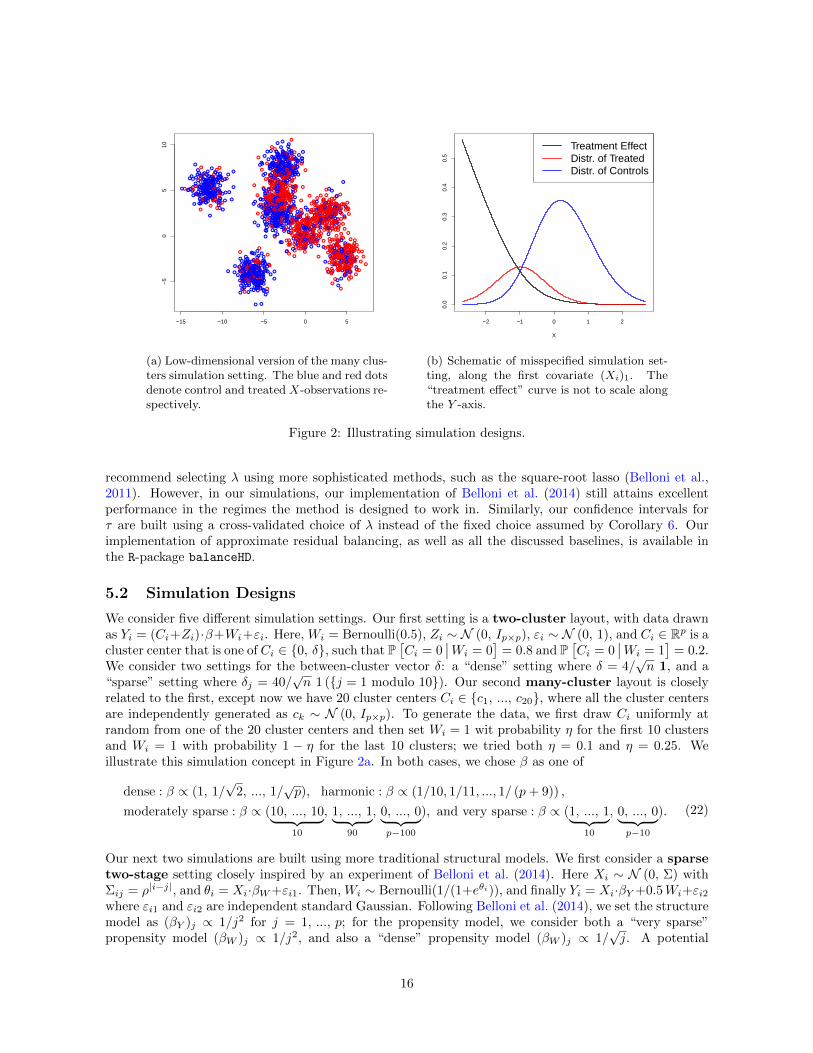
We consider five different simulation settings. Our first setting is a two-cluster layout, with data drawnas Yi = (Ci+Zi)·β+Wi+εi. Here, Wi = Bernoulli(0.5), Zi ∼ N (0, Ip×p), εi ∼ N (0, 1), and Ci ∈ Rp is acluster center that is one of Ci ∈ 0, δ, such that P

[Ci = 0

∣∣Wi = 0]

= 0.8 and P[Ci = 0

∣∣Wi = 1]

= 0.2.We consider two settings for the between-cluster vector δ: a “dense” setting where δ = 4/

√n 1, and a

“sparse” setting where δj = 40/√n 1 (j = 1 modulo 10). Our second many-cluster layout is closely

related to the first, except now we have 20 cluster centers Ci ∈ c1, ..., c20, where all the cluster centersare independently generated as ck ∼ N (0, Ip×p). To generate the data, we first draw Ci uniformly atrandom from one of the 20 cluster centers and then set Wi = 1 wit probability η for the first 10 clustersand Wi = 1 with probability 1 − η for the last 10 clusters; we tried both η = 0.1 and η = 0.25. Weillustrate this simulation concept in Figure 2a. In both cases, we chose β as one of

dense : β ∝ (1, 1/√

2, ..., 1/√p), harmonic : β ∝ (1/10, 1/11, ..., 1/ (p+ 9)) ,

moderately sparse : β ∝ (10, ..., 10︸ ︷︷ ︸10

, 1, ..., 1︸ ︷︷ ︸90

, 0, ..., 0︸ ︷︷ ︸p−100

), and very sparse : β ∝ (1, ..., 1︸ ︷︷ ︸10

, 0, ..., 0︸ ︷︷ ︸p−10

). (22)

Our next two simulations are built using more traditional structural models. We first consider a sparsetwo-stage setting closely inspired by an experiment of Belloni et al. (2014). Here Xi ∼ N (0, Σ) withΣij = ρ|i−j|, and θi = Xi·βW+εi1. Then, Wi ∼ Bernoulli(1/(1+eθi)), and finally Yi = Xi·βY +0.5Wi+εi2where εi1 and εi2 are independent standard Gaussian. Following Belloni et al. (2014), we set the structuremodel as (βY )j ∝ 1/j2 for j = 1, ..., p; for the propensity model, we consider both a “very sparse”propensity model (βW )j ∝ 1/j2, and also a “dense” propensity model (βW )j ∝ 1/

√j. A potential

16

criticism of this simulation design is that the signal is perhaps unusually sparse (in the 4-th column ofTable 3, adjusting for differences in the two most important covariates removes 93% of the bias associatedwith all the covariates); moreover, we note that all the important coefficients of both βY and βW are closeto each other in terms of their indices; thus, the effect of using a correlated design may be mitigated. Thus,we also ran a moderately sparse two-stage simulation, just like the above one, except we now usedchoices for βY as in (22), the only difference being that we shifted the indices of the betas, multiplyingthem by 23 mod p (e.g., the harmonic setup now has (β)j ∝ 1/[10+(23 (j−1) mod p)]). Here, we drew the

treatment assignments from a well-specified logistic model, Wi ∼ Bernoulli(1/(1+exp(−∑100j=1Xij/40))).

To test the robustness of all considered methods, we also ran a misspecified simulation. Here, wefirst drew Xi ∼ N (0, Ip×p), and defined latent parameters θi = log(1 + exp(−2 − 2 ∗ (Xi)1))/0.915.We then drew Wi ∼ Bernoulli(1 − e−θi), and finally Yi = (Xi)1 + · · · + (Xi)10 + θi(2Wi − 1)/2 + εiwith εi ∼ N (0, 1). We varied n and p. This simulation setting, loosely inspired by the classic programevaluation dataset of LaLonde (1986), is illustrated in Figure 2b; note that the average treatment effecton the treated is much greater than the overall average treatment effect here.

5.3 Results

In the first two experiments, for which we report results in Tables 1 and 2, the outcome model Y |X isreasonably sparse, while the propensity model has overlap but is not in general sparse. In relative terms,this appears to hurt the double-selection method most. Meanwhile, in Table 3, we find that the methodof Belloni et al. (2014) has excellent performance—as expected—when both the propensity and outcomemodels are sparse. However, if we make the problem somewhat more difficult (Table 4), its performancedecays substantially, and double selection lags both approximate residual balancing and propensity-basedmethods in its performance.

Generally, we find that the balancing performs substantially better than propensity score weighting,with or without direct covariate adjustment. We also find that combining direct covariate adjustmentwith weighting does better than weighting on its own, irrespective of whether the weighting is basedon balance or on the propensity score. In these experiments, the weighted elastic net and TMLE alsosomewhat improve over AIPW.

Encouragingly, approximate residual balancing also does a good job in the misspecified setting fromTable 5. It appears that our stipulation that the approximately balancing weights (5) must be non-negative (i.e., γi ≥ 0) helps prevent our method from extrapolating too aggressively. Conversely, leastsquares with model selection does not perform well despite both the outcome and propensity modelsbeing sparse; apparently, it is more sensitive to the misspecification here. Perhaps the reason AIPW andTMLE do not do as well here is that there are very strong linear effects.

We evaluate coverage of confidence intervals in the “many-cluster” setting for different choices of β, n,and p; results are given in Table 6. Coverage is generally better with more overlap (η = 0.25) rather thanless (η = 0.1), and with sparser choices of β. Moreover, coverage rates appear to improve as n increases,suggesting that we are in a regime where the asymptotics from Corollary 6 are beginning to apply.

6 Discussion

In this paper, we introduced approximate residual balancing as a method for unconfounded averagetreatment effect estimation in high-dimensional linear models. Under standard assumptions from thehigh-dimensional inference literature, our method allows for

√n-consistent inference of the average treat-

ment effect without any structural assumptions on the treatment assignment mechanism beyond overlap.Widely used doubly robust methods, pioneered by Robins et al. (1994) and studied further by several

authors (e.g., Belloni et al., 2017; Farrell, 2015; Kang and Schafer, 2007; Scharfstein et al., 1999; Robinset al., 2007; Tan, 2010; Van Der Laan and Rubin, 2006), approach this problem by trying to estimate twodifferent nuisance components, the outcome model and the propensity model. These methods then achieveconsistency if either nuisance component is itself consistently estimated, and achieve semiparametricefficiency if both components as estimated fast enough. In contrast, our method “bets” on linearity

17

twice, both in fitting the lasso and in attempting to balance away its bias. In well specified linear models,this bet allows us to considerably extend the class of problems for with

√n-consistent inference of average

treatment effects is possible; thus, if a practitioner believes linearity to be a reasonable assumption in agiven problem, our estimator may be a promising choice.

We end by mentioning two important questions left open by this paper. First, it would be importantto develop a better understanding of how to choose the tuning parameter ζ in (5) that trades off biasand variance in our balancing. Results from Theorems 3 and 5 provide some guidance on choosing ζ(via a constraint-form characterization); however, in our experiments, we achieved good performanceby simply setting ζ = 1/2 everywhere. The difficulty in choosing ζ is that we are trying to trade offan observable quantity (sampling variance) against an unobservable one (residual bias), and so cannotrely on simple methods like cross-validation that require unbiased estimates of the loss criterion we aretrying to minimize. It would be of considerable interest to either devise a data-adaptive choice for ζ, orunderstand why a fixed choice ζ = 1/2 appears to achieve systematically good performance.

It would also be interesting to extend our approach to generalized linear models, where there is a non-linear link function ψ for which E[Yi(c)

∣∣Xi = x] = ψ(x · βc). In causal inference applications, this settingfrequently arises when the outcomes Y obs

i are binary, and we are willing to work with a logistic regressionmodel. In this case, the first-order error component from using a pilot estimator βc for estimating µc witha plug-in estimator n−1c

∑Wi=1 ψ(Xi · βc) would be of the form n−1c

∑Wi=1 ψ

′(Xi · βc)Xi(βc − βc).An analogue to Proposition 1 then suggests using an estimator

µc =1

nc

∑Wi=1

ψ(Xi · βc

)+

∑Wi=0

γi

(Y obsi − ψ

(Xi · βc

)),

γ = argminγ

ζ

∥∥∥∥∥∥ 1

nt

∑Wi=1

ψ′(Xi · βc

)Xi −

∑Wi=0

γi ψ′(Xi · βc

)Xi

∥∥∥∥∥∥2

∞

+ (1− ζ)∑Wi=0

γ2i ψ′(Xi · βc

)subject to

∑Wi=0

γi = 1, 0 ≤ γi ≤ n−2/3c

.

(23)

However, due to space constraints, we leave a study of this estimator to further work.

References

A. Abadie and G. W. Imbens. Large sample properties of matching estimators for average treatment effects.Econometrica, 74(1):235–267, 2006.

A. Belloni, V. Chernozhukov, and L. Wang. Square-root lasso: pivotal recovery of sparse signals via conicprogramming. Biometrika, 98(4):791–806, 2011.

A. Belloni, V. Chernozhukov, and C. Hansen. Inference on treatment effects after selection among high-dimensionalcontrols. The Review of Economic Studies, 81(2):608–650, 2014.

A. Belloni, V. Chernozhukov, I. Fernandez-Val, and C. Hansen. Program evaluation and causal inference withhigh-dimensional data. Econometrica, 85(1):233–298, 2017.

P. J. Bickel, Y. Ritov, and A. B. Tsybakov. Simultaneous analysis of lasso and dantzig selector. The Annals ofStatistics, pages 1705–1732, 2009.

M. Bogdan, E. van den Berg, C. Sabatti, W. Su, and E. J. Candes. SLOPE: Adaptive variable selection viaconvex optimization. The Annals of Applied Statistics, 9(3):1103–1140, 2015.

T. T. Cai and Z. Guo. Confidence intervals for high-dimensional linear regression: Minimax rates and adaptivity.arXiv preprint arXiv:1506.05539, 2015.

C. M. Cassel, C. E. Sarndal, and J. H. Wretman. Some results on generalized difference estimation and generalizedregression estimation for finite populations. Biometrika, 63(3):615–620, 1976.

K. C. G. Chan, S. C. P. Yam, and Z. Zhang. Globally efficient non-parametric inference of average treatmenteffects by empirical balancing calibration weighting. JRSS-B, 2015.

S. S. Chen, D. L. Donoho, and M. A. Saunders. Atomic decomposition by basis pursuit. SIAM Journal onScientific Computing, 20(1):33–61, 1998.

18

X. Chen, H. Hong, and A. Tarozzi. Semiparametric efficiency in GMM models with auxiliary data. The Annalsof Statistics, pages 808–843, 2008.

V. Chernozhukov, D. Chetverikov, M. Demirer, E. Duflo, C. Hansen, W. Newey, and J. Robins. Double/debiasedmachine learning for treatment and structural parameters. The Econometrics Journal, 2017.

R. K. Crump, V. J. Hotz, G. W. Imbens, and O. A. Mitnik. Dealing with limited overlap in estimation of averagetreatment effects. Biometrika, page asn055, 2009.

J.-C. Deville and C.-E. Sarndal. Calibration estimators in survey sampling. JASA, 87(418):376–382, 1992.M. H. Farrell. Robust inference on average treatment effects with possibly more covariates than observations.

Journal of Econometrics, 189(1):1–23, 2015.J. Friedman, T. Hastie, and R. Tibshirani. Regularization paths for generalized linear models via coordinate

descent. Journal of Statistical Software, 33(1):1, 2010.B. Graham, C. Pinto, and D. Egel. Inverse probability tilting for moment condition models with missing data.

Review of Economic Studies, pages 1053–1079, 2012.B. Graham, C. Pinto, and D. Egel. Efficient estimation of data combination models by the method of auxiliary-

to-study tilting (ast). Journal of Business and Economic Statistics, pages –, 2016.J. Hahn. On the role of the propensity score in efficient semiparametric estimation of average treatment effects.

Econometrica, pages 315–331, 1998.J. Hainmueller. Entropy balancing for causal effects: A multivariate reweighting method to produce balanced

samples in observational studies. Political Analysis, 20(1):25–46, 2012.T. Hastie, R. Tibshirani, and M. Wainwright. Statistical Learning with Sparsity: The Lasso and Generalizations.

CRC Press, 2015.J. J. Heckman, H. Ichimura, and P. Todd. Matching as an econometric evaluation estimator. The Review of

Economic Studies, 65(2):261–294, 1998.J. Hellerstein and G. Imbens. Imposing moment restrictions by weighting. Review of Economics and Statistics,

81(1):1–14, 1999.K. Hirano, G. Imbens, G. Ridder, and D. Rubin. Combining panels with attrition and refreshment samples.

Econometrica, pages 1645–1659, 2001.K. Hirano, G. W. Imbens, and G. Ridder. Efficient estimation of average treatment effects using the estimated

propensity score. Econometrica, 71(4):1161–1189, 2003.V. J. Hotz, G. W. Imbens, and J. A. Klerman. Evaluating the differential effects of alternative welfare-to-work

training components: A reanalysis of the california GAIN program. Journal of Labor Economics, 24(3), 2006.K. Imai and M. Ratkovic. Covariate balancing propensity score. JRSS-B, 76(1):243–263, 2014.G. Imbens, R. Spady, and P. Johnson. Information theoretic approaches to inference in moment condition models.

Econometrica, 1998.G. W. Imbens and D. B. Rubin. Causal Inference in Statistics, Social, and Biomedical Sciences. Cambridge

University Press, 2015.A. Javanmard and A. Montanari. Confidence intervals and hypothesis testing for high-dimensional regression.

The Journal of Machine Learning Research, 15(1):2869–2909, 2014.A. Javanmard and A. Montanari. De-biasing the lasso: Optimal sample size for Gaussian designs. arXiv preprint

arXiv:1508.02757, 2015.J. Kang and J. Schafer. Demystifying double robustness: A comparison of alternative strategies for estimating a

population mean from incomplete data. Statistical Science, 22(4):523–529, 2007.R. J. LaLonde. Evaluating the econometric evaluations of training programs with experimental data. The

American Economic Review, pages 604–620, 1986.D. F. McCaffrey, G. Ridgeway, and A. R. Morral. Propensity score estimation with boosted regression for

evaluating causal effects in observational studies. Psychological Methods, 9(4):403, 2004.MOSEK. MOSEK Rmosek Package, 2015. URL http://docs.mosek.com/8.0/rmosek.pdf.S. N. Negahban, P. Ravikumar, M. J. Wainwright, and B. Yu. A unified framework for high-dimensional analysis

of M -estimators with decomposable regularizers. Statistical Science, 27(4):538–557, 2012.W. K. Newey and R. J. Smith. Higher order properties of gmm and generalized empirical likelihood estimators.

Econometrica, 72(1):219–255, 2004.Y. Ning and H. Liu. A general theory of hypothesis tests and confidence regions for sparse high dimensional

models. arXiv preprint arXiv:1412.8765, 2014.J. Robins, L. Li, R. Mukherjee, E. Tchetgen Tchetgen, and A. van der Vaart. Minimax estimation of a functional

on a structured high dimensional model. Annals of Statistics, forthcoming, 2017.J. Robins and A. Rotnitzky. Semiparametric efficiency in multivariate regression models with missing data.

Journal of the American Statistical Association, 90(1):122–129, 1995.

19

J. Robins, A. Rotnitzky, and L. Zhao. Analysis of semiparametric regression models for repeated outcomes in thepresence of missing data. Journal of the American Statistical Association, 90(1):106–121, 1995.

J. Robins, M. Sued, Q. Lei-Gomez, and A. Rotnitzky. Comment: Performance of double-robust estimators wheninverse probability weights are highly variable. 22(4):544–559, 2007.

J. M. Robins and Y. Ritov. Toward a curse of dimensionality appropriate (CODA) asymptotic theory for semi-parametric models. Statistics in medicine, 16(3):285–319, 1997.

J. M. Robins, A. Rotnitzky, and L. P. Zhao. Estimation of regression coefficients when some regressors are notalways observed. Journal of the American statistical Association, 89(427):846–866, 1994.

P. R. Rosenbaum. Observational Studies. Springer, 2002.P. R. Rosenbaum and D. B. Rubin. The central role of the propensity score in observational studies for causal

effects. Biometrika, 70(1):41–55, 1983.C. Rothe and S. Firpo. Semiparametric estimation and inference using doubly robust moment conditions. IZA

discussion paper, 2013.D. B. Rubin. Estimating causal effects of treatments in randomized and nonrandomized studies. Journal of

Educational Psychology, 66(5):688, 1974.D. B. Rubin. For objective causal inference, design trumps analysis. The Annals of Applied Statistics, pages

808–840, 2008.M. Rudelson and R. Vershynin. Hanson-Wright inequality and sub-Gaussian concentration. Electronic Commu-

nications in Probability, 18(82):1–9, 2013.M. Rudelson and S. Zhou. Reconstruction from anisotropic random measurements. IEEE Transactions on

Information Theory, 59(6):3434–3447, 2013.D. O. Scharfstein, A. Rotnitzky, and J. M. Robins. Adjusting for nonignorable drop-out using semiparametric

nonresponse models. Journal of the American Statistical Association, 94(448):1096–1120, 1999.W. Su and E. Candes. SLOPE is adaptive to unknown sparsity and asymptotically minimax. The Annals of

Statistics, 44(3):1038–1068, 2016.Z. Tan. Bounded, efficient and doubly robust estimation with inverse weighting. Biometrika, 97(3):661–682, 2010.R. Tibshirani. Regression shrinkage and selection via the lasso. JRSS-B, pages 267–288, 1996.A. Tsiatis. Semiparametric Theory and Missing Data. Springer Science & Business Media, 2007.S. Van de Geer, P. Buhlmann, Y. Ritov, and R. Dezeure. On asymptotically optimal confidence regions and tests

for high-dimensional models. The Annals of Statistics, 42(3):1166–1202, 2014.M. J. Van der Laan and S. Rose. Targeted learning: Causal inference for observational and experimental data.

Springer Science & Business Media, 2011.M. J. Van Der Laan and D. Rubin. Targeted maximum likelihood learning. The International Journal of

Biostatistics, 2(1), 2006.M. J. Van der Laan, E. C. Polley, and A. E. Hubbard. Super learner. Statistical applications in genetics and

molecular biology, 6(1), 2007.S. Wager, W. Du, J. Taylor, and R. J. Tibshirani. High-dimensional regression adjustments in randomized

experiments. Proceedings of the National Academy of Sciences, (45):12673–12678, 2016.Y. Wang and J. R. Zubizarreta. Approximate balancing weights: Characterizations from a shrinkage estimation

perspective. arXiv preprint arXiv:1705.00998, 2017.D. Westreich, J. Lessler, and M. J. Funk. Propensity score estimation: Neural networks, support vector ma-

chines, decision trees (CART), and meta-classifiers as alternatives to logistic regression. Journal of ClinicalEpidemiology, 63(8):826–833, 2010.

C.-H. Zhang and S. S. Zhang. Confidence intervals for low dimensional parameters in high dimensional linearmodels. Journal of the Royal Statistical Society: Series B (Statistical Methodology), 76(1):217–242, 2014.

Q. Zhao. Covariate balancing propensity score by tailored loss functions. arXiv preprint arXiv:1601.05890, 2016.Y. Zhu and J. Bradic. Linear hypothesis testing in dense high-dimensional linear models. arXiv preprint

arXiv:1610.02987, 2016.H. Zou and T. Hastie. Regularization and variable selection via the elastic net. JRSS-B, 67(2):301–320, 2005.J. R. Zubizarreta. Stable weights that balance covariates for estimation with incomplete outcome data. Journal

of the American Statistical Association, 110(511):910–922, 2015.

20

Beta Model dense harmonic moderately sparse very sparsePropensity Model dense sparse dense sparse dense sparse dense sparse

Naive 6.625 7.119 3.557 3.924 1.257 1.256 0.711 0.722Elastic Net 4.328 1.058 2.190 0.665 0.716 0.350 0.237 0.204

Approximate Balance 3.960 1.179 2.130 0.686 0.789 0.362 0.464 0.316Approx. Residual Balance 3.832 0.423 1.854 0.320 0.495 0.213 0.185 0.165

Inv. Propensity Weight 5.341 3.094 2.866 1.707 1.026 0.596 0.586 0.398Augmented IPW 4.082 0.618 2.031 0.415 0.607 0.242 0.209 0.166

Weighted Elastic Net 4.086 0.562 1.984 0.385 0.575 0.232 0.207 0.171TMLE Elastic Net 3.811 0.591 1.843 0.399 0.495 0.239 0.192 0.165

Double-Select + OLS 6.625 0.620 3.540 0.430 0.525 0.233 0.254 0.165

Table 1: Root-mean-squared error√E [(τ − τ)2] in the two-cluster setting. We used n = 500, p = 2000,

and scaled the signal such that ‖β‖2 = 2. All numbers are averaged over 400 simulation replications.

Beta Model dense harmonic moderately sparse very sparseOverlap (η) 0.1 0.25 0.1 0.25 0.1 0.25 0.1 0.25

Naive 4.921 3.283 5.100 3.231 4.776 3.270 5.078 3.348Elastic Net 2.527 1.353 1.618 0.869 0.727 0.385 0.168 0.108

Approximate Balance 2.575 1.324 2.505 1.379 2.567 1.248 2.434 1.396Approx. Residual Balance 2.123 1.172 1.528 0.866 0.653 0.383 0.158 0.105

Inv. Propensity Weight 2.626 1.983 2.625 1.943 2.586 1.896 2.568 2.000Augmented IPW 2.102 1.233 1.515 0.852 0.656 0.376 0.154 0.103

Weighted Elastic Net 2.061 1.176 1.576 0.862 0.727 0.388 0.194 0.108TMLE Elastic Net 2.095 1.208 1.500 0.847 0.656 0.375 0.163 0.103

Double-Select + OLS 2.726 1.526 3.364 1.840 2.201 1.092 0.211 0.114

Table 2: Root-mean-squared error√E [(τ − τ)2] in the many-cluster setting. We used n = 800, p = 4000,

and scaled the signal such that ‖β‖2 = 3. All numbers are averaged over 400 simulation replications.

Propensity Model sparse denseFirst Stage Sig. Strength ‖βW ‖2 = 1 ‖βW ‖2 = 4 ‖βW ‖2 = 1 ‖βW ‖2 = 4

Structure Sig. Strength (‖βY ‖2) 1 4 1 4 1 4 1 4Naive 0.963 3.796 1.701 6.804 0.535 2.129 0.784 3.130

Elastic Net 0.277 0.246 0.648 0.619 0.202 0.279 0.307 0.433Approximate Balance 0.195 0.662 0.585 2.313 0.198 0.731 0.260 0.987

Approx. Residual Balance 0.109 0.102 0.287 0.326 0.107 0.138 0.134 0.192Inv. Propensity Weight 0.484 1.876 0.932 3.722 0.301 1.191 0.421 1.651

Augmented IPW 0.164 0.151 0.374 0.384 0.130 0.188 0.181 0.258Weighted Elastic Net 0.174 0.163 0.686 0.708 0.132 0.193 0.201 0.300

TMLE Elastic Net 0.161 0.149 0.234 0.227 0.122 0.175 0.355 0.389Double-Select + OLS 0.081 0.077 0.115 0.123 0.092 0.093 0.190 0.194

Table 3: Root-mean-squared error√

E [(τ − τ)2] in the sparse two-stage setting. We used n = 1000,p = 2000, and ρ = 0.5. All numbers are averaged over 400 simulation replications.

21

Beta Model dense harmonic moderately sparse very sparseAutocovariance (ρ) 0.5 0.9 0.5 0.9 0.5 0.9 0.5 0.9

Naive 1.236 2.659 1.088 1.938 0.951 1.096 0.814 0.814Elastic Net 1.075 1.235 0.631 0.597 0.225 0.132 0.098 0.096

Approximate Balance 1.153 1.125 1.034 0.994 0.921 0.717 0.827 0.569Approx. Residual Balance 0.994 1.146 0.614 0.554 0.219 0.131 0.109 0.100

Inv. Propensity Weight 1.236 2.645 1.084 1.932 0.950 1.091 0.814 0.813Augmented IPW 1.082 1.231 0.629 0.597 0.224 0.132 0.098 0.096

Weighted Elastic Net 1.089 1.234 0.624 0.597 0.225 0.132 0.099 0.096TMLE Elastic Net 1.065 1.233 0.629 0.597 0.225 0.132 0.099 0.096

Double-Select + OLS 1.312 2.659 1.064 1.938 0.629 0.204 0.092 0.097

Table 4: Root-mean-squared error√

E [(τ − τ)2] in the moderately sparse two-stage setting. We usedn = 600, p = 2000, and scaled the signal such that ‖β‖2 = 1. All numbers are averaged over 400simulation replications.

n 400 1000p 100 200 400 800 1600 100 200 400 800 1600

Naive 1.734 1.738 1.734 1.736 1.747 1.724 1.679 1.706 1.698 1.720Elastic Net 0.446 0.468 0.492 0.517 0.540 0.376 0.380 0.389 0.401 0.413

Approximate Balance 0.523 0.582 0.609 0.656 0.700 0.297 0.327 0.379 0.395 0.464Approx. Residual Balance 0.249 0.276 0.270 0.295 0.310 0.168 0.175 0.176 0.179 0.194

Inv. Propensity Weight 1.060 1.081 1.111 1.154 1.189 0.831 0.831 0.874 0.875 0.940Augmented IPW 0.340 0.359 0.377 0.406 0.425 0.249 0.254 0.261 0.266 0.285

Weighted Elastic Net 0.313 0.338 0.355 0.385 0.412 0.204 0.209 0.220 0.221 0.249TMLE Elastic Net 0.347 0.365 0.381 0.407 0.428 0.273 0.275 0.282 0.286 0.301

Double-Select + OLS 0.285 0.292 0.301 0.320 0.339 0.250 0.250 0.246 0.244 0.246

Table 5: Root-mean-squared error√E [(τ − τ)2] in the misspecified setting. All numbers are averaged

over 400 simulation replications.

βj ∝ 1 (j ≤ 10) βj ∝ 1/j2 βj ∝ 1/jn p η = 0.25 η = 0.1 η = 0.25 η = 0.1 η = 0.25 η = 0.1

400 800 0.95 0.87 0.97 0.88 0.87 0.70400 1600 0.92 0.87 0.94 0.89 0.88 0.72400 3200 0.90 0.82 0.94 0.86 0.86 0.71800 800 0.94 0.92 0.97 0.92 0.95 0.85800 1600 0.95 0.92 0.97 0.92 0.91 0.83800 3200 0.94 0.90 0.95 0.91 0.91 0.79

1600 800 0.96 0.94 0.96 0.94 0.97 0.931600 1600 0.95 0.93 0.98 0.94 0.97 0.911600 3200 0.95 0.92 0.96 0.95 0.94 0.90

Table 6: Coverage for approximate residual balancing confidence intervals as constructed in Corollary 6,with data generated as in the many cluster setting; we scaled the signal such that ‖β‖2 = 3. The targetcoverage is 0.95. All numbers are averaged over 1000 simulation replications.

22

A Proofs

Proof of Proposition 1

First, we can write

µc = X>t β + γ>

(Yc −Xcβ

)= X

>t β + γ>Xc

(β − β

)+ γ>ε.

Thus,

µc − µc = X>t

(β − β

)+ γ>Xc

(β − β

)+ γ>ε

=(Xt −X>c γ

)> (β − β

)+ γ>ε,

and so the desired conclusion follows by Holder’s inequality.

Proof of Lemma 2

For any j = 1, ..., p, write (X>c γ

∗)j

=1

nce>j X>c XcΣ

−1c ξ

=1

nc

∑i

Q>i AjQi, Aj := Σ− 1

2c ξe>j Σ

12c ,

where ej is the j-th basis vector, and Qi denotes the i-th row of the Q matrix (defined in Assumption 3)as a column vector. Here, Aj is a rank-1 matrix, with Frobenius norm

‖Aj‖2F = tr(

Σ12c ejξ

>Σ−1c ξe>j Σ12c

)= (Σc)jj ξ

>Σ−1c ξ ≤ V S.

We can now apply the Hanson-Wright inequality, as presented in Theorem 1.1 of Rudelson and Vershynin(2013). Given our assumptions on Qi—namely that it have independent, standardized, and sub-Gaussianentries—the Hanson-Wright inequality implies that Q>i AjQi is sub-Exponential; more specifically, thereexist universal constants C1 and C2 such that

E[et(Q

>i AjQi−E[Q>

i AjQi])]≤ exp

[C1t

2ς4V S]

for all t ≤ C2

ς2√V S

.

Thus, noting that E[X>c γ

∗] = ξ, we find that for any sequence tn > 0 with t2n/n → 0, the followingrelation holds for large enough n:

E[exp

[√n tn

(X>c γ

∗ − ξ)j

]]≤ exp

[C1t

2n ς

4 V S].

We can turn the above moment bound into a tail bound by applying Markov’s inequality. Plugging intn :=

√log(p/2δ) / (ς2

√C1V S) and also applying a symmetric argument to (−X>c γ

∗ + ξ)j , we find thatfor large enough n and any δ > 0,

P[∣∣∣√n (X>γ∗ − ξ)

j

∣∣∣ > 2ς2√C1V S log

( p2δ

)]≤ δ

p.

The desired result then follows by applying a union bound, and noting that ‖γ∗‖∞ ≤ n−2/3 with proba-bility tending to 1 by sub-Gaussianity of Qij .

23

Proof of Theorem 3

We start by mimicking Proposition 1, and write

θ − θ = ξ ·(βc − βc

)+

∑i:Wi=0

γi

(Yi −Xi · βc

)=

∑i:Wi=0

γiεi(0) +(ξ −X>c γ

)·(βc − βc

)=

∑i:Wi=0

γiεi(0) +O(∥∥ξ −X>c γ

∥∥∞

∥∥∥βc − βc∥∥∥1

) (24)

The proof of our main result now follows by analyzing the above bound using Lemma 2 from the maintext, as well as technical results proved below in Lemmas 7 and 8.

We first consider the error term. On the event that (13) is feasible—which, by Lemma 2 will occurwith probability tending to 1—we know that

∥∥ξ −X>c γ∥∥∞ = O(

√log(p)/nc). Meanwhile, given our

assumptions, we can obtain an L1-risk bound for the lasso that scales as O(k√

log(p)/nc); see Lemma 7.Taken together, these results imply that

∥∥ξ −X>c γ∥∥∞

∥∥∥βc − βc∥∥∥1

= O(k log (p)

nc

), (25)

which, by Assumption 4, decays faster than 1/√nc.

Next, to rule out superefficiency, we need a lower bound on ‖γ‖22. By our minimum estimand sizeassumption we know that there exists an index j ∈ 1, ..., p with |ξj | ≥ κ; and thus, any feasible solutionto (13) must eventually satisfy (X>c γ)2j ≥ κ2/2. By Cauchy-Schwarz, this implies

‖γ‖22 ≥ κ2/ 2

∑i:Wi=0

X2ij

= ΘP

(1

nc

),

as desired. Given this result, a standard application of Lyapunov’s central limit theorem (Lemma 8)paired with the bound (25) implies that, by Slutsky’s theorem,(

θ − θ)/ ‖γ‖22 ⇒ N

(0, σ2

),

which was the first part of our desired conclusion.Finally, we need to characterize the scale of the main term. To do so, consider the weights γ∗ defined

in Lemma 2. The concentration bound from Theorem 2.1 in Rudelson and Vershynin (2013) implies thatnc ‖γ∗‖2 /(ξ>Σ−1c ξ)→p 1, and so Lemma 2 implies that, with probability tending to 1, the optimizationprogram for γ is feasible and

nc ‖γ‖22/ (

ξ>Σ−1c ξ)≤ 1 + op(1),

thus concluding the proof.

Lemma 7. Under the conditions of Theorem 3, the lasso satisfies∥∥∥βc − βc∥∥∥1≤ 5ς2

4

24 υ

ωk

√log p

nc. (26)

Proof. Given our well-conditioning assumptions on the covariance Σc, Theorem 6 of Rudelson and Zhou(2013) implies that the matrix Xc will also satisfy a weaker restricted eigenvalue property with highprobability. Specifically, in our setting Assumption 4 implies that log(p) √nc, and so we can use thework of Rudelson and Zhou (2013) to conclude that n

−1/2c Xc satisfies the k, ω, 4-restricted eigenvalue

condition with high probability.

24

Next, given Assumption 3, we can use Theorem 2.1 of Rudelson and Vershynin (2013) to verify thatthe design matrix is Xc column standardized with high probability in the sense that, with probabilitytending to 1,

n−1c

∑i:Wi=0

(Xc)2ij ≤ (5/4)2ς4S for all j = 1, ..., p.

Thus, pairing these two fact about Xc with sparsity as in Assumption 4 and the sub-Gaussianity of thenoise εi(0), we can use the results of Negahban et al. (2012) to bound the L1-risk of the lasso. Specifically,their Corollary 2 implies that, if we obtain βc by running the lasso with λ = 5 ς2 υ S

√log(p)/nc, then,

with probability tending to 1, (26) holds. Formally, to get this result, we first scale down the design by afactor 5ς2/4, and then apply the cited result verbatim; note that we also need to re-scale the restrictedeigenvalue parameter ω.

Lemma 8. Under the setting of Theorem 3, suppose that maxi |γi| ≤ n−2/3c and ‖γ‖22 = Ωp(1/nc). Then,we obtain a central limit theorem

1

‖γ‖2

∑i:Wi=0

γiεi(0)⇒ N(0, σ2

). (27)

Proof. The proof follows Lyapunov’s method. Since the optimization program for γ did not consider theoutcomes Yi, unconfoundedness (Assumption 1) implies that εi(0) is independent of γi conditionally onXi, and so

E

∑i:Wi=0

γi εi(0)∣∣ γ = 0 and Var

∑i:Wi=0

γi εi(0)∣∣ γ = σ2 ‖γ‖22 .

Next, we can again use unconfoundedness to verify that

E

∑i:Wi=0

(γi εi(0))3 ∣∣ γ

=∑

i:Wi=0

γ3i E[(εi(0))

3 ∣∣Xi

]≤ C3 υ

3∑

i:Wi=0

γ3i ≤ C3 υ3 n−2/3c ‖γ‖22

for some universal constant C3, where the last inequality follows by sub-Gaussianity of ε and by notingthe upper bound on γi in (13). Thus,

E

∑i:Wi=0

(γi εi(0))3 ∣∣ γ

/ Var

∑i:Wi=0

γi εi(0)∣∣ γ3/2

= O(n−2/3c ‖γ‖−12

)= oP (1),

because, by assumption, ‖γ‖−12 = OP(√nc). Thus Lyapunov’s theorem implies the central limit state-

ment (27).

Proof of Corollary 4

The key idea in establishing this result is that we need to replace the “oracle” weights defined in Lemma2 with

γ∗∗i =1

ncmtΣ

−1c Xi. (28)

Once we have verified that, with high probability, these candidate weights γ∗∗ satisfy the constraint from(13), i.e.,

∥∥Xt −X>c γ∗∗∥∥∞ ≤ K

√log(p)/nc, we can establish the result (17) by replicating the proof of

Theorem 3 verbatim. Now, by Lemma 2, we know that with probability tending to 1,∥∥mt −X>c γ∗∗∥∥∞ ≤ Cς

2√V S log(p)

/nc.

Meanwhile, a standard Hoeffding bound together with the fact that nt/nc →p ρ establishes that, withprobability tending to 1, ∥∥Xt −mt

∥∥∞ ≤ ν

√2.1ρ

√log(p)

/nc.

Combining these two bounds yields the desired result.

25

Proof of Theorem 5

For concreteness, we note that we are studying the following estimator,

γ = argminγ

‖γ‖22 :∥∥Xt −X>c γ

∥∥∞ ≤ K

√log(p)

nc,

∑i:Wi=0

γi = 1, 0 ≤ γi ≤ n−2/3c

, (29)

µc = Xt · βc +∑

i:Wi=0

γi

(Y obsi −Xi · βc

), (30)

K = ν√

2.1(ρ+ (η−1 − 1)2. Note that, here, we have re-incorporated the positivity and sum constraintson γ. The positivity constraint stops us from extrapolating outside of the support of the data, andappears to improve robustness to model misspecification.

Our proof mirrors the one used for Theorem 3. We again start by proposing a class of candidateweights γ∗ that satisfy the constraints (29); except, this time, we motivate our candidate weights usingthe overlap assumption:

γ∗i =e (Xi)

1− e (Xi)

/ ∑i:Wi=0

e (Xi)

1− e (Xi). (31)

We start by characterizing the behavior of these weights below; we return to verify these bounds at theend of the proof. We also note that these weights also trivially satisfy γ∗i ≤ n

−2/3c once nc is large enough.

Lemma 9. Under the conditions of Theorem 5, the weights γ∗ defined in (31) satisfy the following boundswith probability at least 1− δ, for any δ > 0:

∥∥Xt −X>c γ∗∥∥∞ ≤ ν

√√√√2 log

(10 p

δ

)(1

nt+

(1− η)2

nc η2

)+O

(1

nc

), and (32)

nt ‖γ∗‖22 ≤1

ρ2nE

[(e(Xi)

1− e(Xi)

)2∣∣∣∣∣Wi = 0

](33)

+(1− η)

2(2− 2η + ρnη)

ρ3n η3

√1

2nclog

(10 p

δ

)+O

(1

nc

),

where ρn = P [Wi = 1] /P [Wi = 0] is the odds ratio for the n-th problem.

Given these preliminaries, we can follow the proof of Theorem 3 closely. First, by the same argument asused to prove Lemma 7, we can verify that if we obtain βc by running the lasso with λ = 5 ν υ

√log(p)/nc,

then, with probability tending to 1, ∥∥∥βc − βc∥∥∥1≤ 5ν

4

24 υ

ωk

√log p

nc. (34)

Thus, we again find that

√n∥∥Xt −X>c γ

∥∥∞

∥∥∥βc − βc∥∥∥1

= OP(k log(p)√

n

), (35)

and so, thanks to our sparsity assumption, we can us Proposition 1 to show that the error in βc does notaffect the asymptotic distribution of our estimator at the

√n-scale; provided the problem (29) is feasible.

Next, thanks to Lemma 9, we know that the problem (29) is feasible with high probability. Moreover,

because the weights γ obtained via (29) satisfy∑γ = 1, we trivially find that ‖γ‖22 ≥ 1/nc and can apply

Lemma 8 to get a central limit result for µc − µc. Finally, invoking (33) and the fact that ‖γ‖2 ≤ ‖γ∗‖2with probability tending to 1, we obtain the desired rate bound (19).

26

Proof of Lemma 9

To verify our desired result, first note that because∑γ∗i = 1, our main quantity of interest Xt−Xcγ

∗ istranslation invariant (i.e., we can map Xi → Xi + c for any c ∈ Rp without altering the quantity). Thus,we can without loss of generality re-center our problem such that E

[Xi

∣∣Wi = 1]

= 0. Given this re-centering, we use standard manipulations of sub-Gaussian random variables to check that, conditionallyon nc and nt and for every j = 1, ..., p:

• Xt,j = n−1t

∑i:Wi=1Xij is sub-Gaussian with parameter ν2/nt by sub-Gaussianity of Xij as in

Assumption 7.

• Aj := n−1c

∑i:Wi=0Xij e(Xi)/(1 − e(Xi)) is sub-Gaussian with parameter ν2(1 − η)2/(nc η

2)

by sub-Gaussianity of Xij and because e(Xi) ≤ 1 − η. Note that, by construction E [Aj ] =E[Xj

∣∣W = 1], and so given our re-centering E [Aj ] = 0.

• D := n−1c

∑i:Wi=0 e(Xi)/(1−e(Xi))−ρn is sub-Gaussian with parameter (1−η)2/(4nc η

2), where

ρn = P [W = 1] /P [W = 0] denotes the odds ratio.

• V := n−1c

∑i:Wi=0(e(Xi)/(1 − e(Xi))

2 is sub-Gaussian with parameter (1 − η)4/(4nc η4) after

re-centering.

Next, we apply a union bound, by which, for any δ > 0, the following event Eδ occurs with probabilityat least 1− δ:

‖A‖∞ ≤ ν (1− η) /(η√nc)√

2 log(10 p δ−1),∥∥Xt −A∥∥∞ ≤ ν

√1/nt + (1− η)

2/ (nc η2)

√2 log(10 p δ−1),

|D| ≤ (1− η) /(2η√nc)√

2 log(10 δ−1), and

V ≤ E [V ] + (1− η)2/(2η2

√nc)√

2 log(10 δ−1).

We then see that on the event Eδ,∥∥Xt −X>c γ∗∥∥∞ =

∥∥∥Xt − (ρn +D)−1A∥∥∥∞≤∥∥Xt −A

∥∥∞ +

∣∣∣∣ D

ρn +D

∣∣∣∣ ‖A‖∞≤ ν

√1

nt+

(1− η)2

nc η2

√2 log

(10 p

δ

)+O

(1

nc

).

Moreover, noting that

E [V ] = E

[e(Xi)

2

(1− e(Xi))2

∣∣Wi = 0

]≤ (1− η)2

η2,

we see that on εδ,

nc ‖γ∗‖22 =V

(ρn +D)2 ≤

E [V ]

ρ2n+

(1

2+

1− ηρn η

)(1− η)

2

ρ2nη2

√2

nclog

(10

δ

)+O

(1

nc

),

and so γ∗ in fact satisfies all desired constraints.

Proof of Corollary 6

We prove the result in the setting of Theorem 5. First of all, we can use the argument of Theorem 5verbatim to show that

(µc − µc)/√

Vc ⇒ N (0, 1) , Vc =∑

i:Wi=0

γ2i Var[εi(0)

∣∣Xi

].

27

To establish this claim, note that our bias bound (35) did not rely on homskedasticity, and the Lyapunovcentral limit theorem remains valid as long as the conditional variance of εi(0) remains bounded frombelow. Thus, in order to derive the pivot (20), we only need to show that Vc/Vc →p 1; the desiredconclusion then follows from Slutsky’s theorem. Now, to verify this latter result, it suffices to check that

1

Vc

∑i:Wi=0

γ2i (Yi −Xi · βc)2 →p 1, and (36)

1

Vc

∑i:Wi=0

γ2i

(Xi ·

(βc − βc

))2→p 0. (37)

To show the first convergence result, we can proceed as in the proof of Lemma 8 to verify that there is auniversal constant C4 for which

Var

∑i:Wi=0

γ2i (Yi −Xi · βc)2∣∣ γ ≤ C4 υ

4 ‖γ‖44 ≤ C4 υ4 n−4/3c ‖γ‖22 ,

and so (36) holds by Markov’s inequality. Meanwhile, to establish (37), we focus on the caselim inf log(p)/ log(n) > 0. We omit the argument in the ultra-low dimensional case since, when p n0.01,there is no strong reason to run our method instead of classical methods based on ordinary least squares.Now, we first note the upper bound∑

i:Wi=0

γ2i

(Xi ·

(βc − βc

))2≤ ‖γ‖22

∥∥∥Xc

(βc − βc

)∥∥∥2∞≤ ‖γ‖22 ‖Xc‖2∞

∥∥∥βc − βc∥∥∥21,

where the second step uses Holder’s inequality as in the proof of Proposition 1. Then, thanks to theassumed upper and lower bounds on the conditional variance of εi(Wi) given Xi and Wi, we only needto check that

‖Xc‖2∞∥∥∥βc − βc∥∥∥2

1→p 0.

We can use sub-Gaussianity of Xi (Assumption 7) and the bound (34) on the L1-error of βc to find aconstant C(ν, ω, υ) for which

‖Xc‖2∞∥∥∥βc − βc∥∥∥2

1≤ C(ν, ω, υ) log (p nc) k2

log (p)

nc

with probability tending to 1. Then, noting our sparsity condition on k (Assumption 4), we find that

log (p nc) k2log (p)

nc log (p nc)

log(p),

which is bounded from above whenever lim inf log(p)/ log(n) > 0.

28