Abst

Residual log-periodogram inference forlong-run relationships

U. Hasslera, F. Marmolb, C. Velascob,�

aInstitute of Statistics and Econometrics, Free University of Berlin, BerlinbDepartamento de Economıa, Universidad Carlos III de Madrid, Calle Madrid 126,

E28903 Getafe, Madrid, Spain

Received 12 April 2004

Available online 9 April 2005

ract

We assume that some consistent estimator bb of an equilibrium relation between non-stationary

series integrated of order d 2 ð0:5; 1:5Þ is used to compute residuals ut ¼ ytbbxt (or differences

thereof). We propose to apply the semiparametric log-periodogram regression to the (differenced)

residuals in order to estimate or test the degree of persistence d of the equilibrium deviation ut:Provided bb converges fast enough, we describe simple semiparametric conditions around zero

frequency that guarantee consistent estimation of d: At the same time limiting normality is derived,

which allows to construct approximate confidence intervals to test hypotheses on d: This requiresthat d d40:5 for superconsistent bb; so the residuals can be good proxies of true cointegrating

errors. Our assumptions allow for stationary deviations with long memory, 0pdo0:5; as well asfor non-stationary but transitory equilibrium errors, 0:5odo1: In particular, if xt contains several

series we consider the joint estimation of d and d:Wald statistics to test for parameter restrictions

of the system have a limiting w2 distribution. We also analyse the benefits of a pooled version of

the estimate. The empirical applicability of our general cointegration test is investigated by means

of Monte Carlo experiments and illustrated with a study of exchange rate dynamics.

r 2005 Elsevier B.V. All rights reserved.

JEL classification: C14; C22

Keywords: Fractional cointegration; Semiparametric inference; Limiting normality; Long memory; Non-

stationarity; Exchange rates

�Corresponding author. Fax: +3491 624 9875.

E-mail address: carlos.velasco@uc3m.es (C. Velasco).

1

1. Introduction

A substantial part of economic theory deals with long run equilibrium relationships generated by market forces and behavioral rules. Granger (1981) and Engleand Granger (1987) were the first to formalize the idea of integrated variablessharing an equilibrium relation which turned out to be either stationary or have alower degree of integration than the original series. They denoted this property bycointegration, signifying co movements among trending variables which could beexploited to test for the existence of equilibrium relationships within a fully dynamicspecification framework.

The presence of, at least, a unit root in economic time series is implied inmany economic models as those based on the rational use of available informationor on the existence of very high adjustment costs in some markets. Interestingexamples include future contracts, stock prices, yield curves, exchange rates,money velocity, hysteresis theories of unemployment and, perhaps the mostpopular, the implications of the permanent income hypothesis for real consumptionunder rational expectations. Thus, most of the cointegration literature hasfocused on the case where variables contain a single unit root. Moreover,in most of the occasions, the equilibrium relation turned out to be modeledas a weakly stationary or short memory Ið0Þ process. Within this Ið1Þ=Ið0Þset up, Engle and Granger (1987) suggested a two step estimation procedurefor single equation dynamic modeling which has become very popular inapplied research. First, an OLS regression is run among the levels of theseries of interest. Then, Dickey Fuller type unit root tests are performedon the residual sequence to determine whether it has a unit root. Underthe null hypothesis the residuals are Ið1Þ; and under the alternative the residualsare Ið0Þ:

Some economic applications, however, suggest that even if the data are Ið1Þ; theresidual term representing the potential equilibrium error might be fractionallyintegrated. See, e.g., Robinson (1994a), Baillie (1996) and Gil Alana and Robinson(1997). Loosely speaking, a series ut is said to be fractionally integrated of order d; inshort IðdÞ; if Ddut is Ið0Þ; where d is not an integer but a real number. The degree ofintegration determines the key dynamic or memory properties of the economic series.A fractionally integrated process is stationary if do0:5 and nonstationary otherwise(cf. Granger and Joyeux, 1980; Hosking, 1981). In spite of being nonstationary, if0:5pdo1 the process is mean reverting with transitory memory, i.e. any randomshock has only a temporary influence on the series, in contrast with the case whendX1; where the process is both nonstationary and not mean reverting withpermanent memory, i.e., any random shock having now a permanent effect on thefuture path of the series. Consequently, a wide range of dynamic behavior is ruledout a priori if d is restricted to integer values and a much broader range ofcointegration possibilities is permitted when fractional cases are considered. Moreimportantly, now the degree of memory of the residual series, d; is a parametersuitable, in principle, of estimation and testing by means of any of the existingmethods.

2

In this sense, the most widespread estimation method of the memory parameter dwith observed series is the so called log periodogram estimator (Geweke and PorterHudak, 1983; Robinson, 1995a) due to its semiparametric nature and simplicity. Inthis paper we provide theoretical grounds on the behavior of the log periodogramestimator when applied to the residual equilibrium series. Indeed, the residual basedlog periodogram regression for (fractional) cointegration testing has been applied ina series of papers recently. Cheung and Lai (1993), Masih and Masih (1995) andSoofi (1998) test the purchasing power parity hypothesis, while Booth and Tse (1995)and Masih and Masih (1998) investigate interest rate future markets and exchangerate dynamics, respectively. Their approach also relies on a two step procedure,where the log periodogram regression is applied in a second step to regressionresiduals obtained in a first step from a cointegrating regression.1 Experimentally,they collected evidence that the t statistics associated with the estimator bdmay not beapproximately normally distributed, cf. also the recent Monte Carlo results by Tse etal. (1999). Their experimental evidence, however, is limited with two respects. First,they only consider bivariate regressions, second, they assume that the observed seriesare integrated of order one. Our analysis overcomes these drawbacks in that weallow the observed series to be integrated of order d, 0:5odo1:5; and moreovermultiple regressions are also considered. But most important, our asymptotictreatment reveals that the residual based log periodogram regression does result in alimiting normal distribution provided the very first harmonic frequencies areneglected. This modification, which has been called trimming in the statisticalliterature, had not been considered in the experimental studies previously quoted.

In this paper we assume that the series of interest are a (linearly) cointegrated setof IðdÞ processes, with the corresponding innovation being an IðdÞ process such thatd4d with 0:5odo1:5: In case of single equation regression, given an estimator bb ofthe corresponding cointegrating coefficient, we consider the residuals ut yt

bbxt

and estimate d from a log periodogram regression of the residuals, or of thedifferenced residuals. With the gap between d and d being large enough, dod 0:5;we obtain sufficient conditions for the consistency of the estimators of the memoryparameter d of the cointegration error. In particular, we require trimming of the veryfirst frequencies of the residual periodogram. Furthermore, assumptions arestrengthened in order to establish limiting normality. Given a consistent andasymptotically normal estimator it is straightforward to compute at what level ofsignificance the estimators of d are (i) positive, (ii) less than 0.5, (iii) larger than 0.5,or (iv) less than 1. Such inference is of immediate economic interest, because thedegree of integration d measures the persistence of the deviations from long runequilibrium. Depending on our null hypothesis of interest, e.g. d 0 or 1, wepropose alternative procedures based on either original or differenced residuals that

1A multivariate approach in contrast to single equation regressions was employed by Baillie and

Bollerslev (1994) and Dueker and Startz (1998). Two recent papers provide asymptotic theory for

determining the cointegration rank in a fractional context: Robinson and Yajima (2002) suggest a

frequency domain approach designed for stationary processes, while Breitung and Hassler (2002) consider

a time domain approach valid in the nonstationary case.

3

lead to a consistent characterization of the long run relationship among someeconomic series.

The rest of the paper is organized as follows. The next section sets the scene byintroducing the basic bivariate cointegrated regression model and the relevant theoryfor the residual log periodogram regression. The third section is reserved for theextension to multiple regressions, investigating the situation where the degree ofintegration of the regressors and the error are jointly estimated. Residual Waldstatistics testing parameter restrictions remain asymptotically w2 distributed just asfound by Robinson (1995a) for observed series. Section 4 considers non Gaussianseries and situations ruled out in previous sections when d can be arbitrarily close tod. In Section 5 Monte Carlo experiments are reported with respect to the empiricalrelevance of some of the assumptions used. We propose an empirical researchstrategy that is illustrated in Section 6 with a study of exchange rate dynamics. Thefinal section contains a more detailed summary of our main findings. Technicalassumptions and auxiliary results are collected in Appendix A, while proofs arerelegated to Appendix B.

2. Residual log-periodogram regression

In this section, we restrict ourselves to the leading case of a simple regressionbetween two non stationary series. Let the observable yt�IðdÞ and xt�IðdÞ;0:5odo1:5; satisfy

yt bxt þ ut; ba0; t 1; . . . ;T ,

with ut�IðdÞ; 0pdod; and let bb be a consistent estimate of b based on T

observations of yt and xt: The interval 0:5odo1:5 covers most empirically relevantcases. Extensions to higher order integration might be possible but are notconsidered here. The properties of estimates of b depend on d and d; bridging the gapbetween root T consistency for stationary regressions and T superconsistency forIð1Þ regressions with Ið0Þ residuals. We will assume the following condition on bbdistinguishing the case where the overall memory of regressors and errors, dþ d ; isstrictly less than 1; and the case where it is equal or larger than 1:

Assumption 1. Let d 2 ð0:5; 1:5Þ; d 2 ½0; dÞ;Case I : If dþ dX1 then bb b OpðT

d�dÞ:Case II : If dþ do1 then bb b OpðT

1�2dÞ:

This assumption holds when the bb are the OLS estimates for d 2 ½0; 1:5Þ f0:5g(see De Jong and Davidson, 2000; Robinson and Marinucci, 2001). There are severalalternative estimates that try to improve the asymptotic and finite sample propertiesof OLS estimates. Robinson and Marinucci (2001) proposed a narrow bandfrequency domain LS estimate which satisfies Assumption 1 when a bandwidth ischosen appropriately but under a somewhat different definition of non stationarylong memory processes than the one we use in this paper. This alternative definitionimplies different initial conditions for integrated processes than ours, and is also less

4

tractable for our purposes because it implies that the series are nonstationary for anyvalue of da0 (though asymptotically stationary for do0:5). Moreover, thoughconvergence rates for slope estimates are the same, the asymptotic theory is differentfor each definition (see Marinucci and Robinson, 1999). Alternatively, Kim andPhillips (2001) developed fully modified version of LS under Gaussian assumptionsfor Case I.

We say that a covariance stationary time series ut is IðdÞ if it has a spectral densityf uuðlÞ; defined by Covðut; utþjÞ

R p�p f uuðlÞ cosðjlÞdl; satisfying for some positive

constant Gu

f uuðlÞ�Gujlj�2d as l! 0; do0:5. (1)

This reflects a persistent behaviour or long memory at low frequencies when d40;weak dependence when d 0 and negative memory when do0; but leavingunparameterized the rest of the spectrum. This definition covers standard fractionalparametric models such as stationary ARFIMA (Granger and Joyeux, 1980;Hosking, 1981),

fðLÞð1 LÞdut yðLÞ�t, (2)

where �t is white noise, f and y are polynomials in the lag operator L with all theirroots outside the unit circle and ð1 LÞd is the fractional difference operator.

For non stationary data we adopt a parallel definition of the memory parameter din terms of stationary increments. Thus ut is IðdÞ; 0:5pdo1:5; if Dut ð1 LÞut iszero mean Iðd 1Þ; encompassing the Ið0Þ and Ið1Þ terminology of the standardcointegration literature. For non stationary ut�IðdÞ we consider a generalized orpseudo spectral density using the difference operator transfer function j1 eilj2

ð2 sinðl=2ÞÞ2 as

f uuðlÞ ð2 sinðl=2ÞÞ�2f DuDuðlÞ�Gujlj�2d as l! 0; 0:5pdo1:5,

which has a similar behaviour around the origin in terms of the memory parameter das the spectral density (1) of stationary long memory processes. These definitionsallow us to directly extend standard frequency domain assumptions and analysis tonon stationary data.

A variety of estimates of the long memory parameter of stationary series has beenproposed. Many of them are parametric in the sense that a full parametric model isalso specified for the short memory behaviour of the series as in (2). These includeestimates based on different approximations to Gaussian likelihoods in frequencyand time domains (e.g. Fox and Taqqu, 1986; Dahlhaus, 1989; Sowell, 1992). On theother hand, semiparametric estimates have the advantage of avoiding short runspecification and have become of wide use in practice, although they areasymptotically inefficient compared to parametric competitors.

The most popular of semiparametric estimates is probably the log periodogramregression estimate proposed by Geweke and Porter Hudak (1983) because of itsintuitive and computational appeal, though some competitors have been studiedunder more general conditions (e.g. Robinson, 1995b). As many semiparametricestimates of long memory parameters, it is based on the properties of the spectral

5

density for low frequencies, cf. expression (1). Define the (cross) periodogram of twosequences pt and qt; t 1; . . . ;T ; as

IpqðlÞ wpðlÞw�qðlÞ; wpðlÞ ð2pTÞ�1=2XT

t 1

pt expðiltÞ,

where the star � superscript denotes simultaneous transposition and complexconjugation. The periodogram IuuðlÞ is the sample equivalent of the spectral densityfor an observed sequence ut and constitutes the basic statistic for frequency domaininference. Robinson (1995a) showed that, as for short memory series, theperiodogram of long memory series is asymptotically unbiased and uncorrelatedwhen evaluated at the harmonic frequencies lj 2pj=T for j growing with samplesize T (see e.g. Lemmas A.1 and A.2 in Appendix A). This is the basis to write thelogarithm of (1) as

log IuuðljÞ � logGu 2d log lj þ logIuuðljÞ

f uuðljÞ; j 1; . . . ;m,

where m is small compared to T : This is a linear regression model with the logperiodogram as dependent variable, non stochastic regressor rj 2 log lj ; slope dand approximately homoscedastic and independent errors. The log periodogramregression estimate of d is the least squares estimate bdðuÞ:

The asymptotic properties of bdðuÞ were analysed rigorously for multiple stationaryGaussian series ð 0:5odo0:5Þ by Robinson (1995a) for m growing with T undersome smoothness conditions on f uuðlÞ (cf. Theorem A.1 in Appendix A). He alsoconsidered a pooling of contributions from adjacent frequencies to achieve efficiencygains (see Section 4) and excluded the very low frequencies, following the findings ofKunsch (1987).

When the equilibrium errors ut are non stationary but not observable it is sensibleto estimate d from the increments of the observed residuals Dut Dut ðbb bÞDxt

which we may expect to have memory close to d 1; so the periodogram of theresidual differences is

IDuDuðljÞ IDuDuðljÞ ðbb bÞfIDuDxðljÞ þ IDxDuðljÞg þ ð

bb bÞ2IDxDxðljÞ. (3)

However, when ut are stationary, d could be estimated directly from the levels of theobserved residuals ut ut ðbb bÞxt through

I uuðljÞ IuuðljÞ ðbb bÞfIuxðljÞ þ IxuðljÞg þ ð

bb bÞ2IxxðljÞ,

avoiding problems of non invertibility that may arise with differenced stationarydata. For inference on d using the residuals ut or increments Dut the key point is thatbb b has to be small enough in probability to make the contribution of the slopeestimation negligible in the residual periodograms. We show that this is the caseusing only Assumption 1, where the estimates bb can be obtained by any method andwe do not need their asymptotic distribution or moments. On the other hand, as ourproofs rely on Robinson’s (1995a) analysis, Gaussianity of xt and ut is required. Wealso note that Robinson (1997) considered semiparametric memory estimation from

6

nonparametric regression residuals using a local Gaussian likelihood (see Robinson,1995b), but avoiding such assumption.

Denote by bdðDuÞ the log periodogram regression estimate of d based on thedifferences of the observed residuals, Dut;

bdðDuÞ 1þXm

j ‘þ1

W 2j

!�1 Xm

j ‘þ1

W j log IDuDuðljÞ (4)

where

W j rj r‘; rj 2 log lj and r‘ ðm ‘Þ�1Xm

j ‘þ1

rj. (5)

When ‘40 in the above definition of bdðDuÞ we allow for the trimming of the very lowfrequencies as in Robinson (1995a). However Hurvich et al. (1998) have shown thatthe log periodogram regression maintains desirable properties if all frequencies from1 up to m are used. Nevertheless we later provide an alternative justification for thepolicy of removing the first ‘ frequencies when residuals are used instead ofobservational data, for ‘ growing with T as in the next assumption.

Assumption 2. We choose

m�ATa; ‘�BTb; 0oboao1; 0oA;Bo1,

where p�q means that limT!1 p=q 1:

This technical assumption restricts the bandwidth numbers ‘ and m to a particularchoice in terms of powers of T to simplify the presentation of the results, but moregeneral choices are possible, though depending on unknown parameters such as d

and d: In practice only small values of ‘ are usually chosen.In the following theorem we summarize the properties of differenced residual log

periodogram regression. We concentrate on asymptotic normality and logT

consistency, for studentization purposes of statistics such as bb whose convergencerate depends on d as was pointed out by Robinson (1994b, 1997). Note that onlyCase I of Assumption 1 is relevant for bdðDuÞ when d40:5: Additional technicalassumptions on the smoothness of the spectral densities and bandwidth choice aredetailed in Appendix A.

Theorem 1. Under Assumptions 1, 2 and A.1, for Gaussian ut and xt; 0:5odod

0:5o1; as T !1;

logTðbdðDuÞ dÞ!p0.

If additionally Assumption A.5 holds then

m1=2ðbdðDuÞ dÞ!dN 0;p2

24

� �.

For both consistency and asymptotic normality of bdðDuÞ our proofs require thetrimming of an increasing number of frequencies and that d d40:5; to obtain

7

uniform convergence of the normalized residual periodogram for lj ; ‘pjpm: Thisproblem prevents us from using Hurvich et al. (1998) results to completely avoid thetrimming of low frequencies, though any b40 is enough for our results. Thecondition d d40:5; which implies that bb is superconsistent (cf. Case I inAssumption 1), can be relaxed to something close to d4d for consistency of bdðDuÞ

(cf. Section 4), but it seems necessary for root m consistency. This confirmsRobinson’s (1995a) Remark 7 that a sufficiently fast convergence rate of theestimates of the appropriate filter should be necessary for log periodogram inferencebased on residuals.

When dp0:5 the previous procedure is likely to fail because Dut are non invertible,so we are led to work with the original residuals. The study of the asymptoticproperties of the log periodogram regression estimate of d based on the originalresiduals,

bdðuÞ Xm

j ‘þ1

W 2j

!�1 Xm

j ‘þ1

W j log I uuðljÞ,

is additionally complicated because we have to distinguish the cases d þ dX1 andd þ do1; for which the estimates of b have different convergence rates. We did nothave this problem before because 0:5odod 0:5; so we now add Assumption A.4introduced in Appendix A.

Theorem 2. Under Assumptions 1, 2, A.1 and A.4 for Gaussian ut and xt; 0pdo0:5;dod 0:5o1; then as T !1;

logTðbdðuÞ dÞ!p0.

If additionally Assumption A.10 holds then

m1=2ðbdðuÞ dÞ!dN 0;p2

24

� �.

The range of values of d in our asymptotic theory for bdðuÞ is more limited thanwhen the ut are observable, where any 0:5odo1 can be consistently estimated, seeVelasco (1999a). In case of residual inference, bdðuÞ is consistent only if 0pdo0:5;with d d40:5; as for differenced residuals, and with m and ‘ chosen appropriately.We do not consider do0 because this is not likely to occur for observedundifferenced data. Tapering, as suggested in Hurvich and Ray (1995), may allowconsistent estimation of situations excluded in Theorems 1 and 2, e.g. do0:5 usingbdðDuÞ and dX0:5 using bdðuÞ; as was showed for observed data in Velasco (1999a). Weexplore the latter possibility in Section 4.

Only when d þ do1; strong enough trimming is essential for our analysis of bdðuÞ;cf. Assumption A.4. Only in this case the choices of m and ‘ are limited by the valuesof d and d; due to the slower convergence rate of bb in Case II of Assumption 1,leaving situations where it is not possible to find sequences m and ‘ to show the rootm asymptotic normality of bdðuÞ; for example when 0:5odo6:5=9: However the mostrelevant situation of d 1 and 0pdo0:5 is covered by Theorem 2 with any b40:

8

The Gaussianity assumption can be removed for a pooled version of the logperiodogram regression for some linear processes (see Section 4 below and Velasco,2000), but in this and the following section Gaussianity plays a decisive simplifyingrole for residual based inference on d:

Remark (linear detrending). The deterministic regressor tt t has similar propertiesto Ið1:5Þ stochastic data, so the least squares estimate of its coefficient is T1:5�d

consistent (see e.g. Robinson and Marinucci, 2000). Therefore, it can be shown thatTheorems 1 and 2 hold if residuals are obtained after linear detrending, do1:

For memory estimation some a priori knowledge on d is necessary in order to useeither bdðDuÞ or bdðuÞ appropriately, though use of tapered original residuals may helpin providing consistent estimates for any do1: For hypothesis testing thisinformation can be obtained from the maintained null hypothesis. Thus consistentprocedures can be obtained from asymptotic Nð0; 1Þ t statistics based on bdðuÞ fortesting of H0: d 0 against H1: d40; or on bdðDuÞ for testing of H0: d 1 against H1:do1:

3. Multiple regression and estimation

We now consider the case of multivariate regressors and joint estimation of thememory parameters of the regressors and cointegrating errors. Let the observable yt

satisfy

yt

Xk

i 1

bixit þ ut,

for xit�IðdiÞ; 0:5odio1:5; ut�IðdÞ; 0pdodmin; and yt�IðdmaxÞ; where dmin

minidi and dmax maxi di: Let bb be a consistent estimate of the vector bðb1; . . . ;bkÞ

0 based on T observations of yt and xt ðx1t; . . . ;xktÞ0: We make the

following assumption on bb distinguishing the two cases of Assumption 1 andallowing for regressors with different memory parameters.

Assumption 3. Let xit�IðdiÞ; di 2 ð0:5; 1:5Þ; i 1; . . . ; k; ut�IðdÞ; 0pdodi:Case I : If dþ diX1 then bbi bi OpðT

d�di Þ; i 1; . . . ; k:Case II : If dþ dio1 then bbi bi OpðT

1�dmin�di Þ; i 1; . . . ; k:

It would be possible to consider more general set ups with Cases I and II mixed.However Robinson and Marinucci (2001) only consider Cases I and II separately,and showed that the convergence rates of Assumption 3 hold for OLS estimates,da0:5: In any case residual based log periodogram regression asymptotics woulddepend on the slowest rate of convergence, given by OpðT

1�dmin�di Þ: Then it is quitestraightforward to show that Theorems 1 and 2 continue to hold when we useresiduals from multivariate regressions, where the assumptions on the regressors xit

are now to be understood componentwise. Therefore the proof of the followingresult is omitted.

9

Corollary 1. Theorems 1 and 2 hold for multiple regression residuals utbb0xt where

the bb satisfy Assumption 3.

The previous remark on linear detrending applies to multivariate regressions whenone of the regressors is t and also the results are unaffected if the regressions includean intercept or seasonal dummies, since these variables have zero variance at therelevant frequencies, so hence on we concentrate only on stochastic regressors.

Furthermore, the memory parameters of the stationary vectorðut;Dx0tÞ

0�Iðd;D1; . . . ;DkÞ; Di di 1; 0:5odo0:5; can be simultaneously in

vestigated as if the ut were observable using Robinson’s (1995a) multivariate logperiodogram estimate as long as sufficient smoothness conditions are assumed forthe spectral density matrix. For example, the case where a set of the regressors xt iscointegrated is excluded (cf. Assumption A.2 in Appendix A), and some trimming isincorporated in the log periodogram regression. This permits hypothesis testing onthe differences di d and efficiency gains for inference on d or d ðd; d1; . . . ; dkÞ

0

using generalized LS estimation under linear restrictions on the memory parameters,like di d; i 1; . . . ; k:

To this end we set the system of k þ 1 equations, j ‘ þ 1; . . . ;m; where we allowfor the trimming of the first ‘ 0; 1; . . . frequencies,

log I uuðljÞ cu 2d log lj þ vu;j,

log IDiDiðljÞ ci 2Di log lj þ vij ; i 1; . . . ; k,

and IDiDiðljÞ is the periodogram of Dxit; ci logGi and Di di 1: The vector ofOLS estimates bDðuÞ ðbd; bD1; . . . ; bDkÞ

0 and bcðuÞ ðbcu;bc1; . . . ;bckÞ0;bcðuÞbDðuÞ

!vecðV ðuÞ0SðS0SÞ�1Þ,

is the generalization of the log periodogram estimate of the previous section, whereS ðS‘þ1; . . . ;SmÞ

0; Sj ð1; rjÞ0; and V ðuÞ ðV oðuÞ;V1; . . . ;V kÞ; VoðuÞ

ðlog I uuðl‘þ1Þ; . . . ; log I uuðlmÞÞ0 and Vi ðlog IDiDiðl‘þ1Þ; . . . ; log IDiDiðlmÞÞ

0; i

1; . . . ; k: We set the estimate bdðuÞ ðbd; bd1; . . . ; bdkÞ0 of d; with bdi

bDi þ 1:To obtain asymptotically normal estimates of d when the ut are non stationary we

use differenced residuals Dut; substituting the first equation in the log periodogramregression by

log IDuDuðljÞ cu 2ðd 1Þ log lj þ vu;j ,

and obtain the least squares estimates bDðDuÞ ðdd 1; bD1; . . . ; bDkÞ0;bcðDuÞbDðDuÞ

!vecðV ðDuÞ0SðS0SÞ�1Þ,

setting bdðDuÞ ðbd; bd1; . . . ; bdkÞ0; bd dd 1þ 1; bdi

bDi þ 1; and V oðDuÞ

ðlog IDuDuðl‘þ1Þ; . . . ; log IDuDuðlmÞÞ0: The next result gives sufficient conditions

described in Appendix A for the asymptotic normality of these estimates,generalizing the univariate set up of Theorem 1, cf. Assumptions 2 and A.1, and

10

excluding the possibility of the components of xt from being cointegratedthemselves.

Theorem 3. Under Assumptions 2, 3, A.2, A.6, ðut;x0tÞ0 jointly Gaussian, dodi

0:5o1; i 1; . . . ; k; then if 0:5odo1; as T !1;

2m1=2ðbdðDuÞ dÞ!dNð0;OÞ.

If 0pdo0:5; and additionally Assumption A.7 holds then

2m1=2ðbdðuÞ dÞ!dNð0;OÞ.

The covariance matrix O has diagonal elements p2=6 and can be estimatedconsistently by the sample regression residuals covariance matrix, bO ðm

‘Þ�1Pm

j ‘þ1 vj v0j : We do not consider Robinson’s (1995a) pooled version of bd in this

section, nor the estimation of the constants Gr; but the same results as for observeddata can be shown to hold when using residuals.

We can now follow Robinson (1995a) to test the homogeneous restriction

H0 : Pd 0, (6)

where P is an n� ðk þ 1Þ matrix of rank nok þ 1; as in the case of equal memoryamong some of the non stationary series xit: The test statistics is

bd0P0½ð0;PÞfðS0SÞ � bO�1gð0;PÞ0��1Pbd,where bd is either bdðuÞ or bdðDuÞ and which has asymptotic w2n distribution under (6)and the appropriate conditions of Theorem 3. A typical example is the estimationunder the restriction of regressors of equal memory, imposed by

P

ðk 1Þ � ðk þ 1Þ

0 1 1 0 � � �

..

. . .. . .

. . .. . .

.

0 � � � 0 1 1

0B@1CA.

We can also achieve efficiency gains if we assume that some of the k series xit sharea common d parameter or any other homogeneous linear restriction

D Qh,

where Q is a given ðk þ 1Þ � q matrix of rank qok þ 1 and y is a q dimensionalcolumn vector of unrelated parameters. The GLS type vector estimate incorporatingsuch restrictions is

ecðuÞeyðuÞ !

fQ01ððS0SÞ � bO�1ÞQ1g

�1vecðbO�1V ðuÞ0SÞ,

where eDðuÞ QeyðuÞ; edðuÞ eDðuÞ þ ð0; 1; . . . ; 1Þ0; andQ1

Ikþ1 0

0 Q

!.

11

If ut is known to be non stationary we may substitute V ðuÞ by V ðDuÞ; and setedðDuÞ eDðDuÞ þ ð1; 1; . . . ; 1Þ0; eDðDuÞ QeyðDuÞ: Then under the appropriate assumptions of Theorem 3 it can be shown that

2m1=2ðed dÞ!dNð0;QðQ0O�1QÞ�1Q0Þ,

where ed is either edðuÞ or edðDuÞ; and the covariance matrix of the asymptoticdistribution can be estimated consistently by QðQ0eO�1QÞ�1Q0 using the GLSresiduals in eO:4. Residual log-periodogram for non-Gaussian data

The previous results have three main limitations. First, they rely on Gaussianity,employed for reference to Robinson (1995a) and to show the negligible effect ofresidual based estimates compared to original data. Second, we always have requiredd d40:5 for root m consistency and asymptotic normality, but such condition islikely to be too stringent for consistency of semiparametric estimates of d: And third,we have to avoid non stationary residuals ðdX0:5Þ when analysing bdðuÞ:

Recently Velasco (2000) has moved in the direction of relaxing Gaussianity for theconsistency of the log periodogram regression estimate. The two main devices usedfor this are a fixed pooling of periodogram ordinates in the regression, as originallyproposed by Robinson (1995a), and tapering. We analyse in this section theconsistency of a version of the residual log periodogram regression for linearprocesses with well behaved independent and identically distributed (i.i.d.)innovations. Pooling also permits to relax the condition d d40:5; allowing atrade off between the cointegration degree d d and the pooling employed, whilenon stationary residuals (dX0:5) can be treated consistently by tapering. Assumingenough moments for the innovations of the observed data, we could also analyse theasymptotic distribution of the estimates, see Velasco (2000) and Fay and Soulier(2001) for details.

Tapering downweights the observations at both extremes of the observed stretchof data, using a smooth function that leaves mainly unchanged the central part of thesample. We use the full cosine window

ht

1

21 cos

2pt

T

� �� �,

so the tapered periodogram is

IhuuðlÞ jwh

uðlÞj2; wh

uðlÞ 2pXT

t 1

h2t

!�1=2XT

t 1

htut expðiltÞ,

and define for J 1; 2; . . . ; fixed with T ; the pooled tapered periodogram

I ðJÞuu ðljÞXJ

r 1

Ihuuðljþr�J Þ; j ‘ þ J þ 1; ‘ þ 2J þ 1; . . . ;m,

12

suppressing reference to tapering and assuming that ðm ‘ 1Þ=J is integer. Notethat even for ‘ 0 we suppress the first tapered periodogram ordinate Ih

uuðl1Þ toavoid zero frequency leakage (see Velasco, 1999a). The pooled log periodogramestimate of the memory parameter d considered in Robinson (1995a) using thementioned frequencies is

bdðJÞðuÞ Xm

j ‘ðJÞ

W 2j

!�1 Xm

j ‘ðJÞ

W j log I ðJÞuu ðljÞ,

where it is shown that letting J41; fixed with T, improves the efficiency of bdðJÞðuÞ:Note that at the same time, since the tapered periodograms at Fourier frequencies lj

are not asymptotically uncorrelated, there is now serial correlation among thelog I ðJÞuu ðljÞ; increasing the asymptotic variance of the tapered bdðJÞðuÞ:

We adapt the set up of Velasco (2000) to investigate the consistency of bdðJÞðuÞ fornon Gaussian data as follows. Instead of Gaussianity we introduce a fourth orderstationary linear process condition, with filter coefficients compatible with (1). Letbxc denote the largest integer equal or less than x.

Assumption 4. Any zt 2 fDdut;Dx1t; . . . ;Dxktg; d bdþ 0:5c; satisfies

zt

X1j 0

aðzÞj �ðzÞt�j ;

X1j 0

ðaðzÞj Þ2o1,

where the �ðzÞt are i.i.d. with E½�ðzÞt � 0; E½ð�ðzÞt Þ2� 1 and E½ð�ðzÞt Þ

4�o1; and in a

neighbourhood ð0; eÞ of the origin, azðlÞP1

j 0 aðzÞj expðijlÞ is differentiable with

jd=dlazðlÞj Oðjlj�1jazðlÞjÞ as l! 0:

Assumption 4 was used in Robinson (1995b) with martingale differenceinnovations; four bounded moments are enough for all our consistency results.We next introduce a further assumption following Chen and Hannan (1980):

Assumption 5. �ðzÞt has characteristic function cðyÞ E½expðiy�ðzÞt Þ� satisfying

supjyjXy0

jcðyÞj dðy0Þo1; 8y040; and

Z 1�1

jcðyÞjp dyo1 for some integer p41.

The first part of Assumption 5 is a Cramer condition, satisfied by distributionswith a non zero absolute continuous component, while the second part implies that�t has a probability density function. We need this condition to use an asymptoticapproximation for the probability density of a finite length vector of discrete Fouriertransforms of the innovations �t (see Velasco, 2000). It holds for Gaussian series, asthe first part of Assumption 4, but also for all usual continuous distributions.

In the next theorem we consider residual based estimates of d using choices ofbandwidths ‘; m which are powers of T as in previous sections. Furthermore thepooling parameter has to satisfy certain conditions in order to control bias, see

13

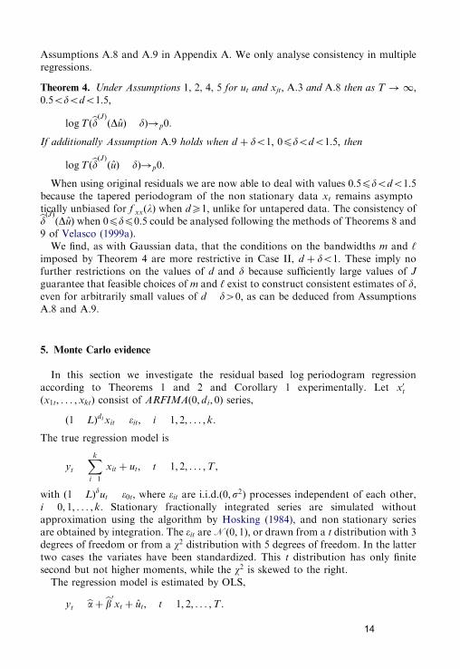
Assumptions A.8 and A.9 in Appendix A. We only analyse consistency in multipleregressions.

Theorem 4. Under Assumptions 1, 2, 4, 5 for ut and xjt; A.3 and A.8 then as T !1;0:5ododo1:5;

logTðbdðJÞðDuÞ dÞ!p0.

If additionally Assumption A.9 holds when d þ do1; 0pdodo1:5; then

logTðbdðJÞðuÞ dÞ!p0.

When using original residuals we are now able to deal with values 0:5pdodo1:5because the tapered periodogram of the non stationary data xt remains asymptotically unbiased for f xxðlÞ when dX1; unlike for untapered data. The consistency ofbdðJÞðDuÞ when 0pdp0:5 could be analysed following the methods of Theorems 8 and9 of Velasco (1999a).

We find, as with Gaussian data, that the conditions on the bandwidths m and ‘imposed by Theorem 4 are more restrictive in Case II, d þ do1: These imply nofurther restrictions on the values of d and d because sufficiently large values of J

guarantee that feasible choices of m and ‘ exist to construct consistent estimates of d;even for arbitrarily small values of d d40; as can be deduced from AssumptionsA.8 and A.9.

5. Monte Carlo evidence

In this section we investigate the residual based log periodogram regressionaccording to Theorems 1 and 2 and Corollary 1 experimentally. Let x0tðx1t; . . . ;xktÞ consist of ARFIMAð0; di; 0Þ series,

ð1 LÞdi xit �it; i 1; 2; . . . ; k.

The true regression model is

yt

Xk

i 1

xit þ ut; t 1; 2; . . . ;T ,

with ð1 LÞdut �0t; where �it are i.i.d.ð0;s2Þ processes independent of each other,i 0; 1; . . . ; k: Stationary fractionally integrated series are simulated withoutapproximation using the algorithm by Hosking (1984), and non stationary seriesare obtained by integration. The �it areNð0; 1Þ; or drawn from a t distribution with 3degrees of freedom or from a w2 distribution with 5 degrees of freedom. In the lattertwo cases the variates have been standardized. This t distribution has only finitesecond but not higher moments, while the w2 is skewed to the right.

The regression model is estimated by OLS,

yt baþ bb0xt þ ut; t 1; 2; . . . ;T .

14

Next, the periodogram is computed from the differenced or original residuals. Thecorresponding log periodogram regressions are

logðI uuðljÞÞ bcþ bdðuÞRj þ vj ; j ‘ þ 1; ‘ þ 2; . . . ;m; lj 2pj=T ,

logðIDuDuðljÞÞ bcþ dd 1ðDuÞRj þ vj ; j ‘ þ 1; ‘ þ 2; . . . ;m,

lj 2pj=ðT 1Þ,

with Rj logð4 sin2ðlj=2ÞÞ � 2 logðljÞ rj : Three different standard errors canbe considered. The usual empirical standard error is given by

1

m ‘

Xm

j ‘þ1

v2j

Xm

j ‘þ1

ðRj R‘Þ2

!�1vuut ; R‘1

m ‘

Xm

j ‘þ1

Rj .

A theoretical modification of the empirical standard errors has been motivatedalready by Geweke and Porter Hudak (1983):

s:e:p2

6

Xm

j ‘þ1

ðRj R‘Þ2

!�1vuut ; R‘1

m ‘

Xm

j ‘þ1

Rj. (7)

Finally, the asymptotic standard error due to Robinson (1995a) is p= 24mp

:Throughout all experiments we found that the theoretical modification given in (7)outperforms the empirical and the asymptotic standard errors in terms of coverageprobabilities. Therefore, only the outcome of t statistics relying on (7) is reported.The test statistics considered hence are

tdbdðuÞ d

s:e:; td

dd 1ðDuÞ þ 1 ds:e:

.

In our experiments the t statistics are compared with standard normal percentiles.Two sided tests at the 1%, 5% and 10% level are applied. We only report results form T0:5; although a more elaborate choice of optimal m has recently been suggestedby Hurvich and Deo (1999) and other deterministic choices such as m T0:4;T0:7

have been tried. These produced similar results, as expected, since given fractionallyintegrated noise models the choice of m should not matter to our main interest, thesize of the test (as long as m is big enough) though power increases with m (and doesnot vary with T). The trimming parameter ‘ is varied very slowly.

Simulations not reported here, in agreement with previous analysis, indicate thatthe normal approximation is valid for true errors irrespective of any trimming ð‘X0Þ;use of nonstationary levels ðd40:5Þ; or leptokurtic t or skewed w2 distributions. OurMonte Carlo design tries to address the validity of these points for residuals and westart investigating how the experimental level of residual based cointegration testsdepends on some of the assumptions that we found sufficient to establish limitingnormality.

15

Tables 1 and 2 report percentages of rejection from 2000 replications when testingfor the true value of d using (differences of) residuals from bivariate regressions with

Gaussian variables. We observe:

(a) Without trimming, ‘ 0; the normal approximation is not valid, at least with the

original residuals without differencing.

(b) Trimming only the first frequency, ‘ 1; provides a satisfactory normal

approximation for T 250 and T 1000 (and also T 500 not reported here).

(c) Even if the gap between d and d is not as big as it should be according to thetheory, i.e. dod 0:5 does not hold, the normal distribution in Tables 1 and 2still yields a useful approximation in case of trimming the first frequency.

Table 1

Experimental level in case of differenced residuals (td), k ¼ 1

d a (%) d ¼ 1:0 d ¼ 0:9 d ¼ 0:8 d ¼ 0:7 d ¼ 0:6 ‘

T ¼ 250; m ¼ 16

1 1.10 1.15 1.45 1.65 2.10

1.4 5 4.70 5.55 5.10 6.00 6.20 0

10 9.75 11.20 10.20 9.85 11.20

1 1.45 1.30 1.15 1.10 1.45

1.4 5 5.65 4.90 5.25 4.95 5.05 1

10 10.50 10.50 10.05 9.85 9.10

1 1.90 1.75 1.60 1.55 1.85

1.0 5 6.50 6.25 5.40 5.60 5.20 0

10 12.15 12.00 10.70 11.15 10.85

1 1.60 2.05 1.30 1.40 1.35

1.0 5 5.15 5.60 5.00 5.10 5.65 1

10 10.00 9.35 8.60 9.25 10.15

T ¼ 1000; m ¼ 32

1 1.80 1.55 1.25 0.85 1.45

1.4 5 6.20 5.75 6.10 5.45 5.30 0

10 10.60 10.80 10.90 10.75 10.35

1 1.10 1.30 1.20 1.30 0.90

1.4 5 4.80 4.90 4.90 4.30 4.70 1

10 10.30 9.30 9.85 8.15 10.45

1 1.50 1.25 1.60 1.85 1.35

1.0 5 5.95 5.50 5.70 6.60 6.55 0

10 10.75 10.55 10.45 11.45 11.75

1 1.20 1.25 1.60 1.10 1.35

1.0 5 5.00 4.80 5.05 4.00 5.60 1

10 9.75 9.50 9.85 9.40 10.00

The variables are integrated of order d while the errors are IðdÞ: All series are constructed from innovations

that follow a Nð0; 1Þ distribution. Tests for the true value of d built upon differenced residuals from

bivariate regressions. Percentage of rejections of two-sided tests at the 1%, 5% and 10% level based on a

standard normal approximation of td: The trimming number is ‘:

16

(d) Even without cointegration, e.g. d d 1 in Tables 1 and 2, the normalapproximation seems to provide a reasonable guideline as long as trimming is

Table 2

Experimental level in case of original residuals (td), k ¼ 1

d a (%) d ¼ 1:0 d ¼ 0:8 d ¼ 0:6 d ¼ 0:4 d ¼ 0:2 ‘

T ¼ 250; m ¼ 16

1 2.85 2.25 2.40 2.25 2.45

1.4 5 8.30 8.10 8.00 7.00 7.25 0

10 15.15 13.70 14.10 11.95 12.10

1 1.80 1.45 1.55 1.40 1.50

1.4 5 5.85 5.55 5.25 5.40 4.90 1

10 9.80 10.05 9.15 9.25 9.25

1 3.15 3.00 2.65 2.20 2.50

1.0 5 8.65 8.35 8.15 7.20 6.85 0

10 14.40 14.15 13.75 12.15 12.25

1 1.55 1.25 1.35 1.20 1.35

1.0 5 4.85 5.90 5.70 5.05 5.60 1

10 9.15 9.30 10.15 9.25 9.30

T ¼ 1000; m ¼ 32

1 2.55 2.60 2.60 2.70 2.65

1.4 5 7.80 7.80 7.05 8.30 7.30 0

10 12.70 13.90 11.60 14.20 12.60

1 1.20 1.40 1.05 1.35 1.45

1.4 5 4.65 5.55 4.80 5.35 5.50 1

10 9.45 10.75 9.40 9.90 10.40

1 2.60 2.00 2.25 2.20 2.00

1.0 5 7.00 7.45 7.40 6.95 6.20 0

10 12.25 12.30 12.25 11.80 10.70

1 1.35 1.55 1.25 1.45 1.40

1.0 5 4.35 6.05 5.65 5.55 5.35 1

10 9.05 11.60 10.65 9.65 10.20

The variables are integrated of order d while the errors are IðdÞ: All series are constructed from innovations

that follow a Nð0; 1Þ distribution. Tests for the true value of d built upon original residuals from bivariate

regressions. Percentage of rejections of two-sided tests at the 1%, 5% and 10% level based on a standard

normal approximation of td: The trimming number is ‘:

applied.

Table 3 considers the power of residual based tests from bivariate regressions andcan be summarized as follows:

(e) As the trimming parameter grows, power decreases.(f) The difference in power between the log periodogram regression of differences or

levels of residuals when testing for d 1 is negligible.

0

(g) From the levels of residuals one may test for d0 0; while tests for this

hypothesis from differences (not reported here) suffer from gross size distortion.

17

Tables 4 and 5 are constructed from residuals from bivariate regressions where2

Table 3

5% power in case of residuals, k ¼ 1

T d0 ¼ 1:0 d1 ¼ 0:9 d1 ¼ 0:8 d1 ¼ 0:7 d1 ¼ 0:6 ‘

Differenced residuals (td¼d0 )250 5.65 6.40 9.50 18.05 26.95 1

ðm ¼ 16Þ 5.35 6.30 8.35 12.80 19.50 2

1000 5.15 8.25 19.70 44.35 67.40 1

ðm ¼ 32Þ 5.55 7.60 15.95 32.25 56.05 2

Original residuals (td¼d0 )

250 5.85 6.35 10.35 17.90 29.35 1

ðm ¼ 16Þ 5.85 5.90 8.30 13.55 20.20 2

1000 4.85 8.30 19.05 43.85 71.05 1

ðm ¼ 32Þ 4.30 7.45 15.40 32.10 57.45 2

Original residuals (td¼d0 )

T d0 ¼ 0:0 d1 ¼ 0:1 d1 ¼ 0:2 d1 ¼ 0:3 d1 ¼ 0:4 ‘250 5.75 6.25 8.85 18.25 28.45 1

ðm ¼ 16Þ 5.00 6.00 9.00 14.45 21.15 2

1000 5.75 8.25 23.90 48.05 71.60 1

ðm ¼ 32Þ 4.35 8.15 17.95 35.05 57.85 2

The regressor is integrated of order 1.4 while the errors are Iðd0Þ under the respective null hypotheses andIðd1Þ under the alternatives. All series are constructed from innovations that follow a Nð0; 1Þ distribution.Tests for d0 built upon differenced or original residuals from bivariate regressions. Percentage of rejections

of two-sided tests at the 5% level based on a standard normal approximation of td or td; respectively. Thetrimming number is ‘:

regressors and errors rely on either t or w distributions (similar results not reportedhere arise for t distributed regressors and w2 distributed residuals and the other wayround). We observe:

(h) The statements (a) (d) continue to hold in case of the considered leptokurtic andskewed distributions.

Next, we investigated the log periodogram regression (of differences) of residualsfrom trivariate regressions, k 2; where all variables are constructed from Gaussian

variates. Again, without trimming the normal approximation is clearly not useful. Furthermore, the following findings arise from Tables 6 and 7.

(i) If d1 d2 1:4; trimming of only the first harmonic frequency, ‘ 1; results in afairly reliable normal approximation. This is also true for the log periodogramregression of residuals without differencing even if d40:5: Moreover, it seems to

hold in case of a cointegration gap smaller than 0.5, e.g. for d 1:

18

(j) If d1 1:4 and d2 0:6; cases I and II are mixed when d 0:2; which violatesAssumption 3. Nevertheless, the normal approximation provides a valid guideline

Table 4

Experimental level in case of differenced residuals (td), k ¼ 1; T ¼ 250

d a (%) d ¼ 1:0 d ¼ 0:9 d ¼ 0:8 d ¼ 0:7 d ¼ 0:6 ‘

t31 2.40 2.00 1.35 2.10 1.70

1.4 5 6.60 6.25 5.35 7.35 7.30 0

10 11.30 11.15 10.20 12.35 12.65

1 0.85 1.15 1.40 0.95 0.85

1.4 5 5.55 5.10 5.30 5.00 4.10 1

10 10.65 9.75 10.45 9.55 9.00

1 2.75 2.30 1.85 2.10 1.65

1.0 5 6.75 7.05 6.15 5.80 5.55 0

10 11.85 11.35 11.35 10.30 10.70

1 1.30 1.25 1.15 1.44 1.40

1.0 5 5.05 5.30 5.05 4.55 4.35 1

10 10.10 9.25 9.45 9.10 9.95

w2ð5Þ1 1.85 1.55 2.40 1.95 1.75

1.4 5 7.25 5.95 6.05 6.25 5.95 0

10 12.20 11.50 11.10 10.60 11.55

1 1.00 0.90 1.40 1.30 1.65

1.4 5 4.25 5.20 5.70 5.25 5.65 1

10 10.05 10.20 10.80 9.80 11.05

1 2.50 2.50 1.95 2.80 1.90

1.0 5 8.00 6.50 6.55 7.40 6.65 0

10 14.05 12.35 11.55 12.85 11.45

1 1.95 1.25 1.35 1.55 1.15

1.0 5 5.00 5.90 5.10 5.30 4.65 1

10 10.40 10.55 10.00 9.85 10.20

The variables are integrated of order d while the errors are IðdÞ: All series are constructed from innovations

that follow either t3 or w2ð5Þ distributions. Tests for the true value of d built upon differenced residuals

from bivariate regressions. Percentage of rejections of two-sided tests at the 1%, 5% and 10% level based

on a standard normal approximation of td: The trimming number is ‘ and m ¼ 16:

in case of trimming the first frequency (original residuals). Surprisingly, this alsoseems to hold for T 250 even if d4d2 0:6; where Assumption 3 is againviolated. For T 1000 observations slightly different results emerge: in case thatd4d2 0:6 trimming only one harmonic frequency is not sufficient for a normalapproximation, so trimming may need to grow with sample size.

We have also investigated in Tables 8 and 9 the effects of pooling a small number J

of periodogram ordinates. In this case the asymptotic variance of the logperiodogram estimate is reduced and we replace in the expression for the standard

19

errors p2=6 by the general expression c0ðJÞ=J for J 1; 2; . . . ; where c is thedigamma function (cf. Robinson, 1995a). Further to the previous findings, we can

Table 5

Experimental level in case of original residuals (td), k ¼ 1; T ¼ 250

d a (%) d ¼ 1:0 d ¼ 0:8 d ¼ 0:6 d ¼ 0:4 d ¼ 0:2 ‘

t31 3.35 3.65 3.30 3.25 2.75

1.4 5 9.50 9.05 9.55 8.50 8.30 0

10 15.30 14.80 16.20 14.15 14.50

1 1.45 1.20 1.20 1.70 1.65

1.4 5 5.25 5.10 4.85 4.80 6.25 1

10 10.20 9.75 9.50 9.00 10.30

1 3.00 2.60 2.25 2.35 2.20

1.0 5 8.35 7.25 7.90 7.10 7.20 0

10 14.10 12.35 14.00 12.80 12.55

1 1.55 0.90 1.60 1.35 1.60

1.0 5 5.80 4.70 4.75 5.35 5.90 1

10 10.05 10.25 10.15 9.90 10.85

w2ð5Þ1 3.45 3.40 2.75 3.30 2.95

1.4 5 10.20 8.25 9.35 10.70 7.45 0

10 15.30 13.95 15.25 17.15 13.10

1 1.25 1.50 1.10 1.15 1.65

1.4 5 4.80 5.05 5.05 5.05 5.80 1

10 9.15 9.25 10.85 10.45 9.60

1 3.55 3.40 2.95 2.65 1.75

1.0 5 9.10 8.65 7.85 7.40 6.50 0

10 14.40 13.70 12.85 12.90 11.15

1 1.30 1.20 1.40 1.10 1.35

1.0 5 4.90 4.75 4.70 4.90 4.90 1

10 9.05 9.95 9.10 9.20 8.85

The variables are integrated of order d while the errors are IðdÞ: All series are constructed from innovations

that follow either t3 or w2ð5Þ distributions. Tests for the true value of d built upon the levels of residuals

from bivariate regressions. Percentage of rejections of two-sided tests at the 1%, 5% and 10% level based

on a standard normal approximation of td: The trimming number is ‘ and m ¼ 16:

state that for Gaussian and other distributions (not reported here),

(k) The larger J, the larger the power with ‘ 1 when testing d0 1 with differencedresiduals or d0 0 with original ones, keeping good size properties.

(l) Use of original residuals with J41 when testing d0 1 requires ‘ 2 tomaintain size, resulting in a noticeable power loss compared to testing based onerrors (Table 8).

This Monte Carlo evidence can be summarized as follows as a rule of thumb forempirical work with bivariate and multiple regressions: If the log periodogram

20

regression is applied to the level of OLS residuals with trimming of the first harmonicfrequency only, then the normal approximation of the t statistic td with theoretical

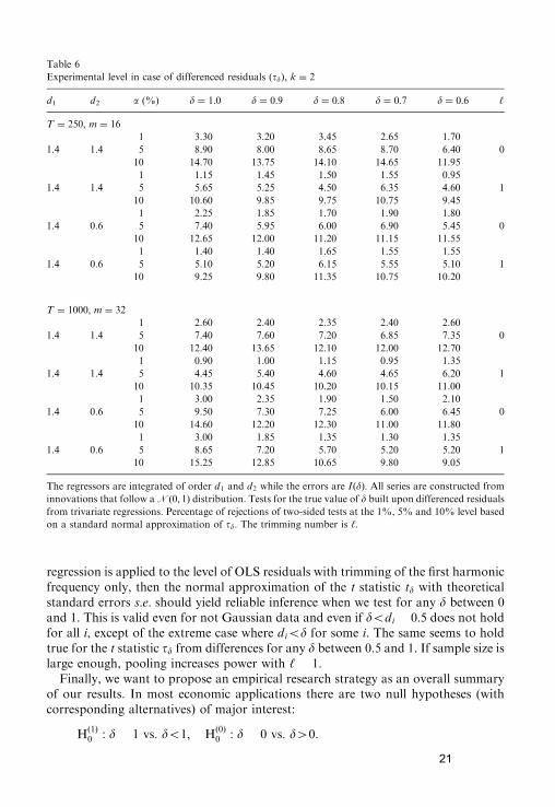
Table 6

Experimental level in case of differenced residuals (td), k ¼ 2

d1 d2 a (%) d ¼ 1:0 d ¼ 0:9 d ¼ 0:8 d ¼ 0:7 d ¼ 0:6 ‘

T ¼ 250; m ¼ 16

1 3.30 3.20 3.45 2.65 1.70

1.4 1.4 5 8.90 8.00 8.65 8.70 6.40 0

10 14.70 13.75 14.10 14.65 11.95

1 1.15 1.45 1.50 1.55 0.95

1.4 1.4 5 5.65 5.25 4.50 6.35 4.60 1

10 10.60 9.85 9.75 10.75 9.45

1 2.25 1.85 1.70 1.90 1.80

1.4 0.6 5 7.40 5.95 6.00 6.90 5.45 0

10 12.65 12.00 11.20 11.15 11.55

1 1.40 1.40 1.65 1.55 1.55

1.4 0.6 5 5.10 5.20 6.15 5.55 5.10 1

10 9.25 9.80 11.35 10.75 10.20

T ¼ 1000; m ¼ 32

1 2.60 2.40 2.35 2.40 2.60

1.4 1.4 5 7.40 7.60 7.20 6.85 7.35 0

10 12.40 13.65 12.10 12.00 12.70

1 0.90 1.00 1.15 0.95 1.35

1.4 1.4 5 4.45 5.40 4.60 4.65 6.20 1

10 10.35 10.45 10.20 10.15 11.00

1 3.00 2.35 1.90 1.50 2.10

1.4 0.6 5 9.50 7.30 7.25 6.00 6.45 0

10 14.60 12.20 12.30 11.00 11.80

1 3.00 1.85 1.35 1.30 1.35

1.4 0.6 5 8.65 7.20 5.70 5.20 5.20 1

10 15.25 12.85 10.65 9.80 9.05

The regressors are integrated of order d1 and d2 while the errors are IðdÞ: All series are constructed from

innovations that follow aNð0; 1Þ distribution. Tests for the true value of d built upon differenced residuals

from trivariate regressions. Percentage of rejections of two-sided tests at the 1%, 5% and 10% level based

on a standard normal approximation of td: The trimming number is ‘:

standard errors s:e: should yield reliable inference when we test for any d between 0and 1. This is valid even for not Gaussian data and even if dodi 0:5 does not holdfor all i, except of the extreme case where diod for some i. The same seems to holdtrue for the t statistic td from differences for any d between 0.5 and 1. If sample size islarge enough, pooling increases power with ‘ 1:Finally, we want to propose an empirical research strategy as an overall summary

of our results. In most economic applications there are two null hypotheses (withcorresponding alternatives) of major interest:

Hð1Þ0 : d 1 vs: do1; H

ð0Þ0 : d 0 vs: d40.

21

We suggest to test Hð1Þ0 from the differences of residuals, while clearly H

ð0Þ0 should be

tested from levels. If, first, both hypotheses are rejected, there is fractional

Table 7

Experimental level in case of original residuals (td), k ¼ 2

d1 d2 a (%) d ¼ 1:0 d ¼ 0:8 d ¼ 0:6 d ¼ 0:4 d ¼ 0:2 ‘

T ¼ 250; m ¼ 16

1 9.35 7.65 5.85 6.50 5.75

1.4 1.4 5 18.80 17.40 16.00 14.90 14.15 0

10 26.80 25.50 23.25 21.60 20.30

1 1.10 1.70 1.60 1.60 1.50

1.4 1.4 5 5.75 5.30 5.05 5.80 5.65 1

10 9.85 10.15 9.70 10.15 9.90

1 4.90 4.35 3.75 5.10 2.65

1.4 0.6 5 12.70 10.70 10.40 11.85 8.40 0

10 19.10 17.35 17.45 16.85 13.85

1 1.60 1.55 2.05 1.90 1.20

1.4 0.6 5 5.90 6.10 6.25 6.40 4.80 1

10 10.50 11.10 10.80 10.80 9.60

T ¼ 1000; m ¼ 32

1 7.45 5.50 5.80 5.30 5.65

1.4 1.4 5 14.05 13.50 13.55 13.45 13.10 0

10 21.95 20.75 20.55 20.85 18.90

1 1.35 1.65 1.95 1.95 0.90

1.4 1.4 5 4.85 5.70 6.80 6.45 4.15 1

10 9.70 11.75 11.55 11.45 9.35

1 5.05 3.65 3.80 3.50 3.05

1.4 0.6 5 13.60 10.10 10.25 8.55 7.55 0

10 20.50 16.15 15.05 14.20 13.35

1 2.85 1.35 1.05 1.60 1.60

1.4 0.6 5 8.70 5.20 4.25 6.30 5.50 1

10 15.10 8.90 8.80 10.65 11.20

The regressors are integrated of order d1 and d2 while the errors are IðdÞ: All series are constructed from

innovations that follow a Nð0; 1Þ distribution. Tests for the true value of d built upon original residuals

from trivariate regressions. Percentage of rejections of two-sided tests at the 1%, 5% and 10% level based

on a standard normal approximation of td: The trimming number is ‘:

cointegration, i.e. we have long memory but transitory equilibrium deviations. Thedegree of persistence d should then be estimated from the levels of the residuals;approximate confidence intervals allow to test whether the estimate is significantlydifferent from 0.5, the borderline of non stationarity. If, second, H

ð0Þ0 is not rejected

while Hð1Þ0 is, we have the strong cointegration result that the errors may be

considered as Ið0Þ: If, third, Hð0Þ0 is rejected while Hð1Þ0 must be accepted, the error

should be considered as Ið1Þ; i.e. persistent, and there is no long run equilibrium. If,finally, none of these hypotheses can be rejected, more data should be used toincrease power.

22

6. Exchange rate dynamics

Table 8

5% power in case of errors with pooling, k ¼ 1

Pooling d0 ¼ 1:0 d1 ¼ 0:9 d1 ¼ 0:8 d1 ¼ 0:7 d1 ¼ 0:6 ‘

Differenced errors (td d0 )

5.10 8.50 17.35 32.15 50.00 0

J ¼ 2 5.05 6.45 11.10 18.55 29.35 1

5.25 6.25 9.10 14.90 23.20 2

5.20 7.60 16.50 29.25 45.40 0

J ¼ 3 5.45 7.25 12.55 21.70 35.55 1

4.70 6.05 8.55 12.10 17.75 2

Original errors (td d0 )

Pooling d0 ¼ 1:0 d1 ¼ 0:9 d1 ¼ 0:8 d1 ¼ 0:7 d1 ¼ 0:6 ‘10.85 7.05 6.85 12.40 24.00 0

J ¼ 2 6.35 5.60 6.95 11.35 20.35 1

4.30 5.15 6.95 10.35 16.55 2

31.45 19.25 9.85 7.75 12.00 0

J ¼ 3 11.80 8.30 7.10 8.95 15.35 1

6.00 5.70 5.50 8.05 10.85 2

Original errors (td d0 )

Pooling d0 ¼ 0:0 d1 ¼ 0:1 d1 ¼ 0:2 d1 ¼ 0:3 d1 ¼ 0:4 ‘5.10 7.30 18.20 37.50 59.65 0

J ¼ 2 5.05 7.20 12.00 22.00 35.25 1

5.25 6.00 9.45 16.00 26.50 2

5.20 6.95 17.75 35.95 59.45 0

J ¼ 3 5.45 6.75 13.30 25.15 39.75 1

4.70 6.00 8.75 13.50 21.70 2

Errors are Iðd0Þ under the respective null hypothesis and Iðd1Þ under the alternatives. All series are

constructed from innovations that follow aNð0; 1Þ distribution. Percentage of rejections of two-sided tests

at the 5% level based on a standard normal approximation of td or td; respectively. Sample size is T ¼ 250:The bandwidth is m ¼ 16: The trimming number is ‘: The pooling number is J.

In a cointegration study with integer orders of integration, Baillie and Bollerslev(1989) argued that seven different nominal spot exchange rates, namely, Germany,the United Kingdom, Japan, Canada, France, Italy and Switzerland, all relative tothe US Dollar and observed daily from 1980 to 1985, do contain unit roots in theirunivariate time series representations, giving also evidence in support of the existenceof a single cointegrating vector between this set of nominal exchange rates. Such acointegration relation has been questioned and found to be fragile by Sephton andLarsen (1991) and Diebold et al. (1994) even though both used the same data set.Diebold et al. note that the lack of cointegration is reinforced when using datacovering the post 1973 floating exchange rate regime. Subsequently, Baillie andBollerslev (1994) collected more reliable evidence in a fractional set up, generalizing

23

the error correction formulation to allow for possible fractional cointegration. Theyfind evidence that a linear combination of the same spot exchange rates contains

Table 9

5% power in case of residuals with pooling, k ¼ 1

Pooling d0 ¼ 1:0 d1 ¼ 0:9 d1 ¼ 0:8 d1 ¼ 0:7 d1 ¼ 0:6 ‘

Differenced residuals (td d0 )

5.20 8.50 16.90 32.05 50.35 0

J ¼ 2 5.55 6.20 10.15 17.75 29.15 1

5.20 6.15 9.10 13.85 23.10 2

5.20 7.25 15.80 29.10 45.20 0

J ¼ 3 5.55 7.05 12.00 21.40 35.10 1

5.50 6.05 8.20 12.30 18.05 2

Original residuals (td d0 )

Pooling d0 ¼ 1:0 d1 ¼ 0:9 d1 ¼ 0:8 d1 ¼ 0:7 d1 ¼ 0:6 ‘9.65 8.55 13.95 25.80 42.05 0

J ¼ 2 6.70 5.80 7.75 12.50 21.55 1

5.60 5.50 6.45 10.80 17.35 2

21.30 11.80 8.25 13.15 23.10 0

J ¼ 3 13.15 7.55 6.65 9.80 16.65 1

7.05 5.65 5.60 7.45 10.50 2

Original residuals (td d0 )

Pooling d0 ¼ 0:0 d1 ¼ 0:1 d1 ¼ 0:2 d1 ¼ 0:3 d1 ¼ 0:4 ‘6.90 6.25 12.20 25.10 45.35 0

J ¼ 2 5.10 6.55 11.40 19.80 31.10 1

5.15 5.40 9.20 15.10 25.00 2

6.80 6.50 12.25 24.90 44.40 0

J ¼ 3 5.65 6.20 11.85 22.25 37.30 1

4.75 5.70 8.05 13.00 21.60 2

The regressors are integrated of order 1.4 while the errors are Iðd0Þ under the respective null hypothesis

and Iðd1Þ under the alternatives. All series are constructed from innovations that follow a Nð0; 1Þdistribution. Tests for d0 built upon original residuals from bivariate regressions. Percentage of rejections

of two-sided tests at the 5% level based on a standard normal approximation of td or td; respectively.Sample size is T ¼ 250: The bandwidth is m ¼ 16: The trimming number is ‘: The pooling number is J.

long range dependence. In particular, they estimate an error correction term withmemory 0.89 in a fractional white noise model, with an (asymptotic) standard errorof 0.02.

In this section we confirm their results for the same seven currencies. We usemonthly data taken from Citibase and run from 1974.1 until 1997.12, which leaves uswith T 288 observations. Following Baillie and Bollerslev (1994), the logarithmsof the data are analysed. The use of monthly observations may help to controlchanging conditional variances and should not affect the analysis of long runproperties compared to higher frequency data.

24

Table 10

Correlogram of CAN

First First

Levels differences Levels differences

Lag ACF PACF

1 0.988 0.204 0.988 0.204

2 0.975 0.019 0.041 0.063

3 0.963 0.015 0.024 0.034

4 0.951 0.056 0.023 0.046

5 0.937 0.047 0.074 0.071

6 0.923 0.024 0.019 0.056

7 0.910 0.010 0.027 0.015

8 0.895 0.193 0.017 0.207

9 0.879 0.107 0.081 0.028

10 0.863 0.229 0.025 0.233

Correlogram and partial correlogram for the Canada exchange rate. The asymptotic standard error is

0.117 under the null of no correlation.

On application of the well known ADF test to our data set, we obtain p valuesgreater than 0.05. Moreover, in some cases we cannot reject the presence of a unitroot at any conventional significance level. For example, in the Canadian case, thevalue obtained of the ADF test is 0.63, whereas the 10% critical value is 2.87. Tofurther confirm this claim, in Table 10 we present the ACF and PACF of the levelsand first differences of the Canada exchange rate series. It can be observed that theautocorrelations exhibit the typical very slow decline associated with a nonstationaryprocess, and that the autocorrelations of the change, i.e. the autocorrelations of theapproximate rate of return, are all them small.

Nonetheless, an alternative potential explanation for the high persistence of theexchange rate is the possibility that the memory parameters of these series may befractional, since it is well known that standard integer order unit root tests have lowpower against fractional alternatives (cf., e.g., Hassler and Walter, 1994; Dolado andMarmol, 1997).

In order to confirm this possibility, we start with determining the memory of theindividual series by applying the log periodogram regression without trimming, ‘0; to the differences of the original data. The regression range was chosen as m

18; 20; 22: This choice provided fairly stable estimates and avoids the first seasonalfrequency, which given our monthly data is lT=12 l24: However these bandwidthsare far from mean square optimal choices, T4=5 � 93; which would lead to seriousbias in semiparametric estimates and distortions in our statistical inference.

With the standard errors s:e: from (7), the estimates presented in Table 11 forGermany, UK, Switzerland and Japan are not significantly different from 1, whileFrance, Italy and Canada have significantly larger values. Consequently, if we testaccording to Robinson (1995a) that all seven estimates are equal, the p value of the

25

Wald statistics are always less than 0.001. Note that this multivariate inference isonly valid under no cointegration (cf. Assumption A.2). The null hypothesis that

Table 11

Individual memory, 1974.1 1997.12

GER UK SWI JAP FRA ITA CAN

m ¼ 18 bdðDuÞ 1.17 1.02 0.86 1.24 1.41 1.34 1.40

td¼1 0.88 0.10 0.72 1.23 2.11 1.75 2.06

m ¼ 20 bdðDuÞ 1.15 1.10 0.84 1.23 1.33 1.34 1.44

td¼1 0.81 0.53 0.88 1.29 1.84 1.86 2.42

m ¼ 22 bdðDuÞ 1.18 1.15 0.84 1.16 1.31 1.32 1.35

td¼1 1.07 0.88 0.93 0.94 1.80 1.90 2.05

Log-periodogram regression of differences of logarithms with ‘ ¼ 0: The t statistics built on the standard

errors s:e: ¼ 0:194; 0:181; 0:170 for m ¼ 18; 20; 22; respectively.

Table 12

Residual analysis for separate regressions

m 17 18 19 20 21 22

s:e: 0.262 0.250 0.240 0.230 0.221 0.213

FRA on ITA, CANbdðDuÞ 1.37 1.23 1.18 1.14 1.05 0.99

td¼1 1.41 0.92 0.75 0.61 0.23 0.05

GER on UK, SWI, JAPbdðDuÞ 0.79 0.74 0.88 0.89 0.84 0.92

td¼1 0.80 1.04 0.50 0.48 0.72 0.38

Log-periodogram regression of differenced residuals with ‘ ¼ 1: The t statistics built on the standard error

s:e: from (7).

France, Italy and Canada have the same memory parameter, however, is clearly notrejected (p value 40:964), while the hypothesis of a common d of Germany, UK,Switzerland and Japan is not rejected at the 5% level for small m. We conclude thatthere are two groups of data: Germany, UK, Switzerland and Japan may beconsidered as Ið1Þ; while the order of integration of France, Italy and Canada isroughly 1.4.

We hence start with separate cointegrating regressions and apply the logperiodogram regression to differenced residuals. First, France is regressed on Italyand Canada, see the upper panel in Table 12. With trimming the first frequency,‘ 1; and varying m we clearly cannot reject that the residuals are integrated of

26

Table 13

Final residual analysis

GER on UK, SWI, JAP and RES(FRA on ITA, CAN)

m 17 18 19 20 21 22

From differences, H0 : d ¼ 1bdðDuÞ 0.46 0.49 0.62 0.67 0.65 0.66

td 1 2.06 2.04 1.58 1.44 1.58 1.60

p-val. 0.020 0.021 0.057 0.075 0.057 0.055

From levels, H0 : d ¼ 0bdðuÞ 0.63 0.61 0.67 0.69 0.66 0.68

td 0 2.41 2.44 2.79 3.00 2.99 3.19

p-val. 0.008 0.007 0.003 0.001 0.001 0.001

Log-periodogram regression of differenced and original residuals with ‘ ¼ 1: The t statistics built on the

standard error s:e: from Table 12.

order one. Hence, we have three Ið1:4Þ series that cointegrate to Ið1Þ residuals. In thelower panel of Table 12 it is reported that the null hypothesis that the Ið1Þ series fromGermany, UK, Switzerland and Japan do not cointegrate ðd 1Þ; cannot berejected.

Finally, we regress the German data on UK, Switzerland, Japan and the Ið1Þresidual RES from the regression of France on Italy and Canada. The results withtrimming one frequency are presented in Table 13. From differences we first test thenull of no cointegration, d 1: For all m from 17 to 22 it is rejected at least at the10% level, and most of the times the p values are close or below the 5% level. At thesame time, the log periodogram regression of the original residuals clearly rejects thenull hypothesis d 0: We conclude that it is fractional cointegration that links theconsidered exchange rates. The memory parameter d of the equilibrium deviations isestimated as approximately 0.65 from levels as well as from differences. It is neversignificantly different from 0.5, i.e. we cannot not reject that the error term is nonstationary, although we have found that it is not persistent ðdo1Þ:

We also did the analysis from Table 13 without trimming, ‘ 0: The resulting t

statistics not reported here are very similar to those from Table 13, because thestandard errors are smaller without trimming and the estimates are closer to the null.From levels one roughly estimates bdðuÞ 0:5; while the log periodogram regressionfrom differences yields approximately bdðDuÞ 0:7: The findings with trimming fromTable 13 where bdðuÞ � bdðDuÞ seem to be more reliable.

7. Concluding remarks

In this paper we followed the route opened by Robinson (1995a, Remark 7) for

sound statistical inference on memory properties of fractional models. He suggestedthat given a sufficiently fast rate of convergence of the regression estimator the

27

residual based log periodogram regression should result in asymptotic normality justas with observed series (confer the application in Robinson and Marinucci, 2001).Indeed, we found that given the gap between the orders of integration of regressorsand error is big enough, the log periodogram regression of residuals gives rise tolimiting normality. This result essentially relies on trimming the very first fewfrequencies of the periodogram, a policy that was not employed by the empirical andexperimental papers reviewed in the introduction. We hence obtained simpleconditions for consistent estimation of the degree of persistence in the deviationsfrom the long run equilibrium which are more general than most parametric modelsused in common practice. Given asymptotically normal estimators this allows forstatistical inference of immediate economic interest. We are now able to discriminateon sound asymptotic grounds between short memory errors, stationary longmemory innovations, non stationary but transitory equilibrium deviations, andfinally non stationary and persistent errors.

Our results also cover the integer cointegration case of Ið1Þ regressors with Ið0Þerrors. But contrasting the residual based work by Phillips and Ouliaris (1990), Shin(1994) or more recently Xiao (1999) the asymptotic theory we suggest is standardand moreover does not depend on the number of regressors. What is more, a systemapproach of joint estimation of the orders of integration of regressors anddisturbance term is possible, and a pooled version was shown to be robust todepartures from Gaussianity and from strongly cointegrated systems with d

d40:5: We evaluated the asymptotic results by means of Monte Carlo experimentswhere it turned out that trimming only one frequency should be enough for practicalpurposes with usual sample sizes.

To illustrate these points we applied the log periodogram regression to a set ofseven nominal exchange rates, collecting evidence that exchange rates are linked by afractional cointegration relation. In this respect, with our semiparametric set up weconclude that there could be two clusters of currencies. On the one hand, Germany,UK, Switzerland and Japan, that may be considered as Ið1Þ processes. On the otherhand, France, Italy and Canada, with an order of integration about 1.4. We fail tofind evidence of cointegration among the first group of exchange rates, whereas wecannot reject that the residuals from a regression of France on Italy and Canada areIð1Þ: However, we find polynomial cointegration when regressing the German dataon UK, Switzerland, Japan and the residuals from the regression of France on Italyand Canada, so that they do not drift apart in the long run. The memory parameterof the equilibrium deviations of this extended regression is about 0.65, i.e. the errorcorrection term is non stationary but not persistent.

Acknowledgements

We are grateful to P.M. Robinson and two referees, and to the participants at the8th World Congress of the Econometric Society, Seattle, 2000, and at the Workshopon New Approaches to the Study of Economic Fluctuations by CEPR, Hydra, 2000,for very helpful comments on an earlier version. This paper was completed while the

28

first author was visiting Universidad Carlos III de Madrid. Financial supportthrough the European Commission programme Training and Mobility of Researchers

and CICYT Refs. No. SEC 2001 08090 and BEC 2001 1270 and SEJ 2004 04583/

ECON is gratefully acknowledged.

Appendix A. Assumptions and auxiliary results

For our asymptotic theory we will need to impose the following regularityassumption (cf. Assumptions 1 and 2 of Robinson, 1995a) which applies either to thespectral density (of stationary processes) or to the pseudospectral density (of nonstationary processes), imposing the rate in (1).

Assumption A.1. The (pseudo) spectral density f zzðlÞ of zt; z 2 fx; ug(dx d; du d) satisfies, 0ogp2; 0oGzo1;

f zzðlÞ Gzl�2dz ð1þOðjljgÞÞ as l! 0,

and is differentiable in a neighbourhood ð0; �Þ of the origin with

d

dlf zzðlÞ

���� ���� Oðjlj�1�2dz Þ as l! 0.

This assumption holds for standard ARFIMA series with g 2 and for anyfractional model with f ðlÞ ð2 sinðl=2ÞÞ�2dz f �ðlÞ; if in an interval of the origin eitherthe Ið0Þ short memory spectral density f �ðlÞ is LipschitzðgÞ; 0ogp1; or its derivativeis Lipschitz ðg 1Þ; 1ogp2: The following assumption is a multivariate generalization of this set up for zt containing possibly both stationary and non stationaryelements (cf. Robinson, 1995a).

Assumption A.2. The (pseudo) spectral density matrix fðlÞ ðf ijðlÞÞ of zt

ðDdut;Dx0tÞ0 satisfies, 0ogp2; 0oGio1; i; j 0; 1; . . . ; k;

f iiðlÞ Gil�2Di ð1þOðjljgÞÞ as l! 0,

where d bdþ 0:5c and Do d d; and is differentiable in a neighbourhood ð0; �Þof the origin with

d

dlf ijðlÞ

���� ���� Oðjlj�1�Di�Dj Þ as l! 0.

Set the coherence matrix RðlÞ of ðDdut;Dx0tÞ0; with typical element RijðlÞ

f ijðlÞ=ðf iiðlÞf jjðlÞÞ1=2; the coherence between zit and zjt: Then Rð0Þ is not singular

and for some a 2 ð0; 2�;

jRijðlÞ Rijð0Þj OðjljaÞ as l! 0.

For tapered periodograms we impose the following assumption strengtheningAssumption A.1, and which holds, for e.g. ARFIMA models with g 2; and relaxesconditions such as f zzðlÞjlj

2d2 Gz þ Egjljg þ oðjljgÞ; as l! 0; 0oEgo1 used inVelasco (2000).

29

Assumption A.3. Let ut possess a (pseudo) spectral density f uuðlÞ satisfyingAssumption A.1 such that for jojpl=2 and some 1ogp2

f uuðl oÞ f uuðlÞ of 0uuðlÞ þOðjlj�2d�gjojgÞ as l! 0.

The following are restrictions on the bandwidths defined in Assumption 2.

Assumption A.4. maxf0; ð1 d dÞ=ðd d 0:5Þgoboao1; d d40:5:

Assumption A.5. 0oboao2g=ð1þ 2gÞ:

Note that depending on the values of d; d and g; these two assumptions may nothold simultaneously. Thus, for example, if g 2; like for ARFIMA processes, weneed 9d þ d47; because of ð1 d dÞ=ðd d 0:5Þo4=5; which holds for any dX0if d4 7

9:However, we always require d40:75 for Assumption A.4 to hold, because of

ð1 d dÞ=ðd d 0:5Þo1:

Assumption A.6. 0oboao2minfa; gg=ð1þ 2minfa; ggÞ:

Assumption A.7. maxf0; ð1 di dÞ=ðdi d 0:5Þgoboao1; min di d40:5:

Assumption A.8. 0oboao2Jbðd dÞ; gJ=ðJ þ 2Þ41; JX3:

Assumption A.9. When d þ do1; 0oboao2Jfbðd dÞ ð1 d dÞg:

The following theorem is the main result on log periodogram regressions withobserved data.

Theorem A.1. Under Assumption A.1, for Gaussian ut�IðdÞ; 0:5odo0:5; ‘ 0 and

m�1ðlogTÞ2 þ T�2gm1þ2g! 0 as T !1, (8)

then

m1=2ðbdðuÞ dÞ!dN 0;p2

24

� �.

Proof of Theorem A.1. It follows from Robinson (1995a), using Hurvich et al. (1998)techniques to show that trimming of very low frequencies is not necessary for theasymptotic normality of bd: Though Hurvich et al. (1998) only consider fractionalprocesses with Ið0Þ innovations which possess a spectral density f �ðlÞ with threebounded derivatives around l 0; their results are easily generalized to our set upwith 0ogp2 in Assumption A.1. Note that they also used the asymptoticallyequivalent regressor logð4 sin2ðlj=2ÞÞ proposed by Geweke and Porter Hudak(1983) which arises naturally for fractional processes. &

The condition T�2gm1þ2g! 0 as T !1 in (8) reflects the fact that when thesemiparametric model Gul

�2d is not very appropriate for high frequencies, i.e. g issmall in Assumption A.1, m must not grow very fast to avoid higher frequency biasesin the local regression. The logT consistency holds under weaker conditions onbandwidth numbers, as is shown by estimating the mean square error of bdðuÞ as inHurvich et al. (1998).

30

Theorem A.2. Under Assumption A.1, for Gaussian ut; 0:5odo0:5; ‘ 0 and

ðm�1 þ ðT�1mÞ2gÞðlogTÞ2 þ T�1m logm! 0 as T !1, (9)

then logTðbdðuÞ dÞ!p0:

In many cases we may wish to exclude the first ‘40 frequencies in the regressionand both asymptotic normality and logT consistency hold as shown originally byRobinson (1995a):

Corollary A.1. Theorems A.1 and A.2 hold if m�1‘ðlogTÞ2 ! 0 as T !1:

Now follows the general result for multivariate log periodogram regressions.

Theorem A.3. Under Assumption A.2 for Gaussian ðut;Dx0tÞ0; 0:5od; d 1o0:5; and

m�1ðlogTÞ2 þ T�2minfa;ggm1þ2minfa;gg ! 0 as T !1, (10)

we obtain that

2m1=2ðbdðuÞ dÞ!dNð0;OÞ.

This holds if trimming is introduced as long as ‘m�1ðlogTÞ2! 0 as T !1: The

covariance matrix O can be estimated consistently by the sample regression residuals

covariance matrix, bO ðm ‘Þ�1Pm

j ‘þ1 ej e0j :

Proof of Theorem 7. This follows from Robinson (1995a), extendingto a multivariate set up the results by Hurvich et al. (1998) to avoid trimming,‘ 0: &

The following theorem is the basic result for non Gaussian log periodogramregressions.

Theorem A.4. Under Assumptions 4, 5, A.1, A.3, 0:5pdo1:5; gJ=ðJ þ 2Þ41; JX3;and

‘�1 þm�1‘ðlogTÞ2 þ T�1m! 0 as T !1, (11)

then bdðJÞðuÞ!pd:

Proof of Theorem A.4. This follows directly using the methods of Velasco (2000) for0odo0:5: The extension to 0:5odo0 and 0:5pdo1:5 being immediate (cf.Velasco, 2000, Lemma 3, 1999a, Theorems 4 and A.1). &

We collect in two lemmas several results repeatedly used in our proofs furtherdown.

Lemma A.1. Under Assumption A.1, 0:5ododo1:5; ‘�1 þmT�1 ! 0 as T !1;z 2 fx; ug ðdx d; du dÞ; j ‘ þ 1; . . . ;m;

E½IDzDzðljÞ� f DzDzðljÞð1þOðj�1 logðj þ 1ÞÞÞ Oðl2�2dzj Þ, (12)

31

and if zt is Gaussian,

max‘þ1pjpm

E½ðIDzDzðljÞ=f DzDzðljÞÞa�o1; a4 1, (13)

max‘þ1pjpm

IDzDzðljÞ=f DzDzðljÞ OpðlogTÞ. (14)

Proof of Lemma A.1. Eq. (12) follows from Robinson (1995a), Theorem 2. For a40;(13) follows from Gaussianity and (12). For 1oao0; (13) follows fromGaussianity and the proof of Lemma 5 of Hurvich et al. (1998). They used a

1=4: Finally (14) can be proved using Gaussianity, (13) and adapting the proofs ofTheorems 4.5.1. and 5.3.2. of Brillinger (1975). &

Lemma A.2. Under Assumption A.1, 0pdodo1:5; ‘�1 þm�1T ! 0 as T !1;z 2 fx; ug (dx d; du d) j ‘ þ 1; . . . ;m; some Ko1;

E½IzzðljÞ=f zzðljÞ�1þOðj�1 log j þ j2ðdz�1Þ logðj þ 1ÞÞ; dzo1;

pKj2ðdz�1Þ; 1pdzo1:5;

(and if zt is Gaussian,

max‘þ1pjpm

E½ðIzzðljÞ=f zzðljÞÞa�o1; a4 1; dzo1;

max‘þ1pjpm

IzzðljÞ=f zzðljÞ OpðlogTÞ; dzo1;

max‘þ1pjpm

IzzðljÞj2ð1�dzÞ=f zzðljÞ OpðlogTÞ; 1pdzo1:5. (15)

Proof of Lemma A.2. It can be proved along the same lines as Lemma A.1,using now Velasco (1999a) and Hurvich and Ray (1995, Theorem 1) fornon stationary series to bound E½IzzðljÞ=f zzðljÞ�: The remaining results follow fromGaussianity. &

Appendix B. Proofs

Proof of Theorem 1. All sums run for j ‘ þ 1; . . . ;m if not indicated otherwise.First we obtain from (4) that

!�1 bdðDuÞ bdðDuÞ

Xj

W 2j

Xm

j ‘þ1

W j logIDuDuðljÞ

IDuDuðljÞ, (16)

where W j is defined in (5). Note that (8), (9) and the condition on the trimminghold under the conditions of the theorem with the definition of m and ‘;so it only remains to show that the effects of the residual approximation arenegligible to deduce the asymptotic properties of bdðDuÞ from those of bdðDuÞ:

32

We can write from Eq. (3) that

logIDuDuðljÞ

IDuDuðljÞlog 1 ðbb bÞ

wDxðljÞ

wDuðljÞ

� �þ log 1 ðbb bÞ

wDxð ljÞ

wDuð ljÞ

� �, (17)

so

max‘þ1pjpm

ðbb bÞwDxðljÞ

wDuðljÞ

���� ����pjbb bj max‘þ1pjpm

wDxðljÞ

f DxDxðljÞp�����

����� max‘þ1pjpm

f DxDxðljÞp

wDuðljÞ

����������.

Since d þ dX1 (Case I), from Lemma A.1 above,

jbb bj max‘þ1pjpm

wDxðljÞ

f DxDxðljÞp�����

����� OpðTd�d logTp

Þ, (18)

and for any c40 fixed and 0o�o1; using Bonferroni’s and Markov’sinequalities and (13) in Lemma A.1 with a ð�=2Þ 14 1 and z x; andAssumption A.1,

P Td�d log2 T max‘þ1pjpm

f DxDxðljÞp

wDuðljÞ

����������4c

( )

pXm

j ‘þ1

P Td�d log2 Tf DxDxðljÞ

pwDuðljÞ

����������4c

( )

OXm

j ‘þ1

E Td�d log2 Tf DxDxðljÞ

IDuDuðljÞ

s" #2��0@ 1AO log4 T

Xm

j ‘þ1

j�ðd�dÞð2��Þ

!Oð‘1�ðd�dÞð2��Þ log4 TÞ oð1Þ,

using Assumption 2, since d d4a4 12

for some a and choosing� 2 ð1=aÞ40 so

max‘þ1pjpm

f DxDxðljÞp

wDuðljÞ

���������� opðT

d�d log�2 TÞ. (19)

Therefore from (18) and (19)

max‘þ1pjpm

ðbb bÞwDxðljÞ

wDuðljÞ

���� ���� opðlog�1 TÞ. (20)

33

Then, using (17) and j logð1þ xÞjp2jxj for jxjp 12; and the indicator function I;

Xm

j ‘þ1

W j logIDuDuðljÞ

IDuDuðljÞ

����������

pXm

j ‘þ1

jW jj logIDuDuðljÞ

IDuDuðljÞ

���� ����I ðbb bÞwDxðljÞ

wDuðljÞ

���� ����p 1

2

� �

þXm

j ‘þ1

jW jj logIDuDuðljÞ

IDuDuðljÞ

���� ����I ðbb bÞwDxðljÞ

wDuðljÞ

���� ����4 1

2

� �

p4jbb bj max‘þ1pjpm

jW jjXm

j ‘þ1

wDxðljÞ

wDuðljÞ

���� ����þ max

‘þ1pjpmlog

IDuDuðljÞ

IDuDuðljÞ

���� ���� max‘þ1pjpm

jW jjXm

j ‘þ1

I ðbb bÞwDxðljÞ

wDuðljÞ

���� ����4 1

2

� �

Now, d d40:5;

jbb bj max‘þ1pjpm

jW jjXm

j ‘þ1

wDxðljÞ

wDuðljÞ

���� ���� Op logTXm

j ‘þ1

jd�d

!opðm

1=2Þ,

because jbb bj OpðTd�dÞ; (Case I), max‘þ1pjpmjW jj OðlogTÞ (noting definition

(5) of W t), Assumption 2, so using (12) of Lemma A.1 and applying Holder’sinequality with 1opo2; 1=qþ 1=p 1Þ;

EwDxðljÞ

wDuðljÞ

���� ����pCld�dj E

wDxðljÞ

f DxDxðljÞp�����

�����q !1=q

Ef DuDuðljÞ

pwDuðljÞ

����������p !1=p

O ld�dj

.

(21)

On the other hand, we obtain that

max‘þ1pjpm

logIDuDuðljÞ

IDuDuðljÞ

���� ���� opðlog�1 TÞ,

using (17) and because (20) implies that for any c40;

P logT maxj

log 1 ðbb bÞwDxðljÞ

wDuðljÞ

� ����� ����4c

� �pP logT max

jðbb bÞ

wDxðljÞ

wDuðljÞ

���� ����4c=2

� �oð1Þ,

since j logð1þ xÞj4c= logT implies jxj4c=ð2 logTÞ for all c40 and T large enough.

34

Finally,Xm

j ‘þ1

I ðbb bÞwDxðljÞ

wDuðljÞ

���� ����4 1

2

� �p2jbb bj

Xm

j ‘þ1

wDxðljÞ

wDuðljÞ

���� ����Op

Xm

j ‘þ1

jd�d

!opðm

1=2 log�1 TÞ,

using (21), Assumption 2 and d d40:5: The theorem follows from (16),4Pm

j ‘þ1 W 2j�m and because under Assumption A.5, (8) holds and therefore

Theorem A.1 gives the result since the residual contribution is opðm�1=2Þ: &

Proof of Theorem 2. First we write

bdðuÞ bdðuÞ Xj

W 2j

!�1Xj

W j logI uuðljÞ

IuuðljÞ. (22)

Next, from Robinson (1995a), and adapting the argument of Hurvich et al. (1998),since (9) holds, ðbdðuÞ dÞ logT!p0: Also (8) holds when ao2g=ð1þ 2gÞ; m1=2ðbdðuÞdÞ!dNð0;p2=24Þ: Then it only remains to be shown that the right hand side of (22) isnegligible.

Case I : When d þ dX1 and do1; we can proceed exactly as in Theorem 1, usingLemma A.2 instead of Lemma A.1, so

Xj

W 2j

!�1 Xm

j ‘þ1

W j logI uuðljÞ

IuuðljÞOp m�1 logT

Xm

j ‘þ1

jd�d

!opðm

�1=2Þ,

because d d40:5:When dX1; E½IxxðljÞ=f xxðljÞ� is no longer bounded as T !1 and we have to

proceed differently. Let us show that

max‘þ1pjpm

ðbb bÞwxðljÞ

wuðljÞ

���� ����pjbb bj max‘þ1pjpm

wxðljÞ

f xxðljÞp j1�d

���������� max‘þ1pjpm

f xxðljÞp

wuðljÞjd�1

����������

opðlog�1 TÞ.

Using Lemma A.2, dX1;

jbb bj max‘þ1pjpm

wxðljÞ

f xxðljÞp j1�d

���������� OpðT

d�d logTp

Þ,

and for any c40 fixed and 0o�o1; using Bonferroni’s and Markov’s inequalitiesand Lemma A.2, as in the proof of Theorem 1,

P Td�d log2 T max‘þ1pjpm

f xxðljÞp

wuðljÞjd�1

����������4c

( )

pXm

j ‘þ1

P Td�d jd�1log2 Tf xxðljÞ

pwuðljÞ

����������4c

( )

35

OXm

j ‘þ1

E Td�d jd�1 log2 Tf xxðljÞ

IuuðljÞ

s" #2��0@ 1AO log4 T

Xm

j ‘þ1

j�ð1�dÞð2��Þ

!Oð‘1�ð1�dÞð2��Þ log4 TÞ oð1Þ,

using Assumption 2 since do0:5 implies that for some a, 1 d4a40:5 and choosing� 2 ð1=aÞ40; so, dX1;

max‘þ1pjpm

f xxðljÞp

wuðljÞjd�1

���������� opðT

d�d log�2 TÞ.

Now, do0:5;

jbb bj max‘þ1pjpm

jW jjXm

j ‘þ1

wxðljÞ

wuðljÞ

���� ���� Op logTXm

j ‘þ1

jd�1

!opðm

1=2Þ,

because jbb bj OpðTd�dÞ; max‘þ1pjpmjW jj OðlogTÞ; and because using Lem

ma A.2, (1opo2; q�1 þ p�1 1), we obtain now for dX1

EwxðljÞ

wuðljÞ

���� ����pCld�dj jd�1 E

wxðljÞ

f xxðljÞp j1�d

����������q !1=q

Ef uuðljÞ

pwuðljÞ

����������p !1=p

Oðld�dj jd�1Þ.

On the other hand, max‘þ1pjpmj log I uuðljÞ=IuuðljÞj opðlog�1 TÞ as in Theorem 1,

so it only remains to bound

Xm

j ‘þ1

I ðbb bÞwxðljÞ

wuðljÞ

���� ����4 1

2

� �p2jbb bj

Xm

j ‘þ1

wxðljÞ

wuðljÞ

���� ���� ¼ Op

Xm

j ‘þ1

jd 1

!¼ opðm

1=2 log 1 TÞ,

using the definition of m and do0:5:Case II : If d þ do1 then do1; and we obtain first that,

max‘þ1pjpm

ðbb bÞwxðljÞ

wuðljÞ

���� ���� opðlog�1 TÞ,

because jbb bj OpðT1�2dÞ and for any c40; using Lemma A.2,

P T1�2d log2 T max‘þ1pjpm

f xxðljÞp

wuðljÞ

����������4c

( )

OXm

j ‘þ1

E T1�2d log2 Tf xxðljÞ

IuuðljÞ

s" #2��0@ 1A36

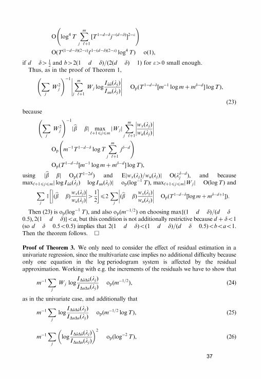
O log4 TXm

j ‘þ1

½T1�d�dj�ðd�dÞ�2��

!OðT ð1�d�dÞð2��Þ‘1�ðd�dÞð2��Þ log4 TÞ oð1Þ,

if d d4 12and b42ð1 d dÞ=ð2ðd dÞ 1Þ for �40 small enough.

Thus, as in the proof of Theorem 1,

Xj

W 2j

!�1 Xm

j ‘þ1

W j logI uuðljÞ

IuuðljÞ

���������� OpðT

1�d�d½m�1 logmþmd�d � logTÞ,

(23)

because

Xj

W 2j

!�1jbb bj max

‘þ1pjpmjW jj

Xm

j ‘þ1

wxðljÞ

wuðljÞ

���� ����Op m�1T1�d�d logT

Xm

j ‘þ1

jd�d

!OpðT

1�d�d½m�1 logmþmd�d � logTÞ,

using jbb bj OpðT1�2dÞ and EjwxðljÞ=wuðljÞj Oðld�d

j Þ; and becausemax‘þ1pjpmj log I uuðljÞ log IuuðljÞj opðlog

�1 TÞ; max‘þ1pjpmjW jj OðlogTÞ andXj

I ðbb bÞwxðljÞ

wuðljÞ

���� ����4 1

2

� �p2

Xj

ðbb bÞwxðljÞ

wuðljÞ

���� ���� OpðT1�d�d½logmþmd�dþ1�Þ.

Then (23) is opðlog�1 TÞ; and also opðm

�1=2Þ on choosing maxfð1 d dÞ=ðd d0:5Þ; 2ð1 d dÞgoa; but this condition is not additionally restrictive because d þ do1(so d d 0:5o0:5) implies that 2ð1 d dÞoð1 d dÞ=ðd d 0:5Þoboao1:Then the theorem follows. &

Proof of Theorem 3. We only need to consider the effect of residual estimation in aunivariate regression, since the multivariate case implies no additional difficulty becauseonly one equation in the log periodogram system is affected by the residualapproximation. Working with e.g. the increments of the residuals we have to show that

m�1X

j

W j logIDuDuðljÞ

IDuDuðljÞopðm

�1=2Þ, (24)

as in the univariate case, and additionally that

m�1X

j

logIDuDuðljÞ

IDuDuðljÞopðm

�1=2 logTÞ, (25)

m�1X

j

logIDuDuðljÞ

IDuDuðljÞ

� �2

opðlog�2 TÞ, (26)

37

from (5.6), (5.8) and (5.13) in Robinson (1995a) for consistent covariance matrixestimation. Now to show (24) we can write now that

logIDuDuðljÞ

IDuDuðljÞlog 1

Xk

i 1

ðbbi biÞwDxiðljÞ

wDuðljÞ

( )

þ log 1Xk

i 1

ðbbi biÞwDxið ljÞ

wDuð ljÞ

( ).

Next,

max‘þ1pjpm

Xk

i 1

ðbbi biÞwDxiðljÞ

wDuðljÞ

����������

pXk

i 1

jbbi bijmaxj

wDxiðljÞ

f DxiDxiðljÞ

p����������max

j

f DxiDxiðljÞ

pwDuðljÞ

����������

opðlog�1 TÞ, ð27Þ

since k is finite, bounding the above expression for each i 1; . . . ; k as in the univariatecase. Then (25) follows in a similar but simpler way, while (26) is implied directly by(27). &

Proof of Theorem 4. For simplicity, we suppress in the notation for IuuðljÞ; etc.reference to J or tapering and only consider the case of a univariate regressor xt:Weconsider successively the cases of differenced and original residuals.

Proof for differenced residuals. We obtain that dd 1ðJÞðDuÞ dd 1

ðJÞðDuÞ

opðlog�1 TÞ if we show that

max‘þ1pjpm

jW jj logIDuDuðljÞ

IDuDuðljÞopðlog

�1 TÞ,

which in turn follows if

max‘þ1pjpm

ðbb bÞwDxðljÞ

wDuðljÞ

���� ����pjbb bj max‘þ1pjpm

wDxðljÞ

f DxDxðljÞp�����

����� max‘þ1pjpm

f DxDxðljÞp

wDuðljÞ

����������

opðlog�2 TÞ. ð28Þ

We first show that

jbb bj max‘þ1pjpm

wDxðljÞ

f DxDxðljÞp�����

����� OpðTd�d logTp

Þ. (29)

We have jbb bj OpðTd�dÞ while, writing I �DxDxðljÞ for the periodogram

of the i.i.d. innovations �ðDxÞt of zt Dxt in Assumption 4, and HDxDxðljÞ

38

IDxDxðljÞf�1DxDxðljÞ 2pI �DxDxðljÞ;

max‘þ1pjpm

wDxðljÞ

f DxDxðljÞp�����

����� !2

p max‘þ1pjpm

2pI �DxDxðljÞ þ max‘þ1pjpm

jHDxDxðljÞj

p max‘þ1pjpm

2pI �DxDxðljÞ þXm

j ‘þ1

jHDxDxðljÞj2

!1=2

.

Now, max‘þ1pjpm 2pI �DxDxðljÞ OpðlogTÞ; see An et al. (1983), while from Velasco(2000), 1ogp2;

EXm

j ‘þ1

IDxDxðljÞ

f DxDxðljÞ2pI �DxDxðljÞ

���� ����2 OXm

j ‘þ1

j�g

!Oð‘1�gÞ,

so (29) follows. Then (28) follows if we show that

max‘þ1pjpm

f DxDxðljÞp

wDuðljÞ

���������� OpðT

d�d log�3 TÞ.

For any sequence MT ! 0 as T !1; and with C40; 0oto1 fixed,0:5ododo1:5; HDuDuðljÞ IDuDuðljÞf

�1DuDuðljÞ 2pI �DuDuðljÞ; now using the innova

tions of Dut; we have that

P MT

f DuDuðljÞ

IDuDuðljÞ4C

� �P 2pI �DuDuðljÞ 1þ

HDuDuðljÞ

2pI �DuDuðljÞ

� �oC�1MT

� �pP 2pI �DuDuðljÞoðC�1MT Þ

t� �þ P 1þ

HDuDuðljÞ

2pI �DuDuðljÞ

� �oðC�1MT Þ

1�t� �

pP 2pI �DuDuðljÞoðC�1MT Þt� �þ P

HDuDuðljÞ

2pI �DuDuðljÞ

���� ����4 1

2

� �OðMJ�v

T þ j�a�1Þ, ð30Þ

for any v40; on choosing to1 large enough, and some a such that 0oaoðgJ=ðJ þ2Þ 1Þ=2; following Eqs. (A.8) and (A.13) in Velasco (2000).

Set MT ‘2ðd�dÞ log3 T oð1Þ as T !1 by Assumption A.8.Then we can writefor any C40 and some v;C040; using (30),

P Td�d log2 T maxj

f DxDxðljÞp

wDuðljÞ

����������4C

( )pP MT max

j

f DuDuðljÞ

IDuDuðljÞ4C0

� �

39

pX

j

P MT

f DuDuðljÞ

IDuDuðljÞ4C0

� �

OX

j

½MJ�vT þ j�a�1�

!Oðm‘2ðd�dÞðJ�vÞ log3J

þ ‘�aÞ oð1Þ

choosing v40 small enough and using Assumption A.8.

Proof for original residuals. We want to show that bdðJÞðuÞ bdðJÞðuÞ opðlog�1 TÞ:

Case I : When d þ dX1 and do1:5; we can proceed exactly as for Du; but now weobtain that

jbb bj max‘þ1pjpm

wxðljÞ

f xxðljÞp�����

����� OpðTd�d logTp

Þ,

because from Velasco (1999b) (see also Lemmas 1 and 3 of Lobato and Velasco,2000) and for tapered data, 0:5odo1:5; 1ogp2;

EXm

j ‘þ1

IxxðljÞ

f xxðljÞ2pI �DxDxðljÞ

���� ����2 OXm

j ‘þ1

j�g

!Oð‘1�gÞ.

Then we can write as before, for any C; v40; MT ‘2ðd�dÞ log3 T oð1Þ as T !

1; and using now the innovations of ut if do0:5; or those of Dut if dX0:5;

P Td�d log3 T maxj

f xxðljÞp

wuðljÞ

����������4C

( )OX

j

maxj½MJ�v

T þ j�a�1�

!þ oð1Þ

Oðm‘2ðd�dÞðJ�vÞ log3J T þ ‘�aÞ þ oð1Þ

oð1Þ,

with Assumption A.8, so finally

maxj

f xxðljÞp

wuðljÞ

���������� opðT

d�dÞ.

Case II : If d þ do1 then do1; do0:5; and we proceed as before toshow that

max‘þ1pjpm

ðbb bÞwxðljÞ

wuðljÞ

���� ���� opðlog�2 TÞ.

Using Assumption 1 we first obtain that

jbb bj max‘þ1pjpm

wxðljÞ

f xxðljÞp�����

����� OpðT1�2d log1=2 TÞ.

40

Then we show that

max‘þ1pjpm

f xxðljÞp

wuðljÞ

���������� opðT

2d�1 log�3 TÞ,

because with the same notation, MT T2ð1�d�dÞ‘2ðd�dÞ log3 T oð1Þ by AssumptionA.9,

P T1�2d log2 T maxj

f xxðljÞp

wuðljÞ

����������4C

( )pP MT max

j

f uuðljÞ

IuuðljÞ4C0

� �OðmMJ�v

T þ ‘�aÞ þ oð1Þ,

which is OðmfT2ð1�d�dÞ‘2ðd�dÞ log6 TgJ�vÞ þ oð1Þ oð1Þ; using Assumptions A.8 andA.9. &

References

An, H.-Z., Chen, Z.-G., Hannan, E.J., 1983. The maximum of the periodogram. Journal of Multivariate

Analysis 13, 383 400.

Baillie, R.T., 1996. Long memory processes and fractional integration in econometrics. Journal of

Econometrics 73, 5 59.

Baillie, R.T., Bollerslev, T., 1989. Common stochastic trends in a system of exchange rates. The Journal of

Finance 44, 167 181.

Baillie, R.T., Bollerslev, T., 1994. Cointegration, fractional cointegration, and exchange rate dynamics.

The Journal of Finance 49, 737 745.

Booth, G.G., Tse, Y., 1995. Long memory in interest rate future markets: a fractional cointegration

analysis. The Journal of Future Markets 15, 573 584.

Breitung, J., Hassler, U., 2002. Inference on the cointegration rank in fractionally integrated processes.

Journal of Econometrics 110, 167 185.

Brillinger, D.R., 1975. Time Series. Data Analysis and Theory. Holden Day, San Francisco.

Chen, Z.-G., Hannan, E.J., 1980. The distribution of periodogram ordinates. Journal of Time Series

Analysis 1, 73 82.

Cheung, Y.-E., Lai, K.S., 1993. A fractional cointegration analysis of purchasing power parity. Journal of

Business and Economic Statistics 11, 103 122.

Dahlhaus, R., 1989. Efficient parameter estimation for self-similar processes. Annals of Statistics 14,

517 532.

De Jong, R.M., Davidson, J., 2000. The functional central limit theorem and convergence to stochastic

integrals II: the fractionally integrated case. Econometric Theory 16, 643 666.

Diebold, F.X., Gardeazabal, J., Yilmaz, K., 1994. On cointegration and exchange rate dynamics. The

Journal of Finance 49, 727 735.

Dolado, J.J., Marmol, F., 1997. On the properties of the Dickey Pantula test against fractional

alternatives. Economics Letters 57, 11 16.

Dueker, M., Startz, R., 1998. Maximum-likelihood estimation of fractional cointegration with an

application to U.S. and Canadian bond rates. The Review of Economics and Statistics 80, 420 426.

Engle, R.F., Granger, C.W.J., 1987. Co-integration and error correction: representation, estimation and

testing. Econometrica 55, 251 276.

Fay, G., Soulier, P., 2001. The periodogram of an i.i.d. sequence. Stochastic Processes and Their

Applications 92, 315 343.

41

Fox, R., Taqqu, M.S., 1986. Large-sample properties of parameter estimates for strongly dependent

stationary Gaussian times series. Annals of Statistics 14, 517 532.

Geweke, J., Porter-Hudak, S., 1983. The estimation and application of long memory time series models.

Journal of Time Series Analysis 4, 221 238.

Gil-Alana, L.A., Robinson, P.M., 1997. Testing of unit root and other non-stationary hypotheses in

macroeconomic time series. Journal of Econometrics 80, 241 268.

Granger, C.W.J., 1981. Some properties of time series data and their in econometric model specification.

Journal of Econometrics 16, 121 130.

Granger, C.W.J., Joyeux, R., 1980. An introduction to long memory time series models and fractional

differencing. Journal of Time Series Analysis 1, 15 39.

Hassler, U., Walter, J., 1994. On the power of unit root tests against fractional alternatives. Economics

Letters 45, 1 5.

Hosking, J.R.M., 1981. Fractional differencing. Biometrika 68, 165 176.

Hosking, J.R.M., 1984. Modeling persistence in hydrological time series using fractional differencing.

Water Resources Research 20, 1898 1908.

Hurvich, C.M., Deo, R., 1999. Plug-in selection of the number of frequencies in regression estimates

of the memory parameter of a long-memory time series. Journal of Time Series Analysis 20,

331 341.

Hurvich, C.M., Ray, B.K., 1995. Estimation of the memory parameter for nonstationary or noninvertible

fractionally integrated processes. Journal of Time Series Analysis 16, 17 42.

Hurvich, C.M., Deo, R., Brodsky, J., 1998. The mean square error of Geweke and Porter Hudak’s

estimator of the memory parameter of a long memory time series. Journal of Time Series Analysis 19,

19 46.

Kim, C., Phillips, P.C.B., 2001. Fully modified estimation of fractional cointegration models. Preprint,

Yale University.

Kunsch, H.R., 1987. Statistical aspects of self-similar processes. Proceedings 1st World Congress of the

Bernoulli Society, VNU Science Press, pp. 67 74.

Lobato, I.N., Velasco, C., 2000. Long memory in stock market trading volume. Journal of Economic and

Business Statistics 18, 410 427.

Marinucci, D., Robinson, P.M., 1999. Alternative forms of fractional Brownian motion. Journal of

Statistical Planning and Inference 80, 111 122.

Masih, R., Masih, A.M.M., 1995. A fractional cointegration approach to empirical tests of PPP: new

evidence and methodological implications from an application to the Taiwan/US dollar relationship.

Review of World Economics 131, 673 694.

Masih, A.M.M., Masih, R., 1998. A fractional cointegration approach to testing mean reversion between

spot and forward exchange rates: a case of high frequency data with low frequency dynamics. Journal

of Business Finance and Accounting 25, 987 1003.

Phillips, P.C.B., Ouliaris, S., 1990. Asymptotic properties of residual based tests for cointegration.

Econometrica 58, 165 193.

Robinson, P.M., 1994a. Time series with strong dependence. In: Sims, C.A. (Ed.), Advances in

Econometrics. Sixth World Congress, vol. I. Cambridge University Press, Cambridge, pp. 47 95.

Robinson, P.M., 1994b. Semiparametric analysis of long-memory time series. Annals of Statistics 22,

515 539.

Robinson, P.M., 1995a. Log-periodogram regression of time series with long range dependence. Annals of

Statistics 23, 1048 1072.

Robinson, P.M., 1995b. Gaussian semiparametric estimation of long range dependence. Annals of

Statistics 23, 1630 1661.

Robinson, P.M., 1997. Large sample inference for nonparametric regression with dependent errors.

Annals of Statistics 25, 2054 2083.

Robinson, P.M., Marinucci, D., 2000. The averaged periodogram for nonstationary vector time series.

Statistical Inference for Stochastic Processes 3, 149 160.

Robinson, P.M., Marinucci, D., 2001. Narrow-band analysis of nonstationary processes. Annals of

Statistics 29, 947 986.

42

R

S

S

S

S

T

V

V

V

X

obinson, P.M., Yajima, Y., 2002. Determination of cointegration rank in fractional systems. Journal of

Econometrics 106, 217–241.

ephton, P.S., Larsen, H.K., 1991. Tests of exchange market efficiency: fragile evidence from cointegration

tests. Journal of International Money and Finance 10, 561–570.

hin, Y., 1994. A residual-based test of the null of cointegration against the alternative of no

cointegration. Econometric Theory 10, 91–115.

oofi, A.S., 1998. A fractional cointegration test of purchasing power parity: the case of selected members

of OPEC. Applied Financial Economics 8, 559–566.

owell, F.B., 1992. Maximum likelihood estimation of stationary univariate fractionally integrated time

series. Journal of Econometrics 53, 165–188.

se, Y.K., Anh, V.V., Tieng, A., 1999. No-cointegration test based on fractional differencing: Some

Monte Carlo results. Journal of Statistical Planning and Inference 80, 257–267.

elasco, C., 1999a. Non-stationary log-periodogram regression. Journal of Econometrics 91, 325–371.

elasco, C., 1999b. Gaussian semiparametric estimation of non-stationary time series. Journal of Time

Series Analysis 20, 87–127.

ARTICLE IN PRESS

U. Hassler et al. / Journal of Econometrics 130 (2006) 165–207 207

elasco, C., 2000. Non-Gaussian log-periodogram regression. Econometric Theory 16, 44–79.

iao, Z., 1999. A residual based test for the null hypothesis of cointegration. Economics Letters 64,

133–141.

43