APPROXIMATION METHODS

Kenneth L. Judd

Hoover Institution

July 19, 2011

1

Approximation Methods

• General Objective: Given data about f(x) construct simpler g(x) approximating f(x).

• Questions:

— What data should be produced and used?

— What family of “simpler” functions should be used?

— What notion of approximation do we use?

• Comparisons with statistical regression

— Both approximate an unknown function and use a finite amount of data

— Statistical data is noisy but we assume data errors are small

— Nature produces data for statistical analysis but we produce the data in function approximation

2

Interpolation Methods

• Interpolation: find g (x) from an n-dimensional family of functions to exactly fit n data points

• Lagrange polynomial interpolation

— Data: (xi, yi) , i = 1, .., n.

— Objective: Find a polynomial of degree n− 1, pn(x), which agrees with the data, i.e.,

yi = f(xi), i = 1, .., n

— Result: If the xi are distinct, there is a unique interpolating polynomial

3

• Does pn(x) converge to f (x) as we use more points?

— No! Consider

f(x)=1

1 + x2xi=−5,−4, ..., 3, 4, 5

Figure 1:

— Why does this fail? because there are zero degrees of freedom? bad choice of points? bad

function?

4

• Hermite polynomial interpolation

— Data: (xi, yi, y′

i) , i = 1, .., n.

— Objective: Find a polynomial of degree 2n− 1, p(x), which agrees with the data, i.e.,

yi=p(xi), i = 1, .., n

y′i=p′(xi), i = 1, .., n

— Result: If the xi are distinct, there is a unique interpolating polynomial

• Least squares approximation

— Data: A function, f(x).

— Objective: Find a function g(x) from a class G that best approximates f(x), i.e.,

g = argming∈G

‖f − g‖2

5

Orthogonal polynomials

• General orthogonal polynomials

— Space: polynomials over domain D

— Weighting function: w(x) > 0

— Inner product: 〈f, g〉 =∫D f(x)g(x)w(x)dx

— Definition: {φi} is a family of orthogonal polynomials w.r.t w (x) iff⟨φi, φj

⟩= 0, i �= j

— We can compute orthogonal polynomials using recurrence formulas

φ0(x)=1

φ1(x)=x

φk+1(x)=(ak+1x+ bk)φk(x) + ck+1φk−1(x)

6

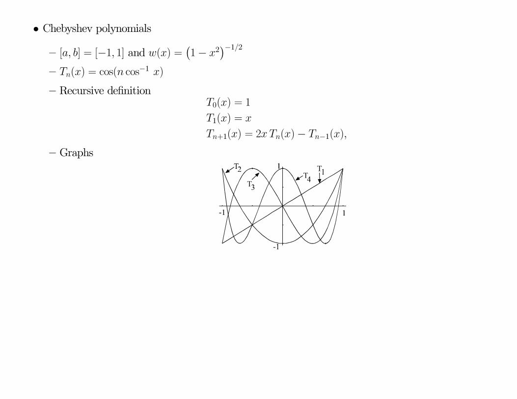
• Chebyshev polynomials

— [a, b] = [−1, 1] and w(x) =(1− x2

)−1/2

— Tn(x) = cos(n cos−1 x)

— Recursive definitionT0(x) = 1

T1(x) = x

Tn+1(x) = 2xTn(x)− Tn−1(x),

— Graphs

7

• General intervals

— Few problems have the specific intervals and weights used in definitions

— One must adapt the polynomials to fit the domain through linear COV:

∗ Define the linear change of variables that maps the compact interval [a, b] to [−1, 1]

y = −1 + 2x− a

b− a

∗ The polynomials φ∗

i (x) ≡ φi

(−1 + 2x−a

b−a

)are orthogonal over x ∈ [a, b] with respect to the

weight w∗ (x) ≡(−1 + 2x−a

b−a

)iff the φi (y) are orthogonal over y ∈ [−1, 1] w.r.t. w (y)

8

Regression

• Data: (xi, yi) , i = 1, .., n.

• Objective: Find a function f(x;β) with β ∈ Rm, m ≤ n, with yi.= f(xi), i = 1, .., n.

• Least Squares regression:

minβ∈Rm

∑(yi − f (xi;β))

2

9

Algorithm 6.4: Chebyshev Approximation Algorithm in R1

• Objective: Given f(x) defined on [a, b], find its Chebyshev polynomial approximation p(x)

• Step 1: Compute the m ≥ n+ 1 Chebyshev interpolation nodes on [−1, 1]:

zk = −cos

(2k − 1

2mπ

), k = 1, · · · ,m.

• Step 2: Adjust nodes to [a, b] interval:

xk = (zk + 1)

(b− a

2

)+ a, k = 1, ...,m.

• Step 3: Evaluate f at approximation nodes:

wk = f(xk) , k = 1, · · · ,m.

• Step 4: Compute Chebyshev coefficients, ai, i = 0, · · · , n :

ai =

∑mk=1wkTi(zk)∑mk=1 Ti(zk)2

to arrive at approximation of f(x, y) on [a, b]:

p(x) =n∑i=0

aiTi

(2x− a

b− a− 1

)

10

Minmax Approximation

• Data: (xi, yi) , i = 1, .., n.

• Objective: L∞ fit

minβ∈Rm

maxi

‖yi − f (xi;β)‖

• Problem: Difficult to compute

• Chebyshev minmax property

Theorem 1 Suppose f : [−1, 1] → R is Ck for some k ≥ 1, and let In be the degree n polynomial

interpolation of f based at the zeroes of Tn+1(x). Then

‖ f − In ‖∞≤

(2

πlog(n+ 1) + 1

)

×(n− k)!

n!

(π2

)k(b− a

2

)k

‖ f (k) ‖∞

• Chebyshev interpolation:

— converges in L∞; essentially achieves minmax approximation

— works even for C2 and C3 functions

— easy to compute

— does not necessarily approximate f ′ well

11

Splines

Definition 2 A function s(x) on [a, b] is a spline of order n iff

1. s is Cn−2 on [a, b], and

2. there is a grid of points (called nodes) a = x0 < x1 < · · · < xm = b such that s(x) is a polynomial

of degree n− 1 on each subinterval [xi, xi+1], i = 0, . . . ,m− 1.

Note: an order 2 spline is the piecewise linear interpolant.

• Cubic Splines

— Lagrange data set: {(xi, yi) | i = 0, · · · , n}.

— Nodes: The xi are the nodes of the spline

— Functional form: s(x) = ai + bi x+ ci x2 + di x

3 on [xi−1, xi]

— Unknowns: 4n unknown coefficients, ai, bi, ci, di, i = 1, · · ·n.

12

• Conditions:

— 2n interpolation and continuity conditions:

yi =ai + bixi + cix2i + dix

3i ,

i = 1, ., n

yi =ai+1 + bi+1xi + ci+1x2i + di+1x

3i ,

i = 0, ., n− 1

— 2n− 2 conditions from C2 at the interior: for i = 1, · · ·n− 1,

bi + 2cixi + 3dix2i =bi+1 + 2ci+1 xi + 3di+1x

2i

2ci + 6dixi=2ci+1 + 6di+1xi

— Equations (1—4) are 4n− 2 linear equations in 4n unknown parameters, a, b, c, and d.

— construct 2 side conditions:

∗ natural spline: s′′(x0) = 0 = s′′(xn); it minimizes total curvature,∫ xnx0

s′′(x)2 dx, among

solutions to (1-4).

∗ Hermite spline: s′(x0) = y′0 and s′(xn) = y′n (assumes extra data)

∗ Secant Hermite spline: s′(x0) = (s(x1)−s(x0))/(x1−x0) and s′(xn) = (s(xn)−s(xn−1))/(xn−

xn−1).

∗ not-a-knot: choose j = i1, i2, such that i1 + 1 < i2, and set dj = dj+1, j = i1, i2.

— Solve system by special (sparse) methods; see spline fit packages

13

Shape Issues

• Approximation methods and shape

— Concave (monotone) data may lead to nonconcave (nonmonotone) approximations.

— Example

— Shape problems destabilize value function iteration

14

• Schumaker Procedure:

1. Take level (and maybe slope) data at nodes xi

2. Add intermediate nodes z+i ∈ [xi, xi+1]

3. Run quadratic spline with nodes at the x and z nodes which intepolate data and preserves

shape.

4. Schumaker formulas tell one how to choose the z and spline coefficients (see book and correction

at book’s website)

15

• Shape-preserving orthogonal polynomial approximation

— Let Least squares Chebyshev approximation preserving increasing concave shape with Lagrange

data (xi, vi)

mincj

m∑i=1

⎛⎝ n∑

j=0

cjφj (xi)− vi

⎞⎠

2

s.t.n∑

j=1

cjφ′

j (xi) > 0,

n∑j=1

cjφ′′

j (xi) < 0, i = 1, . . . ,m.

— Least squares Chebyshev approximation preserving increasing concave shape withHermite data

(xi, vi, v′

i)

mincj

m∑i=1

⎛⎝ n∑

j=0

cjφj (xi)− vi

⎞⎠

2

+ λm∑i=1

⎛⎝ n∑

j=0

cjφ′

j (xi)− v′i

⎞⎠

2

s.t.n∑

j=1

cjφ′

j (xi) > 0, i = 1, . . . ,m,

n∑j=1

cjφ′′

j (xi) < 0, i = 1, . . . ,m.

where λ is some parameter.

16

• L1 Shape-preserving approximation

— L1 increasing concave approximation

mincj

m∑i=1

∣∣∣∣∣∣n∑

j=1

cjφj (xi)− vi

∣∣∣∣∣∣s.t.

n∑j=1

cjφ′

j (zk) ≥ 0, k = 1, . . . ,K

n∑j=1

cjφ′′

j (zk) ≤ 0, k = 1, . . . ,K

— NOTE: We impose shape on a set of points, zk, possibly different, and generally larger, from

the approximation points, xi.

17

— This looks like a nondifferentiable problem, but it is not when we rewrite it as

mincj,λi

m∑i=1

λi

s.t.n∑

j=1

cjφ′

j (zk) ≥ 0, k = 1, . . . ,K

n∑j=1

cjφ′′

j (zk) ≤ 0, k = 1, . . . ,K

−λi≤n∑

j=1

cjφj (xi)− vi ≤ λi, i = 1, . . . ,m

0≤λi, i = 1, . . . ,m

18

• Use possibly different points for shape constraints; generally you want more shape checking points

than data points.

• Mathematical justification: semi-infinite programming

• Many other procedures exist for one-dimensional problems, but few procedures exist for two-

dimensional problems

19

Multidimensional approximation methods

• Lagrange Interpolation

— Data: D ≡ {(xi, zi)}Ni=1 ⊂ Rn+m, where xi ∈ Rn and zi ∈ Rm

— Objective: find f : Rn → Rm such that zi = f(xi).

— Need to choose nodes carefully.

— Task: Find combinations of interpolation nodes and spanning functions to produce a nonsin-

gular (well-conditioned) interpolation matrix.

20

Tensor products

• General Approach:

— If A and B are sets of functions over x ∈ Rn, y ∈ Rm, their tensor product is

A⊗B = {ϕ(x)ψ(y) | ϕ ∈ A, ψ ∈ B}.

— Given a basis for functions of xi, Φi = {ϕi

k(xi)}∞

k=0, the n-fold tensor product basis for functions

of (x1, x2, . . . , xn) is

Φ =

{n∏i=1

ϕiki(xi) | ki = 0, 1, · · · , i = 1, . . . , n

}

• Orthogonal polynomials and Least-square approximation

— Suppose Φi are orthogonal with respect to wi(xi) over [ai, bi]

— Least squares approximation of f(x1, · · · , xn) in Φ is∑ϕ∈Φ

〈ϕ, f〉

〈ϕ, ϕ〉ϕ,

where the product weighting function

W (x1, x2, · · · , xn) =n∏i=1

wi(xi)

defines 〈·, ·〉 over D =∏

i[ai, bi] in

〈f(x), g(x)〉 =

∫D

f(x)g(x)W (x)dx.

21

Algorithm 6.4: Chebyshev Approximation Algorithm in R2

• Objective: Given f(x, y) defined on [a, b] × [c, d], find its Chebyshev polynomial approximation

p(x, y)

• Step 1: Compute the m ≥ n+ 1 Chebyshev interpolation nodes on [−1, 1]:

zk = −cos

(2k − 1

2mπ

), k = 1, · · · ,m.

• Step 2: Adjust nodes to [a, b] and [c, d] intervals:

xk = (zk + 1)

(b− a

2

)+ a, k = 1, ...,m.

yk = (zk + 1)

(d− c

2

)+ c, k = 1, ...,m.

• Step 3: Evaluate f at approximation nodes:

wk,� = f(xk, y�) , k = 1, · · · ,m. , � = 1, · · · ,m.

• Step 4: Compute Chebyshev coefficients, aij, i, j = 0, · · · , n :

aij =

∑mk=1

∑m�=1wk,�Ti(zk)Tj(z�)

(∑m

k=1 Ti(zk)2) (∑m

�=1 Tj(z�)2)

to arrive at approximation of f(x, y) on [a, b]× [c, d]:

p(x, y) =n∑i=0

n∑j=0

aijTi

(2x− a

b− a− 1

)Tj

(2y − c

d− c− 1

)

22

Complete polynomials

• Taylor’s theorem for Rn produces the approximation

f(x).=f(x0) +

∑ni=1

∂f∂xi

(x0) (xi − x0i )

+12

∑ni1=1

∑ni2=1

∂2f∂xi1∂xik

(x0)(xi1 − x0i1)(xik − x0ik) + ...

— For k = 1, Taylor’s theorem for n dimensions used the linear functionsPn1 ≡ {1, x1, x2, · · · , xn}

— For k = 2, Taylor’s theorem uses Pn2 ≡ Pn

1 ∪ {x21, · · · , x2n, x1x2, x1x3, · · · , xn−1xn}.

• In general, the kth degree expansion uses the complete set of polynomials of total degree k in n

variables.

Pnk ≡ {xi11 · · ·xinn |

n∑�=1

i� ≤ k, 0 ≤ i1, · · · , in}

• Complete orthogonal basis includes only terms with total degree k or less.

• Sizes of alternative bases

degree k Pnk Tensor Prod.

2 1 + n+ n(n+ 1)/2 3n

3 1 + n+ n(n+1)2 + n2 + n(n−1)(n−2)

6 4n

— Complete polynomial bases contains fewer elements than tensor products.

— Asymptotically, complete polynomial bases are as good as tensor products.

— For smooth n-dimensional functions, complete polynomials are more efficient approximations

23

• Construction

— Compute tensor product approximation, as in Algorithm 6.4

— Drop terms not in complete polynomial basis (or, just compute coefficients for polynomials in

complete basis).

— Complete polynomial version is faster to compute since it involves fewer terms

— Almost as accurate as tensor product; in general, degree k + 1 complete is better then degree

k tensor product but uses far fewer terms.

24

Shape Issues

• Much harder in higher dimensions

• No general method

• The L2 and L1 methods generalize to higher dimensions.

— The constraints will be restrictions on directional derivatives in many directions

— There will be many constraints

— But, these will be linear constraints

— L1 reduces to linear programming; we can now solve huge LP problems, so don’t worry.

25