GEOL 452/552 - GIS for Geoscientists I

Lecture 22 - Chapter 8 (Raster Analysis, part 3)

• More on raster functions: - Interpolation (Inverse Distance based, IDW)- Zonal Analysis (statistics) for polygons, lines, points- Effects Toolbar

• more: Geol 488/588 - GIS II (rasters, TIN, ArcScene), Spr. 2013

• Iowa Ortho image server and USGS Seamless raster data server

• Suitability Analysis HowTo (possible class project idea?)

1

• copy geol552/data/follow along/Ch8C_more_data

• into your U:\ArcGIS\Ch8A_class_ex folder

• start mxd file in U:\ArcGIS\Ch8A_class_ex

• ArcMap: add layers from Ch8C_more_data to your data frame

• Activate Spatial Analyst

• Geoprocessing - Environments:

• Workspace: U:\ArcGIS\Ch8a_class_ex

• set Extent to extent of dem.img

2

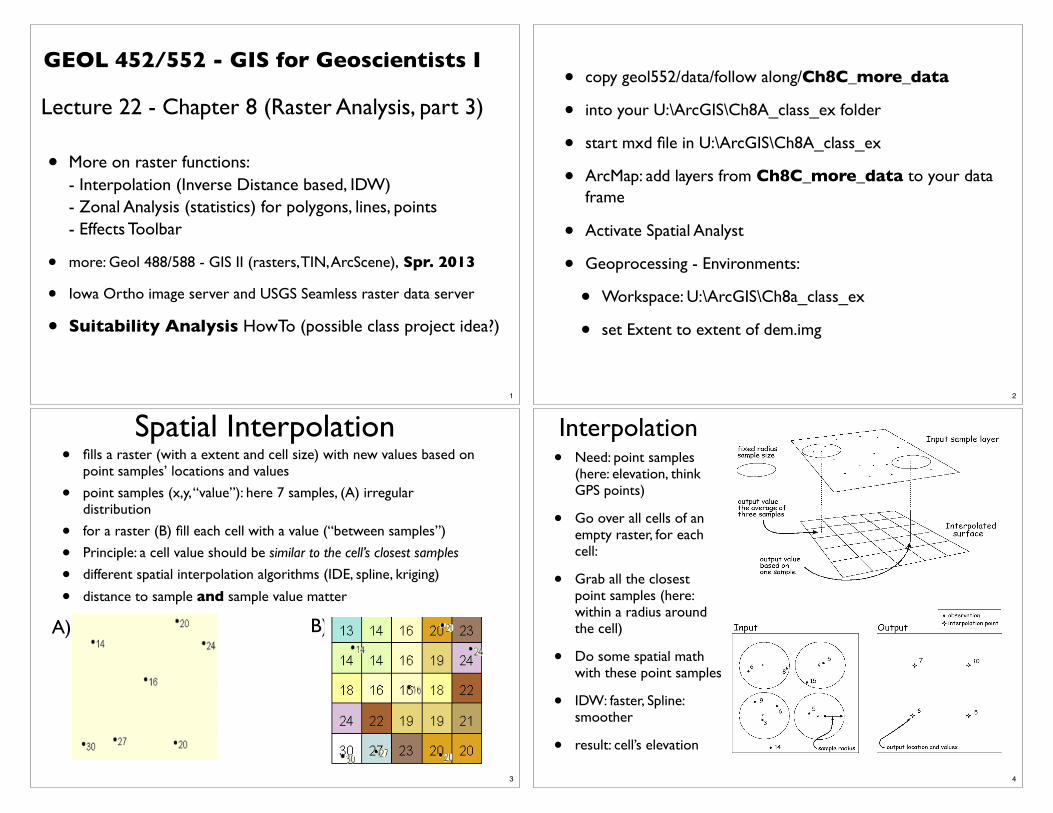
Spatial Interpolation• fills a raster (with a extent and cell size) with new values based on

point samples’ locations and values

• point samples (x,y, “value”): here 7 samples, (A) irregular distribution

• for a raster (B) fill each cell with a value (“between samples”)

• Principle: a cell value should be similar to the cell’s closest samples

• different spatial interpolation algorithms (IDE, spline, kriging)

• distance to sample and sample value matter

A) B)

3

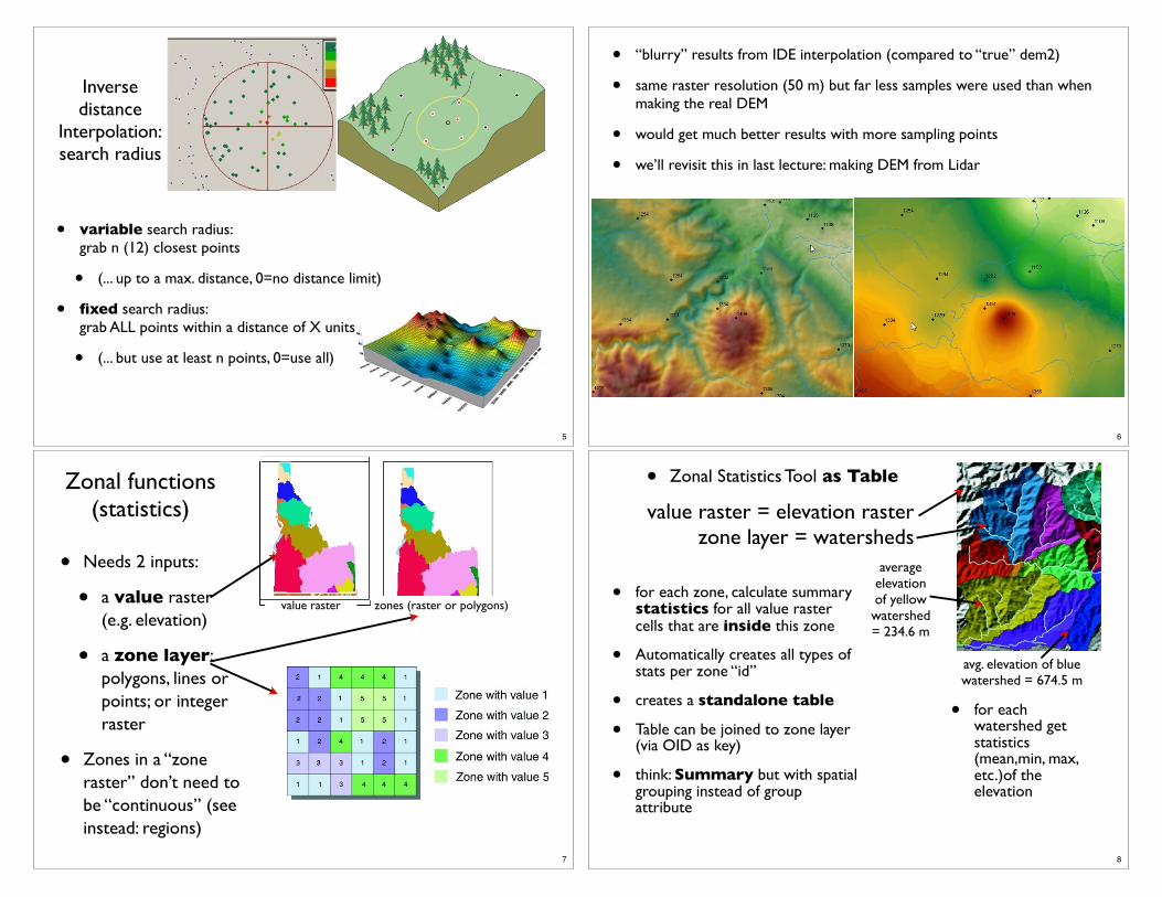
Interpolation• Need: point samples

(here: elevation, think GPS points)

• Go over all cells of an empty raster, for each cell:

• Grab all the closest point samples (here: within a radius around the cell)

• Do some spatial math with these point samples

• IDW: faster, Spline: smoother

• result: cell’s elevation

4

Inverse distance

Interpolation: search radius

• variable search radius: grab n (12) closest points

• (... up to a max. distance, 0=no distance limit)

• fixed search radius:grab ALL points within a distance of X units

• (... but use at least n points, 0=use all)

5

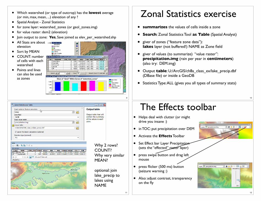
• “blurry” results from IDE interpolation (compared to “true” dem2)

• same raster resolution (50 m) but far less samples were used than when making the real DEM

• would get much better results with more sampling points

• we’ll revisit this in last lecture: making DEM from Lidar

6

Zonal functions (statistics)

• Needs 2 inputs:

• a value raster (e.g. elevation)

• a zone layer: polygons, lines or points; or integer raster

• Zones in a “zone raster” don’t need to be “continuous” (see instead: regions)

zones (raster or polygons)value raster

7

• for each zone, calculate summary statistics for all value raster cells that are inside this zone

• Automatically creates all types of stats per zone “id”

• creates a standalone table

• Table can be joined to zone layer (via OID as key)

• think: Summary but with spatial grouping instead of group attribute

• for each watershed get statistics (mean,min, max, etc.)of the elevation

value raster = elevation raster zone layer = watersheds

avg. elevation of blue watershed = 674.5 m

average elevation of yellow watershed = 234.6 m

• Zonal Statistics Tool as Table

8

• Which watershed (or type of outcrop) has the lowest average (or min, max, mean, ...) elevation of any ?

• Spatial Analyst - Zonal Statistics

• for zone layer: watershed_zones (or geol_zones.img)

• for value raster: dem2 (elevation)

• Join output to zone: Yes, Save joined as elev_per_watershed.shp

• All Stats are about elevation

• Sort by MEAN

• COUNT: numberof cells with eachwatershed

• Points and linescan also be usedas zones

9

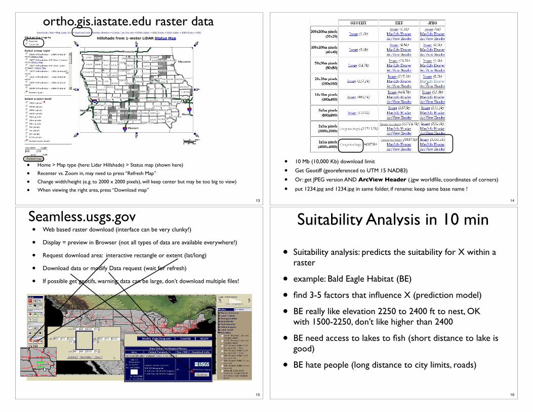
Zonal Statistics exercise• summarizes the values of cells inside a zone

• Search: Zonal Statistics Tool as Table (Spatial Analyst)

• giver of zones (“feature zone data”): lakes layer (not buffered!) NAME as Zone field

• giver of values (to summarize) “value raster”: precipitation.img (rain per year in centimeters)(also try: DEM.img)

• Output table: U:/ArcGIS/ch8a_class_ex/lake_precip.dbf (DBase file) or inside a GeoDB

• Statistics Type: ALL (gives you all types of summary stats)

10

Why 2 rows?COUNT?Why very similar MEAN?

optional: join lake_precip to lakes using NAME

11

The Effects toolbar• Helps deal with clutter (or might

drive you insane :)

• in TOC: put precipitation over DEM

• Activate the Effects Toolbar

• Set Effect bar Layer Precipitation (sets the “effected” raster layer)

• press swipe button and drag left mouse

• press flicker (500 ms) button (seizure warning :)

• Also: adjust contrast, transparency on the fly

12

ortho.gis.iastate.edu raster data

• Home > Map type (here: Lidar Hillshade) > Status map (shown here)

• Recenter vs. Zoom in, may need to press “Refresh Map”

• Change width/height (e.g. to 2000 x 2000 pixels), will keep center but may be too big to view)

• When viewing the right area, press “Download map”

13

• 10 Mb (10,000 Kb) download limit

• Get Geotiff (georeferenced to UTM 15 NAD83)

• Or: get JPEG version AND ArcView Header (.jgw worldfile, coordinates of corners)

• put 1234.jpg and 1234.jpg in same folder, if rename: keep same base name !

14

Seamless.usgs.gov• Web based raster download (interface can be very clunky!)

• Display = preview in Browser (not all types of data are available everywhere!)

• Request download area: interactive rectangle or extent (lat/long)

• Download data or modify Data request (wait for refresh)

• If possible get geotifs, warning: data can be large, don’t download multiple files!

15

Suitability Analysis in 10 min

• Suitability analysis: predicts the suitability for X within a raster

• example: Bald Eagle Habitat (BE)

• find 3-5 factors that influence X (prediction model)

• BE really like elevation 2250 to 2400 ft to nest, OK with 1500-2250, don’t like higher than 2400

• BE need access to lakes to fish (short distance to lake is good)

• BE hate people (long distance to city limits, roads)

16

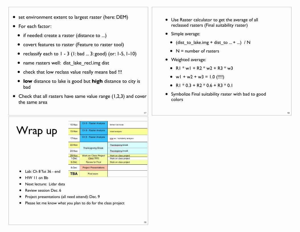
• set environment extent to largest raster (here: DEM)

• For each factor:

• if needed: create a raster (distance to ...)

• covert features to raster (Feature to raster tool)

• reclassify each to 1 - 3 (1: bad ... 3: good) (or: 1-5, 1-10)

• name rasters well: dist_lake_recl.img dist

• check that low reclass value really means bad !!!

• low distance to lake is good but high distance to city is bad

• Check that all rasters have same value range (1,2,3) and cover the same area

17

• Use Raster calculator to get the average of all reclassed rasters (Final suitability raster)

• Simple average:

• (dist_to_lake.img + dist_to ... + ...) / N

• N = number of rasters

• Weighted average:

• R1 * w1 + R2 * w2 + R3 * w3

• w1 + w2 + w3 = 1.0 (!!!!)

• R1 * 0.3 + R2 * 0.6 + R3 * 0.1

• Symbolize Final suitability raster with bad to good colors

18

Wrap up

• Lab: Ch 8 Tut 36 - end

• HW 11 on Bb

• Next lecture: Lidar data

• Review session Dec. 6

• Project presentations (all need attend): Dec. 9

• Please let me know what you plan to do for the class project

19