approximation schemes – a tutorial 1gwoegi/papers/ptas.pdf · approximation schemes – a...

Approximation Schemes – A Tutorial 1

Petra Schuurman 2 Gerhard J. Woeginger 3

1This is the preliminary version of a chapter of the book “Lectures on Scheduling”

edited by R.H. Mohring, C.N. Potts, A.S. Schulz, G.J. Woeginger, L.A. Wolsey, to

appear around 2011 [email protected]. Department of Mathematics and Computing Science,

Eindhoven University of Technology, P.O. Box 513, NL-5600 MB Eindhoven, The

[email protected]. Department of Mathematics and Computing Science, Eind-

hoven University of Technology, P.O. Box 513, NL-5600 MB Eindhoven, The Nether-

lands.

2

Summary: This tutorial provides an introduction into the area of polyno-mial time approximation schemes. The underlying ideas, the main tools, andthe standard approaches for the construction of such schemes are explained ingreat detail and illustrated in many examples and exercises. The tutorial alsodiscusses techniques for disproving the existence of approximation schemes.

Keywords: approximation algorithm, approximation scheme, PTAS, FPTAS,worst case analysis, performance guarantee, in-approximability, gap technique,L-reduction, APX, intractability, polynomial time, scheduling.

0.1 Introduction

All interesting problems are difficult to solve. This observation in particularholds true in algorithm oriented areas like combinatorial optimization, math-ematical programming, operations research, and theoretical computer sciencewhere researchers often face computationally intractable problems. Since solv-ing an intractable problem to optimality is a tough goal, these researchers usu-ally resort to simpler suboptimal approaches that yield decent solutions, whilehoping that those decent solutions come at least close to the true optimum. Anapproximation scheme is a suboptimal approach that provably works fast andthat provably yields solutions of very high quality. And that’s the topic of thischapter: Approximation schemes. Let us illustrate this concept by an exampletaken from the real world of Dilbert [1] cartoons.

Example 0.1.1 Let us suppose that you are the pointy-haired boss of the plan-ning department of a huge company. The top-managers of your company havedecided that the company is going to generate gigantic profit by constructing aspaceship that travels faster than light. Your department has to set up the sched-ule for this project. And of course, the top-managers want you to find a schedulethat minimizes the cost incurred by the company. So you ask your experiencedprogrammers Wally and Dilbert to determine such a schedule. Wally and Dil-bert tell you: “We can do that. Real programmers can do everything. And wepredict that the cost of the best schedule will be exactly one gazillion dollars.”You say: “Sounds great! Wonderful! Go ahead and determine this schedule! Iwill present it to our top-managers in the meeting tomorrow afternoon.” Butthen Wally and Dilbert say: “We cannot do that by tomorrow afternoon. Realprogrammers can do everything, but finding the schedule is going to take ustwenty-three and a half years.”

You are shocked by the incompetence of your employees, and you decide togive the task to somebody who is really smart. So you consult Dogbert, the dog ofDilbert. Dogbert tells you: “Call me up tomorrow, and I will have your schedule.The schedule is going to cost exactly two gazillion dollars.” You complain:“But Wally and Dilbert promised me that there is a schedule that only costs onegazillion dollars. I do not want to spend an extra gazillion dollars on it!” AndDogbert says: “Then please call me up again twenty-three and a half years from

0.1. INTRODUCTION 3

now. Or, you may call me up again the day after tomorrow, and I will have aschedule for you that only costs one and a half gazillion dollars. Or, you maycall me up again the day after the day after tomorrow, and I will have a schedulethat only costs one and a third gazillion dollars.” Now you become really curious:“What if I call you up exactly x days from now?” Dogbert: “Then I would havefound a schedule that costs at most 1 + 1/x gazillion dollars.”

Dogbert obviously has found an approximation scheme for the company’s toughscheduling problem: Within reasonable time (which means: x days) he can comefairly close (which means: at most a factor of 1+1/x away) to the true optimum(which means: one gazillion dollars). Note that as x becomes very large, thecost of Dogbert’s schedule comes arbitrarily close to the optimal cost. The goalof this chapter is to give you a better understanding of Dogbert’s technique. Wewill introduce you to the main ideas, and we will explain the standard tools forfinding approximation schemes. We identify three constructive approaches forgetting an approximation scheme, and we illustrate their underlying ideas bystating many examples and exercises. Of course, not every optimization problemhas an approximation scheme – this just would be too good to be true. We willexplain how one can recognize optimization problems with bad approximabilitybehavior. Currently there are only a few tools available for getting such in-approximability results, and we will discuss them in detail and illustrate themwith many examples.

The chapter uses the context of scheduling to present the techniques andtools around approximation schemes, and all the illustrating examples and ex-ercises are taken from the field of scheduling. However, the methodology isgeneral and it applies to all kinds of optimization problems in all kinds of areaslike networks, graph theory, geometry, etc.

——————————

In the following paragraphs we will give exact mathematical definitions ofthe main concepts in the area of approximability. For these paragraphs andalso for the rest of the chapter, we will assume that the reader is familiar withthe basic concepts in computational complexity theory that are listed in theAppendix Section 0.8.

An optimization problem is specified by a set I of inputs (or instances), bya set Sol(I) of feasible solutions for every input I ∈ I, and by an objectivefunction c that specifies for every feasible solution σ in Sol(I) an objectivevalue or cost c(σ). We will only consider optimization problems in which allfeasible solutions have non-negative cost. An optimization problem may eitherbe a minimization problem where the optimal solution is a feasible solution withminimum possible cost, or a maximization problem where the optimal solutionis a feasible solution with maximum possible cost. In any case, we will denotethe optimal objective value for instance I by Opt(I). By |I| we denote thesize of an instance I, i.e., the number of bits used in writing down I in some

4

fixed encoding. Now assume that we are dealing with an NP-hard optimizationproblem where it is difficult to find the exact optimal solution within polynomialtime in |I|. At the expense of reducing the quality of the solution, we can oftenget considerable speed-up in the time complexity. This motivates the followingdefinition.

Definition 0.1.2 (Approximation algorithms)Let X be a minimization (respectively, maximization) problem. Let ε > 0, andset ρ = 1+ε (respectively, ρ = 1−ε). An algorithm A is called a ρ-approximationalgorithm for problem X, if for all instances I of X it delivers a feasible solutionwith objective value A(I) such that

|A(I) − Opt(I)| ≤ ε · Opt(I). (0.1)

In this case, the value ρ is called the performance guarantee or the worst caseratio of the approximation algorithm A.

Note that for minimization problems the inequality in (0.1) becomes A(I) ≤ (1+ε)Opt(I), whereas for maximization problems it becomes A(I) ≥ (1−ε)Opt(I).Note furthermore that for minimization problems the worst case ratio ρ = 1+ εis a real number greater or equal to 1, whereas for maximization problemsthe worst case ratio ρ = 1 − ε is a real number from the interval [0, 1]. Thevalue ρ can be viewed as the quality measure of the approximation algorithm.The closer ρ is to 1, the better the algorithm is. A worst case ratio ρ = 0for a maximization problem, or a worst case ratio ρ = 106 for a minimizationproblem are of rather poor quality. The complexity class APX consists of allminimization problems that have a polynomial time approximation algorithmwith some finite worst case ratio, and of all maximization problems that have apolynomial time approximation algorithm with some positive worst case ratio.

Definition 0.1.3 (Approximation schemes)Let X be a minimization (respectively, maximization) problem.

• An approximation scheme for problem X is a family of (1 + ε)-approxi-mation algorithms Aε (respectively, (1− ε)-approximation algorithms Aε)for problem X over all 0 < ε < 1.

• A polynomial time approximation scheme (PTAS) for problem X is anapproximation scheme whose time complexity is polynomial in the inputsize.

• A fully polynomial time approximation scheme (FPTAS) for problem Xis an approximation scheme whose time complexity is polynomial in theinput size and also polynomial in 1/ε.

Hence, for a PTAS it would be acceptable to have a time complexity proportionalto |I|2/ε; although this time complexity is exponential in 1/ε, it is polynomialin the size of the input I exactly as we required in the definition of a PTAS.An FPTAS cannot have a time complexity that grows exponentially in 1/ε,

0.1. INTRODUCTION 5

but a time complexity proportional to |I|8/ε3 would be fine. With respect toworst case approximation, an FPTAS is the strongest possible result that we canderive for an NP-hard problem. Figure 0.1 illustrates the relationships betweenthe classes NP, APX, P, the class of problems that are pseudo-polynomiallysolvable, and the classes of problems that have a PTAS and FPTAS.

'

&

$

%

APX'

&

$

%

PTAS'

&

$

%

FPTAS

'

&

$

%

Pseudo-PolynomialTime

NP

P

Figure 0.1: Containment relations between some of the complexity classes dis-cussed in this chapter.

A little bit of history. The first paper with a polynomial time approximationalgorithm for an NP-hard problem is probably the paper [26] by Graham from1966. It studies simple heuristics for scheduling on identical parallel machines.In 1969, Graham [27] extended his approach to a PTAS. However, at that timethese were isolated results. The concept of an approximation algorithm wasformalized in the beginning of the 1970s by Garey, Graham & Ullman [21].The paper [45] by Johnson may be regarded as the real starting point of thefield; it raises the ‘right’ questions on the approximability of a wide range ofoptimization problems. In the mid-1970s, a number of PTAS’s was developedin the work of Horowitz & Sahni [42, 43], Sahni [69, 70], and Ibarra & Kim [44].

6

The terms ‘approximation scheme’, ‘PTAS’, ‘FPTAS’ are due to a seminal paperby Garey & Johnson [23] from 1978. Also the first in-approximability resultswere derived around this time; in-approximability results are results that showthat unless P=NP some optimization problem does not have a PTAS or thatsome optimization problem does not have a polynomial time ρ-approximationalgorithm for some specific value of ρ. Sahni & Gonzalez [71] proved thatthe traveling salesman problem without the triangle-inequality cannot have apolynomial time approximation algorithm with finite worst case ratio. Garey& Johnson [22] derived in-approximability results for the chromatic number ofa graph. Lenstra & Rinnooy Kan [58] derived in-approximability results forscheduling of precedence constrained jobs.

In the 1980s theoretical computer scientists started a systematic theoreticalstudy of these concepts; see for instance the papers Ausiello, D’Atri & Protasi[11], Ausiello, Marchetti-Spaccamela & Protasi [12], Paz & Moran [65], andAusiello, Crescenzi & Protasi [10]. They derived deep and beautiful character-izations of polynomial time approximable problems. These theoretical charac-terizations are usually based on the existence of certain polynomial time com-putable functions that are related to the optimization problem in a certain way,and the characterizations do not provide any help in identifying these functionsand in constructing the PTAS. The reason for this is of course that all thesecharacterizations implicitly suffer from the difficulty of the P=NP question.

Major breakthroughs that give PTAS’s for specific optimization problemswere the papers by Fernandez de la Vega & Lueker [20] on bin packing, byHochbaum & Shmoys [37, 38] on the scheduling problem of minimizing themakespan on an arbitrary number of parallel machines, by Baker [14] on manyoptimization problems on planar graphs (like maximum independent set, mini-mum vertex cover, minimum dominating set), and by Arora [5] on the Euclideantraveling salesman problem. In the beginning of the 1990s, Papadimitriou &Yannakakis [64] provided tools and ideas from computational complexity the-ory for getting in-approximability results. The complexity class APX was born;this class contains all optimization problems that possess a polynomial timeapproximation algorithm with a finite, positive worst case ratio. In 1992 Arora,Lund, Motwani, Sudan & Szegedy [6] showed that the hardest problems in APXcannot have a PTAS unless P=NP. For an account of the developments thatled to these in-approximability results see the NP-completeness column [46] byJohnson.

Organization of this chapter. Throughout the chapter we will distinguishbetween so-called positive results which establish the existence of some approx-imation scheme, and so-called negative results which disprove the existence ofgood approximation results for some optimization problem under the assump-tion that P 6=NP. Sections 0.2–0.5 are on positive results. First, in Section 0.2we introduce three general approaches for the construction of approximationschemes. These three approaches are then analyzed in detail and illustratedwith many examples in the subsequent three Sections 0.3, 0.4, and 0.5. In Sec-

0.2. HOW TO GET POSITIVE RESULTS 7

tion 0.6 we move on to methods for deriving negative results. At the end of eachof the Sections 0.3–0.6 there are lists of exercises. Section 0.7 contains a briefconclusion. Finally, the Appendix Section 0.8 gives a very terse introductioninto computational complexity theory.

Some remarks on the notation. Throughout the chapter, we use the stan-dard three-field α |β | γ scheduling notation (see for instance Graham, Lawler,Lenstra & Rinnooy Kan [28] and Lawler, Lenstra, Rinnooy Kan & Shmoys[55]). The field α specifies the machine environment, the field β specifies thejob environment, and the field γ specifies the objective function.

We denote the base two logarithm of a real number x by log(x), its naturallogarithm by ln(x), and its base b logarithm by logb(x). For a real number x,we denote by ⌊x⌋ the largest integer less or equal to x, and we denote by ⌈x⌉the smallest integer greater or equal to x. Note that ⌈x⌉ + ⌈y⌉ ≥ ⌊x + y⌋ and⌊x⌋ + ⌊y⌋ ≤ ⌈x + y⌉ hold for all real numbers x and y. A d-dimensional vector~v with coordinates vk (1 ≤ k ≤ d) will always be written in square bracketsas ~v = [v1, v2, . . . , vd]. For two d-dimensional vectors ~v = [v1, v2, . . . , vd] and~u = [u1, u2, . . . , ud] we write ~u ≤ ~v if and only if uk ≤ vk holds for 1 ≤ k ≤ d.For a finite set S, we denote its cardinality by |S|. For an instance I of acomputational problem, we denote its size by |I|, i.e., the number of bits thatare used for writing down I in some fixed encoding.

0.2 How to get positive results

Positive results in the area of approximation concern the design and analysis ofpolynomial time approximation algorithms and polynomial time approximationschemes. This section (and also the following three sections of this chapter)concentrate on such positive results; in this section we will only outline themain strategy. Assume that we need to find an approximation scheme for somefixed NP-hard optimization problem X . How shall we proceed?

Let us start by considering an exact algorithm A that solves problem Xto optimality. Algorithm A takes an instance I of X , processes it for sometime, and finally outputs the solution A(I) for instance I. See Figure 0.2 for anillustration. All known approaches to approximation schemes are based on thediagram depicted in this figure. Since the optimization problem X is difficultto solve, the exact algorithm A will have a bad (exponential) time complexityand will be far away from yielding a PTAS or yielding an FPTAS. How canwe improve the behavior of such an algorithm and bring it closer to a PTAS?The answer is to add structure to the diagram in Figure 0.2. This additionalstructure depends on the desired precision ε of approximation. If ε is large, thereshould be lots of additional structure. And as ε tends to 0, also the amountof additional structure should tend to 0 and should eventually disappear. Theadditional structure simplifies the situation and leads to simpler, perturbed andblurred versions of the diagram in Figure 0.2.

8

@@

��

@@

��

Instance I Algorithm A Output A(I)

Figure 0.2: Algorithm A solves instance I and outputs the feasible solutionA(I).

Note that the diagram consists of three well-separated parts: The inputto the left, the output to the right, and the execution of the algorithm A inthe middle. And these three well-separated parts give us three ways to addstructure to the diagram. The three ways will be discussed in the followingthree sections: Section 0.3 deals with the addition of structure to the input ofan algorithm, Section 0.4 deals with the addition of structure to the output of analgorithm, and Section 0.5 deals with the addition of structure to the executionof an algorithm.

0.3 Structuring the input

As first standard approach to the construction of approximation schemes wewill discuss the technique of adding structure to the input data. Here the mainidea is to turn a difficult instance into a more primitive instance that is easierto tackle. Then we use the optimal solution for the primitive instance to get agrip on the original instance. More formally, the approach can be described bythe following three-step procedure; see Figure 0.3 for an illustration.

(A) Simplify. Simplify instance I into a more primitive instanceI#. This simplification depends on the desired precision ε of ap-proximation; the closer ε is to zero, the closer instance I# shouldresemble instance I. The time needed for the simplification must bepolynomial in the input size.

(B) Solve. Determine an optimal solution Opt# for the simplifiedinstance I# in polynomial time.

(C) Translate back. Translate the solution Opt# for I# backinto an approximate solution App for instance I. This translationexploits the similarity between instances I and I#. In the ideal case,App will stay close to Opt# which in turn is close to Opt. In thiscase we find an excellent approximation.

0.3. STRUCTURING THE INPUT 9

AA##AA��LLHH ((E

E AACC��

EE "" D

DD��XX��

I I#

66

Opt

-

-Simplification

�

�Translate backApp

66Solve

Opt#

Figure 0.3: Structuring the input. Instance I is very complicated and irregularlyshaped, and it would be difficult to go directly from I to its optimal solutionOpt. Hence, one takes the detour via the simplified instance I# for which itis easy to obtain an optimal solution Opt#. Then one translates Opt# intoan approximate solution App for the original instance I. Let us hope that theobjective value of App is close to that of Opt!

Of course, finding the right simplification in step (A) is an art. If instanceI# is chosen too close to the original instance I, then I# might still be NP-hard to solve to optimality. On the other hand, if instance I# is chosen toofar away from the original instance I, then solving I# will not tell us anythingabout how to solve I. Under-simplifications (for instance, setting I# = I) andover-simplifications (for instance, setting I# = ∅) are equally dangerous. Thefollowing approaches to simplifying the input often work well.

Rounding. The simplest way of adding structure to the input isto round some of the numbers in the input. For instance, we mayround all job lengths to perfect powers of two, or we may roundnon-integral due dates up to the closest integers.

Merging. Another way of adding structure is to merge small piecesinto larger pieces of primitive shape. For instance, we may mergea huge number of tiny jobs into a single job with processing timeequal to the processing time of the tiny jobs, or into a single jobwith processing time equal to the processing time of the tiny jobsrounded to some nice value.

10

Cutting. Yet another way of adding structure is to cut awayirregular shaped pieces from the instance. For instance, we mayremove a small set of jobs with a broad spectrum of processing timesfrom the instance.

Aligning. Another way of adding structure to the input is to alignthe shapes of several similar items. For instance, we may replacethirty-six different jobs of roughly equal length by thirty-six identicalcopies of the job with median length.

The approach of structuring the input has a long history that goes back(at least) to the early 1970s. In 1974 Horowitz & Sahni [42] used it to attackpartition problems. In 1975 Sahni [69] applied it to the 0-1 knapsack problem,and in 1976 Sahni [70] applied it to makespan minimization on two parallelmachines. Other prominent approximation schemes that use this approach canbe found in the paper of Fernandez de la Vega & Lueker [20] on bin packing,and in the paper by Hochbaum & Shmoys [37] on makespan minimization onparallel machines (the Hochbaum & Shmoys result will be discussed in detailin Section 0.3.2). Arora [5] applied simplification of the input as a kind ofpreprocessing step in his PTAS for the Euclidean traveling salesman problem,and Van Hoesel & Wagelmans [77] used it to develop an FPTAS for the economiclot-sizing problem.

In the following three sections, we will illustrate the technique of simplify-ing the input data with the help of three examples. Section 0.3.1 deals withmakespan minimization on two identical machines, Section 0.3.2 deals withmakespan minimization on an arbitrary number of identical machines, and Sec-tion 0.3.3 discusses total tardiness on a single machine. Section 0.3.4 containsa number of exercises.

0.3.1 Makespan on two identical machines

The problem. In the scheduling problem P2 | |Cmax the input consists of njobs Jj (j = 1, . . . , n) with positive integer processing times pj . All jobs areavailable at time zero, and preemption is not allowed. The goal is to schedulethe jobs on two identical parallel machines so as to minimize the maximum jobcompletion time, the so-called makespan Cmax. In other words, we would like toassign roughly equal amounts of processing time to both machines (but withoutcutting any of the jobs); the objective value is the total processing time on themachine that finishes last. Throughout this section (and also in all subsequentsections), the objective value of an optimal schedule will be denoted by Opt.

The problem P2 | |Cmax is NP-hard in the ordinary sense (Karp [48]).We denote by psum =

∑nj=1 pj the overall job processing time and by

pmax = maxnj=1 pj the length of the longest job. It is easy to see that for

L = max{ 12psum, pmax}

L ≤ Opt. (0.2)

Indeed, pmax is a lower bound on Opt (the longest job must be entirely processedon one of the two machines) and also 1

2psum is a lower bound on Opt (the overall


job processing time psum must be assigned to the two machines, and even if wereach a perfect split the makespan is still at least 1

2psum).In this section, we will construct a PTAS for problem P2 | |Cmax by applying

the technique of simplifying the input. Later in this chapter we will meet thisproblem again, once in Section 0.4.1 and once in Section 0.5.1: Since P2 | |Cmax

is very simple to state and since it is a very basic problem in scheduling, it isthe perfect candidate to illustrate all the three main approaches to approxima-tion schemes. As we will see, the three resulting approximation schemes arecompletely independent and very different from each other.

(A) How to simplify an instance. We translate an arbitrary instance Iof P2 | |Cmax into a corresponding simplified instance I#. The jobs in I areclassified into big jobs and small jobs ; the classification depends on a precisionparameter 0 < ε < 1.

• A job Jj is called big if it has processing time pj > εL. The instance I#

contains all the big jobs from instance I.

• A job Jj is called small if it has processing time pj ≤ εL. Let S denotethe total processing time of all small jobs in I. Then instance I# contains⌊S/(εL)⌋ jobs of length εL. In a pictorial setting, the small jobs in I arefirst glued together to give a long job of length S, and then this long jobis cut into lots of chunks of length εL (if the last chunk is strictly smallerthan εL, then we simply disregard it).

And this completes the description of the simplified instance I#. Why do weclaim that I# is a simplified version of instance I? Well, the big jobs in I arecopied directly into I#. For the small jobs in I, we imagine that they are likesand; their exact size does not matter, but we must be able to fit all this sandinto the schedule. Since the chunks of length εL in I# cover about the samespace as the small jobs in I do, the most important properties of the small jobsare also present in instance I#.

We want to argue that the optimal makespan Opt# of I# is fairly close tothe optimal makespan Opt of I: Denote by Si (1 ≤ i ≤ 2) the total size of allsmall jobs on machine Mi in an optimal schedule for I. On Mi, leave every bigjob where it is, and replace the small jobs by ⌈Si/(εL)⌉ chunks of length εL.Since

⌈S1/(εL)⌉ + ⌈S2/(εL)⌉ ≥ ⌊S1/(εL) + S2/(εL)⌋ = ⌊S/(εL)⌋,this process assigns all the chunks of length εL to some machine. By assign-ing the chunks, we increase the load of Mi by at most ⌈Si/(εL)⌉εL − Si ≤(Si/(εL) + 1) εL − Si = εL. The resulting schedule is a feasible schedule forinstance I#. We conclude that

Opt# ≤ Opt + εL ≤ (1 + ε)Opt. (0.3)

Note that the stronger inequality Opt# ≤ Opt will not in general hold. Con-sider for example an instance that consists of six jobs of length 1 with ε = 2/3.

12

Then Opt = L = 3, and all the jobs are small. In I# they are replaced by 3chunks of length 2, and this leads to Opt# = 4 > Opt.

(B) How to solve the simplified instance. How many jobs are there ininstance I#? When we replaced the small jobs in instance I by the chunks ininstance I#, we did not increase the total processing time. Hence, the totalprocessing time of all jobs in I# is at most psum ≤ 2L. Since each job in I# haslength at least εL, there are at most 2L/(εL) = 2/ε jobs in instance I#. Thenumber of jobs in I# is bounded by a finite constant that only depends on εand thus is completely independent of the number n of jobs in I.

Solving instance I# is easy as pie! We may simply try all possible schedules!Since each of the 2/ε jobs is assigned to one of the two machines, there are atmost 22/ε possible schedules, and the makespan of each of these schedules canbe determined in O(2/ε) time. So, instance I# can be solved in constant time!Of course this ‘constant’ is huge and grows exponentially in 1/ε, but after allour goal is to get a PTAS (and not an FPTAS), and so we do not care at allabout the dependence of the time complexity on 1/ε.

(C) How to translate the solution back. Consider an optimal schedule σ#

for the simplified instance I#. For i = 1, 2 we denote by L#i the load of machine

Mi in this optimal schedule, by B#i the total size of the big jobs on Mi, and by

S#i the total size of the chunks of small jobs on Mi. Clearly, L#

i = B#i + S#

i

and

S#1 + S#

2 = εL · ⌊ S

εL⌋ > S − εL. (0.4)

We construct the following schedule σ for I: Every big job is put onto the samemachine as in schedule σ#. How shall we handle the small jobs? We reserve aninterval of length S#

1 + 2εL on machine M1, and an interval of length S#2 on

machine M2. We then greedily put the small jobs into these reserved intervals:First, we start packing small jobs into the reserved interval on M1, until wemeet some small job that does not fit in any more. Since the size of a small jobis at most εL, the total size of the packed small jobs on M1 is at least S#

1 + εL.

Then the total size of the unpacked jobs is at most S − S#1 − εL, and by (0.4)

this is bounded from above by S#2 . Hence, all remaining unpacked small jobs

together will fit into the reserved interval on machine M2. This completes thedescription of schedule σ for instance I.

Let us compare the loads L1 and L2 of the machines in σ to the machinecompletion times L#

1 and L#2 in schedule σ#. Since the total size of the small

jobs on Mi is at most S#i + 2εL, we conclude that

Li ≤ B#i +(S#

i +2εL) = L#i +2εL ≤ (1+ε)Opt+2εOpt = (1+3ε)Opt.

(0.5)

In this chain of inequalities we have used L ≤ Opt from (0.2), and L#i ≤

Opt# ≤ (1+ ε)Opt which follows from (0.3). Hence, the makespan of schedule


σ is at most a factor 1+3ε above the optimum makespan. Since 3ε can be madearbitrary close to 0, we finally have reached the desired PTAS for P2 | |Cmax.

Discussion. At this moment, the reader might wonder whether for designingthe PTAS, it is essential whether we round the numbers up or whether wedo round them down. If we are dealing with the makespan criterion, then itusually is not essential. If the rounding is done in a slightly different way, allour claims and all the used inequalities still hold in some slightly modified form.For example, suppose that we had defined the number of chunks in instance I#

to be ⌈S/(εL)⌉ instead of ⌊S/(εL)⌋. Then inequality (0.3) could be replaced byOpt# ≤ (1 + 2ε)Opt. All our calculations could by updated in an appropriateway, and eventually they would yield a worst case guarantee of 1 + 4ε. Thisagain yields a PTAS. Hence, there is lots of leeway in our argument and thereis sufficient leeway to do the rounding in a different way.

The time complexity of our PTAS is linear in n, but exponential in 1/ε: Theinstance I# is easily determined in O(n) time, the time for solving I# growsexponentially with 1/ε, and translating the solution back can again be donein O(n) time. Is this the best time complexity we can expect from a PTASfor P2 | |Cmax? No, there is even an FPTAS (but we will have to wait tillSection 0.5.1 to see it).

How would we tackle makespan minimization on m ≥ 3 machines? First,we should redefine L = max{ 1

mpsum, pmax} instead of L = max{ 12psum, pmax} so

that the crucial inequality (0.2) is again satisfied. The simplification step (A)and the translation step (C) do not need major modifications. Exercise 0.3.1in Section 0.3.4 asks the reader to fill in the necessary details. However, thesimplified instance I# in step (B) now may consist of roughly m/ε jobs, andso the time complexity becomes exponential in m/ε. As long as the number mof machines is a fixed constant, this approach works fine and gives us a PTASfor Pm | |Cmax. But if m is part of the input, the approach breaks down. Thecorresponding problem P | |Cmax is the subject of the following section.

0.3.2 Makespan on an arbitrary number of identical ma-

chines

The problem. In the scheduling problem P | |Cmax the input consists of n jobsJj (j = 1, . . . , n) with positive integer processing times pj and of m identicalmachines. The goal is to find a schedule that minimizes the makespan; theoptimal makespan will be denoted by Opt. This problem generalizes P2 | |Cmax

from Section 0.3.1. The crucial difference to P2 | |Cmax is that the numberm of machines is part of the input. Therefore, a polynomial time algorithmdealing with this problem must have a time complexity that is also polynomiallybounded in m.

The problem P | |Cmax is NP-hard in the strong sense (Garey & John-son [24]). Analogously to Section 0.3.1, we define psum =

∑nj=1 pj , pmax =

14

maxnj=1 pj , and L = max{ 1

mpsum, pmax}. We claim that

L ≤ Opt ≤ 2L. (0.6)

Indeed, since 1mpsum and pmax are lower bounds on Opt, L is also a lower bound

on Opt. We show that 2L is an upper bound on Opt by exhibiting a schedulewith makespan at most 2L. We assign the jobs one by one to the machines;every time a job is assigned, it is put on a machine with the current minimalworkload. As this minimal workload is at most 1

mpsum and as the newly assignedjob adds at most pmax to the workload, the makespan always remains boundedby 1

mpsum + pmax ≤ 2L.We will now construct a PTAS for problem P | |Cmax by the technique of

simplifying the input. Many ideas and arguments from Section 0.3.1 directlycarry over to P | |Cmax. We mainly concentrate on the additional ideas thatwere developed by Hochbaum & Shmoys [37] and by Alon, Azar, Woeginger &Yadid [3] to solve the simplified instance in step (B).

(A) How to simplify an instance. To simplify the presentation, we assumethat ε = 1/E for some integer E. Jobs are classified into big and small ones,exactly as in Section 0.3.1. The small jobs with total size S are replaced be⌊S/(εL)⌋ chunks of length εL, exactly as in Section 0.3.1. The big jobs, however,are handled in a different way: For each big job Jj in I, the instance I# contains

a corresponding job J#j with processing time p#

j = ε2L⌊pj/(ε2L)⌋, i.e., p#j is

obtained by rounding pj down to the next integer multiple of ε2L. Note that

pj ≤ p#j + ε2L ≤ (1 + ε)p#

j holds. This yields the simplified instance I#.

As in Section 0.3.1 it can be shown that the optimal makespan Opt# of I#

fulfills Opt# ≤ (1+ε)Opt. The main difference in the argument is that the bigjobs in I# may be slightly smaller than their counterparts in instance I. Butthis actually works in our favor, since replacing jobs by slightly smaller ones canonly decrease the makespan (or leave it unchanged), but can never increase it.With (0.6) and the definition ε = 1/E, we get

Opt# ≤ 2(1 + ε)L = (2E2 + 2E) ε2L. (0.7)

In I# the processing time of a rounded big job lies between εL and L. Hence,it is of the form kε2L where k is an integer with E ≤ k ≤ E2. Note thatεL = Eε2L, and thus also the length of the chunks can be written in the formkε2L. For k = E, . . . , E2, we denote by nk the number of jobs in I# whose

processing time equals kε2L. Notice that n ≥ ∑E2

k=E nk. A compact way ofrepresenting I# is by collecting all the data in the vector ~n = [nE , . . . , nE2 ].

(B) How to solve the simplified instance. This step is more demandingthan the trivial solution we used in Section 0.3.1. We will formulate the simpli-fied instance as an integer linear program whose number of integer variables isbounded by some constant in E (and thus is independent of the input size). Andthen we can apply machinery from the literature for integer linear programs offixed dimension to get a solution in polynomial time!


We need to introduce some notation to describe the possible schedules forinstance I#. The packing pattern of a machine is a vector ~u = [uE, . . . , uE2 ],where uk is the number of jobs of length kε2L assigned to that machine. For

every vector ~u we denote C(~u) =∑E2

k=E uk · k. Note that the workload of the

corresponding machine equals∑E2

k=E uk · kε2L = C(~u) ε2L. We denote by Uthe set of all packing patterns ~u for which C(~u) ≤ 2E2 + 2E, i.e., for which thecorresponding machine has a workload of at most (2E2 + 2E) ε2L. Because ofinequality (0.7), we only need to consider packing patterns in U if we want tosolve I# to optimality. Since each job has length at least Eε2L, each packingpattern ~u ∈ U consists of at most 2E+2 jobs. Therefore |U | ≤ (E2−E+1)2E+3

holds, and the cardinality of U is bounded by a constant in E (= 1/ε) that doesnot depend on the input. This property is important, as our integer linearprogram will have 2|U | + 1 integer variables.

Now consider some fixed schedule for instance I#. For each vector ~u ∈ U ,we denote by x~u the numbers of machines with packing pattern ~u. The 0-1-variable y~u serves as an indicator variable for x~u: It takes the value 0 if x~u = 0,and it takes the value 1 if x~u ≥ 1. Finally, we use the variable z to denotethe makespan of the schedule. The integer linear program (ILP) is depicted inFigure 0.4.

min z

s.t.∑

~u∈U x~u = m∑

~u∈U x~u · ~u = ~n

y~u ≤ x~u ≤ m · y~u ∀ ~u ∈ U

C(~u) · y~u ≤ z ∀ ~u ∈ U

x~u ≥ 0, x~u integer ∀ ~u ∈ U

y~u ∈ {0, 1} ∀ ~u ∈ U

z ≥ 0, z integer

Figure 0.4: The integer linear program (ILP) in Section 0.3.2.

The objective is to minimize the value z; the makespan of the underlyingschedule will be zε2L which is proportional to z. The first constraint states thatexactly m machines must be used. The second constraint (which in fact is aset of E2 − E + 1 constraints) ensures that all jobs can be packed; recall that~n = [nE , . . . , nE2 ]. The third set of constraints ties x~u to its indicator variabley~u: x~u = 0 implies y~u = 0, and x~u ≥ 1 implies y~u = 1 (note that each variable x~u

takes an integer value between 0 and m). The fourth set of constraints ensuresthat zε2L is at least as large as the makespan of the underlying schedule: If thepacking pattern ~u is not used in the schedule, then y~u = 0 and the constraint

16

boils down to z ≥ 0. If the packing pattern ~u is used in the schedule, then y~u = 1and the constraint becomes z ≥ C(~u) which is equivalent to zε2L ≥ C(~u) ε2L.The remaining constraints are just integrality and non-negativity constraints.Clearly, the optimal makespan Opt# of I# equals z∗ε2L where z∗ is the optimalobjective value z∗ of (ILP).

The number of integer variables in (ILP) is 2|U | + 1, and we have alreadyobserved that this is a constant that does not depend at all on the instanceI. We now apply Lenstra’s famous algorithm [57] to solve (ILP). The timecomplexity of Lenstra’s algorithm is exponential in the the number of variables,but polynomial in the logarithms of the coefficients. The coefficients in (ILP) areat most max{m, n, 2E2+2E}, and so (ILP) can be solved within an overall time

complexity of O(logO(1)(m + n)). Note that here the hidden constant dependsexponentially on 1/ε. To summarize, we can solve the simplified instance I# inpolynomial time.

(C) How to translate the solution back. We proceed as in step (C) inSection 0.3.1: If in an optimal schedule for I# the total size of chunks on machineMi equals S#

i , then we reserve a time interval of length S#i + 2εL on Mi and

greedily pack the small jobs into all these reserved intervals. There is sufficientspace to pack all small jobs. Big jobs in I# are replaced by their counterpartsin I. Since pj ≤ (1 + ε)p#

j holds, this may increase the total processing time ofbig jobs on Mi by at most a factor of 1 + ε. Similarly as in (0.5) we concludethat

Li ≤ (1 + ε)B#i + S#

i + 2εL ≤ (1 + ε)Opt#i + 2εL

≤ (1 + ε)2Opt + 2εOpt = (1 + 4ε + ε2)Opt.

Here we used Opt# ≤ (1 + ε)Opt, and we used (0.6) to bound L from above.Since the term 4ε+ ε2 can be made arbitrarily close to 0, this yields the PTAS.

Discussion. The polynomial time complexity of the above PTAS heavily re-lies on solving (ILP) by Lenstra’s method, which really is heavy machinery.Are there other, simpler possibilities for solving the simplified instance I# inpolynomial time? Yes, there are. Hochbaum & Shmoys [37] use a dynamicprogramming approach with time complexity polynomial in n. However, thedegree of this polynomial time complexity is proportional to |U |. This dynamicprogram is outlined in Exercise 0.3.3 in Section 0.3.4.

0.3.3 Total tardiness on a single machine

The problem. In the scheduling problem 1 | | ∑Tj , the input consists of n

jobs Jj (j = 1, . . . , n) with positive integer processing times pj and integer duedates dj . All jobs are available for processing at time zero, and preemptionis not allowed. We denote by Cj the completion time of job Jj in some fixedschedule. Then the tardiness of job Jj in this schedule is Tj = max{0, Cj − dj},i.e., the amount of time by which Jj violates its deadline. The goal is to schedule


the jobs on a single machine such that the total tardiness∑n

j=1 Tj is minimized.Clearly, in an optimal schedule the jobs will be processed without any idle timebetween consecutive jobs and the optimal schedule can be fully specified by apermutation π∗ of the n jobs. We use Opt to denote the objective value of theoptimal schedule π∗.

The problem 1 | | ∑Tj is NP-hard in the ordinary sense (Du & Leung [18]).

Lawler [53] developed a dynamic programming formulation for 1 | | ∑Tj . The

(pseudo-polynomial) time complexity of this dynamic program is O(n5TEDD).Here TEDD denotes the maximum tardiness in the EDD-schedule, i.e., the sched-ule produced by the earliest-due-date rule (EDD-rule). The EDD-rule sequencesthe jobs in order of non-decreasing due date; this rule is easy to implementin polynomial time O(n log n), and it is well-known that the resulting EDD-schedule minimizes the maximum tardiness maxTj. Hence TEDD can be com-puted in polynomial time; this is important, as our simplification step will explic-itly use the value of TEDD. In case TEDD = 0 holds, all jobs in the EDD-schedulehave tardiness 0 and the EDD-schedule constitutes an optimal solution to prob-lem 1 | | ∑

Tj . Therefore, we will only deal with the case TEDD > 0. Moreover,since in the schedule that minimizes the total tardiness, the most tardy job hastardiness at least TEDD, we have

TEDD ≤ Opt. (0.8)

We will not discuss any details of Lawler’s dynamic program here, since we willonly use it as a black box. For our purposes, it is sufficient to know its timecomplexity O(n5TEDD) in terms of n and TEDD.

(A) How to simplify an instance. Following Lawler [54] we will nowadd structure to the input, and thus eventually get an FPTAS. The additionalstructure depends on the following parameter Z.

Z :=2ε

n(n + 3)· TEDD

Note that TEDD > 0 yields Z > 0. We translate an arbitrary instance I of1 | | ∑

Tj into a corresponding simplified instance I#. The processing time of

the j-th job in I# equals p#j = ⌊pj/Z⌋, and its due date equals d#

j = ⌈dj/Z⌉.The alert reader will have noticed that scaling the data by Z causes the

processing times and due dates in instance I# to be very far away from thecorresponding processing times and due dates in the original instance I. Howcan we claim that I# is a simplified version of I when it is so far away frominstance I? One way of looking at this situation is that in fact we producethe simplified instance I# in two steps. In the first step, the processing timesin I are rounded down to the next integer multiple of Z, and the due datesare rounded up to the next integer multiple of Z. This yields the intermediateinstance I ′ in which all the data are divisible by Z. In the second step we scaleall processing times and due dates in I ′ by Z, and thus arrive at the instanceI# with much smaller numbers. Up to the scaling by Z, the instances I ′ and

18

I# are equivalent. See Figure 0.5 for a listing of the variables in these threeinstances.

Instance I I ′ I#

length of Jj pj p′j = ⌊pj/Z⌋Z p#j = ⌊pj/Z⌋

p′j ≤ pj p#j = p′j/Z

due date of Jj dj d′j = ⌈dj/Z⌉Z d#j = ⌈dj/Z⌉

d′j ≥ dj d#j = d′j/Z

optimal value Opt Opt′ (≤ Opt) Opt# (= Opt′/Z)

Figure 0.5: The notation used in the PTAS for 1 | | ∑Tj in Section 0.3.3.

(B) How to solve the simplified instance. We solve instance I# by apply-ing Lawler’s dynamic programming algorithm, whose time complexity dependson the number of jobs and on the maximum tardiness in the EDD-schedule.Clearly, there are n jobs in instance I#. What about the maximum tardiness?Let us consider the EDD-sequence π for the original instance I. When we moveto I ′ and to I#, all the due dates are changed in a monotone way and there-fore π is also an EDD-sequence for the jobs in the instances I ′ and I#. Whenwe move from I to I ′, processing times cannot increase and due dates cannotdecrease. Therefore, T ′

EDD ≤ TEDD. Since I# results from I ′ by simple scaling,we conclude that

T #EDD = T ′

EDD/Z ≤ TEDD/Z = n(n + 3)/(2ε).

Consequently T #EDD is O(n2/ε). With this the time complexity of Lawler’s

dynamic program for I# becomes O(n7/ε), which is polynomial in n and in1/ε. And that is exactly the type of time complexity that we need for anFPTAS! So, the simplified instance is indeed easy to solve.

(C) How to translate the solution back. Consider an optimal job sequencefor instance I#. To simplify the presentation, we renumber the jobs in sucha way that this optimal sequence becomes J1, J2, J3, . . . , Jn. Translating thisoptimal solution back to the original instance I is easy: We take the samesequence for the jobs in I to get an approximate solution. We now want toargue that the objective value of this approximate solution is very close to theoptimal objective value. This is done by exploiting the structural similaritiesbetween the three instances I, I ′, and I#.

We denote by Cj and Tj the completion time and the tardiness of the j-th

job in the schedule for I, and by C#j and T #

j the completion time and the

tardiness of the j-th job in the schedule for instance I#. By the definition of


p#j and d#

j , we have pj ≤ Zp#j + Z and dj > Zd#

j − Z. This yields for thecompletion times Cj (j = 1, . . . , n) in the approximate solution that

Cj =

j∑

i=1

pj ≤ Z

j∑

i=1

p#j + jZ = Z · C#

j + jZ.

As a consequence,

Tj = max{0, Cj−dj} ≤ max{0, (Z·C#j +jZ)−(Zd#

j −z)} ≤ Z·T #j +(j+1)Z.

This finally leads to

n∑

j=1

Tj ≤n∑

j=1

Z · T #j +

1

2n(n + 3) · Z ≤ Opt + εTEDD ≤ (1 + ε)Opt.

Let us justify the correctness of the last two inequalities above. The penultimateinequality is justified by comparing instance I ′ to instance I. Since I ′ is a scaledversion of I#, we have

∑nj=1 Z · T #

j = Z · Opt# = Opt′. Since in I ′ the jobs

are shorter and have less restrictive due dates than in I, we have Opt′ ≤ Opt.The last inequality follows from the observation (0.8) in the beginning of thissection. To summarize, for each ε > 0 we can find within a time of O(n7/ε) anapproximate schedule whose objective value is at most (1+ ε)Opt. And that isexactly what is needed for an FPTAS!

0.3.4 Exercises

Exercise 0.3.1. Construct a PTAS for Pm | |Cmax by appropriately modifyingthe approach described in Section 0.3.1. Work with L = max{ 1

mpsum, pmax},and use the analogous definition of big and small jobs in the simplification step(A). Argue that the inequality (0.3) is again satisfied. Modify the translationstep (C) appropriately so that all small jobs are packed. What is your worstcase guarantee in terms of ε and m? How does your time complexity dependon ε and m?

Exercise 0.3.2. In the PTAS for P2 | |Cmax in Section 0.3.1, we replaced thesmall jobs in instance I by lots of chunks of length εL in instance I#. Considerthe following alternative way of handling the small jobs in I: Put all the smalljobs into a canvas bag. While there are at least two jobs with lengths smallerthan εL in the bag, merge two such jobs. That is, repeatedly replace two jobswith processing times p′, p′′ ≤ εL by a single new job of length p′ + p′′. Thesimplified instance I#

alt consists of the final contents of the bag.

Will this lead to another PTAS for P2 | |Cmax? Does the inequality (0.3)still hold true? How can you bound the number of jobs in the simplified instanceI#alt? How would you translate an optimal schedule for I#

alt into an approximateschedule for I?

20

Exercise 0.3.3. This exercise deals with the dynamic programming approachof Hochbaum & Shmoys [37] for the simplified instance I# of P | |Cmax. Thisdynamic progam has already been mentioned at the end of Section 0.3.2, andwe will use the notation of this section in this exercise.

Let V be the set of integer vectors that encode subsets of the jobs in I#,i.e. V = {~v : ~0 ≤ ~v ≤ ~n}. For every ~v ∈ V and for every i, 0 ≤ i ≤ m, denoteby F (i, ~v) the makespan of the optimal schedule for the jobs in ~v on exactly imachines that only uses packing patterns from U . If no such schedule exists weset F (i, ~v) = +∞. For example, F (1, ~v) = C(~v) ε2L if ~v ∈ U , and F (1, ~v) = +∞if ~v 6∈ U .

(a) Show that the cardinality of V is bounded by a polynomial in n. Howdoes the degree of this polynomial depend on ε and E?

(b) Find a recurrence relation that for i ≥ 2 and ~v ∈ V expresses the valueF (i, ~v) in terms of the values F (i − 1, ~v − ~u) with ~u ≤ ~v.

(c) Use this recurrence relation to compute the value F (m,~n) in polynomialtime. How does the time complexity depend on n?

(d) Argue that the optimal makespan for I# equals F (m,~n). How can you getthe corresponding optimal schedule? [Hint: Store some extra informationin the dynamic program.]

Exercise 0.3.4. Consider n jobs Jj (j = 1, . . . , n) with positive integer pro-cessing times pj on three identical machines. The goal is to find a schedule withmachine loads L1, L2, L3 that minimizes the value L2

1 + L22 + L2

3, the sum ofsquared machine loads.

Construct a PTAS for this problem by following the approach described inSection 0.3.1. Construct a PTAS for minimizing the sum of squared machineloads when the number m of machines is part of the input by following the ap-proach described in Section 0.3.2. For a more general discussion of this problem,see Alon, Azar, Woeginger & Yadid [3].

Exercise 0.3.5. Consider n jobs Jj (j = 1, . . . , n) with positive integer pro-cessing times pj on three identical machines M1, M2, and M3, together witha positive integer T . You have already agreed to lease all three machinesfor T time units. Hence, if machine Mi completes at time Li ≤ T , thenyour cost for this machine still is proportional to T . If machine Mi com-pletes at time Li > T , then you have to pay extra for the overtime, and yourcost is proportional to Li. To summarize, your goal is to minimize the valuemax{T, L1} + max{T, L2} + max{T, L3}, your overall cost.

Construct a PTAS for this problem by following the approach described inSection 0.3.1. Construct a PTAS for minimizing the corresponding objectivefunction when the number m of machines is part of the input by followingthe approach described in Section 0.3.2. For a more general discussion of thisproblem, see Alon, Azar, Woeginger & Yadid [3].


Exercise 0.3.6. Consider n jobs Jj (j = 1, . . . , n) with positive integer pro-cessing times pj on two identical machines. The goal is to find a schedule withmachine loads L1 and L2 that minimizes the following objective value:

(a) |L1 − L2|

(b) max{L1, L2}/ min{L1, L2}

(c) (L1 − L2)2

(d) L1 + L2 + L1 · L2

(e) max{L1, L2/2}

For which of these problems can you get a PTAS? Can you prove statementsanalogous to inequality (0.3) in Section 0.3.1? For the problems where you failto get a PTAS, discuss where and why the approach of Section 0.3.1 breaksdown.

Exercise 0.3.7. Consider two instances I and I ′ of 1 | | ∑Tj with n jobs,

processing times pj and p′j , and due dates dj and d′j . Denote by Opt and

Opt′ the respective optimal objective values. Furthermore, let ε > 0 be a realnumber. Prove or disprove:

(a) If pj ≤ (1 + ε)p′j and dj = d′j for 1 ≤ j ≤ n, then Opt ≤ (1 + ε)Opt′.

(b) If dj ≥ (1+ε)d′j and pj ≤ (1+ε)p′j for 1 ≤ j ≤ n, then Opt ≤ (1+ε)Opt′.

(c) If d′j ≤ (1 − ε)dj and pj = p′j for 1 ≤ j ≤ n, then Opt ≤ (1 − ε)Opt′.

Exercise 0.3.8. In the problem 1 | | ∑wjTj the input consists of n jobs Jj

(j = 1, . . . , n) with positive integer processing times pj, integer due dates dj ,and positive integer weights wj . The goal is to schedule the jobs on a singlemachine such that the total weighted tardiness

∑wjTj is minimized.

Can you modify the approach in Section 0.3.3 so that it yields a PTAS for1 | | ∑

wjTj? What are the main obstacles? Consult the paper by Lawler [53]to learn more about the computational complexity of 1 | | ∑

wjTj !

Exercise 0.3.9. Consider the problem 1 | rj |∑

Cj whose input consists of njobs Jj (j = 1, . . . , n) with processing times pj and release dates rj . In a feasibleschedule for this problem, no job Jj is started before its release date rj . Thegoal is to find a feasible schedule of the jobs on a single machine such that thetotal job completion time

∑Cj is minimized.

Consider two instances I and I ′ of 1 | rj |∑

Cj with n jobs, processing timespj and p′j , and release dates rj and r′j . Denote by Opt and Opt′ the respectiveoptimal objective values. Furthermore, let ε > 0 be a real number. Prove ordisprove:

(a) If pj ≤ (1 + ε)p′j and rj = r′j for 1 ≤ j ≤ n, then Opt ≤ (1 + ε)Opt′.

22

(b) If rj ≤ (1 + ε)r′j and pj = p′j for 1 ≤ j ≤ n, then Opt ≤ (1 + ε)Opt′.

(c) If rj ≤ (1+ε)r′j and pj ≤ (1+ε)p′j for 1 ≤ j ≤ n, then Opt ≤ (1+ε)Opt′.

Exercise 0.3.10. An instance of the flow shop problem F3 | |Cmax consistsof three machines M1, M2, M3 together with n jobs J1, . . . , Jn. Every job Jj

first has to be processed for pj,1 time units on machine M1, then (an arbitrarytime later) for pj,2 time units on M2, and finally (again an arbitrary time later)for pj,3 time units on M3. The goal is to find a schedule that minimizes themakespan. In the closely related no-wait flow shop problem F3 |no-wait |Cmax,there is no waiting time allowed between the processing of a job on consecutivemachines.

Consider two flow shop instances I and I ′ with processing times pj,i and p′j,isuch that pj,i ≤ p′j,i holds for 1 ≤ j ≤ n and 1 ≤ i ≤ 3.

(a) Prove: In the problem F3 | |Cmax, the optimal objective value of I isalways less or equal to the optimal objective value of I ′.

(b) Disprove: In the problem F3 |no-wait |Cmax, the optimal objective valueof I is always less or equal to the optimal objective value of I ′. [Hint:Look for a counter-example with three jobs.]

0.4 Structuring the output

As second standard approach to the construction of approximation schemeswe discuss the technique of adding structure to the output. Here the mainidea is to cut the output space (i.e., the set of feasible solutions) into lots ofsmaller regions over which the optimization problem is easy to approximate.Tackling the problem separately for each smaller region and taking the bestapproximate solution over all regions will then yield a globally good approximatesolution. More formally, the approach can be described by the following three-step procedure; see Figure 0.6 for an illustration.

(A) Partition. Partition the feasible solution space F of in-stance I into a number of districts F (1),F (2), . . . ,F (d) such that⋃d

ℓ=1 F (ℓ) = F . This partition depends on the desired precision ε ofapproximation. The closer ε is to zero, the finer should this partitionbe. The number d of districts must be polynomially bounded in thesize of the input.

(B) Find representatives. For each district F (ℓ) determine a good

representative whose objective value App(ℓ) is a good approximationof the optimal objective value Opt(ℓ) in F (ℓ). The time needed forfinding the representative must be polynomial in the input size.

(C) Take the best. Select the best of all representatives as ap-proximate solution with objective value App for instance I.

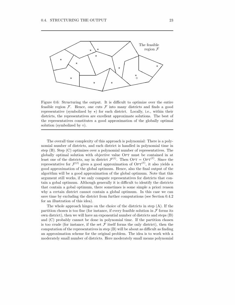
0.4. STRUCTURING THE OUTPUT 23

�� T

TTTaaaaaaa

CCCCCCC

````````````

%%%%%

bbbb!!!!!TTT

�� ZZZ

LLLLLL HH

HH��

llllll

��!!!!

PPPPPCCCCC

,,,,, The feasible

region F

⋆

⋆⋆

⋆

⋆

⋆⋄⋆⋆

⋆

⋆⋆

Figure 0.6: Structuring the output. It is difficult to optimize over the entirefeasible region F . Hence, one cuts F into many districts and finds a goodrepresentative (symbolized by ⋆) for each district. Locally, i.e., within theirdistricts, the representatives are excellent approximate solutions. The best ofthe representatives constitutes a good approximation of the globally optimalsolution (symbolized by ⋄).

The overall time complexity of this approach is polynomial: There is a poly-nomial number of districts, and each district is handled in polynomial time instep (B). Step (C) optimizes over a polynomial number of representatives. Theglobally optimal solution with objective value Opt must be contained in atleast one of the districts, say in district F (ℓ). Then Opt = Opt(ℓ). Since therepresentative for F (ℓ) gives a good approximation of Opt(ℓ), it also yields agood approximation of the global optimum. Hence, also the final output of thealgorithm will be a good approximation of the global optimum. Note that thisargument still works, if we only compute representatives for districts that con-tain a gobal optimum. Although generally it is difficult to identify the districtsthat contain a gobal optimum, there sometimes is some simple a priori reasonwhy a certain district cannot contain a global optimum. In this case we cansave time by excluding the district from further computations (see Section 0.4.2for an illustration of this idea).

The whole approach hinges on the choice of the districts in step (A). If thepartition chosen is too fine (for instance, if every feasible solution in F forms itsown district), then we will have an exponential number of districts and steps (B)and (C) probably cannot be done in polynomial time. If the partition chosenis too crude (for instance, if the set F itself forms the only district), then thecomputation of the representatives in step (B) will be about as difficult as findingan approximation scheme for the original problem. The idea is to work with amoderately small number of districts. Here moderately small means polynomial

24

in the size of the instance I, exactly as required in the statement of step (A).In every district, all the feasible solutions share a certain common property (forinstance, some district may contain all feasible solutions that run the same jobJ11 at time 8 on machine M3). This common property fixes several parametersof the feasible solutions in the district, whereas other parameters are still free.And in the ideal case, it is easy to approximately optimize the remaining freeparameters.

To our knowledge the approach of structuring the output was first usedin 1969 in a paper by Graham [27] on makespan minimization on identicalmachines. Remarkably, in the last section of his paper Graham attributes theapproach to a suggestion by Dan Kleitman and Donald E. Knuth. So it seemsthat this approach has many fathers. Hochbaum & Maass [36] use the approachof structuring the output to get a PTAS for covering a Euclidean point setby the minimum number of unit-squares. In the 1990s, Leslie Hall and DavidShmoys wrote a sequence of very influential papers (see Hall [29, 31], Hall &Shmoys [32, 33, 34]) that all are based on the concept of a so-called outline.An outline is a compact way of specifying the common properties of a set ofschedules that form a district. Hence, approximation schemes based on outlinesfollow the approach of structuring the output.

In the following two sections, we will illustrate the technique of simplifyingthe output with the help of two examples. Section 0.4.1 deals with makespanminimization on two identical machines; we will discuss the arguments of Gra-ham [27]. Section 0.4.2 deals with makespan minimization on two unrelatedmachines. Section 0.4.3 lists several exercises.


The problem. We return to the problem P2 | |Cmax that was introducedand thoroughly discussed in Section 0.3.1: There are n jobs Jj (j = 1, . . . , n)with processing times pj, and the goal is to find a schedule on two identicalmachines that minimizes the makespan. Again, we denote psum =

∑nj=1 pj ,

pmax = maxnj=1 pj , and L = max{ 1

2psum, pmax} with

L ≤ Opt. (0.9)

In this section we will construct another PTAS for P2 | |Cmax, but this time thePTAS will be based on the technique of structuring the output. We will roughlyfollow the argument in the paper of Graham [27] from 1969.

(A) How to define the districts. Let I be an instance of P2 | |Cmax, and letε > 0 be a precision parameter. Recall from Section 0.3.1 that a small job is ajob with processing time at most εL, that a big job is a job with processing timestrictly greater than εL, and that there are at most 2/ε big jobs in I. Considerthe set F of feasible solutions for I. Every feasible solution σ ∈ F specifies anassignment of the n jobs to the two machines.

We define the districts F (1),F (2), . . . according to the assignment of the bigjobs to the two machines: Two feasible solutions σ1 and σ2 lie in the same


district if and only if σ1 assigns every big jobs to the same machine as σ2 does.Note that the assignment of the small jobs remains absolutely free. Since thereare at most 2/ε big jobs, there are at most 22/ε different ways for assigning thesejobs to two machines. Hence, the number of districts in our partition is boundedby a fixed constant whose value is independent of the input size. Perfect! Inorder to make the approach work, we could have afforded that the number ofdistricts grows polynomially with the size of I, but we even manage to get alongwith only a constant number of districts!

(B) How to find good representatives. Consider a fixed district F (ℓ), and

denote by Opt(ℓ) the makespan of the best schedule in this district. In F (ℓ) the

assignments of the big jobs to their machines are fixed, and we denote by B(ℓ)i

(i = 1, 2) the total processing time of big jobs assigned to machine Mi. Clearly,

T := max{B(ℓ)1 , B

(ℓ)2 } ≤ Opt(ℓ). (0.10)

Our goal is to determine in polynomial time some schedule in F (ℓ) withmakespan App(ℓ) ≤ (1+ ε)Opt(ℓ). Only the small items remain to be assigned.Small items behave like sand, and it is easy to pack this sand in a very denseway by sprinkling it across the machines. More formally, we do the following:

The initial workload of machines M1 and M2 are B(ℓ)1 and B

(ℓ)2 , respectively.

We assign the small jobs one by one to the machines; every time a job is as-signed, it is put on the machine with the currently smaller workload (ties are

broken arbitrarily). The resulting schedule σ(ℓ) with makespan App(ℓ) is ourrepresentative for the district F (ℓ). Clearly, σ(ℓ) is computable in polynomialtime.

How close is App(ℓ) to Opt(ℓ)? In case App(ℓ) = T holds, the inequality(0.10) yields that σ(ℓ) in fact is an optimal schedule for the district F (ℓ). In

case App(ℓ) > T holds, we consider the machine Mi with higher workload inthe schedule σ(ℓ). Then the last job that was assigned to M is a small job andthus has processing time at most εL. At the moment when this small job wasassigned to Mi, the workload of Mi was at most 1

2psum. By using (0.9) we getthat

App(ℓ) ≤ 1

2psum + εL ≤ (1 + ε)L ≤ (1 + ε)Opt ≤ (1 + ε)Opt(ℓ).

Hence, in either case the makespan of the representative is at most 1 + ε timesthe optimal makespan in F (ℓ). Since the selection step (C) is trivial to do, weget the PTAS.

Discussion. Let us compare our new PTAS for P2 | |Cmax to the old PTAS forP2 | |Cmax from Section 0.3.1 that was based on the technique of structuring theinput. An obvious similarity is that both approximation schemes classify thejobs into big ones and small ones, and then treat big jobs differently from smalljobs. Another similarity is that the time complexity of both approximationschemes is linear in n, but exponential in 1/ε. But apart from this, the two

26

approaches are very different: The old PTAS manipulates and modifies theinstance I until it becomes trivial to solve, whereas the strategy of the newPTAS is to distinguish lots of cases that all are relatively easy to handle.

0.4.2 Makespan on two unrelated machines

The problem. In the scheduling problem R2 | |Cmax the input consists of twounrelated machines A and B, together with n jobs Jj (j = 1, . . . , n). If job Jj

is assigned to machine A then its processing time is aj , and if it is assigned tomachine B then its processing time is bj. The objective is to find a schedule thatminimizes the makespan. The problem R2 | |Cmax is NP-hard in the ordinarysense. We will construct a PTAS for R2 | |Cmax that uses the technique ofstructuring the output. This section is based on Potts [67].

Let I be an instance of R2 | |Cmax, and let ε > 0 be a precision parameter.We denote K =

∑nj=1 min{aj , bj}, and we observe that

1

2K ≤ Opt ≤ K. (0.11)

To see the lower bound in (0.11), we observe that in the optimal schedule jobJj will run for at least min{aj, bj} time units. Hence, the total processing timein the optimal schedule is at least K and the makespan is at least 1

2K. To seethe upper bound in (0.11), consider the schedule that assigns Jj to machine A ifaj ≤ bj and to machine B if aj > bj . This schedule is feasible, and its makespanis at most K.

(A) How to define the districts. Consider the set F of feasible solutionsfor I. Every feasible solution σ ∈ F specifies an assignment of the n jobs to thetwo machines. A scheduled job in some feasible solution is called big if and onlyif its processing time is greater than εK. Note that this time we define big jobsonly relative to a feasible solution! There is no obvious way of doing an absolutejob classification that is independent of the schedules, since there might be jobswith aj > εK and bj ≤ εK, or jobs with aj ≤ εK and bj > εK. Would onecall such a job big or small? Our definition is a simple way of avoiding thisdifficulty.

The districts are defined according to the assignment of the big jobs to thetwo machines: Two feasible solutions σ1 and σ2 lie in the same district if andonly if σ1 and σ2 process the same big jobs on machine A and the same bigjobs on machine B. For a district F (ℓ), we denote by A(ℓ) the total processingtime of big jobs assigned to machine A, and by B(ℓ) the total processing timeof big jobs assigned to machine B. We kill all districts F (ℓ) for which A(ℓ) > Kor B(ℓ) > K holds, and we disregard them from further consideration. Becauseof inequality (0.11), these districts cannot contain an optimal schedule andhence are worthless for our investigation. Exercise 0.4.4 in Section 0.4.3 evendemonstrates that killing these districts is essential, since otherwise the timecomplexity of the approach might explode and become exponential!


Now let us estimate the number of surviving districts. Since A(ℓ) ≤ K holdsin every surviving district F (ℓ), at most 1/ε big jobs are assigned to machineA. By an analogous argument, at most 1/ε big jobs are assigned to machine B.Hence, the district is fully specified by up to 2/ε big jobs that are chosen froma pool of up to n jobs. This yields O(n2/ε) surviving districts. Since ε is fixedand not part of the input, the number of districts is polynomially bounded inthe size of the input.

(B) How to find good representatives. Consider some surviving districtF (ℓ) in which the assignment of the big jobs has been fixed. The unassignedjobs belong to one of the following four types:

(i) aj ≤ εK and bj ≤ εK,

(ii) aj > εK and bj ≤ εK,

(iii) aj ≤ εK and bj > εK,

(iv) aj > εK and bj > εK.

If there is an unassigned job of type (iv), the district F (ℓ) is empty, and we maydisregard it. If there are unassigned jobs of type (ii) or (iii), then we assign themin the obvious way without producing any additional big jobs. The resultingfixed total processing time on machines A and B is denoted by α(ℓ) and β(ℓ),respectively. We renumber the jobs such that J1, . . . , Jk with k ≤ n become theremaining unassigned jobs. Only jobs of type (i) remain to be assigned, andthis is done by means of the integer linear program (ILP) and its relaxation(LPR) that both are depicted in Figure 0.7: For each job Jj with 1 ≤ j ≤ k,there is a 0-1-variable xj in (ILP) that encodes the assignment of Jk. If xj = 1,then Jj is assigned to machine A, and if xj = 0, then Jj is assigned to machineB. The variable z denotes the makespan of the schedule. The first and secondconstraints state that z is an upper bound on the total processing time on themachines A and B. The remaining constraints in (ILP) are just integralityconstraints. The linear programming relaxation (LPR) is identical to (ILP),except that here the xj are continuous variables in the interval [0, 1].

(ILP ) (LPR)

min z min z

s.t. α(ℓ) +∑k

j=1 ajxj ≤ z s.t. α(ℓ) +∑k

j=1 ajxj ≤ z

β(ℓ) +∑k

j=1 bj(1 − xj) ≤ z β(ℓ) +∑k

j=1 bj(1 − xj) ≤ z

xj ∈ {0, 1} j = 1, . . . , k. 0 ≤ xj ≤ 1 j = 1, . . . , k.

Figure 0.7: The integer linear program (ILP) and its relaxation (LPR) in Sec-tion 0.4.2.

28

The integrality constraints on the xj make it NP-hard to find a feasiblesolution for (ILP). But this does not really matter to us, since the linear pro-gramming relaxation (LPR) is easy to solve! We determine in polynomial timea basic feasible solution x∗

j with j = 1, . . . , n and z∗ for (LPR). Assume thatexactly f of the values x∗

j are fractional, and that the remaing k − f values areintegral. We want to analyze which of the 2k + 2 inequalities of (LPR) maybe fulfilled as an equality by the basic feasible solution: For every integral x∗

j ,equality holds in exactly one of the two inequalities 0 ≤ x∗

j and x∗

j ≤ 1. Forevery fractional x∗

j , equality holds in none of the two inequalities 0 ≤ x∗

j andx∗

j ≤ 1. Moreover, the first two constraints may be fulfilled with equality. Allin all, this yields that at most k − f + 2 of the constraints can be fulfilled withequality. On the other hand, a basic feasible solution is a vertex of the under-lying polyhedron in (k + 1)-dimensional space. It is only determined if equalityholds in at least k + 1 of the 2k + 2 inequalities in (LPR). We conclude thatk + 1 ≤ k − f + 2, which is equivalent to f ≤ 1.

We have shown that at most one of the values x∗

j is not integral. In otherwords, we have almost found a feasible solution for (ILP)! Now it is easy to geta good representative: Each job Jj with x∗

j = 1 is assigned to machine A, eachJj with x∗

j = 0 is assigned to machine B, and if there is a fractional x∗

j then thecorresponding job is assigned to machine A. This increases the total processingtime on A by at most εK. The makespan App(ℓ) of the resulting representativefulfills

App(ℓ) ≤ z∗ + εK ≤ Opt(ℓ) + εK.

Consider a district that contains an optimal solution with makespan Opt. Thenthe makespan of the corresponding representative is at most Opt + εK whichby (0.11) is at most (1 + 2ε)Opt. To summarize, the selection step (C) willfind a representative with makespan at most (1 + 2ε)Opt, and thus we get thePTAS.

0.4.3 Exercises

Exercise 0.4.1. Construct a PTAS for Pm | |Cmax by appropriately modi-fying the approach described in Section 0.4.1. Classify the jobs according toL = max{ 1

mpsum, pmax}, and define the districts according to the assignmentof the big jobs. How many districts do you get? How do you compute goodrepresentatives in polynomial time? What is your worst case guarantee in termsof ε and m? How does your time complexity depend on ε and m?

Can you modify the PTAS from Section 0.4.1 so that it works for the problemP | |Cmax with an arbitrary number of machines? What are the main obstaclesin this approach?

Exercise 0.4.2. This exercise concerns the PTAS for P2 | |Cmax in Sec-tion 0.4.1. Recall that in every district F (ℓ), all the schedules had the same

workloads B(ℓ)1 and B

(ℓ)2 of big jobs on the machines M1 and M2, respectively.

We first computed a representative for every district by greedily adding the


small jobs, and afterwards selected the globally best representative.

(a) Suppose that we mess up these two steps in the following way: First, we

select the district F (ℓ) that minimizes max{B(ℓ)1 , B

(ℓ)2 }. We immediately

abandon all the other districts. Then we compute the representative forthe selected district by greedily adding the small jobs, and finally outputthis representative. Would this still yield a PTAS?

(b) Generalize your answer from (a) to the problem Pm | |Cmax. To do this,you probably should first work your way through Exercise 0.4.1.

Exercise 0.4.3. Consider n jobs Jj (j = 1, . . . , n) with positive integer pro-cessing times pj on three identical machines. The goal is to find a schedule withmachine loads L1, L2, and L3 that minimizes the value L2

1 + L22 + L2

3, i.e., thesum of squared machine loads.

(a) Construct a PTAS for this problem by following the approach describedin Section 0.4.1.

(b) Now consider the messed up approach from Exercise 0.4.2 that first selectsthe ‘best’ district by only judging from the assignment of the big jobs, andafterwards outputs the representative for the selected district. Will thisstill yield a PTAS?

[Hint: For a fixed precision ε, define E = ⌈1/ε⌉. Investigate the instanceI(ε) that consists of six jobs with lengths 13, 9, 9, 6, 6, 6 together with Etiny jobs of length 5/E.]

(c) Does the messed up approach from Exercise 0.4.2 yield a PTAS for mini-mizing the sum of squared machine loads on m = 2 machines?

Exercise 0.4.4. When we defined the districts in Section 0.4.2, we decided tokill all districts F (ℓ) with A(ℓ) > K or B(ℓ) > K. Consider an instance I ofR2 | |Cmax with n jobs, where aj = 0 and bj ≡ b > 0 for 1 ≤ j ≤ n. Howmany districts are there overall? How many of these districts are killed, andhow many of them survive and get representatives?

Exercise 0.4.5. Construct a PTAS for Rm | |Cmax via the approach describedin Section 0.4.2. How do you define your districts? How many districts do youget? How many constraints are there in your integer linear program? What canyou say about the number of fractional values in a basic feasible solution for therelaxation? How do you find the representatives?

Exercise 0.4.6. This exercise deals with problem P3 | pmtn |Rej+Cmax, a vari-ant of parallel machine scheduling with job rejections. An instance consists ofn jobs Jj (j = 1, . . . , n) with a rejection penalty ej and a processing time pj .The goal is to reject a subset of the jobs and to schedule the remaining jobs

30

preemptively on three identical machines, such that the total penalty of all re-jected jobs plus the makespan of the scheduled jobs becomes minimum. Thisproblem is NP-hard in the ordinary sense (Hoogeveen, Skutella & Woeginger[41]). The optimal makespan for preemptive scheduling without rejections isthe maximum of the length of the longest job and of the average machine load;see [55].

Design a PTAS for P3 | pmtn |Rej+Cmax! [Hint: First get upper and lowerestimates on the optimal solution. Define big jobs with respect to these esti-mates. The districts are defined with respect to the rejected big jobs. As inSection 0.4.2, use a linear relaxation of an integer program to schedule the smalljobs in the representatives.]

Exercise 0.4.7. This exercise asks you to construct a PTAS for the followingvariant of the knapsack problem. The input consists of n items with positiveinteger sizes aj (j = 1, . . . , n) and of a knapsack with capacity b. The goal isto pack the knapsack as full as possible but without overpacking it. In otherwords, the goal is to determine J ⊆ {1, . . . , n} such that

∑j∈J aj is maximized

subject to the constraint∑

j∈J aj ≤ b.

(a) Classify items into big ones (those with size greater than εb) and smallones (those with size at most εb). Define your districts via the set ofbig items that a feasible solution packs into the knapsack. What is themaximum number of big items that can fit into the knapsack? How manydistricts do you get?

(b) Explain how to find good representatives for the districts.

Exercise 0.4.8. This exercise asks you to construct a PTAS for the followingproblem. The input consists of n items with positive integer sizes aj (j =1, . . . , n) and of two knapsacks with capacity b. The goal is to pack the maximumnumber of items into the two knapsacks.

(a) Define one special district that contains all feasible packings with up to 2/εitems. The remaining districts are defined according to the placement ofthe big items. How do you define the big items? And how many districtsdo you get?

(b) Explain how you find good representatives for the districts. How do youhandle the special district?

Exercise 0.4.9. All the PTAS’s we have seen so far were heavily based on somea priori upper and lower estimates on the optimal objective value. For instance,in Sections 0.3.1, 0.3.2, and Section 0.4.1 we used the bounds L and 2L on Opt,and in Section 0.4.2 we used the bounds 1

2K and K on Opt, and so on. Thisexercise discusses a general trick for getting a PTAS that works even if you onlyknow very crude upper and lower bounds on the optimal objective value. The

0.5. STRUCTURING THE EXECUTION OF AN ALGORITHM 31

trick demonstrates that you may concentrate on the special situation where youhave an a priori guess x for Opt with Opt ≤ x and where your goals is to finda feasible solution with cost at most (1 + ε)x.

Assume that you want to find an approximate solution for a minimizationproblem with optimal objective value Opt. The optimal objective value itselfis unknown to you, but you know that it is bounded by Tlow ≤ Opt ≤ Tupp.The only tool that you have at your disposal is a black box (this black box isthe PTAS for the special situation described above). If you feed the black boxwith an integer x ≥ Opt, then the black box will give you a feasible solutionwith objective value at most (1 + ε)x. If you feed the black box with an integerx < Opt, then the black box will return a random feasible solution.

How can you use this black to find a globally good approximate solution?How often will you use the black box in terms of Tupp/Tlow? [Hint: Call aninteger x a winner, if the black box returns a feasible solution with cost at most(1 + ε)x, and call it a loser otherwise. Note that every loser x fulfills x < Opt.For k ≥ 0, define xk = (1 + ε)kTlow. Call the black box for the inputs xk untilyou find a winner.]

0.5 Structuring the execution of an algorithm

As third standard approach to the construction of approximation schemes wediscuss the technique of adding structure to the execution of an algorithm. Herethe main idea is to take an exact but slow algorithm A, and to interact withit while it is working. If the algorithm accumulates a lot of auxiliary dataduring its execution, then we may remove part of this data and clean up thealgorithm’s memory. As a result the algorithm becomes faster (since there isless data to process) and generates an incorrect output (since the removal ofdata introduces errors). In the ideal case, the time complexity of the algorithmbecomes polynomial and the incorrect output constitutes a good approximationof the true optimum.

This approach can only work out if the algorithm itself is highly structured.In this chapter we will only deal with rather primitive algorithms that do noteven try to optimize something. They simply generate all feasible solutions andonly suppress obvious duplicates. They are of a severely restricted form andwork in a severely restricted environment. The following two Definitions 0.5.1and 0.5.2 define the type of optimization problem X and the type of algorithmA to which this approach applies.

Definition 0.5.1 (Properties of the optimization problem)

Every instance I of the optimization problem X naturally decomposes inton pieces P1, . . . , Pn. For every k with 1 ≤ k ≤ n, the prefix sequence P1, . . . , Pk

of pieces forms an instance of the optimization problem X. We write Ik shortfor this prefix sequence.

32

The relevant properties of every feasible solution σ of I can be conciselyencoded by a d-dimensional vector ~v(σ) with non-negative coordinates such thatthe following two conditions are satisfied:

(i) The objective value of σ can be deduced in constant time from ~v(σ).

(ii) An algorithm (as described in Definition 0.5.2 below) is able to digest thevectors that encode the feasible solutions for Ik and to deduce from themand from the piece Pk the vectors for all feasible solutions of Ik+1.

This definition is so vague that it needs an immediate illustration. Consideronce again the scheduling problem P2 | |Cmax from Sections 0.3.1 and 0.4.1.The job Jk (k = 1, . . . , n) forms the input piece Pk, and the instance Ik is therestriction of instance I to the first k jobs. The concise encoding of a feasibleschedule σ with machine loads L1 and L2 simply is the two-dimensional vector~v(σ) = [L1, L2]. And the objective value of σ can be deduced from ~v(σ) bytaking the maximum of the two coordinates, as we required in condition (i)above.

Definition 0.5.2 (Properties of the algorithm)

(Initialization). Algorithm A computes in constant time all feasible solutionsfor the instance I1 and puts the corresponding encoding vectors into the vectorset VS1.

(Phases). Algorithm A works in phases. In the k-th phase (k = 2, . . . , n) thealgorithm processes the input piece Pk and generates the vector set VSk. Thisis done as follows. The algorithm takes every possible vector ~v(σ) in VSk−1

and combines the input piece Pk in all possible ways with the underlying feasiblesolution σ. The vectors that encode the resulting feasible solutions form the setVSk. We assume that every single vector in VSk−1 can be handled in constanttime and only generates a constant number of vectors in VSk.

(Output). After the n-th phase, the algorithm computes for every vector inVSn the corresponding objective value and outputs the best solution that it finds.

Note that two distinct feasible solutions σ1 and σ2 with ~v(σ1) = ~v(σ2) areonly stored once in any vector set. Now assume that X is an optimizationproblem as described in Definition 0.5.1 and that A is an algorithm for X asdescribed in Definition 0.5.2. What can we say about the time complexity of A?The initialization step of A needs only constant time. Since every single vectorin VSk−1 is handled in constant time, the time complexity for the k-th phaseis proportional to |VSk−1|. The time complexity for the output step is propor-tional to |VSn|. To summarize, the overall time complexity of A is proportionalto

∑nk=1 |VSk|. In general this value

∑nk=1 |VSk| will be exponential in the size

of the input, and hence algorithm A will not have polynomial time complexity.Let us try to transform algorithm A into an approximation algorithm for

problem X . Note that algorithm A accumulates a lot of intermediate data –all the vector sets VSk – during its execution. We consider the vectors in VSk

as geometric points in d-dimensional Euclidean space. If two of these points


are very close to each other (in the geometric sense) then they should alsoencode very similar feasible solutions. And in this case there is no reason tokeep both of them! We simply remove one of them from the vector set. Bydoing many such removals in an approriate way, we may thin out the vectorsets and (hopefully) bring their cardinalities down to something small. And ifthe cardinalities of all vector sets VSk are small, then the time complexity ofalgorithm A is (polynomially) small, too. And as only feasible solutions wereremoved that had surviving feasible solutions close to them, we probably willget a fairly good approximate solution in the end.

The approach of adding structure to the execution of an algorithm wasintroduced by Ibarra & Kim [44] in 1975. Then Sahni [70] applied it to getan FPTAS for a variety of scheduling problems, and Gens & Levner [25] appliedit to get an FPTAS for minimizing the weighted number of tardy jobs on a singlemachine. In the 1990s, the approach was for instance used in the papers by Potts& Van Wassenhove [68], Kovalyov, Potts & Van Wassenhove [52], and Kovalyov& Kubiak [51]. Woeginger [80] studied the applicability of this approach ina fairly general setting, and he identified several arithmetical and structuralconditions on some underlying cost and transition functions that automaticallyguarantee the existence of an FPTAS. Since the conditions in [80] are verytechnical, we will not discuss them in this tutorial.

In the following four sections, we will illustrate the technique of addingstructure to the execution of an algorithm with the help of four examples. Sec-tion 0.5.1 deals (once again!) with makespan minimization on two identicalmachines, Section 0.5.2 deals with the minimization of the total weighted jobcompletion time on two identical machines, Section 0.5.3 gives an FPTAS forthe knapsack problem, and Section 0.5.4 discusses the weighted number of tardyjobs on a single machine. Section 0.5.5 contains a number of exercises.


The problem. We return once again to the problem P2 | |Cmax that wasalready discussed in Sections 0.3.1 and 0.4.1. Recall that in an instance I ofP2 | |Cmax there are n jobs Jj (j = 1, . . . , n) with processing times pj, and thegoal is to find a schedule on two identical machines M1 and M2 that minimizesthe makespan. Denote psum =

∑nj=1 pj . Observe that the size |I| of the input

I satisfies

|I| ≥ log(psum) = const · ln(psum). (0.12)

Just to write down all the values pj in binary representation we need log(psum)bits! We note that the exact value of the constant in (0.12) equals log(e) wheree is the base of the natural logarithm. For our purposes it is sufficient to knowthat it is some positive number that does not depend on the instance I. In thissection, we will find a third approximation scheme for P2 | |Cmax. This time,we will find an FPTAS whereas the approximation schemes in Sections 0.3.1and 0.4.1 only were PTAS’s.

34

We encode a feasible schedule σ with machine loads L1 and L2 by the two-dimensional vector [L1, L2]. Condition (i) in Definition 0.5.1 is trivially fulfilled,since the objective value of the encoded schedule σ equals max{L1, L2}. Con-dition (ii) goes hand in hand with the algorithm A from Definition 0.5.2.

Initialization. Set VS1 = {[p1, 0], [0, p1]}.Phase k. For every vector [x, y] in VSk−1, put [x + pk, y] and[x, y + pk] in VSk.

Output. Output the vector [x, y] ∈ VSn that minimizes the valuemax{x, y}.

Since the coordinates of all vectors in all sets VSk are integers in the rangefrom 0 to psum, the cardinality of every vector set VSk is bounded fromabove by O(p2

sum). Since the time complexity of the algorithm is propor-tional to

∑nk=1 |VSk|, the algorithm has a pseudo-polynomial time complexity

of O(n p2sum).

How to simplify the vector sets. All considered vectors correspond togeometric points in the rectangle [0, psum]×[0, psum]. We subdivide this rectanglewith horizontal and vertical cuts into lots of boxes; in both directions these cutsare made at the coordinates ∆i for i = 1, 2, . . . , L where

∆ = 1 +ε

2n. (0.13)

and where

L = ⌈log∆(psum)⌉ = ⌈ln(psum)/ ln(∆)⌉ ≤ ⌈(1 +2n

ε) ln(psum)⌉. (0.14)

The last inequality holds since for all z ≥ 1 we have ln z ≥ (z − 1)/z (which canbe seen from the Taylor expansion of ln z). If two vectors [x1, y1] and [x2, y2]fall into the same box of this subdivision, then their coordinates satisfy

x1/∆ ≤ x2 ≤ x1 ∆ and y1/∆ ≤ y2 ≤ y1 ∆. (0.15)

Since ∆ is very small, vectors in the same box indeed are very close to eachother. Now it is straightforward to simplify the vector set VSk: Out of everybox that has non-empty intersection with VSk we select a single vector and putit into the so-called trimmed vector set VS#

k . All remaining vectors from thevector set VSk that have not been selected are lost for the further computations.And in phase k + 1, the so-called trimmed algorithm generates its new vectorset from the smaller set VS#

k , and not from the set VSk. What can be said

about the resulting time complexity? The trimmed vector set VS#k contains at

most one vector from each box in the subdivision. Altogether there are O(L2)boxes, and so by (0.14) and by (0.12) the number of boxes is polynomial in theinput size |I| and also polynomial in 1/ε. And since the time complexity of the

trimmed algorithm is proportional to∑n

k=1 |VS#k |, the trimmed algorithm has

a time complexity that is polynomial in the input size and in 1/ε.


How to analyze the worst case behavior. The original (untrimmed) algo-rithm works with vector sets VS1, . . . ,VSn where VSk+1 is always computedfrom VSk. The trimmed algorithm works with vector sets VS#

1 , . . . ,VS#n where

VS#k+1 is always computed from VS#

k . We will prove the following statement

by induction on k that essentially says that the vector set VS#k is a decent ap-

proximation of the vector set VSk: For every vector [x, y] ∈ VSk there exists a

vector [x#, y#] in VS#k such that

x# ≤ ∆k x and y# ≤ ∆k y. (0.16)

Indeed, for k = 1 the statement follows from the inequalities in (0.15). Nowassume that the statement holds true up to some index k − 1, and consideran arbitrary vector [x, y] ∈ VSk. The untrimmed algorithm puts this vectorinto VSk when it adds job Jk to some feasible schedule for the first k − 1jobs. This feasible schedule for the first k − 1 jobs is encoded by a vector[a, b] ∈ VSk−1, and either [x, y] = [a + pk, b] or [x, y] = [a, b + pk] must hold.Since both cases are completely symmetric, we assume without loss of generalitythat [x, y] = [a + pk, b]. By the inductive assumption, there exists a vector

[a#, b#] in VS#k−1 with

a# ≤ ∆k−1 a and b# ≤ ∆k−1 b. (0.17)

The trimmed algorithm generates the vector [a# + pk, b#] in the k-th phase.The trimming step may remove this vector again, but it must leave some vector[α, β] in VS#

k that is in the same box as [a# + pk, b#]. Now we are done. Thisvector [α, β] is an excellent approximation of [x, y] ∈ VSk in the sense of (0.16).Indeed, its first coordinate α satisfies

α ≤ ∆(a# + pk) ≤ ∆k a + ∆ pk ≤ ∆k(a + pk) = ∆kx.

For the first inequality, we used that [α, β] and [a#+pk, b#] are in the same box,and for the second inequality, we used (0.17). By analogous arguments, we canshow that β ≤ ∆ky, and this completes the inductive proof. This proof lookssomewhat technical, but its essence is very simple: The untrimmed algorithmand the trimmed algorithm roughly run in parallel and always perform roughlyparallel actions on perturbed versions of the same data.

At the very end of its execution, the untrimmed algorithm outputs thatvector [x, y] in VSn that minimizes the value max{x, y}. By our inductiveproof there is a vector [x#, y#] in VS#

n whose coordinates are at most a factorof ∆n above the corresponding coordinates of [x, y]. We conclude that

max{x#, y#} ≤ max{∆n x, ∆n y} = ∆n max{x, y} = ∆nOpt,

and that our algorithm is a ∆n-approximation algorithm for P2 | |Cmax. Howlarge is ∆n? In (0.13) we defined ∆ = 1+ ε

2n . A well-known inequality says that(1+z/n)n ≤ 1+2z holds for 0 ≤ z ≤ 1 (The left-hand side of this inequality is aconvex function in z, and its right-hand side is a linear function in z. Moreover,

36

the inequality holds true at the two endpoints z = 0 and z = 1). By settingz = ε/2 in this inequality, we get that ∆n ≤ 1+ε. So we indeed have constructedan FPTAS!

Discussion. What are the special properties of problem P2 | |Cmax and of theuntrimmed algorithm that make this approach go through? Well, to get the timecomplexity down to polynomial we made heavy use of the fact that the lengthsof the sides of the rectangle [0, psum] × [0, psum] grow at most exponentiallywith the input size. The variable L defined in (0.14) depends logarithmicallyon these sidelengths, and the final time complexity of the trimmed algorithmdepends polynomially on L. So, one necessary property is that the coordinatesof all vectors in the vector sets are exponentially bounded in |I|. The numberof boxes is roughly Ld where d is the dimension of the vectors. Hence, it isimportant that this dimension is a fixed constant and does not depend on theinput.

The inductive argument in our analysis of the worst case behavior is basedon fairly general ideas. One way of looking at the algorithm is that it translatesold vectors for the instance Ik−1 into new vectors for the instance Ik. Thetwo translation functions are F1[x, y] = [x + pk, y] and F2[x, y] = [x, y + pk].The coordinates of the new vectors are non-negative linear combinations of thecoordinates of the old vectors, and in fact that is the crucial property that makesthe inductive argument go through; see Exercise 0.5.2 in Section 0.5.5.

In the final step, the algorithm extracts the optimal objective value fromthe final vector set. This corresponds to another function G[x, y] = max{x, y}that translates vectors into numbers. Here the crucial property is that the valueG[(1+ε)x, (1+ε)y] is always relatively close to the value G[x, y]. This propertyis crucial, but also fairly weak. It is fulfilled by most natural and by manyunnatural objective functions. The reader may want to verify that for instancethe function G[x, y] = x3 + max{4x, y2} also satisfies this property. For a moregeneral discussion and a better view on this approach we refer to Woeginger[80].

0.5.2 Total weighted job completion time on two identical

machines

The problem. In the scheduling problem P2 | | ∑wjCj the input consists of

n jobs Jj (j = 1, . . . , n) with positive integer processing times pj and positiveinteger weights wj . All jobs are available for processing at time 0, and the goalis to schedule them on two identical machines such that the weighted sum of jobcompletion times is minimized. Denote psum =

∑nj=1 pj and wsum =

∑nj=1 wj ,

and observe that the size |I| of the input I is at least log(psum) + log(wsum).The problem P2 | | ∑

wjCj is NP-hard in the ordinary sense (Bruno, Coffman& Sethi [16]). In this section we describe an FPTAS for P2 | | ∑

wjCj that usesthe technique of adding structure to the execution of an algorithm. We willroughly follow the ideas of Sahni [70].


The solution. We first renumber the jobs such that p1/w1 ≤ p2/w2 ≤ · · · ≤pn/wn holds. A simple job interchange argument (see for instance [55]) showsthat there always exists an optimal schedule which does not contain any idletime, and in which both machines process the jobs in increasing order of index.We encode a feasible schedule σ by a 3-dimensional vector [L1, L2, Z]: The firstcoordinate L1 is the total load of σ on the first machine, the second coordinateL2 is the total load on the second machine, and the third coordinate Z is theweighted sum of job completion times in σ. Our untrimmed algorithm A nowlooks as follows.

Initialization. Set VS1 = {[p1, 0, p1w1], [0, p1, p1w1]}.Phase k. For every vector [x, y, z] in VSk−1, put the vectors [x +pk, y, z + wk(x + pk)] and [x, y + pk, z + wk(y + pk)] in VSk.

Output. Output the vector [x, y, z] ∈ VSn that minimizes the zvalue.

In the k-th phase, the algorithm schedules job Jk at the end of the first machinewhich increases the machine load by pk and the objective value by wk(x +pk), and it schedules Jk at the end of the second machine which increases themachine load by pk and the objective value by wk(y + pk). If one comparesthis algorithm to the algorithm in Section 0.5.1 then one realizes that thereare many similarities between the two of them. In fact, the definition of thetrimmed algorithm and the analysis of its worst case behavior can be cariedout almost analogously to Section 0.5.1. Therefore, we will only briefly indicatethat all the properties are fulfilled that took shape in the discussion at the endof Section 0.5.1.

The first two coordinates of all vectors in all sets VSk are integers in therange from 0 to psum, and the third coordinate is an integer in the range from0 to psumwsum. The coordinates of all vectors in the vector sets are exponen-tially bounded in |I|, exactly as we required in the discussion at the end ofSection 0.5.1. There are two translation functions that translate old vectors forthe instance Ik−1 into new vectors for the instance Ik, and in both of them thecoordinates of the new vectors are non-negative linear combinations of the co-ordinates of the old vectors. That is all we need for an inductive proof that thevector set VS#

k is a good approximation of the vector set VSk, see Exercise 0.5.2in Section 0.5.5. Finally, the objective value is extracted from a vector [x, y, z]by the projection G[x, y, z] = z. If the values x, y, and z are perturbed by atmost a factor of 1 + ε, then the value of the projection is increased by at mosta factor of 1 + ε. Hence, we indeed have all the ingredients that are needed tomake the approach go through. This yields the FPTAS.

0.5.3 The knapsack problem

The problem. In the 0/1-knapsack problem an instance I consists of n itemswith profits pj and weights wj (j = 1, . . . , n), together with a weight bound W .All numbers in the data are non-negative integers. The goal is to select a subset

38

of the items whose total weight does not exceed the weight bound W such thatthe total profit of the selected items is maximized. Denote psum =

∑nj=1 pj and

wsum =∑n

j=1 wj ; the size |I| is at least log(psum)+log(wsum). The 0/1-knapsackproblem is NP-hard in the ordinary sense (Karp [48]). The first FPTAS for 0/1-knapsack is due to Ibarra & Kim [44]. We present an FPTAS for 0/1-knapsackthat uses the technique of adding structure to the execution of an algorithm.

The solution. We encode a subset of the items by a two-dimensional vector[ω, π]: The first coordinate ω is the total selected weight, and the second coor-dinate π is the total selected profit. Consider the following algorithm for the0/1-knapsack problem in the framework of Definition 0.5.2.

Initialization. If w1 ≤ W then set VS1 = {[w1, p1], [0, 0]}. And ifw1 > W then set VS1 = {[0, 0]}.Phase k. For every vector [x, y] in VSk−1 do the following. Put[x, y] into VSk. If x + wk ≤ W then put [x + wk, y + pk] in VSk.

Output. Output the vector [x, y] ∈ VSn that maximizes the yvalue.

This algorithm is based on the standard dynamic programming formulationof the 0/1-knapsack (Bellman & Dreyfus [15]). It looks fairly similar to thealgorithms we discussed in Sections 0.5.1 and 0.5.2. However, there is a fun-damental difference: If-statements. The algorithms in Sections 0.5.1 and 0.5.2treated all vectors in all vector sets exactly the same way. They translated theold vectors unconditionally into new vectors. The above if-statements, however,treat different vectors in a different way, and that makes the computation of thevector sets less robust. But let us start with the properties that can be carriedover to our situation without any effort. The first coordinates of all vectors areintegers in the range from 0 to wsum, and the second coordinates are integers inthe range from 0 to psum. Hence, both coordinates are exponentially boundedin |I|, exactly as is needed. There are two translation functions that translateold vectors for the instance Ik−1 into new vectors for the instance Ik. In both ofthem the coordinates of the new vectors are non-negative linear combinationsof the coordinates of the old vectors, exactly as we need. The objective value isextracted from a vector [x, y] by the projection G[x, y] = y. If the values x andy are perturbed by at most a factor of 1 + ε, then the value of the projectionis increased by at most a factor of 1 + ε, exactly as we need. So — it seemsthat we have everything exactly as we need to make the approach go through.Where is the problem?

The problem is that the inductive proof showing that VS#k is a good ap-

proximation of VSk does not go through. Read the inductive argument in Sec-tion 0.5.1 again. In a nutshell, this inductive argument finds for any vector ~v inVSk a ∆k-approximation ~v# ∈ VS#

k in the following way. The vector ~v resultsfrom a vector ~u ∈ VSk by a certain translation τ . By the inductive assumption,this vector ~u has a ∆k−1-approximation ~u# ∈ VS#

k−1 which can be translated


by the same translation τ into a vector ~z#. In the end, the vector that is se-lected from the same box as ~z# for VS#

k yields the desired ∆k-approximationfor ~v. Done. The trouble, however, is that the vector ~z# itself might be in-feasible. Then the if-statement weeds out ~z# immediately and the argumentbreaks down. We stress that this problem is not only a technicality of the proof,but in fact it may cause disastrous worst case behavior; see Exercise 0.5.9 inSection 0.5.5. How can we rescue our approach? All the trouble originates frominfeasibilities. So, during the trimming maybe we should not take an arbitraryvector from every box, but should always select the vector that is furthest fromcausing infeasibility? And the vectors that are furthest from causing infeasibil-ity are of course the vectors with the smallest x-coordinates! This indeed worksout. The new trimming step becomes the following:

From every box that intersects the untrimmed vector set, select a sin-gle vector with minimum x-coordinate and put it into the trimmedvector set VS#

k .

And the new inductive statement becomes the following:

For every vector [x, y] in the vector set VSk of the untrimmed algo-

rithm, there exists a vector [x#, y#] in VS#k such that x# ≤ x and

y# ≤ ∆k y.

Note that the main difference to the old inductive statement in (0.16) is thatnow we have the strong inequality x# ≤ x instead of the weaker x# ≤ ∆k x.The inductive proof is fairly easy and is left to the reader, see Exercise 0.5.10in Section 0.5.5.

Discussion. What are the special properties of the knapsack problem thatmake this modified approach go through? As a rule of thumb, the approach goesthrough as long as the region of feasible vectors [x1, . . . , xd] forms a halfspace of

IRd whose bounding hyperplane is of the form∑d

i=1 aixi ≤ A with non-negativereal numbers ai and A. For instance in the knapsack problem above, the feasibleregion is specified by the inequality x ≤ W −wk which clearly satisfies this ruleof thumb. The bounding hyperplane guides us in selecting the vectors thatare furthest from causing infeasibility: From every box we select the vectorthat is furthest from the hyperplane. And this often makes the inductive proofgo through (we note also that the non-negativity of the coefficients ai of thehyperplane is usually needed in the inductive argument). Exercise 0.5.11 inSection 0.5.5 gives an illustration for this.

On the other hand, as soon as the feasible region is of a more complicatedform, then in general there is no hope of getting the approach to go through.There is no simple way to identify the most promising feasible solution in abox. Consider for instance vectors [x, y] in two-dimensional space whose feasibleregion is specified by x ≤ 20 and y ≤ 20. If a box contains the two vectors [9, 11]and [10, 10], which of them shall we put into the trimmed vector set? Eitherchoice may lead to a catastrophy.

40

0.5.4 Weighted number of tardy jobs on a single machine

The problem. In the scheduling problem 1 | | ∑wjUj the input consists of n

jobs Jj (j = 1, . . . , n) with processing times pj , weights wj , and due dates dj . Alljobs are available for processing at time 0. In some schedule a job is called earlyif its processing is completed by its deadline, and otherwise it is called tardy.The goal is to schedule the jobs on a single machine such that the total weightof the tardy jobs is minimized. Denote psum =

∑nj=1 pj and wsum =

∑nj=1 wj ;

the size |I| is at least log(psum)+log(wsum). Problem 1 | | ∑wjUj is NP-hard in

the ordinary sense (Karp [48]). The first FPTAS for 1 | | ∑wjUj is due to Gens

& Levner [25]. We present an FPTAS for 1 | | ∑wjUj that uses the technique

of adding structure to the execution of an algorithm.

The solution. We renumber the jobs such that d1 ≤ d2 ≤ · · · ≤ dn. Underthis numbering, there always exists an optimal schedule in which all early jobsare processed before all tardy jobs and in which all early jobs are processedin increasing order of index. We encode feasible schedules by two-dimensionalvectors [P, W ]: The first coordinate P is the total processing time of the sched-uled early jobs, and the second coordinate W is the total weight of the tardyjobs (that all are shifted far to the future). Consider the following algorithm for1 | | ∑

wjUj in the framework of Definition 0.5.2.

Initialization. If p1 ≤ d1 then set VS1 = {[p1, 0], [0, w1]}. And ifp1 > d1 then set VS1 = {[0, w1]}.Phase k. For every vector [x, y] in VSk−1 do the following. Put[x, y + wk] into VSk. If x + pk ≤ dk then put [x + pk, y] in VSk.

Output. Output the vector [x, y] ∈ VSn that minimizes the yvalue.

This algorithm is based on the dynamic programming formulation of Lawler &Moore [56]. In the k-th phase, the algorithm first schedules job Jk tardy whichincreases the objective value y by wk. Then it tries to schedule Jk early whichincreases the total processing time of the early jobs to x+pk and only is possibleif this value does not exceed the due date dk.

The first coordinates of the vectors are bounded by psum, and their sec-ond coordinates are bounded by wsum. In the two translation functions thattranslate old vectors for the instance Ik−1 into new vectors for the instance Ik,the coordinates of the new vectors are non-negative linear combinations of thecoordinates of the old vectors. The objective value is extracted from a vector[x, y] by the same projection G[x, y] = y as in the knapsack algorithm in Sec-tion 0.5.3. What about if-statements and infeasibilities? Only the x-coordinatecan cause infeasibilities, and so we may always select a vector with minimumx-coordinate from any box and put it into the trimmed vector set VS#

k . Hence,the same machinery as in the preceding sections and the same inductive proofas in Section 0.5.3 will yield the FPTAS.


0.5.5 Exercises

Exercise 0.5.1. When we discussed the general framework at the beginningof Section 0.5, we required in Definition 0.5.1 that extracting the correspondingobjective value from a vector only takes constant time. Moreover, in Defini-tion 0.5.2 we required that the initialization can be done in constant time, andwe required that every fixed vector in VSk−1 only generates a constant numberof vectors in VSk.

Would the approach break down, if we replace the word ‘constant’ by theword ‘polynomial’? Are these restrictions necessary at all?

Exercise 0.5.2. Let X be an optimization problem X as described in Defini-tion 0.5.1, and let A be an algorithm for X as described in Definition 0.5.2. Thefeasible solutions are encoded by d-dimensional vectors. The algorithm gener-ates the vector set VSk by applying the functions F1, . . . , Fq to every vector in

VSk−1. Every Fi (1 ≤ i ≤ q) is a linear function from IRd → IRd, and all the co-ordinates of the images are non-negative linear combinations of the coordinatesof the preimages. The coefficients of these non-negative linear combinationsmay depend on the input piece Pk, but they must remain non-negative. Weperform the trimming of the vector sets as in Section 0.5.1.

Prove that under these conditions, for every vector ~v in VSk there existsa vector ~v# in VS#

k whose coordinates are at most a factor of ∆k above thecorresponding coordinates of ~v. [Hint: Translate the proof from Section 0.5.1to the more general situation.]

Exercise 0.5.3. Construct an FPTAS for Pm | |Cmax by appropriately modi-fying the approach described in Section 0.5.1. How do you encode the feasibleschedules as vectors? What is the dimension of these vectors? How does theworst case guarantee depend on ε and m? How does the time complexity dependon ε and m? Can you extend this approach to get an approximation scheme forP | |Cmax?

Exercise 0.5.4. Consider n jobs Jj (j = 1, . . . , n) with positive integer pro-cessing times pj on three identical machines. The goal is to find a schedule withmachine loads L1, L2, and L3 that minimizes the value L2

1 + L22 + L2

3, i.e., thesum of squared machine loads.

Construct an FPTAS for this problem by following the approach describedin Section 0.5.1. Can you generalize this FPTAS to any fixed number m ofmachines?

Exercise 0.5.5. Construct an FPTAS for R2 | |Cmax, i.e., makespan mini-mization on two unrelated machines (see Section 0.4.2). What are the maindifferences between this FPTAS and the FPTAS for makespan minimization ontwo identical machines described in Section 0.5.1? Can you extend this approachto get an FPTAS for Rm | |Cmax?

42

Exercise 0.5.6. Generalize the FPTAS in Section 0.5.2 to Pm | | ∑wjCj with

a fixed number of machines. How does the dimension of the vectors that encodethe schedules depend on m? Can you extend the approach to P | | ∑

wjCj?Can you extend the approach to R2 | | ∑

wjCj? And to Rm | | ∑wjCj? What

about R | | ∑wjCj?

Exercise 0.5.7. Consider n jobs Jj (J = 1, . . . , n) with processing times pj

on two identical machines. The goal is to find a schedule that minimizes thesum of squared job completion times. Design an FPTAS for this problem bymodifying the arguments from Section 0.5.2. Can you also handle the variantwhere the goal is to minimize the sum of cubed job completion times?

Exercise 0.5.8. Section 0.5.2 discussed the problem of minimizing the sum ofweighted job completion times on two identical machines. This exercise asksyou to find an FPTAS for the problem of minimizing the sum of weighted jobstarting times on two identical machines. How do you order the jobs in thebeginning?

Exercise 0.5.9. Assume that we apply the technique of adding structure to theexecution of an algorithm to the knapsack problem as discussed in Section 0.5.3.Assume that in the trimming we select an arbitrary vector from every box anddo not care about critical coordinates.

Construct knapsack instances for which the worst case ratio of this approachmay become arbitrarily close to 2. [Hint: Use three items that all have roughlythe same profit. Choose the weight w1 very close to the weight bound W , andchoose the weight w2 even closer to W . Choose w3 such that the first andthird item together from a feasible solution, whereas the second and third itemtogether are not feasible. Make the trimming select the ‘wrong’ vector for VS#

2 .]

Exercise 0.5.10. In Section 0.5.3 we designed a new trimming step forthe knapsack problem that from every box selects a vector with minimumx-coordinate for VS#

k . Prove that the resulting algorithm throughout ful-fills the following statement: For every vector [x, y] ∈ VSk there is a vector

[x#, y#] ∈ VS#k with x# ≤ x and y# ≤ ∆k y. [Hint: Follow the inductive

argument in Section 0.5.1.]

Exercise 0.5.11. Consider non-negative integers aj and bj (j = 1, . . . , n), anda non-negative integer C. For a subset K ⊆ {1, . . . , n} denote AK =

∑j∈K aj

and BK =∑

j∈K bj. The goal is to find an index set K with AK + BK ≤ C

such that A2K + B2

K is maximized.

Design an FPTAS for this problem. Encode a feasible subset K by the vector[AK , BK ], and use the approach that is implicit in the discussion at the end ofSection 0.5.3.

Exercise 0.5.12. Consider n items with profits pj and weights wj (j =1, . . . , n), together with a weight bound W . The goal is to fill two knapsacks

0.6. HOW TO GET NEGATIVE RESULTS 43

of capacity W with the items such that the total profit of the packed items ismaximized.

Can you get an FPTAS for this problem by modifying the approach in Sec-tion 0.5.3? What is the main obstacle? Check your thoughts against Exer-cise 0.6.4 in Section 0.6.5.

Exercise 0.5.13. In Section 0.5.4 we described an FPTAS for minimizing thetotal weight of the tardy jobs on a single machine. This exercise deals withthe dual problem of maximizing the total weight of the early jobs on a singlemachine. We use the notation from Section 0.5.4.

(a) Suppose that we call the FPTAS from Section 0.5.4 for the minimizationproblem, and then use the resulting schedule as an approximation for themaximization problem. Explain why this will not yield an FPTAS for themaximization problem.

(b) Design an FPTAS for maximizing the total weight of the early jobs on asingle machine.

Exercise 0.5.14. This exercise asks you to construct an FPTAS for the follow-ing scheduling problem 1 | |Rej+

∑Cj with job rejections. An instance consists

of n jobs Jj (j = 1, . . . , n) with a rejection penalty ej and a processing time pj .The goal is to reject a subset of the jobs and to schedule the remaining jobs ona single machine, such that the total penalty of all rejected jobs plus the sumof completion times of the scheduled jobs becomes minimum. This problem isNP-hard in the ordinary sense (Engels, Karger, Kolliopoulos, Sengupta, Uma& Wein [19]).

How do you get an FPTAS via the technique of adding structure to theexecution of an algorithm? How do you encode the feasible schedules as vectors?What is the dimension of these vectors? [Hint: The problem variant withoutrejections is solved to optimality by scheduling the jobs in the order of non-decreasing lengths. This is a special case of Smith’s ratio rule [75]. It is a goodidea to first bring the jobs into this ordering, and then to go through them andto decide about rejections one by one. Then you only need to know the currenttotal size of all scheduled jobs and the current objective value.]

0.6 How to get negative results

In the previous sections we have concentrated on positive results, and we havelearnt how to construct approximation schemes. In this section we will focus onnegative results, that is, we discuss in-approximability techniques for showingthat a specific problem does not have a PTAS or an FPTAS unless P=NP. Weremind the reader that throughout this chapter we only consider optimizationproblems in which all feasible solutions have non-negative cost.

44

Assume that we want to prove that some optimization problem X is hard toapproximate. The first step in proving an in-approximability result always is tocheck through the web-compendium of Crescenzi & Kann [17] that contains anenormous list of references and results on in-approximability. At least, we willfind out whether problem X is already known to be hard to approximate. If wedo not find problem X in the compendium, then we will have to find our ownin-approximability proof. The structure of an in-approximability proof usuallyis along the following line of argument:

Suppose that there is a good approximability result for problem X .Then some intermediate problem Z1 must have a good algorithm.Then some intermediate problem Z2 must have a good algorithm. . . . . . . . . Then some intermediate problem Zk−1 must have a goodalgorithm. Then the problem Zk that is already known to be hardmust have a good algorithm. Then P=NP.

The intermediate steps usually consist of classical polynomial time reductionsbetween decision problems or by approximation preserving reductions betweenoptimization problems. The number of intermediate problems Z1, . . . , Zk mayvary, but the goal is to eventually reach the conclusion P=NP. Since P=NP isvery unlikely to be true, it is also very unlikely that the starting assumption onthe good approximability result for problem X is true. Hence, if in this sectionwe talk about in-approximability and non-existence of some good algorithm,then we will always mean in-approximability and non-existence of some goodalgorithm under the assumption that P6=NP.

In the following four sections, we will illustrate some standard techniquesfor proving in-approximability results. Section 0.6.1 deals with disproving theexistence of an FPTAS. Here the intermediate problem Z1 is a strongly NP-hardproblem, and in the first intermediate step we deduce the existence of a pseudo-polynomial algorithm for Z1. Section 0.6.2 deals with disproving the existenceof a PTAS by applying the gap technique. Here the intermediate problem Z1

is an NP-hard problem, and in the first intermediate step we deduce the exis-tence of a polynomial algorithm for Z1. Section 0.6.3 deals with disproving theexistence of a PTAS via APX-hardness arguments. Here the intermediate prob-lems Z1, . . . , Zk are already known to be APX-hard, and the intermediate stepsare approximation-preserving reductions from problem Zi+1 to problem Zi. Toprove the in-approximability of X , one only needs to establish an L-reductionfrom Z1 to X ; the remaining intermediate steps are proved in the literature.Section 0.6.4 discusses an example for an L-reduction. Finally, Section 0.6.5contains a long list of exercises.

0.6.1 How to show that there is no FPTAS

The main tool for disproving the existence of an FPTAS for some optimizationproblem is to establish its strong NP-hardness. Strongly NP-hard problems(that fulfill some weak and natural supplementary condition) cannot have anFPTAS unless P=NP, or equivalently, every well-behaved problem that has an


FPTAS is solvable in pseudo-polynomial time. This is a surprising connectionbetween seemingly unrelated concepts, and we want to discuss it in some detail.Let us start by considering the specific example P | |Cmax; we have studied thisproblem already in Section 0.3.2 where we designed a PTAS for it.

Example 0.6.1 An instance I of P | |Cmax is specified by the positive integerprocessing times pj (j = 1, . . . , n) of n jobs together with the number m of iden-tical machines. The goal is to find a schedule that minimizes the makespan. Thisproblem is NP-hard in the strong sense (Garey & Johnson [24]), and thereforethe problem remains NP-hard even if all numbers in the input are encoded inunary.

One possible way of encoding an instance of P | |Cmax in unary is to firstwrite the value m in unary followed by the symbol #, followed by the list of joblengths in unary with the symbol $ as a separation marker. Denote by psum =∑n

j=1 pj the total job processing time. Then the length |I|unary of an instanceI under this unary encoding equals psum + m + n. The instance I that consistsof m = 3 machines together with six jobs with lengths p1 = 1, p2 = 5, p3 = 2,p4 = 6, p5 = 1, p6 = 8 (these numbers are written in decimal representation) isthen encoded as the string 111#1$11111$11$111111$1$11111111.

Throughout the next few paragraphs we will use the notation |I|unary and|I|binary so that we can clearly distinguish between unary and binary encod-ings of an instance. Now consider problem P | |Cmax in the standard binaryencoding where the size of instance I is |I|binary, and suppose that this problemhas an FPTAS. The time complexity of this FPTAS is bounded from above byan expression |I|sbinary/εt where s and t are fixed positive integers. Consider thealgorithm A for P | |Cmax that results from calling the FPTAS for an instance Iwith precision ε = 1/(psum +1). What is the time complexity of this algorithm,and how close does algorithm A come to the optimal objective value? The timecomplexity of algorithm A is bounded from above by |I|sbinary · (psum +1)t which

in turn is bounded by O(|I|s+tunary). Hence, A is a pseudo-polynomial algorithm

for P | |Cmax. Next we claim that algorithm A always finds an optimal solutionfor instance I. Otherwise, we would have

Opt(I) + 1 ≤ A(I) ≤ (1 + ε)Opt(I) = (1 +1

psum + 1)Opt(I).

Here the first inequality follows from the fact that all possible objective val-ues are integers, and the other inequality follows by the chosen precision ofapproximation. The displayed inequality implies Opt(I) ≥ psum + 1 which isblatantly wrong; even the trivial schedule that assigns all the jobs to the samemachine has makespan at most psum. Hence, algorithm A outputs an optimalsolution. To summarize, if there is an FPTAS for P | |Cmax then there is apseudo-polynomial algorithm A for P | |Cmax. And since P | |Cmax is stronglyNP-hard, the existence of a pseudo-polynomial algorithm for this problem im-plies P=NP. In other words, unless P=NP problem P | |Cmax cannot have anFPTAS.

46

The above argument is fairly general. It only exploits the fact that allpossible objective values are integral, and the fact that Opt ≤ psum. Theargument easily generalizes to the following well-known theorem of Garey &Johnson [23]; see Exercise 0.6.1 in Section 0.6.5 for a sketch of its proof.

Theorem 0.6.2 (Well-behaved and strongly NP-hard =⇒ no FPTAS)Let X be a strongly NP-hard minimization or maximization problem that satis-fies the following two conditions:

(i) All feasible solutions of all instances I have integral costs.

(ii) There exists a polynomial p such that Opt(I) ≤ p(|I|unary) holds for allinstances I.

Then the optimization problem X does not have an FPTAS unless P=NP.

Note that the conditions (i) and (ii) in this theorem are not very restrictive, andare fulfilled by most natural optimization problems (and see Exercise 0.6.2 inSection 0.6.5 for some optimization problems that are less natural and do notfulfill these conditions). In other words, every well-behaved problem with an FP-TAS is pseudo-polynomially solvable! What about the reverse statement? Doesevery well-behaved pseudo-polynomially solvable problem have an FPTAS? Theanswer to this question is no, and it actually is quite easy to construct (somewhatartificial) counter-examples that are pseudo-polynomially solvable problems butdo not have an FPTAS; see for example Exercise 0.6.3 in Section 0.6.5. Whatwe are going to do next is to discuss a quite natural counter-example with theseproperties.

Example 0.6.3 (Korte & Schrader [50])Consider the following two-dimensional variant of the knapsack problem: Thereare n items with positive integer weights wj and positive integer volumes vj

(j = 1, . . . , n), and there is a knapsack with a weight capacity W and a volumecapacity V . The goal is to pack the maximum number of items into the knapsackwithout exceeding the weight and volume limits.

Although this two-dimensional knapsack problem is easily solved in pseudo-polynomial time, it does not have an FPTAS unless P=NP.

The proof is done by a reduction from the following partition problem that isNP-hard in the ordinary sense: The input to the partition problem consists of2m positive integers a1, . . . , a2m that sum up to 2A and that fulfill A/(m+1) <ak < A/(m − 1) for k = 1, . . . , 2m. The problem is to decide whether thereexists an index set K such that

∑k∈K ak = A holds. From an instance of

the partition problem, we now define the following instance of the knapsackproblem with n = 2m items: For k = 1, . . . , 2m, item k has weight wk = ak andvolume vk = A − ak. The weight bound is W = A, and the volume bound isV = (m − 1)A.

Now suppose that the two-dimensional knapsack problem does possess anFPTAS. Set ε = 1

2m and call the FPTAS for the constructed two-dimensional


knapsack instance. Note that the resulting time complexity is polynomiallybounded in the size of the two-dimensional knapsack instance, and that it is alsopolynomially bounded in the size of the partition instance. (1) First assume thatthe FPTAS returns a solution K with |K| ≥ m items. Denote Z =

∑k∈K ak.

Then the restriction imposed by the weight capacity becomes Z ≤ A, and therestriction imposed by the volume capacity becomes |K|A−Z ≤ (m−1)A. Since|K| ≥ m, this altogether implies A ≥ Z ≥ (|K| − m + 1)A ≥ A. Consequently,the index set K constitutes a solution to the partition problem. (2) Now assumethat the partition problem possesses a solution K with

∑k∈K ak = A. Since

A/(m + 1) < ak < A/(m − 1) holds for all k, this yields |K| = m. Thenthe index set K constitutes a feasible solution to the knapsack problem with|K| = m items. By the choice of ε, the approximate objective value that iscomputed by the FPTAS must be at least (1 − ε)m > m − 1. And since theobjective function only takes integer values, the approximate objective valuemust be at least m. To summarize, the FPTAS would find in polynomial timea solution with at least m items for the knapsack problem if and only if thepartition problem has a solution. Since the partition problem is NP-hard, thiswould imply P=NP.

Also this time our argument is fairly general. It only exploits the integralityof the objective value and the inequality Opt ≤ 2m. It can be generalized to aproof for the following theorem; see Exercise 0.6.1 in Section 0.6.5.

Theorem 0.6.4 (Very well-behaved and NP-hard =⇒ no FPTAS)Let X be an NP-hard minimization or maximization problem that satisfies thefollowing two conditions:

(i) All feasible solutions of all instances I have integer cost.

(ii) There exists a polynomial p such that Opt(I) ≤ p(|I|) holds for all in-stances I.

Then the optimization problem X does not have an FPTAS unless P=NP.

0.6.2 How to show that there is no PTAS: The gap tech-

nique

The oldest and simplest tool for disproving the existence of a PTAS under theassumption that P 6=NP is the so-called gap technique. The gap technique hasfirst been used in the mid-1970s by Sahni & Gonzalez [71], Garey & Johnson[22], and Lenstra & Rinnooy Kan [58]. The idea is to do an NP-hardness proofvia a polynomial time reduction that creates a wide gap between the objectivevalues of NO-instances and the objective values of YES-instances. A moreprecise statement of this idea yields the following theorem.

Theorem 0.6.5 (The gap technique)Let X be an NP-hard decision problem, let Y be a minimization problem, andlet τ be a polynomial time computable transformation from the set of instances

48

of X into the set of instances of Y that satisfies the following two conditions forfixed integers a < b:

(i) Every YES-instance of X is mapped into an instance of Y with optimalobjective value at most a.

(ii) Every NO-instance of X is mapped into an instance of Y with optimalobjective value at least b.

Then problem Y does not have a polynomial time ρ-approximation algorithmwith worst case ratio ρ < b/a unless P=NP. Especially, problem Y does nothave a PTAS unless P=NP.

There is an analogous theorem for maximization problems; see Exercise 0.6.5in Section 0.6.5. Why is Theorem 0.6.5 true? Well, suppose that there wouldexist a polynomial time approximation algorithm whose worst case ratio ρ isstrictly smaller than b/a. Take an arbitrary instance I of problem X , transformit in polynomial time with the help of τ , and feed the resulting instance τ(I)into the polynomial time approximation algorithm for problem Y . If I is aYES-instance, then the optimal objective value of τ(I) is at most a, and theapproximation algorithm yields a solution with value strictly less than (b/a)a =b. If I is a NO-instance, then the optimal objective value of τ(I) is at least b,and the approximation algorithm cannot yield a solution with value better thanthe optimal value b. Hence, we could distinguish in polynomial time betweenYES-instances (the approximate value of τ(I) is < b) and NO-instances (theapproximate value of τ(I) is ≥ b) of the NP-hard problem X . And this ofcourse would imply P=NP.

Theorem 0.6.6 (Lenstra’s impossibility theorem)Let Y be a minimization problem for which all feasible solutions of all instancesI have integer cost. Let g be a fixed integer. Assume that the problem of decidingwhether an instance I of Y has a feasible solution with cost at most g is NP-hard.

Then problem Y does not have a polynomial time ρ-approximation algorithmwith worst case ratio ρ < (g + 1)/g unless P=NP. In fact, problem Y does nothave a PTAS unless P=NP.

Lenstra’s impossibility theorem is a special case of Theorem 0.6.5: As decisionproblem X , we use the problem of deciding whether there is a feasible solutionwith cost at most g. As polynomial time transformation τ from X to Y , we usethe identity transformation. Moreover, we set a = g and b = g + 1.

The two Theorems 0.6.5 and 0.6.6 are surprisingly simple and surprisinglyuseful. Let us give a demonstration of their applicability.

Example 0.6.7 (Lenstra, Shmoys & Tardos [60])In the scheduling problem R | |Cmax the input consists of m unrelated machinestogether with n jobs Jj (j = 1, . . . , n). If job Jj is assigned to machine Mi thenits processing time equals pij. The goal is to find a schedule that minimizes themakespan.


The problem R | |Cmax does not have a polynomial time ρ-approximationalgorithm with worst case ratio ρ < 4/3 unless P=NP.

This result is established via Lenstra’s impossibility theorem. More precisely, wewill describe a polynomial time reduction from the well-known 3-DimensionalMatching problem (3DM); see Karp [48]. An instance of 3DM consists of threesets A = {a1, . . . , aq}, B = {b1, . . . , bq}, and C = {c1, . . . , cq}, together witha subset T of A × B × C. The question is to decide whether T does containa perfect matching T ′, that is, a subset T ′ of cardinality q that covers everyelement in A∪B∪C. Given any instance of 3DM, we now construct an instanceof the scheduling problem R | |Cmax. There are m = |T | machines where everymachine corresponds to a triple in T , and the number n of jobs is equal to|T |+2q. We distinguish two types of jobs: For every aj , bj, and cj (j = 1, . . . , q)there are corresponding element jobs J(aj), J(bj), and J(cj). Moreover thereare |T | − q so-called dummy jobs. Now let us define the processing times ofthe jobs. Consider a machine Mi, and let Ti = (aj , bk, cl) be the triple thatcorresponds to Mi. On machine Mi, the processing time of the three elementjobs J(aj), J(bk), and J(cl) equals 1. All the other jobs (i.e., all dummy jobsand the remaining 3q− 3 element jobs) have processing time 3 on this machine.This completes the description of the scheduling instance.

(1) If T contains a perfect matching, then we can easily construct a scheduleof length 3: For each triple Ti = (aj , bk, cl) in the perfect matching we schedulethe three element jobs J(aj), J(bk), and J(cl) on machine Mi. We schedulethe dummy jobs on the remaining empty machines. Hence, if we have a YES-instance of the 3DM problem, then there exists a schedule of length 3. (2) Onthe other hand, if there is a schedule of length 3, then there is a perfect matching.In a schedule of length 3 all element jobs must have length 1. Furthermore,there are |T |− q machines reserved for the |T |− q dummy jobs; the q remainingmachines each process exactly three element jobs. It is easy to see that thetriples corresponding to these q machines form a perfect matching. Hence, ifwe have a NO-instance of the 3DM problem, then (due to the integrality of jobdata) every feasible schedule has makespan at least 4.

Finally, we can apply Lenstra’s impossibility theorem with g = 3 and thus getthe 4/3 in-approximability result as claimed in the statement in Example 0.6.7.We remark that Lenstra, Shmoys & Tardos [60] even prove NP-hardness ofdeciding whether the makespan is at most g = 2; this of course leads to abetter in-approximability bound of 3/2. We conclude this section by listingseveral in-approximability results in scheduling that have been derived via thegap technique. All listed results hold under the assumption P 6=NP, and we arenot going to repeat this assumption in every single case.

• Lenstra & Rinnooy Kan [58] prove that the problem P | prec, pj=1Cmax,i.e., makespan minimization on parallel identical machines with prece-dence constraints and unit processing times, does not have a polynomialtime approximation algorithm with performance guarantee ρ < 4/3. Thereduction is from the maximum clique problem in graphs and uses Theo-rem 0.6.6 with parameter g = 3.

50

• Hoogeveen, Lenstra & Veltman [39] derive in-approximability results forminimizing the makespan for jobs with unit processing times under com-munication delays. The variant with a restricted number of machines doesnot allow a performance guarantee ρ < 4/3 (Theorem 0.6.6 with param-eter g = 3), whereas the variant with an unlimited number of machinesdoes not allow a performance guarantee ρ < 7/6 (Theorem 0.6.6 withparameter g = 6).

• Williamson et al. [79] prove that the three shop problems O | |Cmax,F | |Cmax, and J | |Cmax all do not allow polynomial time approximationalgorithms with performance guarantee ρ < 5/4 (Theorem 0.6.6 with pa-rameter g = 4).

• Kellerer, Tautenhahn & Woeginger [49] discuss the problem 1 | rj |∑

Fj ,i.e., minimizing the total flow time of n jobs on a single machine (whereFj = Cj − rj). They show that no polynomial time approximation algo-rithm can have a performance guarantee n1/2−δ. This is done by using avariation of Theorem 0.6.5 with parameters a ≈ n1/2 and b ≈ n. Leonardi& Raz [61] derive similar results for P | rj |

∑Fj , i.e., minimization of the

total flow time on parallel machines.

• Schuurman & Woeginger [73] show that makespan minimization ofpipelined operator graphs does not allow a performance guarantee ρ < 4/3by applying Theorem 0.6.5 with parameters a = 6 and b = 8. Interest-ingly, the intermediate integer value 7 between a = 6 and b = 8 can beexcluded by means of a parity argument.

0.6.3 How to show that there is no PTAS: APX-hardness

Classical polynomial time reductions (as defined in Appendix 0.8) are the righttool for carrying over NP-hardness from one decision problem to another: Ifproblem X is hard and if problem X polynomially reduces to another prob-lem Y , then also this other problem Y is hard. Does there exist a similar toolfor carrying over in-approximability from one optimization problem to another?Yes, approximation preserving reductions are such a tool. Loosely speaking, ap-proximation preserving reductions are reductions that preserve approximabilitywithin a multiplicative constant. A lot of approximation preserving reductionshave been introduced over the years, like the A-reduction, the F -reduction, theL-reduction, the P -reduction, the R-reduction, for which we refer the readerto the Ph.D. thesis of Kann [47]. In this chapter we will only deal with theL-reduction which is most practical for showing that one problem is as hard toapproximate as another.

Definition 0.6.8 (Papadimitriou & Yannakakis [64])Let X and Y be optimization problems. An L-reduction from problem X toproblem Y is a pair of functions (R, S) that satisfy the following properties. Ris a function from the set of instances of X to the set of instances of Y . S


is a function from the set of feasible solutions of the instances of Y to the setof feasible solutions of the instances of X. Both functions are computable inpolynomial time.

(i) For any instance I of X with optimal cost Opt(I), R(I) is an instance ofY with optimal cost Opt(R(I)) such that for some fixed positive constantα

Opt(R(I)) ≤ α · Opt(I).

(ii) For any feasible solution s of R(I), S(s) is a feasible solution of I suchthat for some fixed positive constant β

|c(S(s)) − Opt(I)| ≤ β · |c(s) − Opt(R(I))|.

Here c(S(s)) and c(s) represent the costs of the feasible solutions S(s) ands respectively.

Intuitively speaking, the two functions R and S draw a close connection betweenthe approximability behavior of X and the approximability behavior of Y . Bycondition (ii), S is guaranteed to return a feasible solution of I which is not muchmore suboptimal than the given solution s of R(I). Note also that S transformsoptimal solutions of R(I) into optimal solutions of I. And condition (i) simplystates that the optimal values of I and R(I) should stay relatively close together.

Theorem 0.6.9 (Papadimitriou & Yannakakis [64])Assume that there exists an L-reduction with parameters α and β from the min-imization problem X to the minimization problem Y . Assume furthermore thatthere exists a polynomial time approximation algorithm for Y with performanceguarantee 1 + ε. Then there exists a polynomial time approximation algorithmfor X with performance guarantee 1 + αβε.

Here is the straightforward proof of this theorem. Consider the following poly-nomial time approximation algorithm for X . For a given instance I of X , thealgorithm (1) first computes the instance R(I) of Y . (2) Then it applies thepolynomial time approximation algorithm for Y with performance guarantee1 + ε to instance R(I), and thus gets an approximate solution s. (3) Finallyit computes the feasible solution S(s) of I and outputs it as approximate solu-tion for I. By Definition 0.6.8 all three steps can be done in polynomial time.Moreover, the cost c(S(s)) of the found approximate solution for I fulfills thefollowing inequalities.

|c(S(s)) − Opt(I)|Opt(I)

≤ β|c(s) − Opt(R(I))|

Opt(I)

≤ αβ|c(s) − Opt(R(I))|

Opt(R(I))≤ αβε.

For the first inequality we used condition (ii) from Definition 0.6.8, and forthe second inequality we used condition (i) from Definition 0.6.8. The final

52

inequality follows since we used a (1+ε)-approximation algorithm in the secondstep. This completes the proof.

Theorem 0.6.9 also holds true, if X is a maximization problem, or if Y is amaximization problem, or if both are maximization problems; see Exercise 0.6.9in Section 0.6.5. Since 1 + αβε comes arbitrarily close to 1 when 1 + ε comesarbitrarily close to 1, we get the following immediate consequence.

Theorem 0.6.10 Assume that X and Y are optimization problems, and thatthere is an L-reduction from X to Y . If there is a PTAS for Y , then there is aPTAS for X. Equivalently, if X does not have a PTAS, then Y does not havea PTAS.

Sloppily speaking, L-reductions maintain the non-existence of PTAS’s in verymuch the same way that classical polynomial time reductions maintain the non-existence of polynomial time algorithms. Next, we introduce the complexityclass APX that plays the same role for L-reductions as NP plays for polynomialtime reductions: The complexity class APX consists of all minimization andmaximization problems that have a polynomial time approximation algorithmwith some finite worst case ratio. An optimization problem is called APX-hardif every problem in APX can be L-reduced to it.

Many prominent optimization problems have been shown to be APX-hard,such as the maximum satisfiability problem, the maximum 3-dimensional match-ing problem, the problem of finding the maximum cut in a graph, the travelingsalesman problem with the triangle-inequality. And for not a single one of theseAPX-hard optimization problems, a PTAS has been found! Theorem 0.6.10yields that if there does exist a PTAS for one APX-hard problem, then allproblems in APX have a PTAS. Moreover, in a breakthrough result from 1992Arora, Lund, Motwani, Sudan & Szegedy [6] managed to establish a connectionbetween APX-hardness and the infamous P=NP problem.

Theorem 0.6.11 (Arora, Lund, Motwani, Sudan & Szegedy [6])If there exists a PTAS for some APX-hard problem, then P=NP.

So finally, here is the tool for proving that an optimization problem X cannothave a PTAS unless P=NP: Provide an L-reduction from an APX-hard problemto X . A detailed example of an L-reduction will be presented in Section 0.6.4.For more examples, we refer the reader to the Ph.D. thesis of Kann [47], orto the web-compendium of Crescenzi & Kann [17], or to the survey chapter ofArora & Lund [7]. We conclude this section by listing some in-approximabilityresults in scheduling that have been derived via APX-hardness proofs.

• Hoogeveen, Schuurman & Woeginger [40] establish APX-hardness of sev-eral scheduling problems with the objective of minimizing the sum of alljob completion times: The problems R | rj |

∑Cj and R | | ∑

wjCj onunrelated machines, and the shop problems O | | ∑

Cj , F | | ∑Cj , and

J | | ∑Cj all are APX-hard.

• Hoogeveen, Skutella & Woeginger [41] show that preemptive schedulingwith rejection on unrelated machines is APX-hard.


• Sviridenko & Woeginger [76] show that makespan minimization in no-waitjob shops (Jm |no-wait |Cmax) is APX-hard.

0.6.4 An example for an L-reduction

In this section we describe and discuss in detail an L-reduction (cf. Defini-tion 0.6.8) from an APX-hard optimization problem X to an optimization prob-lem Y . This L-reduction is taken from Azar, Epstein, Richter & Woeginger [13].The optimization problem Y is the scheduling problem defined below in Exam-ple 0.6.12. The APX-hard optimization problem X considered is MaximumBounded 3-Dimensional Matching (Max-3DM-B).

The problem Max-3DM-B is an optimization version of the 3-DimensionalMatching problem defined in Section 0.6.2. An instance of Max-3DM-B con-sists of three sets A = {a1, . . . , aq}, B = {b1, . . . , bq}, and C = {c1, . . . , cq},together with a subset T of A × B × C. Any element in A, B, C occurs inone, two, or three triples in T ; note that this implies q ≤ |T | ≤ 3q. The goal isto find a subset T ′ of T of maximum cardinality such that no two triples of T ′

agree in any coordinate. Such a set of triples is called independent. The measureof a feasible solution T ′ is the cardinality of T ′. Petrank [66] has shown thatMax-3DM-B is APX-hard even if one only allows instances where the optimalsolution consists of q = |A| = |B| = |C| triples; in the following we will onlyconsider this additionally restricted version of Max-3DM-B.

Example 0.6.12 An instance I of R | | ∑L2

i is specified by m unrelated ma-chines and n jobs. The processing time of job Jj (j = 1, . . . , n) on machineMi (i = 1, . . . , m) is pji. In some fixed schedule we denote the total processingtime (or load) assigned to machine Mi by Li. The goal is to find a schedule thatminimizes

∑mi=1 L2

i , the sum of squared machine loads.The problem R | | ∑

L2i is strongly NP-hard. Awerbuch, Azar, Grove, Kao,

Krishnan & Vitter [8] describe a polynomial time approximation algorithm withworst case ratio 3 +

√8 for R | | ∑

L2i . The problem R | | ∑

L2i is APX-hard,

since there exists an L-reduction from Max-3DM-B to R | | ∑L2

i . Conse-quently, R | | ∑

L2i does not have a PTAS unless P=NP.

For the L-reduction from Max-3DM-B to R | | ∑L2

i we first need to specifytwo functions R and S as required in Definition 0.6.8. Given any instanceI of Max-3DM-B, we construct an instance R(I) of the scheduling problemR | | ∑

L2i . The instance R(I) contains 3q machines. For every triple Ti in T ,

there is a corresponding machine M(Ti). Moreover, there are 3q − |T | so-calleddummy machines. The instance R(I) contains 5q jobs. For every aj , bj , andcj (j = 1, . . . , q) there are corresponding element jobs J(aj), J(bj), and J(cj).Moreover there are 2q so-called dummy jobs. Now let us define the processingtimes of the jobs. Consider a triple Ti = (aj , bk, cl) and its correspondingmachine M(Ti). On machine M(Ti), the processing time of the three elementjobs J(aj), J(bk), and J(cl) equals 1. All other element jobs have infiniteprocessing time on M(Ti). All dummy jobs have processing time 3 on machineM(Ti). On a dummy machine, all dummy jobs have processing time 3 and

54

all element jobs have infinite processing time. This completes the descriptionof the scheduling instance R(I). Note that this construction is very similar tothe polynomial time reduction that we used in the proof of Example 0.6.7 inSection 0.6.2.

Next we specify a function S as required in Definition 0.6.8. Let s be afeasible schedule for an instance R(I) of R | | ∑

L2i . A machine M(Ti) in the

schedule s is called good, if it processes three jobs of length 1. Note that thesethree jobs can only be the jobs J(aj), J(bk), and J(cl) with Ti = (aj , bk, cl). Wedefine the feasible solution S(s) for the instance I of Max-3DM-B to consistof all triples Ti for which the machine M(Ti) is good.

Clearly, the two defined functions R and S both are computable in polyno-mial time. It remains to verify that they satisfy the conditions (i) and (ii) inDefinition 0.6.8. Let us start by discussing condition (i). Since we only con-sider instances of Max-3DM-B where the optimal solution consists of q triples,we have Opt(I) = q. Now consider the following schedule for instance R(I):For each triple Ti = (aj , bk, cl) in the optimal solution to I, we schedule thethree element jobs J(aj), J(bk), and J(cl) on machine M(Ti). The 2q dummyjobs are assigned to the remaining 2q empty machines so that each machinereceives exactly one dummy job. In the resulting schedule every machine hasload 3, and hence the objective value of this schedule is 27q. Consequently,Opt(R(I)) ≤ 27q = 27Opt(I) and condition (i) is fulfilled with α = 27.

Condition (ii) is more tedious to verify. Consider a feasible schedule s foran instance R(I) of R | | ∑

L2i . Without loss of generality we may assume that

in s every job has finite processing time; otherwise, the objective value c(s) isinfinite and condition (ii) is trivially satisfied. For k = 0, 1, 2, 3 let mk denotethe number of machines in schedule s that process exactly k jobs of length 1.Then the total number of machines equals

m0 + m1 + m2 + m3 = 3q, (0.18)

and the total number of processed element jobs of length 1 equals

m1 + 2m2 + 3m3 = 3q. (0.19)

Note that by our definition of the function S, the objective value c(S(s)) of thefeasible solution S(s) equals m3. Below we will prove that c(s) ≥ 29q − 2m3

holds. Altogether, this then will yield that

|c(S(s))−Opt(I)| = q −m3 =1

2(29q− 2m3 − 27q) ≤ 1

2|c(s)−Opt(R(I))|

and that condition (ii) is fulfilled with β = 1/2. Hence, it remains to provec(s) ≥ 29q− 2m3. Let us remove all dummy jobs from schedule s and then addthem again in the cheapest possible way, such that the resulting new schedule s′

has the smallest possible objective value that can be reached by this procedure.Since c(s) ≥ c(s′), it will be sufficient to establish the inequality c(s′) ≥ 29q −2m3. So, what is the cheapest way of adding the 2q dummy jobs of length 3to m0 empty machines, to m1 machines with load 1, to m2 machines with


load 2, and to m3 machines with load 3? It is quite straightforward to seethat each machine should receive at most one dummy job, and that the dummyjobs should be added to the machines with the smallest loads. The inequality(0.19) implies m3 ≤ q, and then (0.18) yields m0 + m1 + m2 ≥ 2q. Hence, them3 machines of load 3 will not receive any dummy job. The inequality (0.19)implies m1 + m2 + m3 ≥ q, and then (0.18) yields m0 ≤ 2q. Hence, the m0

empty machines all will receive a dummy job. For the rest of the argument wewill distinguish two cases.

In the first case we assume that m0 +m1 ≥ 2q. In this case there is sufficientspace to accommodate all dummy jobs on the machines with load at most 1.Then schedule s′ will have m0 + m3 machines of load 3, m2 machines of load 2,m0 + m1 − 2q machines of load 1, and 2q − m0 machines of load 4. From(0.18) and (0.19) we get that m0 = m2 + 2m3 and that m1 = 3q − 2m2 − 3m3.Moreover, our assumption m0 + m1 ≥ 2q is equivalent to m2 + m3 − q ≤ 0. Weconclude that

c(s′) ≥ 9(m2 + 3m3) + 4m2 + (q − m2 − m3) + 16(2q − m2 − 2m3)

= 33q − 4m2 − 6m3

≥ 33q − 4m2 − 6m3 + 4(m2 + m3 − q) = 29q − 2m3.

This completes the analysis of the first case. In the second case we assume thatm0 + m1 < 2q. In this case there is not sufficient space to accommodate alldummy jobs on the machines with load at most 1, and some machines withload 2 must be used. Then schedule s′ will have m0 + m3 machines of load 3,m1 machines of load 4, 2q−m0−m1 machines of load 5, and m0 +m1 +m2−2qmachines of load 2. As in the first case we use m0 = m2 + 2m3 and m1 =3q−2m2−3m3. Our assumption m0+m1 < 2q is equivalent to q−m2−m3 < 0.We conclude that

c(s′) ≥ 9(m2 + 3m3) + 16(3q − 2m2 − 3m3) + 25(m2 + m3 − q) + 4(q − m3)

= 27q + 2m2 > 27q + 2m2 + 2(q − m2 − m3) = 29q − 2m3.

This completes the analysis of the second case. To summarize, we have shownthat also condition (ii) in Definition 0.6.8 is satisfied. We have established allthe necessary properties of an L-reduction from Max-3DM-B to R | | ∑

L2i .

Hence, problem R | | ∑L2

i indeed is APX-hard.

0.6.5 Exercises

Exercise 0.6.1. This exercise concerns the two Theorems 0.6.2 and 0.6.4 thatwere formulated in Section 0.6.1.

(a) Prove Theorem 0.6.2 by mimicking the arguments that we used in thediscussion of Example 0.6.1. [Hint: Suppose that there is an FPTAS, andcall it with some ε that satisfies 1/ε > p(|I|unary).]

56

(b) Prove Theorem 0.6.4 by mimicking the arguments that we used in thediscussion of Example 0.6.3. [Hint: Suppose that there is an FPTAS, andcall it with some ε that satisfies 1/ε > p(|I|).]

(c) Deduce Theorem 0.6.2 from Theorem 0.6.4. [Hint: Read the chapter inGarey & Johnson [24] on strong NP-hardness. For a problem X and apolynomial q Garey & Johnson define the subproblem Xq of X that con-sists of all instances I of X in which the value of the largest occuringnumber is bounded by q(|I|). Garey & Johnson say that a problem X isstrongly NP-hard, if there exists a polynomial q such that the subproblemXq is NP-hard. Now consider a strongly NP-hard optimization problem Xthat satisfies the conditions of Theorem 0.6.2. Argue that for some appro-priately defined polynomial q, the corresponding subproblem Xq satisfiesthe conditions of Theorem 0.6.4.]

Exercise 0.6.2. Decide whether the following strongly NP-hard minimizationproblems have an FPTAS. Note that you cannot apply Theorem 0.6.2 to theseproblems! As in P | |Cmax, the input consists of n positive integer processingtimes pj (j = 1, . . . , n) and of m identical machines. The objective functionsare the following.

(a) For a schedule σ with maximum machine load Cmax and minimum machineload Cmin, the objective value is f(σ) = Cmax/Cmin. [Hint: Use thefact that even the following decision version of P | |Cmax is strongly NP-hard. Given an instance, does there exist a feasible schedule in which allmachines have equal load.]

(b) For a schedule σ with makespan Cmax, the objective value is f(σ) =1 − 1/Cmax.

(c) For a schedule σ with makespan Cmax, the objective value is f(σ) =4 − 1/2Cmax. [Hint: If ε is large and satisfies log(1/ε) ≤ psum, then youmay come within a factor of 1 + ε of optimal by using the algorithm thatis described in the paragraph after inequality (0.6) in Section 0.3.2. If ε issmall and satisfies log(1/ε) ≥ psum, then you have a lot of time for solvingthe instance by some slower approach.]

Exercise 0.6.3. Consider the following minimization problem X . As inP2 | |Cmax, the input consists of n positive integer processing times pj (j =1, . . . , n). The goal is to find a schedule σ on two identical machines that min-imizes the following objective function f(σ): If the makespan of σ is at most12

∑nj=1 pj then f(σ) = 8, and otherwise f(σ) = 11.

(a) Show that problem X is solvable in pseudo-polynomial time.

(b) Show that problem X cannot have an FPTAS unless P=NP. Can you geta PTAS for X? What is the best worst case guarantee that you can reachfor a polynomial time approximation algorithm for X?


(c) Construct a minimization problem Y that satisfies the following two prop-erties: Y is pseudo-polynomially solvable. Unless P=NP, there is no poly-nomial time approximation algorithm with finite worst case guarantee forY .

Exercise 0.6.4. Consider two knapsacks of size b and n items, where the jthitem (j = 1, . . . , n) has a positive integer size aj . The goal is to pack themaximum number of items into the two knapsacks. Prove that the existence ofan FPTAS for this problem would imply P=NP.

Exercise 0.6.5. Reformulate and prove the Theorems 0.6.5 and 0.6.6 for max-imization problems.

Exercise 0.6.6. Consider n jobs with processing times pj (j = 1, . . . , n) anda hard deadline d. The goal is to find the minimum number m of machines onwhich all jobs can be completed before their deadline d.

Show that for this problem deciding whether Opt ≤ 2 is NP-hard. UseLenstra’s impossibility theorem (Theorem 0.6.6) to deduce an in-approxima-bility result from this.

Exercise 0.6.7. An instance of the problem P | prec, pj=1 |Cmax consists of nprecedence constrained unit-time jobs and of m identical machines. The goal isto find a schedule that minimizes the makespan while obeying the precedenceconstraints (all predecessor jobs must be completed before a successor job canstart). The goal in the closely related problem P | prec, pj=1 | ∑

Cj is to find aschedule that minimizes the sum of all the job completion times.

Lenstra & Rinnooy Kan [58] proved for P | prec, pj=1 |Cmax that decidingwhether Opt ≤ 3 is NP-hard: They provide a polynomial time transformationfrom the NP-hard clique problem in graphs (the only thing you need to knowabout the clique problem is that it is NP-hard). Given an instance of clique, thistransformation computes a set of m machines and 3m precedence constrainedjobs with unit processing times. In the case of a YES-instance, the constructedscheduling instance has a schedule where all 3m jobs are processed during thetime interval [0, 3]. In the case of a NO-instance, in every feasible schedule forthe constructed scheduling instance at least one job completes at time 4 or later.

(a) Argue that unless P=NP, the problem P | prec, pj=1 |Cmax cannot have apolynomial time approximation algorithm with worst case ratio 4/3 − ε.[Hint: Apply Theorem 0.6.6.]

(b) Is it difficult to decide whether Opt ≤ 2 holds for an instance ofP | prec, pj=1 |Cmax?

(c) Prove that unless P=NP, the problem P | prec, pj=1 | ∑Cj cannot have

a polynomial time approximation algorithm with worst case ratio 4/3− ε.[Hint: Create many copies of the Lenstra & Rinnooy Kan instance andput them in series.]

58

Exercise 0.6.8. Consider an instance of the open shop problem O | |Cmax withan arbitrary number of machines where all operations have integer lengths.In an open shop every job Jj must be run on every machine Mi for pij timeunits. An operation is just a maximal piece of Jj that is processed on the samemachine. In the non-preemptive version every operation must be processed onits machine without any interruptions; in the preemptive version operations maybe interrupted and resumed later on. Computing the optimal non-preemptivemakespan is NP-hard, whereas computing the optimal preemptive makespan iseasy. It is known (and easy to show) that the optimal preemptive makespanequals the maximum of the maximum machine load and the maximum joblength.

Suppose, you are given an instance I of O | |Cmax whose preemptivemakespan is four. Does there always exist a non-preemptive schedule for Iwith makespan at most (a) seven, (b) six, (c) five, (d) four? And in case sucha non-preemptive schedule does not always exist, can you at least decide itsexistence in polynomial time? [Remark: If you are able to settle question (c)completely, then please send us your argument.]

Exercise 0.6.9. We only stated Theorem 0.6.9 for the case where X and Yboth are minimization problems. Check the other three cases where X might bea maximization problem (in this case the new conclusion should be that problemX has a polynomial time approximation algorithm with worst case ratio 1−αβε)and where Y might be a maximization problem (in this case the new assumptionshould be that Y has a polynomial time approximation algorithm with worstcase ratio 1 − ε).

Exercise 0.6.10. Let p > 1 be a real number. Consider the scheduling problemR | | ∑

Lpi , i.e., the problem of minimizing the sum of the p-th powers of the

machine loads on unrelated machines.

(a) Prove that R | | ∑Lp

i is APX-hard for p = 3. [Hint: Modify the argumentin Section 0.6.4.]

(b) Prove that R | | ∑Lp

i is APX-hard for all values p > 1.

Exercise 0.6.11. Consider n jobs Jj (j = 1, . . . , n) with positive integer pro-cessing times pj on two identical machines. The goal is to find a schedule thatminimizes (L1 − L2)

2 where L1 and L2 are the machine loads.Decide on the existence of (a) a PTAS, (b) an FPTAS, (c) a polynomial time

approximation algorithm with finite worst case ratio for this problem under theassumption P 6=NP.

Exercise 0.6.12. Consider an NP-hard scheduling problem X . Denote by Ian instance of this problem, by σ a feasible schedule for I, and by f(σ) theobjective value of schedule σ. Assume that it is NP-hard to determine forinstance I a schedule σ that minimizes the value f(σ). Consider the following

0.7. CONCLUSIONS AND FURTHER READING 59

related problem X ′. An instance of X ′ consists of an instance I of X togetherwith a positive integer T . The goal is to find a schedule σ for I such that(T − f(σ))

2is minimized.

Decide on the existence of (a) a PTAS, (b) an FPTAS, (c) a polynomialtime approximation algorithm with finite worst case ratio for the minimizationproblem X ′ under the assumption P 6=NP.

Exercise 0.6.13. Paz & Moran [65] call a minimization problem X simple, iffor every fixed positive integer k the problem of deciding whether an instance Iof X has optimal objective value at most k is polynomially solvable.

(a) Prove that the problems P2 | |Cmax and R2 | |Cmax are simple.

(b) Decide which of the problems P | |Cmax, R | |Cmax, and 1 | | ∑Tj (see

Section 0.3.3) are simple under the assumption P 6=NP.

(c) Prove: If the minimization problem X has a PTAS, then it is simple.

(d) Find a minimization problem Y that is simple, but does not have a PTASunless P=NP. Can you establish the in-approximability of Y via the gaptechnique?

0.7 Conclusions and further reading

In this chapter we have discussed many approximation schemes together withseveral in-approximability proofs. We tried to identify the main mechanismsand to illuminate the underlying machinery. However, we did not try at all topresent very short or very polished arguments; our main goal was to communi-cate the ideas and to make them comprehensible to the reader. For instance,for makespan minimization on two identical machines we described three in-dependent approximation schemes that illustrate the three main conceptualapproaches to approximation schemes. And our presentation of Lawler’s FP-TAS for total tardiness on a single machine in Section 0.3.3 takes a lot morespace than the presentation of the same result in the original paper [54]. Wealso stress that our illustrative examples describe clean prototypes for the threemain approaches to polynomial time approximation schemes, whereas real lifeapproximation schemes usually mix and intertwine the three approaches.

Although this chapter has explained quite a few tricks for designing approx-imation schemes for scheduling problems, there are still more tricks to learn.Fernandez de la Vega & Lueker [20] introduce a nice data simplification tech-nique for bin packing. The big numbers are partitioned into lots of groups ofequal cardinality, and then all elements in a group are replaced by the maximumor minimum element in the group. Sevastianov & Woeginger [74] classify jobsinto big, medium, and small jobs (instead of using only big and small jobs, aswe have been doing all the time). One can get rid of the medium jobs, and

60

then the small jobs are clearly separated by a gap from the big jobs. Amoura,Bampis, Kenyon & Manoussakis [4] use linear programming in a novel way toget a PTAS for scheduling multiprocessor tasks. The breakthrough paper byAfrati et al. [2] contains a collection of approximation schemes for all kinds ofscheduling problems with the objective of minimizing the sum of job completiontimes. It is instructive to read carefully through this paper, and to understandevery single rounding, classification, or simplification step (these steps are linkedand woven into each other).

Further reading. During the last few years, three excellent books on approx-imation algorithms have been published: The book edited by Hochbaum [35]contains thirteen chapters that are written by the experts in the field and thatcover all facets of approximation algorithms. The book by Ausiello, Crescenzi,Gambiosi, Kann, Marchetti-Spaccamela & Protasi [9] looks at approximabilityand in-approximability from the viewpoint of computational complexity the-ory. The book by Vazirani [78] concentrates on algorithms and discusses allthe pearls in the area. To learn more about in-approximability techniques, werecommend the Ph.D. thesis of Kann [47], the web-compendium by Crescenzi& Kann [17], the survey chapter by Arora & Lund [7], and the paper by Lund& Yannakakis [62].

Now let us turn to specialized literature on scheduling. The survey by Hall[30] provides a nice introduction into approximation algorithms for scheduling; itdiscusses simple greedy algorithms, approximation schemes, linear programmingrelaxations, probabilistic arguments, etc etc. The survey by Lenstra & Shmoys[59] mainly deals with in-approximability results that can be derived via thegap technique. Schuurman & Woeginger [72] list the top open problems in theapproximation of scheduling; they summarize what is known on these problems,discuss related results, and provide pointers to the literature.

Acknowledgements. We thank Eranda Cela, Bettina Klinz, John Noga, andLaurence Wolsey for proof-reading preliminary versions of this chapter andfor many helpful comments. Gerhard Woeginger acknowledges support by theSTART program Y43-MAT of the Austrian Ministry of Science.

0.8 Computational complexity

Computational complexity theory provides a classification of computationalproblems into easy and hard. We briefly sketch some of the main points ofthis theory. For more information, the reader is referred to the books by Garey& Johnson [24] and Papadimitriou [63].

A computational problem consists of a set I of inputs (or instances) togetherwith a function that assigns to every input I ∈ I a corresponding output (orsolution). The input size (or length) |I| of an input I is the overall number of bitsused for encoding I under some given encoding scheme. The time complexity

0.8. COMPUTATIONAL COMPLEXITY 61

of an algorithm for a computational problem is measured as a function of thesize of the input. We say that a computational problem is easy to solve if thereis a polynomial time algorithm for it, i.e., if there exists a polynomial p suchthat the algorithm applied to an input I always finds a solution in time at mostp(|I|). The complexity class P is the set of all easy problems.

The concept of hardness of a computational problem is formalized with re-spect to the complexity class NP. The class NP only contains decision prob-lems, i.e., computational problems for which the outputs are restricted to theset {YES, NO}. Since by means of binary search one can represent every op-timization problem as a short sequence of decision problems, this restriction isnot really essential; all of the following statements and terms easily carry overto optimization problems as well (and actually, in the rest of this chapter we aregoing to use these terms mainly for optimization problems). Loosely speaking,the class NP contains all decision problems for which each YES-instance I hasa certificate c(I) such that |c(I)| is bounded by a polynomial in |I| and suchthat one can verify in polynomial time that c(I) is a valid certificate for I. Fora precise definition of the class NP we refer the reader to Garey & Johnson [24].In order to compare the computational complexities of two decision problemsX and Y , the concept of a reduction is used: We say that problem X reducesto problem Y , if there exists a tranformation that maps any YES-instance of Xinto a YES-instance of Y and any NO-instance of X into a NO-instance of Y .If the reduction can be performed in polynomial time, then a polynomial timealgorithm for problem Y will automatically yield a polynomial time algorithmfor problem X . Intuitively, if X reduces to Y then Y is at least as hard as X . Adecision problem is called NP-hard if every problem in NP can be polynomiallyreduced to it. Unless P=NP, which is considered extremely unlikely, an NP-hard problem does not possess a polynomial algorithm. And if a single NP-hardproblem allowed a polynomial algorithm, then all problems in NP would allowpolynomial algorithms. The gist of this is that NP-hard problems are consideredto be hard and intractable.

There are two basic schemes of encoding the numbers in an input: Onescheme is the standard binary encoding that is used in every standard computer.Another scheme is the unary encoding where any integer k is encoded by kbits. Note that the concepts of polynomial solvability and NP-hardness cruciallydepend on the encoding scheme used. If one changes the encoding scheme frombinary to unary, the problem may become easier, as the input becomes longerand hence the restrictions on the time complexity of a polynomial algorithm areless stringent. A problem that is NP-hard under the unary encoding schemeis called strongly NP-hard. A problem that can be solved in polynomial timeunder the unary encoding scheme is said to be pseudo-polynomially solvable.The corresponding algorithm is called a pseudo-polynomial algorithm. Pseudo-polynomially solvable problems that are NP-hard under binary encodings aresometimes said to be NP-hard in the ordinary sense. If a single strongly NP-hard problem allowed a pseudo-polynomial algorithm, then all problems in NPwould allow polynomial algorithms and P=NP would hold.

Bibliography

[1] S. Adams [1996]. The Dilbert principle: A cubicle’s-eye view of bosses,meetings, management fads & other workplace afflictions. HarperCollinsPublishers.

[2] F. Afrati, E. Bampis, C. Chekuri, D. Karger, C. Kenyon, S.Khanna, I. Milis, M. Queyranne, M. Skutella, C. Stein, andM. Sviridenko [1999]. Approximation schemes for minimizing averageweighted completion time with release dates. Proceedings of the 40th IEEESymposium on the Foundations of Computer Science (FOCS’99), 32–43.

[3] N. Alon, Y. Azar, G.J. Woeginger, and T. Yadid [1998]. Approxi-mation schemes for scheduling on parallel machines. Journal of Scheduling1, 55–66.

[4] A.K. Amoura, E. Bampis, C. Kenyon, and Y. Manoussakis [1997].Scheduling independent multiprocessor tasks. Proceedings of the 5th Euro-pean Symposium on Algorithms (ESA’97), Springer LNCS 1284, 1–12.

[5] S. Arora [1998]. Polynomial-time approximation schemes for EuclideanTSP and other geometric problems. Journal of the ACM 45, 753–782.

[6] S. Arora, C. Lund, R. Motwani, M. Sudan, and M. Szegedy [1992].Proof verification and hardness of approximation problems. Proceedings ofthe 33rd Annual IEEE Symposium on the Foundations of Computer Science(FOCS’92), 14–23.

[7] S. Arora and C. Lund [1997]. Hardness of approximation. In: D.S.Hochbaum (ed.) Approximation algorithms for NP-hard problems. PWSPublishing Company, Boston, 1–45.

[8] B. Awerbuch, Y. Azar, E. Grove, M. Kao, P. Krishnan, andJ. Vitter [1995]. Load balancing in the Lp norm. Proceedings of the36th Annual IEEE Symposium on the Foundations of Computer Science(FOCS’95), 383–391.

[9] G. Ausiello, P. Crescenzi, G. Gambosi, V. Kann, A. Marchetti-Spaccamela, and M. Protasi [1999]. Complexity and Approximation.Springer, Berlin.

63

64 BIBLIOGRAPHY

[10] G. Ausiello, P. Crescenzi, and M. Protasi [1995]. Approximate so-lution of NP optimization problems. Theoretical Computer Science 150,1–55.

[11] G. Ausiello, A. D’Atri, and M. Protasi [1980]. Structure preservingreductions among convex optimization problems. Journal of Computer andSystems Sciences 21, 136–153.

[12] G. Ausiello, A. Marchetti-Spaccamela, and M. Protasi [1980].Toward a unified approach for the classification of NP-complete optimiza-tion problems. Theoretical Computer Science 12, 83–96.

[13] Y. Azar, L. Epstein, Y. Richter, and G.J. Woeginger [2004]. Ap-proximation algorithms for minimum Lp-norm scheduling. Journal of Al-gorithms 52, 120–133.

[14] B.S. Baker [1994]. Approximation algorithms for NP-complete problemson planar graps. Journal of the ACM 41, 153–180.

[15] R.E. Bellman and S.E. Dreyfus [1962]. Applied Dynamic Program-ming. Princeton University Press.

[16] J.L. Bruno, E.G. Coffman, Jr., and R. Sethi [1974]. Scheduling inde-pendent tasks to reduce mean finishing time. Communications of the ACM17, 382–387.

[17] P. Crescenzi and V. Kann. A compendium of NP-optimization prob-lems. http:// www.nada.kth.se/nada/theory/problemlist.html.

[18] J. Du and J.Y.T. Leung [1990]. Minimizing total tardiness on one ma-chine is NP-hard. Mathematics of Operations Research 15, 483–495.

[19] D.W. Engels, D.R. Karger, S.G. Kolliopoulos, S. Sengupta,R.N. Uma, and J. Wein [2003]. Techniques for scheduling with rejec-tion. Journal of Algorithms 49, 175–191.

[20] W. Fernandez de la Vega and G.S. Lueker [1981]. Bin packing canbe solved within 1 + ε in linear time. Combinatorica 1, 349–355.

[21] M.R. Garey, R.L. Graham, and J.D. Ullman [1972]. Worst case anal-ysis of memory allocation algorithms. Proceedings of the 4th Annual ACMSymposium on the Theory of Computing (STOC’72), 143–150.

[22] M.R. Garey and D.S. Johnson [1976]. The complexity of near-optimalgraph coloring. Journal of the ACM 23, 43–49.

[23] M.R. Garey and D.S. Johnson [1978]. ‘Strong’ NP-completeness re-sults: Motivation, examples, and implications. Journal of the ACM 25,499–508.

[24] M.R. Garey and D.S. Johnson [1979]. Computers and Intractability: AGuide to the Theory of NP-Completeness. Freeman, San Francisco.

BIBLIOGRAPHY 65

[25] G.V. Gens and E.V. Levner [1981]. Fast approximation algorithms forjob sequencing with deadlines. Discrete Applied Mathematics 3, 313–318.

[26] R.L. Graham [1966]. Bounds for certain multiprocessing anomalies. BellSystem Technical Journal 45, 1563–1581.

[27] R.L. Graham [1969]. Bounds on multiprocessor timing anomalies. SIAMJournal on Applied Mathematics 17, 416–429.

[28] R.L. Graham, E.L. Lawler, J.K. Lenstra, and A.H.G. RinnooyKan [1979]. Optimization and approximation in deterministic sequencingand scheduling: A survey. Annals of Discrete Mathematics 5, 287–326.

[29] L.A. Hall [1994]. A polynomial time approximation scheme for a con-strained flow shop scheduling problem. Mathematics of Operations Research19, 68–85.

[30] L.A. Hall [1997]. Approximation algorithms for scheduling. In: D.S.Hochbaum (ed.) Approximation algorithms for NP-hard problems. PWSPublishing Company, Boston, 1–45.

[31] L.A. Hall [1998]. Approximability of flow shop scheduling. MathematicalProgramming 82, 175–190.

[32] L.A. Hall and D.B. Shmoys [1989]. Approximation schemes for con-strained scheduling problems. Proceedings of the 30th Annual IEEE Sym-posium on Foundations of Computer Science (FOCS’89), 134–139.

[33] L.A. Hall and D.B. Shmoys [1990]. Near-optimal sequencing with prece-dence constraints. Proceedings of the 1st Conference on Integer Program-ming and Combinatorial Optimization (IPCO’90), 249–260.

[34] L.A. Hall and D.B. Shmoys [1992]. Jackson’s rule for single-machinescheduling: Making a good heuristic better. Mathematics of OperationsResearch 17, 22–35.

[35] D.S. Hochbaum (ed.) [1997]. Approximation algorithms for NP-hardproblems. PWS Publishing Company, Boston.

[36] D.S. Hochbaum and W. Maass [1985]. Approximation schemes for cov-ering and packing problems in image processing and VLSI. Journal of theACM 32, 130–136.

[37] D.S. Hochbaum and D.B. Shmoys [1987]. Using dual approximation al-gorithms for scheduling problems: Theoretical and practical results. Jour-nal of the ACM 34, 144–162.

[38] D.S. Hochbaum and D.B. Shmoys [1988]. A polynomial approximationscheme for scheduling on uniform processors: Using the dual approximationapproach. SIAM Journal on Computing 17, 539–551.

66 BIBLIOGRAPHY

[39] J.A. Hoogeveen, J.K. Lenstra, and B. Veltman [1994]. Three, four,five, six, or the complexity of scheduling with communication delays. Op-erations Research Letters 16, 129–137.

[40] J.A. Hoogeveen, P. Schuurman, and G.J. Woeginger [2001]. Non-approximability results for scheduling problems with minsum criteria. IN-FORMS Journal on Computing 13, 157–168.

[41] J.A. Hoogeveen, M. Skutella, and G.J. Woeginger [2003]. Pre-emptive scheduling with rejection. Mathematical Programming 94B, 361–374.

[42] E. Horowitz and S. Sahni [1974]. Computing partitions with applica-tions to the knapsack problem. Journal of the ACM 21, 277–292.

[43] E. Horowitz and S. Sahni [1976]. Exact and approximate algorithmsfor scheduling nonidentical processors. Journal of the ACM 23, 317–327.

[44] O. Ibarra and C.E. Kim [1975]. Fast approximation algorithms for theknapsack and sum of subset problems. Journal of the ACM 22, 463–468.

[45] D.S. Johnson [1974]. Approximation algorithms for combinatorial prob-lems. Journal of Computer and Systems Sciences 9, 256–278.

[46] D.S. Johnson [1992]. The tale of the second prover. Journal of Algorithms13, 502–524.

[47] V. Kann [1991]. On the approximability of NP-complete optimization prob-lems. Royal Institute of Technology, Stockholm, Sweden.

[48] R.M. Karp [1972]. Reducibility among combinatorial problems. In: R.E.Miller and J.W. Thatcher (eds.) Complexity of Computer Computations.Plenum Press, New York, 85–104.

[49] H. Kellerer, T. Tautenhahn, and G.J. Woeginger [1999]. Approx-imability and nonapproximability results for minimizing total flow time ona single machine. SIAM Journal on Computing 28, 1155–1166.

[50] B. Korte and R. Schrader [1981]. On the existence of fast approxi-mation schemes. In: O.L. Mangasarian, R.R. Meyer, and S.M. Robinson(eds.) Nonlinear Programming. Academic Press, New York, 415–437.

[51] M.Y. Kovalyov and W. Kubiak [1998]. A fully polynomial time approx-imation scheme for minimizing makespan of deteriorating jobs. Journal ofHeuristics 3, 287–297.

[52] M.Y. Kovalyov, C.N. Potts, and L.N. Van Wassenhove [1994]. Afully polynomial approximation scheme for scheduling a single machine tominimize total weighted late work. Mathematics of Operations Research 19,86–93.

[53] E.L. Lawler [1977]. A ‘pseudopolynomial’ algorithm for sequencing jobsto minimize total tardiness. Annals of Discrete Mathematics 1, 331–342.

BIBLIOGRAPHY 67

[54] E.L. Lawler [1982]. A fully polynomial approximation scheme for thetotal tardiness problem. Operations Research Letters 1, 207–208.

[55] E.L. Lawler, J.K. Lenstra, A.H.G. Rinnooy Kan, and D.B.Shmoys [1993]. Sequencing and scheduling: Algorithms and complexity.In: S.C. Graves, A.H.G. Rinnooy Kan, and P.H. Zipkin (eds.) Logistics ofProduction and Inventory, Handbooks in Operations Research and Man-agement Science 4. North-Holland, Amsterdam, 445–522.

[56] E.L. Lawler and J.M. Moore [1969]. A functional equation and itsapplication to resource allocation and sequencing problems. ManagementScience 16, 77–84.

[57] H.W. Lenstra [1983]. Integer programming with a fixed number of vari-ables. Mathematics of Operations Research 8, 538–548.

[58] J.K. Lenstra and A.H.G. Rinnooy Kan [1978]. Complexity of schedul-ing under precedence constraints. Operations Research 26, 22–35.

[59] J.K. Lenstra and D.B. Shmoys [1995]. Computing near-optimal sched-ules. In: P. Chretienne, E.G. Coffman, Jr., J.K. Lenstra, and Z. Liu (eds.)Scheduling Theory and its Applications. Wiley, Chichester, 1–14.

[60] J.K. Lenstra, D.B. Shmoys, and E. Tardos [1990]. Approximationalgorithms for scheduling unrelated parallel machines. Mathematical Pro-gramming 46, 259–271.

[61] S. Leonardi and D. Raz [2007]. Approximating total flow time on par-allel machines. Journal of Computer and System Sciences 73, 875–891.

[62] C. Lund and M. Yannakakis [1994]. On the hardness of approximatingminimization problems. Journal of the ACM 41, 960–981.

[63] C.H. Papadimitriou [1994]. Computational Complexity. Addison-Wesley.

[64] C.H. Papadimitriou and M. Yannakakis [1991]. Optimization, approx-imation, and complexity classes. Journal of Computer and System Sciences43, 425–440.

[65] A. Paz and S. Moran [1981]. Non deterministic polynomial optimizationproblems and their approximations. Theoretical Computer Science 15, 251–277.

[66] E. Petrank [1994]. The hardness of approximation: Gap location. Com-putational Complexity 4, 133–157.

[67] C. Potts [1985]. Analysis of a linear programming heuristic for schedulingunrelated parallel machines. Discrete Applied Mathematics 10, 155-164.

[68] C.N. Potts and L.N. Van Wassenhove [1992]. Approximation algo-rithms for scheduling a single machine to minimize total late work. Opera-tions Research Letters 11, 261–266.

68 BIBLIOGRAPHY

[69] S. Sahni [1975]. Approximate algorithms for the 0/1 knapsack problem.Journal of the ACM 22, 115–124.

[70] S. Sahni [1976]. Algorithms for scheduling independent tasks. Journal ofthe ACM 23, 116–127.

[71] S. Sahni and T.F. Gonzalez [1976]. P-complete approximation prob-lems. Journal of the ACM 23, 555-565.

[72] P. Schuurman and G.J. Woeginger [1999]. Polynomial time approxi-mation algorithms for machine scheduling: Ten open problems. Journal ofScheduling 2, 203–213.

[73] P. Schuurman and G.J. Woeginger [2000]. Scheduling a pipelined op-erator graph. Proceedings of the 11th Annual ACM-SIAM Symposium onDiscrete Algorithms (SODA’2000), 207–212.

[74] S.V. Sevastianov and G.J. Woeginger [1998]. Makespan minimizationin open shops: A polynomial time approximation scheme. MathematicalProgramming 82, 191–198.

[75] W.E. Smith [1956]. Various optimizers for single-stage production. NavalResearch Logistics Quarterly 3, 59–66.

[76] M. Sviridenko and G.J. Woeginger [2000]. Approximability and in-approximability results for no-wait shop scheduling. Proceedings of the 41stIEEE Symposium on the Foundations of Computer Science (FOCS’2000),116–125.

[77] C.P.M. van Hoesel and A.P.M. Wagelmans [2001]. Fully polyno-mial approximation schemes for single-item capacitated economic lot-sizingproblems. Mathematics of Operations Research 26, 339–357.

[78] V. Vazirani [2000]. Approximation algorithms. Springer, New-York.

[79] D.P. Williamson, L.A. Hall, J.A. Hoogeveen, C.A.J. Hurkens,J.K. Lenstra, S.V. Sevastianov, and D.B. Shmoys [1997]. Short shopschedules. Operations Research 45, 288–294.

[80] G.J. Woeginger [2000]. When does a dynamic programming formulationguarantee the existence of an FPTAS? INFORMS Journal on Computing12, 57–75.

approximation schemes – a tutorial 1gwoegi/papers/ptas.pdf · approximation schemes – a...

Documents