arcgis-swat: a geodata model and gis interface …ceprofs.tamu.edu/folivera/papers pdfs/2006 arcgis...

ABSTRACT: This paper presents ArcGIS-SWAT, a geodatamodel and geographic information system (GIS) interface forthe Soil and Water Assessment Tool (SWAT). The ArcGIS-SWATdata model is a system of geodatabases that store SWAT geo-graphic, numeric, and text input data and results in an orga-nized fashion. Thus, it is proposed that a single andcomprehensive geodatabase be used as the repository of aSWAT simulation. The ArcGIS-SWAT interface uses program-ming objects that conform to the Component Object Model(COM) design standard, which facilitate the use of functionalityof other Windows-based applications within ArcGIS-SWAT. Inparticular, the use of MS Excel and MATLAB functionality fordata analysis and visualization of results is demonstrated. Like-wise, it is proposed to conduct hydrologic model integrationthrough the sharing of information with a not-model-specifichub data model where information common to different modelscan be stored and from which it can be retrieved. As an exam-ple, it is demonstrated how the Hydrologic Modeling System(HMS) – a computer application for flood analysis – can useinformation originally developed by ArcGIS-SWAT for SWAT.The application of ArcGIS-SWAT to the Seco Creek watershedin Texas is presented.(KEY TERMS: watershed management; geographic informationsystems (GIS); water quality; hydrologic modeling; computa-tional methods; computer interface.)

Olivera, Francisco, Milver Valenzuela, R. Srinivasan, JanghwoanChoi, Hiudae Cho, Srikanth Koka, and Ashish Agrawal, 2006.ArcGIS-SWAT: A Geodata Model and GIS Interface for SWAT.Journal of the American Water Resources Association (JAWRA)42(2):295-309.

INTRODUCTION

This paper presents ArcGIS-SWAT, a geodatamodel and GIS interface for the Soil and WaterAssessment Tool (SWAT) (Neitsch et al., 2002a,b).SWAT is a physically based, continuous time, riverbasin scale model that quantifies the impact of landmanagement practices on flows, sediment loads, andchemical yields. It models the entire hydrologic cycle,including the evapotranspiration, shallow infiltration,percolation to deep aquifers, and lateral flow process-es (Arnold et al., 1998).

Since a significant amount of SWAT's input dataare of a spatial character (such as those derived fromstream network, drainage divide, land use, and soiltype maps), GIS tools for extracting information forSWAT from readily available digital spatial data havebeen developed. Srinivasan and Arnold (1994), forexample, developed an interface in the GRASS plat-form, which was a front-end preprocessor that wroteSWAT input files. Bian et al. (1996), in turn, devel-oped an interface that worked in the ARC/INFO plat-form (ESRI, Redlands, California) and ran in UNIXsystems. Di Luzio et al. (1998) likewise developed acomprehensive ArcView 3.x (ESRI, Redlands, Califor-nia) interface for SWAT that took advantage of itsgraphical user interface (GUI) and ran in Windowssystems. Di Luzio et al. (2000, 2002) further devel-oped Di Luzio et al.’s (1998) interface by adding to itcapabilities for terrain analysis based on digital eleva-tion models (DEM).

1Paper No. 04087 of the Journal of the American Water Resources Association (JAWRA) (Copyright © 2006). Discussions are open untilOctober 1, 2006.

2Respectively, (Olivera) Assistant Professor of Civil Engineering, (Valenzuela, Choi, Cho, Koka, Agrawal) Graduate Research Assistants,Texas A&M University, 3136 TAMU, College Station, Texas 77843; (Srinivasan) Associate Professor of Biological and Agricultural Engineer-ing, Texas A&M University, 1500 Research Parkway, Suite 221E, College Station, Texas 77845 (E-Mail/Olivera: [email protected]. edu).

JOURNAL OF THE AMERICAN WATER RESOURCES ASSOCIATION 295 JAWRA

JOURNAL OF THE AMERICAN WATER RESOURCES ASSOCIATIONAPRIL AMERICAN WATER RESOURCES ASSOCIATION 2006

ARCGIS-SWAT: A GEODATA MODELAND GIS INTERFACE FOR SWAT1

Francisco Olivera, Milver Valenzuela, R. Srinivasan, Janghwoan Choi,Hiudae Cho, Srikanth Koka, and Ashish Agrawal2

ArcGIS-SWAT has been developed for the ArcGISplatform. The ArcGIS-SWAT data model stores SWATgeographic, numeric, and text input data and results.The geodatabase data structure, which is that of arelational database with the capability of storing geo-graphic information in addition to numbers and text,was used for the data model. Therefore, a geodatabaseis proposed as the repository of all the spatial andtemporal information of a SWAT simulation, asopposed to a series of text files. Likewise, the ArcGIS-SWAT interface uses ArcObjects (Zeiler, 2001), whichconform to the Component Object Model (COM) proto-col and therefore facilitate the use, within ArcGIS-SWAT, of already available functionalities in otherWindows-based applications. In particular, the use ofMicrosoft Excel and MATLAB for result visualizationand statistical analysis is demonstrated. Another fea-ture of ArcGIS-SWAT is its capability to georeferencethe hydrologic response units (HRUs), which allows amore accurate calculation of the model parametersthan what would be obtained if they were averagedover the subbasins.

Integration with other hydrologic models is accom-plished through the sharing of geographic and hydro-logic data. For this purpose, hydrologic objects (e.g.,watershed polygons) and their corresponding parame-ters (e.g., watershed times of concentration) areexported from the ArcGIS-SWAT geodatabase to anot-model-specific hub geodatabase, from which theycan be imported by another interface for use in a dif-ferent model. By implementing the hub geodatabaseconcept, model integration consists of interfacing eachmodel to the hub rather than to each of the othermodels. As an example, it is presented how HMS – acomputer application for flood analysis developed bythe Hydrologic Engineering Center (HEC) (USACE,2005) and not related to SWAT – uses informationoriginally developed by the ArcGIS-SWAT interfaceand stored in the ArcGIS-SWAT data model.

THE GEODATABASE DATA STRUCTUREAND ARCHYDRO

The ArcGIS-SWAT data model is based on the geo-database data structure. Geodatabases are relationaldatabases that can also store geographic features(MacDonald, 1999). That is, a geodatabase is a collec-tion of tables whose fields can store a geographicshape (i.e., a point, a line, or a polygon), a string, or anumber and that are related to each other throughkey fields. Regardless of the number of tables andrelationships in a geodatabase, it is stored in a singlefile, and its contents can be explored using databasemanagement systems (DBMS). Non-GIS DBMS (e.g.,

Microsoft Access), however, cannot access the geo-graphic information in the geodatabases. Geodatabasetables are object classes in which each row representsan object and each column stores an attribute of theobject. Feature classes are particular cases of objectclasses in which each object is additionally attributedwith a feature (i.e., a geographic shape). Featureclasses collect features of a single type, so that theyare either point feature classes, line feature classes,or polygon feature classes. Furthermore, featureclasses that share the same spatial extent can be col-lected in feature datasets. Within feature datasets,geometric networks can be built based on line featureclasses, which establish topologic relationships amongtheir elements. Finally, relationship classes can becreated to associate objects of different classesthrough key fields and can be stored as part of thegeodatabase.

Maidment (2002) pioneered the use of geodatabasedata structures in water resources engineering bydeveloping the ArcHydro data model. ArcHydro is ageospatial and temporal data model that supportshydrologic simulation models but is not a simulationmodel itself. In ArcHydro, the structure of a hydrolog-ic system is defined around the stream geometric net-work, in which links and junctions are defined.Drainage areas are related to network junctions, andtime series are related to monitoring points in themap, which in turn are related to network junctions.Thus, the stream network and the relationshipsamong the different hydrologic elements and the net-work junctions constitute the backbone of the ArcHy-dro representation of a system (Olivera et al., 2002).

The ArcHydro data model was developed with theenvisioned purpose of storing in an organized fashionspatial and time series data to support most (if notall) hydrologic models. However, the SWAT datastructure does not include all of the elements ofArcHydro and, more importantly, includes a numberof elements not considered in it. Among the elementsof ArcHydro not included in the SWAT data structureare the channel cross sections and profile lines, thestream geometric network (since the network topologyin SWAT is based on attributes), and those that areredundantly stored as hydrographic elements and asdrainage elements. The SWAT data structure, on theother hand, includes many land and stream parame-ters to model the soil water balance, plant growth,irrigation and fertilization practices, and pollutanttransport that are not included in ArcHydro. Hence,using ArcHydro as the SWAT data model would haverequired such a level of customization that it wouldhave left little of its original design, and it was decid-ed to develop a new geodata model specifically forSWAT.

JAWRA 296 JOURNAL OF THE AMERICAN WATER RESOURCES ASSOCIATION

OLIVERA, VALENZUELA, SRINIVASAN, CHOI, CHO, KOKA, AND AGRAWAL

The SWAT data model presented in this paper is asystem of geodatabases with object classes, featureclasses, and feature datasets from which all inputdata needed by SWAT can be retrieved and in whichall output generated by SWAT can be stored. Withrespect to the SWAT input and output text files, geo-databases have the advantage that they can storegeographic data to describe subbasins, reaches, out-lets, reservoirs, and inlets and benefit from existingdatabase technology. (Geodatabases are a particularcase of databases.) Database technology would beneeded, for example, to query the information todescribe the changes of a hydrologic variable overtime at a given location or to describe the status ofthe system at different locations at a given time.Among other capabilities, database technologyincludes cross-referencing of records in differenttables by means of common attributes, speeding upthe query of records that match a given criteria andextending that query to cross-referenced records inother tables, updating records in bulk, and perform-ing complex aggregate calculations. Most importantly,database technology has been developed to work withlarge amounts of information otherwise impossible tohandle with text files. In the specific case of SWAT,the amount of information is significant because thegeodatabase stores geographic information, hydrologicparameters, and time series of each hydrologic featureof the system.

METHODOLOGY

The ArcGIS-SWAT data model consists of a dynam-ic geodatabase that stores information of the studyarea and a static geodatabase that stores non-project-specific information such as lookup tables anddatabases of default parameter values. The ArcGIS-SWAT interface includes modules for watershed delin-eation, HRU definition, synthetic weather generation,exporting data from the geodatabases to prepareSWAT input files, importing SWAT results from theoutput files to the dynamic geodatabase, analysis ofpropagation of uncertainty, data visualization andstatistical analysis, and model integration. The firstthree modules include spatial analysis using topo-graphic, land use, soil type, and weather data. Theother modules connect the SWAT data model toSWAT and support hydrologic analysis and modelintegration. For clarity purposes, in the following,object classes and feature classes are referred to as<(Object class name)> and [(Feature class name)]respectively, in which italic font in parenthesis indi-cates the text has to be replaced with the correspond-ing name.

Watershed Delineation

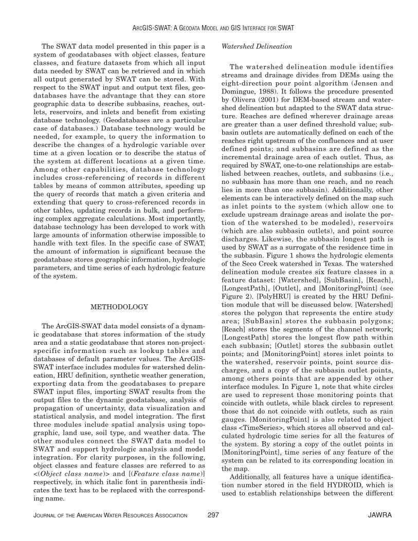
The watershed delineation module identifiesstreams and drainage divides from DEMs using theeight-direction pour point algorithm (Jensen andDomingue, 1988). It follows the procedure presentedby Olivera (2001) for DEM-based stream and water-shed delineation but adapted to the SWAT data struc-ture. Reaches are defined wherever drainage areasare greater than a user defined threshold value; sub-basin outlets are automatically defined on each of thereaches right upstream of the confluences and at userdefined points; and subbasins are defined as theincremental drainage area of each outlet. Thus, asrequired by SWAT, one-to-one relationships are estab-lished between reaches, outlets, and subbasins (i.e.,no subbasin has more than one reach, and no reachlies in more than one subbasin). Additionally, otherelements can be interactively defined on the map suchas inlet points to the system (which allow one toexclude upstream drainage areas and isolate the por-tion of the watershed to be modeled), reservoirs(which are also subbasin outlets), and point sourcedischarges. Likewise, the subbasin longest path isused by SWAT as a surrogate of the residence time inthe subbasin. Figure 1 shows the hydrologic elementsof the Seco Creek watershed in Texas. The watersheddelineation module creates six feature classes in afeature dataset: [Watershed], [SubBasin], [Reach],[LongestPath], [Outlet], and [MonitoringPoint] (seeFigure 2). [PolyHRU] is created by the HRU Defini-tion module that will be discussed below. [Watershed]stores the polygon that represents the entire studyarea; [SubBasin] stores the subbasin polygons;[Reach] stores the segments of the channel network;[LongestPath] stores the longest flow path withineach subbasin; [Outlet] stores the subbasin outletpoints; and [MonitoringPoint] stores inlet points tothe watershed, reservoir points, point source dis-charges, and a copy of the subbasin outlet points,among others points that are appended by otherinterface modules. In Figure 1, note that white circlesare used to represent those monitoring points thatcoincide with outlets, while black circles to representthose that do not coincide with outlets, such as raingauges. [MonitoringPoint] is also related to objectclass <TimeSeries>, which stores all observed and cal-culated hydrologic time series for all the features ofthe system. By storing a copy of the outlet points in[MonitoringPoint], time series of any feature of thesystem can be related to its corresponding location inthe map.

Additionally, all features have a unique identifica-tion number stored in the field HYDROID, which isused to establish relationships between the different


ARCGIS-SWAT: A GEODATA MODEL AND GIS INTERFACE FOR SWAT

classes. These relationships are represented byarrows in Figure 2. For example, the relationshipbetween [Outlet] and [Subbasin] is established bystoring the HYDROID value of the subbasin outletpoint in the OUTLET field of the subbasin polygon.Note that in <TimeSeries>, the field FEATUREIDstores the HYDROID value of the corresponding fea-ture. The feature classes also have fields related totheir geometry (i.e., AREA for polygons and LENGTHfor lines), and [Reach], in particular, has FNODE andTNODE that store the upstream and downstreampoints of each reach segment, which are used to estab-lish the stream network topology. Other attributessuch as elevation, slope, and location (i.e., longitudeand latitude) are also included.

HRU Definition

The HRU definition module identifies unique com-binations of soil and land use within each subbasin.

Soil and land use data can be provided by the user;however, tools have been included for easy use of soildata from the State Soil Geographic (STATSGO)database (USDA-NRCS, 1995) and lookup tables forconverting different land use classifications to theSWAT classification.

The STATSGO database defines map units, each ofwhich consists of one or more polygonal areas of thesame soil type. This database, whose format is differ-ent from the one defined in USDA-NRCS (1995),includes one feature class of map-unit polygons perstate, called [(State Name)], and one object class permap unit, called <(Map unit)>. Texas, for example,has 633 map units represented by 4,031 polygons, andconsequently if the study area were in Texas, a fea-ture class [Texas] with 4,031 map unit polygons and633 map unit object classes <TX001>, <TX002>, …<TX633> would be included in the static geodatabase.In these object classes, the records refer to the differ-ent soil components of the map unit, and the fieldsstore soil properties of the component and of up to 10layers of the component, as well as the percentage ofthe component in the map unit. To speed up thedatabase operations, only the feature and object class-es of the states needed are added to the static geo-database from a source set of 48 geodatabases ofSTATSGO data (i.e., one geodatabase per state of theconterminous United States). The reader is referredto USDA-NRCS (1995) for detailed STATSGO docu-mentation on soil map units, components, and layers.Similarly, land use data consist of polygonal areaswithin which a single land use is found. Land usescan be classified with any land use classification sys-tem but should be converted to the SWAT classifica-tion system for implementation with SWAT. Thus, alookup table, that the user can modify if needed, hasbeen included to define the equivalence of the Ander-son et al. (1976), National Land Cover Dataset(NLCD) (USGS, 2004a), and SWAT land use classifi-cation systems.

Regardless of the sources of the input data, one soiltype grid and one land use grid are created. Afteridentifying the grid cells that have the same soil typeand land use within each subbasin, they are groupedtogether and converted into polygons that representHRUs. Thus, in the resulting polygon feature class,called [PolyHRU], the features have a unique combi-nation of input data. As can be seen in Figure 2,[PolyHRU] polygons have a unique identificationnumber stored in field HYDROID, which is used to establish relationships with [SubBasin] and <TimeSeries>.

Additionally, ArcGIS-SWAT calculates runoff curvenumbers (USDA-SCS, 1972) and terrain slopes perHRU. Runoff curve numbers are calculated based on



Figure 1. Feature Classes Generatedby the Watershed Delineator.

the hydrologic soil group (i.e., A, B, C, or D) of theSTATSGO map unit and on the land use in the HRU.A user defined lookup table provides information ofcurve number values for each combination of hydro-logic soil group and land use code. Terrain slopes arecalculated as the average slope in the HRU polygon.

Weather Generation

SWAT has the capability of generating synthetictime series of precipitation, temperature, solar radia-tion, wind speed, and relative humidity for each sub-basin based on station weather statistics. Theweather stations and statistics can be provided by theuser, but ArcGIS-SWAT includes a point feature class



Figure 2. Attributes of and Relationships Among the Feature Classes and the Time Series Object Class.Rectangular boxes represent feature and object classes. Text on gray background indicates the classname, and text on white background indicates the class attributes. Arrows indicate relationships.

of weather stations in the static geodatabase, called[USWeather]. [USWeather] includes the location aswell as multiannual statistics of temperature, precipi-tation, solar radiation, and wind speed for each of the12 months of the year for 1,041 National ClimaticData Center (NCDC) stations (USEPA, 2004). TheArcGIS-SWAT weather generation module assignsone station in [USWeather] to each subbasin in [Sub-Basin] based on proximity to its centroid and storesthe matches in object class <SubWGn> and theweather statistics of the assigned stations in objectclass <WGn>.

Alternatively, observed weather time series at user-provided stations can be used. As in the previous case,the weather generation module assigns a station toeach subbasin based on proximity to its centroid, butnow it stores the matches in object classes <SubPcp>,<SubTmp>, <SubSlR>, <SubWnd>, and <SubHmd>and the time series in object classes <Pcp>, <Tmp>,<SlR>, <Wnd>, and <Hmd> for precipitation, temper-ature, solar radiation, wind speed, and relativehumidity, respectively. Finally, the weather timeseries are redundantly stored in <TimeSeries> (whereall input and output temporal information is consoli-dated), and all matched weather stations are append-ed to [MonitoringPoints] and related to <TimeSeries>.

Preparing SWAT Input Files

After the data are developed and stored in thedynamic geodatabase, the input files can be prepared.The preparation of the input files consists of automat-ically retrieving information from the dynamic andstatic geodatabases, entering information on-screen,and formatting it for SWAT use.

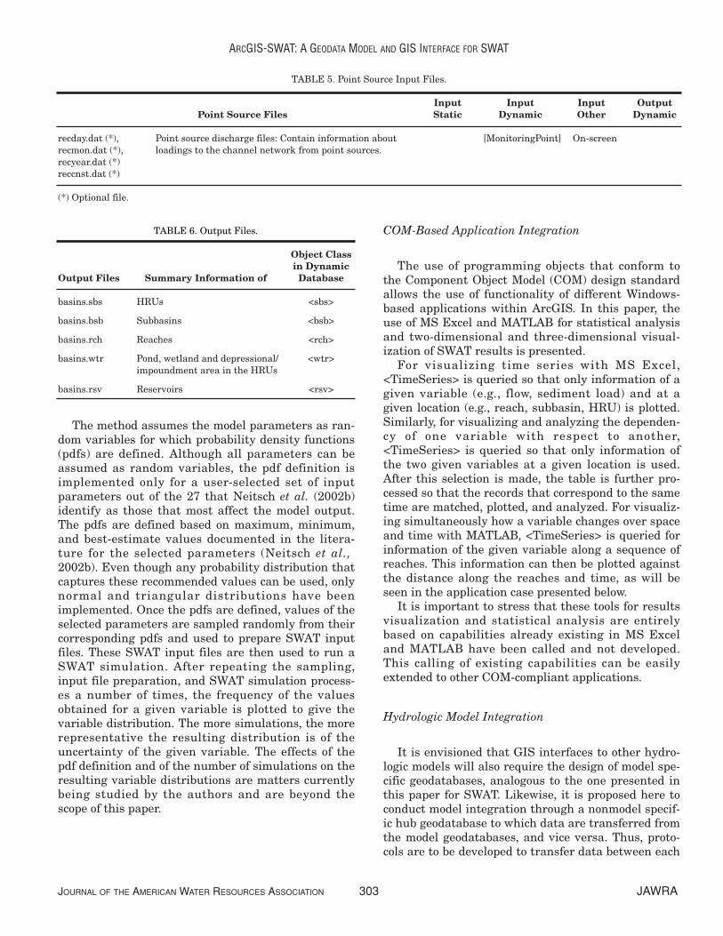
The SWAT input files can be subdivided into fivegroups: watershed files, subbasin files, HRU files,reservoir files, and point source files. Detaileddescriptions of the SWAT input files can be found inNeitsch et al. (2002b). For each group of input files,Tables 1 to 5 contain the file name in the first column;a short description of it in the second column; thesource of the data used to create the file in the third,fourth, and fifth columns; and the name of the objectclass or classes generated when creating it in the lastcolumn. The asterisk in parenthesis next to the filename indicates that its use is optional. Object classesunder the header Input/Static are not project-specificand are default SWAT values stored in the static geo-database. Object and feature classes under the headerInput/Dynamic are project specific. Note that allobject and feature classes listed under Input/Dynamicare developed by the watershed delineation, HRU def-inition, or synthetic weather generation modules and

stored in the dynamic geodatabase. The term “On-screen” under the header “Input/Other” refers toinput entered by the modeler interactively; and “Timeseries” under the same header refers to a pointer to atime series file. The object classes under the header“Output/Dynamic” are created to organize the inputentered interactively by the user. It should be notedthat user input is unavoidable in an application thatassesses the effect of human actions and land man-agement practices on water quantity and quality.

In the process of preparing the input files, soil typeand land use data are used to populate the HRU files.Soils information of the predominant STATSGO com-ponent in the HRU is transferred to the HRU soil files(HRU name).sol. Likewise, land use information isused to select, from a database of default values, HRUmanagement parameters such as the support practicefactor of the modified universal soil loss equation(Williams, 1995) or the percentage of the area wherespecific land management practices apply, such asplanting, irrigating, fertilizing, harvesting, or streetsweeping, and transfer them to the HRU manage-ment files (HRU name).mgt.

ArcGIS-SWAT also allows the user to modify thedynamic and static geodatabases and, after changesare made, create a new set of input files that reflectthese changes. Thus, the information in the geo-databases is always updated and consistent with theinput files.

Processing SWAT Output Files

After running SWAT, five output files in text for-mat are created: basins.sbs, basins.bsb, basins.rch,basins.wtr, and basins.rsv. As indicated in Table 6,each of these files contains summary information of aspecific type of hydrologic element, which is stored asan object class in the dynamic geodatabase. Addition-ally, time series data included in the five output filesare also stored in <TimeSeries>, which has fourfields: FEATURE, TYPE, TIME, and VALUE. Thesefields store where each time series record wasobserved/calculated (e.g., HRU, reach), what wasobserved/calculated (e.g., flow, sediment load), when itwas observed/calculated (e.g., day and time), and howmuch was observed/calculated (e.g., value). Thus, allof SWAT ’s output is stored in the dynamic geo-database in <sbs>, <bsb>, <rch>, <wtr> and <rsv>and in <TimeSeries>.



Propagation of Uncertainty

Uncertainty in a model’s output can be caused,among other sources, by uncertainty in the value ofthe model parameters. SWAT is a model that includesa large number of parameters. Each of the parame-

ters is known with a different level of accuracy andtakes part in a different hydrologic process. Assessingthis uncertainty in an analytical way is not alwayspossible. The authors have developed a method basedon Monte Carlo simulations that generates frequencydistributions of the SWAT output variables (asopposed to a single value).



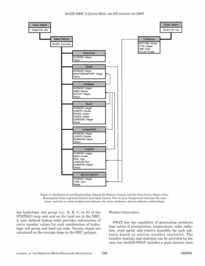
TABLE 1. Watershed Input Files.

Input Input Input OutputWatershed Files Static Dynamic Other Dynamic

file.cio Control input/output file: Contains names of input [Watershed], On screenfiles for all watershed and subbasin level variables. <SubWGn>,

<SubPcp> (*),<SubTmp> (*),<SubSlR> (*),<SubWnd> (*),<SubHmd> (*)

basins.fig Watershed configuration file: Defines the routing [Reach],network in the watershed. [MonitoringPoint]

basins.cod Input control code file: Specifies the length of the On screen <cod>simulation, the printing frequency and selectedoptions for various processes.

basins.bsn Basin input file: Stores watershed parameters [Watershed] On screen <bsn>

pcp.pcp (*) Precipitation file: Stores daily measured precipitation <Pcp> (*)for a number of gauges.

tmp.tmp (*) Temperature file: Stores daily measured maximum <Tmp> (*)and minimum temperature for a number of gauges.

slr.slr (*) Solar radiation file: Stores daily solar radiation for <SlR> (*)a number of gauges.

wnd.wnd (*) Wind file: Stores daily average wind speed for a <Wnd> (*)number of gauges.

hmd.hmd (*) Humidity file: Stores daily relative humidity for a <Hmd> (*)number of gauges.

pet.pet (*) Potential evapotranspiration file: Stores daily potential Time series (*)evapotranspiration for the watershed.

crop.dat Land cover and plant growth file: Contains plant <Crop>growth parameters for all land covers in the watershed.

fert.dat Fertilizer file: Contains information on the nutrient <Fert>content for all fertilizers and manures in the watershed.

pest.dat Pesticide file: Contains information on mobility and <Pest>degradation for all pesticides in the watershed.

till.dat Tillage file: Contains information on the amount and <Till>depth of mixing caused by tillage operations in thewatershed.

urban.dat Urban file: Contains information on the build-up/ <Urban>wash-off of solids in urban areas in the watershed.

basins.wwq (*) Water quality file: Contains QUAL2E parameters to On screenmodel transformations in the main channels.

(*) Optional file.



TABLE 2. Subbasin Input Files.

Input Input Input OutputSubbasin Files Static Dynamic Other Dynamic

(Subbasin name).sub Subbasin file: Stores subbasin parameters – [SubBasin], <sub>[LongestPath],[PolyHRU]

(Subbasin name).pnd (*) Pond/wetland file: Contains information for impound- – [SubBasin] On screen <Pnd>ments within the subbasin.

(Subbasin name).wus (*) Water use file: Contains information for consumptive – [SubBasin] On screen <WUs>water use in the subbasin.

(Subbasin name).rte Main channel file: Contains parameters governing water – [SubBasin] On screen <RTE>and sediment movement in the main channel of thesubbasin.

(Subbasin name).swq (*) Stream water quality file: Contains parameters to model – [SubBasin] On screen <SQW>pesticide and QUAL2E nutrient transformations in themain channel of the subbasin.

(Subbasin name).wgn Weather generator file: Contains statistical data – [SubBasin]needed to generate synthetic daily climatic data for the <WGn>subbasins. [MonitoringPoint]

(*) Optional file.

TABLE 3. HRU Input Files.

Input Input Input OutputHRU Files Static Dynamic Other Dynamic

(HRU name).hru HRU file: HRU parameters – [PolyHRU] On screen <HRU>

(HRU name).sol Soil file: Contains information about the physical – [PolyHRU], On screen <Sol>properties of the soils in the HRU. <(Map Unit)>

(HRU name).chm (*) Soil chemical file: Contains information about the initial – [PolyHRU] On screen <Chm>nutrient and pesticide levels of the soil in the HRU.

(HRU name).gw Ground water file: Contains information about the – [PolyHRU] On screen <GW>shallow and deep aquifer in the subbasin.

(HRU name).mgt Land management file: Contains management scenarios <Irr> [PolyHRU] On screen <Mgt1>,and specifies the land cover in the HRU. <MgtType>, <Mgt2>

<MgtDate>,<MgtSCS>

(*) Optional file.

TABLE 4. Reservoir Input Files.

Input Input Input OutputReservoir Files Static Dynamic Other Dynamic

basins.res (*) Reservoir file: Contains parameters to model the movement – [SubBasin] On screen <Res>of water and sediment through a reservoir.

basins.lwq (*) Lake water quality file: Contains parameters to model the – [SubBasin] On screen <Res>movement of nutrients and pesticides through a reservoir.

(*) Optional file.

The method assumes the model parameters as ran-dom variables for which probability density functions(pdfs) are defined. Although all parameters can beassumed as random variables, the pdf definition isimplemented only for a user-selected set of inputparameters out of the 27 that Neitsch et al. (2002b)identify as those that most affect the model output.The pdfs are defined based on maximum, minimum,and best-estimate values documented in the litera-ture for the selected parameters (Neitsch et al.,2002b). Even though any probability distribution thatcaptures these recommended values can be used, onlynormal and triangular distributions have beenimplemented. Once the pdfs are defined, values of theselected parameters are sampled randomly from theircorresponding pdfs and used to prepare SWAT inputfiles. These SWAT input files are then used to run aSWAT simulation. After repeating the sampling,input file preparation, and SWAT simulation process-es a number of times, the frequency of the valuesobtained for a given variable is plotted to give thevariable distribution. The more simulations, the morerepresentative the resulting distribution is of theuncertainty of the given variable. The effects of thepdf definition and of the number of simulations on theresulting variable distributions are matters currentlybeing studied by the authors and are beyond thescope of this paper.

COM-Based Application Integration

The use of programming objects that conform tothe Component Object Model (COM) design standardallows the use of functionality of different Windows-based applications within ArcGIS. In this paper, theuse of MS Excel and MATLAB for statistical analysisand two-dimensional and three-dimensional visual-ization of SWAT results is presented.

For visualizing time series with MS Excel, <TimeSeries> is queried so that only information of agiven variable (e.g., flow, sediment load) and at agiven location (e.g., reach, subbasin, HRU) is plotted.Similarly, for visualizing and analyzing the dependen-cy of one variable with respect to another, <TimeSeries> is queried so that only information ofthe two given variables at a given location is used.After this selection is made, the table is further pro-cessed so that the records that correspond to the sametime are matched, plotted, and analyzed. For visualiz-ing simultaneously how a variable changes over spaceand time with MATLAB, <TimeSeries> is queried forinformation of the given variable along a sequence ofreaches. This information can then be plotted againstthe distance along the reaches and time, as will beseen in the application case presented below.

It is important to stress that these tools for resultsvisualization and statistical analysis are entirelybased on capabilities already existing in MS Exceland MATLAB have been called and not developed.This calling of existing capabilities can be easilyextended to other COM-compliant applications.

Hydrologic Model Integration

It is envisioned that GIS interfaces to other hydro-logic models will also require the design of model spe-cific geodatabases, analogous to the one presented inthis paper for SWAT. Likewise, it is proposed here toconduct model integration through a nonmodel specif-ic hub geodatabase to which data are transferred fromthe model geodatabases, and vice versa. Thus, proto-cols are to be developed to transfer data between each



TABLE 5. Point Source Input Files.

Input Input Input OutputPoint Source Files Static Dynamic Other Dynamic

recday.dat (*), Point source discharge files: Contain information about [MonitoringPoint] On-screenrecmon.dat (*), loadings to the channel network from point sources.recyear.dat (*) reccnst.dat (*)

(*) Optional file.

TABLE 6. Output Files.

Object Classin Dynamic

Output Files Summary Information of Database

basins.sbs HRUs <sbs>

basins.bsb Subbasins <bsb>

basins.rch Reaches <rch>

basins.wtr Pond, wetland and depressional/ <wtr>impoundment area in the HRUs

basins.rsv Reservoirs <rsv>

model geodatabase and the hub geodatabase, inde-pendently of other models. According to thisapproach, the number of required protocols wouldincrease linearly with the number of models, becauseone protocol would be needed per model. On the con-trary, if no hub geodatabase were used and data weretransferred between each match of two model geo-databases, the number of protocols would be equal tothe combination of the number of models taken two ata time, which is equal to where n is the number ofmodels. The hub geodatabase can be as simple or com-plex as needed, depending on the models that will beintegrated and on the data that will be shared. Thehub-geodatabase concept stems from Olivera et al.(2003), in which ArcHydro (Maidment, 2002) was pro-posed as the hub geodatabase. However, the pointconveyed here is that any geodatabase that can storethe hydrologic elements common to the models thatare being integrated (including ArcHydro) can be usedas the hub geodatabase.

The hub geodatabase presented here addresses thehydrologic elements and their topologic relationshipsand is suitable for integrating models that share thesame watershed structure and stream network. Itincludes five feature classes: [Stream], [ExitPoint],[DrainageArea], [Lake], and [Station]. [Stream] storesthe segments of the channel network; [ExitPoint]stores the points on the channel network from whichdrainage areas are delineated; [DrainageArea] storesthe incremental drainage area of each point in [Exit-Point]; [Lake] stores outlet points of water bodies onthe channel network from which drainage areas aredelineated; and [Station] stores the points where pre-cipitation, flow gauging, and/or water quality moni-toring stations are located. All features in the fivefeature classes have a unique identification numberstored in a field called ID. Additionally, the featuresare cross referenced through the ID field so thatdrainage areas are related to their exit points,streams are related to the drainage area where theyare located, and lakes are related to the exit pointthat represents them. Likewise, [Stream] includesfields FNODE and TNODE that store identificationcodes of the upstream and downstream nodes of thesegments, which are used for establishing the net-work topology.

Once the hub geodatabase is populated – for exam-ple, by copying features and attributes from theSWAT geodatabases – its contents can be used byanother model interface. As an application example,the use of data developed by ArcGIS-SWAT andstored in the hub geodatabase for creating an HEC-HMS model is demonstrated. The tool to retrieve thedata from the hub geodatabase and format it forHEC-HMS is a separate application and is not part of

ArcGIS-SWAT. It has been presented here only tostress the advantages of the use of the geodatabaseand hub geodatabase approach.

APPLICATION

ArcGIS-SWAT was applied to the Upper SecoCreek in Central Texas for which studies have beenconducted in the past (Srinivasan and Arnold, 1994;Baird et al., 1996; Brown and Raines, 2002) and dataare available. The Upper Seco Creek is part of theNueces basin (Figure 3). The study area was thecatchment of U.S. Geological Survey (USGS) gaugingstation 08201500 (Seco Creek at Miller Ranch nearUtopia), which has a drainage area of 116 km2.

Daily precipitation data were obtained from twostations set as part of the Seco Creek Water QualityDemonstration Project (Brown et al., 1998; Brown andRaines, 2002) (Figure 3). Likewise, daily flow datawere obtained for USGS flow gauging station08201500 (USGS, 2006) (Figure 3). Temperature,solar radiation, wind, and humidity data were gener-ated from the weather statistics stored in [USWeath-er]. Topographic data in DEM format, with ahorizontal resolution of 10 m, were obtained fromUSGS (2004b). Streams were delineated for drainageareas greater than 2 km2 (i.e., 20,000 DEM cells), anda total of 39 stream-subbasin-outlet sets were identi-fied (Figure 1). Land use data in grid format, with ahorizontal resolution of 30 m, were taken from NLCD



Figure 3. The Seco Creek Watershed is Part of the NuecesRiver Basin (in gray) in Texas. Points 2941250992554 and

2937170992513 are the rain gauges located at 99°25´54´´W,29°41´25´Ń and 99°25´13´´W, 29°37´17´Ń; and pointUSGS08201500 is the flow gauging station located at99°24´10´´W, 29°34´23´Ń. The stream highlighted in

black is the longest flow path in the watershed.

(USGS, 2004a) (Figure 4a). Soil data were retrievedfrom the STATSGO database (USDA-NRCS, 1995) included in the static geodatabase. The STATSGOmap units in the watershed were TX155 and TX525,which covered 81 percent and 19 percent of its area,respectively (Figure 4b). In both map units, the hydro-logic soil group of the dominant soil component was D.A curve number grid, with the same resolution as theDEM, was generated based on the land use and soilsdata. Unique combinations of subbasins, land use,and soil type led to a total of 323 HRUs in the water-shed (Figure 5).

SWAT input files were prepared based on thehydrologic features and parameters developed andstored in the dynamic geodatabase. The model config-uration considered: curve number method for runoffdepth calculation; daily time step (which follows fromthe use of the curve number method); Priestley-Taylormethod for potential evapotranspiration calculation;and Muskingum method for stream routing. The read-er is referred to the SWAT theoretical documentation(Neitsch et al., 2002a) for further discussion on theseoptions.

The simulation period ran from January 1991 toJune 1994. January 1991 to December 1992 was usedfor calibrating the model, and January 1993 to June1994 was used for validating it. Given that SWATrequires an initial stabilization period, the model wasrun for three years before the actual simulation peri-od started. The stabilization period is necessarybecause during the first years of simulation, themodel output is affected by the estimated (and notcalculated) initial conditions, such as soil water con-tent and surface residue. Although there is no rule todetermine the duration of the stabilization period,three years was used in accordance to Santhi et al.’s(2001) work in the North Bosque River watershed inTexas. The model was calibrated for daily flows fol-lowing the steps recommended by Neitsch et al.(2002b). Observed and simulated monthly flows arepresented in Figure 6. After running the model, allinput data and simulation results, including geo-graphic information, hydrologic parameters, and timeseries, were stored in the dynamic geodatabase. Thegoodness of fit of the hydrographs was quantified withthe deviation of runoff volumes Dv (Martinec andRango, 1989) and the Nash-Sutcliffe efficiency coeffi-cient ENS (Nash and Sutcliffe, 1970). Note that a per-fect model produces a value of Dv of zero, and of ENSof one. The reader is referred to the American Societyof Civil Engineers (1993) for a detailed discussion oncriteria for evaluation of watershed models.



Figure 4. Seco Creek Watershed: (a) Land Use/cover Accordingto NLCD: Forest (white), Urban (black), and Agriculture,

Pasture and Others (gray); (b) Soils According to theSTATSGO Database: TX155 (gray) and TX525 (white).

Figure 5. Hydrologic Response Units of the Seco Creek Watershed.Note that an HRU can be a complex polygon, that is, an

object consisting of a series of disconnected polygons,like those shown in black in the insert.

For the calibration period, it was found that Dv wasequal to 0.01 for 1991 and 0.11 for 1992; for the vali-dation period, Dv was equal to -0.04 for 1993. Basedon daily flows, it was found that ENS was equal to0.67 for the calibration period and 0.33 for the valida-tion period. Similarly, based on monthly flows, it wasfound that ENS was equal to 0.88 and 0.90 for the cal-ibration and validation periods, respectively. Compa-rable values of Dv and ENS for daily and monthlyflows simulated with SWAT are found in the litera-ture (Hanratty and Stefan, 1998; King et al., 1999;Rosenthal and Hoffman 1999; Spruill et al., 2000;Eckhardt and Arnold, 2001; Weber et al., 2001;Fontaine et al., 2002; Neitsch et al., 2002c; Eckhardtet al., 2003; Tripathi et al., 2003). The value of ENS of0.33 for the validation period with daily flows, though,is lower than what was found in the literature. Possi-ble causes of this discrepancy include the fact that themodel was calibrated for a period in which flows weresignificantly higher than those in the validation peri-od and that the values of some of the weather vari-ables were generated and not measured. Likewise,undistinguishable simulated flows were observedwhen the terrain parameters were calculated perHRU or averaged per subbasin. It is likely that this iscaused by the fact that the analysis time step is muchlarger than the subbasins’ time of concentration. Itwould be expected that the effect of estimating thehydrologic parameters per HRU would make a differ-ence in simulations with longer times of concentrationand/or shorter time steps.

Additionally, the lack of observed constituent loadtime series did not allow for proper calibration of themodel for water quality. Still, model parameters wereestimated using Baird et al.’s (1996) median sedimentconcentration of 245 mg/l, which was calculated from81 discrete samples collected from 1970 to 1995 atstation 08201500. Two of these calculated parameters

were α and β in the channel sediment transport equa-tion (Neitsch et al., 2002b)

c = α vβpeak

where c (kg/l) is the maximum concentration of sedi-ment that can be transported by the flow and v (m/s)is the peak channel velocity. It was found that α =0.001 and β = 1.5. Since the calculation of theseparameters considered only Bairds et al.’s (1996) esti-mated median concentration, to account for the uncer-tainty in the sediment loads caused by theuncertainty in these two parameters, 1,000 SWATsimulations were run for different combinations ofvalues of α and β. The values of α were drawn ran-domly from a triangular pdf of log α, in which theminimum and maximum values of α were 0.0001 and0.01, as recommended by Neitsch et al. (2002b), andthe mode 0.001 (i.e., the value of α obtained previous-ly). Similarly, the value of β was drawn randomlyfrom a triangular pdf, in which the minimum andmaximum values were 1 and 2, as recommended byNeitsch et al. (2002b), and the mode 1.5 (i.e., the valueof β obtained previously). The resulting cumulativefrequency distribution of the 3.5-year median sedi-ment concentration at Station 08201500 is shown inFigure 7. From the figure, it can be concluded, forexample, that there is a 33 percent chance of obtain-ing a median concentration greater than 400 mg/l, ora 10 percent chance of obtaining a median concentra-tion greater than 900 mg/l. The minimum number ofsimulations necessary to realistically capture the dis-tribution of a variable is currently a matter ofresearch by the authors. The number of 1,000 waschosen because it was observed that the mean andstandard deviation of the distribution were not affect-ed by additional simulations.



Figure 6. Observed and Simulated Monthly Flows atUSGS Flow Gauging Station 08201500 (USGS, 2006).

(1)

Figure 7. Probability That the Median SedimentConcentration Will Exceed a Given Value.

Likewise, the tools for visualization and statisticalanalysis of the SWAT output called MS Excel COMobjects and used their functionality within ArcGIS forplotting the time series of monthly sediment load(Figure 8a) and monthly sediment load as a functionof the monthly flow (Figure 8b) and performing statis-tical analysis (i.e., trend line). Correlation and regres-sion analysis, as well as analysis of variance (ANOVA)can also be performed by MS Excel but are not dis-cussed here. In these plots, it was observed that thesediment load was concentrated in a few number ofmonths and that it was correlated to the monthly flowwith an r2 of 0.92. Similarly, the tools called MATLABCOM objects and used their functionality for develop-ing a three-dimensional plot of the flow profile of thelongest flow path in the watershed (Figure 8c) (thelongest flow path has been highlighted in black inFigure 3). This three-dimensional plot allows one toobserve the flow at a given point over time and theflow at a given time over the entire stream. Variablesother than flow and sediment load can also be plottedand analyzed.

Finally, the streams and watersheds delineated byArcGIS-SWAT and stored in the dynamic geodatabasewere copied to the hub geodatabase, from whichanother application (unrelated to ArcGIS-SWAT)retrieved them and created a topologically correctschematic of the watershed for hydrologic analysiswith HEC-HMS (Figure 9). Thus, it is demonstratedthat a hub geodatabase can be used to share geo-graphic data between different applications and thatthe use of data developed by ArcGIS-SWAT is not lim-ited to SWAT.

CONCLUSIONS

ArcGIS-SWAT consists of a data model and a GISinterface (i.e., pre-processor and post-processor) forSWAT. With respect to previous data models and GISinterfaces for SWAT, the ArcGIS-SWAT data modeluses the geodatabase structure, which can store geo-graphic as well as numeric and text information, andthe interface uses programming objects that conformto the COM protocol, thus allowing the use of func-tionality of other COM compliant applications (i.e.,Windows-based applications). ArcGIS-SWAT extractshydrologic information from spatial data (delineatesstreams and watersheds, defines HRUs and assignsparameter values based on their soil type and landuse, and matches subbasins and weather stationsbased on location), stores it in the data model, uses itfor preparing SWAT input files, runs SWAT, andwrites the SWAT output on the data model. Because

of the geodatabase capability to store geographicinformation, it constitutes a complete repository of asimulation’s data and results, something not possiblewith the SWAT text input and output files.



Figure 8. Output Visualization Tools: (a) Time Series of SedimentLoad at the Watershed Outlet, (b) Sediment Load Versus Flow

at the Watershed Outlet, and (c) Flow Versus Time andDistance for the Watershed’s Longest Flow Path.

(c)

(b)

(a)

A feature of ArcGIS-SWAT is its capability to geo-reference the HRUs, which allows accounting for theHRU’s location within the subbasin and the estima-tion of individual parameter values, without lumpingthem over their subbasin. However, the quantificationof the effect of accounting for the HRU’s location onflows and loads was beyond the scope of this paper.The use of Monte Carlo simulations in combinationwith the ArcGIS-SWAT data model allows the estima-tion of the uncertainty of the SWAT results by produc-ing frequency distributions of the variables ratherthan a single value. By generating results such as“there is a 10 percent chance that the median sedi-ment concentration will be greater than 900 mg/l,” themodeler is provided valuable information for inter-preting the SWAT output. Likewise, the use of pro-gramming objects that conform the COM protocolallowed the implementation of functionality of otherWindows-based applications within ArcGIS. In partic-ular, the use of MS Excel functionality for plottingand regression analysis as well as of MATLAB func-tionality for three-dimensional plotting was demon-strated. For model integration, the use of a hubgeodatabase that stores geographic and hydrologicdata relevant to different models is proposed anddemonstrated. In particular, it was presented howinformation developed by ArcGIS-SWAT for use bySWAT was transferred to the hub geodatabase, fromwhich it was retrieved by another application andused to create an HMS model for flood analysis. It isenvisioned that the use of the hub geodatabase con-cept will ease model integration.

With respect to previous SWAT GIS interfaces,ArcGIS-SWAT takes advantage of programming tech-nology – such as the geodatabase data structure and

COM objects – for exchange of computer applicationfunctionality and hydrologic model integration. How-ever, it is considered that hydrologic model integra-tion is more a long term goal than a short term taskand that the geodatabase and hub geodatabaseapproach presented in this paper is a step in thisdirection but at the same time, that further workalong these lines, including the implementation witha wide variety of models, is necessary to assess theadvantages of this new concept and the needs for thegeodatabase structures.

ACKNOWLEDGMENTS

The authors would like to thank three anonymous manuscriptreviewers whose input has been fundamental for improving thetext. This work has been conducted with support of the U.S. ArmyCorps of Engineers-Fort Worth District in Texas.

LITERATURE CITED

American Society of Civil Engineers, 1993. Criteria for Evaluationof Watershed Models. ASCE Task Committee on the Definitionof Criteria for Evaluation of Watershed Models of the WatershedManagement Committee, Irrigation and Drainage Committee.Journal of Irrigation and Drainage Engineering 119(3):429-442.

Anderson, J.R., E.E. Hardy, J.T. Roach, and R.E. Witmer, 1976. ALand Use and Land Cover Classification System for Use WithRemote Sensor Data. Geological Survey Professional Paper 964,U.S. Government Printing Office, Washington D.C. Available athttp://landcover.usgs.gov/pdf/anderson.pdf. Accessed on April 21,2004.

Arnold, J.G., R. Srinivasan, R.S. Muttiah, and J.R. Williams, 1998.Large Area Hydrologic Modeling and Assessment – Part I:Model Development. Journal of the American Water ResourcesAssociation (JAWRA) 34(1):73-89.

Baird, C., M. Jennings, D. Ockerman, and T. Dybala, 1996. Charac-terization of Nonpoint Sources and Loadings to the CorpusChristi Bay National Estuary Program Study Area. CorpusChristi Bay National Estuary Program CCBNEP–05, 226 pp.,Texas Natural Resources Conservation Commission (TNRCC),Austin, Texas.

Bian, L., H. Sun, C. Blodgett, S. Egbert, L. WeiPing, R. LiMei, andA. Koussis, 1996. An Integrated Interface System to Couple theSWAT Model and ARC/INFO. In: Proceedings of the 3rd Inter-national Conference on Integrating GIS and EnvironmentalModeling. U.S. National Center for Geographic Information andAnalysis, Santa Fe, New Mexico, CD-ROM.

Brown, D. and T. Raines, 2002. Simulation of Flow and Effects ofBest Management Practices in the Upper Seco Creek Basin,South-Central Texas, 1991-98. U.S. Geological Survey WaterResources Investigations Report 02-4249, Austin, Texas.

Brown, D., R. Slattery, and J. Gilhousen, 1998. Summary Statisticsand Graphical Comparisons of Historical Hydrologic and Water-Quality Data, Seco Creek Watershed, South-Central Texas. U.S.Geological Survey Open-File Report 98-627, 37 pp.

Di Luzio, M., R. Srinivasan, and J.G. Arnold, 1998. Watershed Ori-ented Non-point Pollution Assessment Tool. In: Proceedings ofthe 7th International Conference on Computers in Agriculture.American Society of Agricultural Engineers, St. Joseph, Michi-gan, pp. 233-241.



Figure 9. HMS Model of the Seco Creek Watershed.

Di Luzio, M., R. Srinivasan, and J.G. Arnold, 2002. Integration ofWatershed Tools and SWAT Model Into BASINS. Journal of theAmerican Water Resources Association (JAWRA) 38(4):1127-1141.

Di Luzio, M., R. Srinivasan, J.G. Arnold, and S.L. Neitsch, 2000.Soil and Water Assessment Tool – ArcView GIS Interface Manu-al – Version 2000. Grassland, Soil and Water Research Labora-tory, Agricultural Research Service and Blackland ResearchCenter, Texas Agricultural Experiment Station, Temple, Texas.

Eckhardt, K. and J.G. Arnold, 2001. Automatic Calibration of a Dis-tributed Catchment Model. Journal of Hydrology 251(2001):103-109.

Eckhardt, K., L. Breuer, and H.G. Frede, 2003. Parameter Uncer-tainty and the Significance of Simulated Land Use ChangeEffects. Journal of Hydrology 273(2003):164-176.

Fontaine, T.A., T.S. Cruickshank, J.G. Arnold, and R.H. Hotchkiss,2002. Development of a Snowfall-Snowmelt Routine for Moun-tainous Terrain for SWAT. Journal of Hydrology 262(2002):209-223.

Hanratty, M.P. and H.G. Stefan, 1998. Simulating Climate ChangeEffects in a Minnesota Agricultural Watershed. Journal of Envi-ronmental Quality 27:1524-1532.

Jensen, S.K. and J.O. Domingue, 1988. Extracting TopographicStructure From Digital Elevation Data for Geographic Informa-tion System Analysis. Photogrammetric Engineering andRemote Sensing 54(11).

King, K.W., J.G. Arnold, and R.L. Bingner, 1999. Comparison ofGreen-Ampt and Curve Number Methods on Goodwin CreekWatershed Using SWAT. Transactions ASAE 42(4):919-925.

MacDonald, A., 1999. Building a Geodatabase. ESRI Press, Red-lands, California.

Maidment, D.R. (Editor), 2002. ArcHydro: GIS for Water Resources.ESRI Press, Redlands, California.

Martinec, J. and A. Rango, 1989. Merits of Statistical Criteria forthe Performance of Hydrological Models. Water Resources Bul-letin 25(2):421-432.

Nash, J.E. and J.E. Sutcliffe, 1970. River Flow Forecasting ThroughConceptual Models – Part 1-A: Discussion of Principles. Journalof Hydrology 10(82):282-290.

Neitsch, S.L., J.G. Arnold, J.R. Kiniry, J.R. Williams, and K.W.King, 2002a. Soil and Water Assessment Tool – Theoretical Doc-umentation – Version 2000. Grassland, Soil and Water ResearchLaboratory, Agricultural Research Service and BlacklandResearch Center, Texas Agricultural Experiment Station, Tem-ple, Texas.

Neitsch, S.L., J.G. Arnold, J.R. Kiniry, R. Srinivasan, and J.R.Williams, 2002b. Soil and Water Assessment Tool – User’s Man-ual – Version 2000. Grassland, Soil and Water Research Labora-tory, Agricultural Research Service and Blackland ResearchCenter, Texas Agricultural Experiment Station, Temple, Texas.

Neitsch, S.L., J.G. Arnold, and R. Srinivasan, 2002c. Pesticides Fateand Transport Predicted by the Soil and Water Assessment Tool(SWAT) – Atrazine, Metolachlor and Trifluralin in the Sugar Creek Watershed. Grassland, Soil and Water Research Labora-tory, Agricultural Research Service and Blackland ResearchCenter, Texas Agricultural Experiment Station, Temple, Texas.

Olivera, F., 2001. Extracting Hydrologic Information From SpatialData for HMS Modeling. Journal of Hydrologic Engineering 6(6):524-530.

Olivera, F., R. Dodson, and D. Djokic, 2003. Use of Arc Hydro forIntegration of Hydrologic Applications. In: Proceedings of theAmerican Society of Civil Engineers (ASCE) World Water andEnvironmental Resources Congress 2003, Philadelphia, Penn-sylvania. American Society of Civil Engineers (ASCE), Reston,Virginia, doi 10.1061/40685(2003)249.

Olivera, F., D.R. Maidment, and D. Honeycutt, 2002. HydroNet-works. In: ArcHydro: GIS for Water Resources, D.R. Maidment(Editor). ESRI Press, Redlands, California, pp. 33-53.

Rosenthal, W.D. and D.W. Hoffman, 1999. Hydrologic Modeling/GISas an Aid in Locating Monitoring Sites. Transactions ASAE 42(6):1591-1598.

Santhi, C., J.G. Arnold, J.R. Williams, W.A. Dugas, R. Srinivasan,and L.M. Hauck, 2001. Validation of the SWAT Model on aLarge River Basin With Point and Nonpoint Sources. Journal ofAmerican Water Resources Association (JAWRA) 37(5):1169-1188.

Spruill, C.A., S.R. Workman, and J.L. Taraba, 2000. Simulation ofDaily and Monthly Stream Discharge From Small WatershedsUsing the SWAT Model. Transactions ASAE 43(6):1431-1439.

Srinivasan, R. and J.G. Arnold, 1994. Integration of a Basin-ScaleWater Quality Model With GIS. Journal of the American WaterResources Association (JAWRA) 30(3):453-462.

Tripathi, M.P., R.K. Panda, and N.S. Raghuwanshi, 2003. Identifi-cation and Prioritization of Critical Sub-Watersheds for SoilConservation Management Using the SWAT Model. BiosystemsEngineering 85 (3):365-379.

USACE (U.S. Army Corps of Engineers), 2005. Hydrologic ModelingSystem – HEC-HMS – User’s Manual, Vol. 3.0.0. U.S. ArmyCorps of Engineers-Hydrologic Engineering Center, CPD-74A,Davis, California.

USDA-NRCS (U.S. Department of Agriculture-Natural ResourcesConservation Service), 1995. State Soil Geographic (STATSGO)Database – Data User Guide. U.S. Department of Agriculture,Natural Resources Conservation Service, Miscellaneous Publica-tion Number 1492, Washington D.C.

USDA-SCS (U.S. Department of Agriculture-Soil Conservation Ser-vice), 1972. National Engineering Handbook – Section 4:Hydrology. U.S. Department of Agriculture, Soil ConservationService, Washington, D.C.

USEPA (U.S. Environmental Protection Agency), 2004. BASINS:Better Assessment Science Integrating Point and NonpointSources – NOAA’s National Climatic Data Centers (NCDC)Weather Data Management (WDM) Stations Point Locations inthe United States, Puerto Rico, and the U.S. Virgin Islands.Available at http://www.epa.gov/waterscience/basins/metadata/wdm.htm. Accessed on September 30, 2004.

USGS (U.S. Geological Survey), 2004a. National Land CoverDataset 1992 (NLCD 1992). Available at http://landcover.usgs.gov/natllandcover.asp. Accessed on April 2004.

USGS (U.S. Geological Survey), 2004b. Seamless Data DistributionSystem, Earth Resources Observation and Science (EROS).Available at http://seamless.usgs.gov/. Accessed on April 2004.

USGS (U.S. Geological Survey), 2006. Daily Streamflow for theNation. Available at http://nwis.waterdata.usgs.gov/usa/nwis/discharge. Accessed in January 2006.

Weber, A., N. Fohrer, and D. Moller, 2001. Long-Term Land UseChanges in a Mesoscale Watershed Due to Socio-Economics Fac-tors – Effects on Landscape Structures and Functions. Ecologi-cal Modeling 140:125-140.

Williams, J.R., 1995. The EPIC Model. In: Computer Models ofWatershed Hydrology, V.P. Singh (Editor). Water Resources Pub-lications, Highlands Ranch, Colorado, pp. 909-1000.

Zeiler, M., 2001. Exploring ArcObjects. ESRI Press, Redlands, Cali-fornia.



arcgis-swat: a geodata model and gis interface …ceprofs.tamu.edu/folivera/papers pdfs/2006 arcgis...

Documents