1

Molecular Dynamics Calculations using NAMD

Dr Karina Kubiak – Ossowska High Performance Computing Support

Team Department of Physics

e-mail: karina.kubiak@strath.ac.uk

A. Introduction NAMD (Fig.1), is a parallel molecular dynamics code designed for high-performance simulations of large biomolecular systems. Based on Charm++ parallel objects NAMD scales to hundreds of thousands of processors on high-end parallel platforms and tens of processors on commodity clusters using gigabit ethernet. NAMD uses the popular molecular graphics program VMD for simulation setup and trajectory analysis, but is also file-compatible with AMBER, CHARMM, and X-PLOR. NAMD is distributed free of charge with source code. Detailed description of NAMD may be found at http://www.ks.uiuc.edu/Research/namd/. The detailed guide and tutorial for NAMD may be downloaded from http://www.ks.uiuc.edu/Research/namd/2.7/ug/ and http://www.ks.uiuc.edu/Training/Tutorials/namd/namd-tutorial-win.pdf, respectively. The instructions below do not explain every detail, but it provides a simple guide on how to run basic simulations (protein in water box) instead.

2

Fig. 1. NAMD Web page

B. Standard simulations Check the computer system to ensure all programs are installed. If you are working on ARCHIE-WeSt all example files can be found at the directory: /users/cwb08102/NAMD_Training

Check what modules are loaded by typing: module list

check what modules are available to load by typing: module avail

load the modules by typing: module load /apps/bin/vmd/1.9.1 module load /mpi/gcc/openmpi/1.4.5 module load /libs/gcc/fftw2/float-mpi/2.1.5 module load /apps/gcc/namd/mpi/2.8

Note: The way you set up your account and environment depends on computer system you work on.

1. Protein structure

3

To simulate the protein first we need the x,y,z coordinates of each atom in the protein. Such information is deposited in the PDB (protein data bank) which consist of X-ray as well as NMR protein structures. Due to technical reasons, X-ray structures are available for large proteins only. The main difference between NMR and X-ray structures is that in NMR structures hydrogen atoms are included while there are no hydrogen atoms in X-ray structure (H atoms are too light to X-ray diffraction experiments). Usually we are interested in large proteins and that is why calculations using the X-ray structure as a first example are described.

a) Download the correct structure Go to PDB (http://www.rcsb.org/pdb/home/home.do), and look for protein structure you are interested in (Fig.2). Let’s say that you are looking for hen egg white lysozyme (HEWL). If you already know the PDB ID (1iee) you can type it in the first text window. Usually you don’t know the ID, so give the protein name (e.g. hen egg white lysozyme) in the second text window and click search. You will see a lot of records. There is more than one structure deposited in PDB, so look for the protein obtained with the highest resolution, without ligands and protein engineering procedures. We need the native structure. Check the year when the structure was published, read carefully records provided about structure details and download the original paper describing the structure published (Fig. 3). Once you are sure it is the right structure, download it to your computer in the pdb format (Fig. 3). Let’s call this file protein_original.pdb.

Fig.2. Protein Data Bank (pdb) starting page

4

Fig. 3. PDB – searching result and Download the structure

b) See the protein Open the vmd program and then go to Main menu → File → New molecule →

protein_original.pdb. The other way to see the protein is type in your terminal command line vmd protein_original.pdb, the result will be exactly the same. Now play in VMD: rotate the protein, change the representation (Main menu → Graphics → Representations), and view the protein structure. Read the VMD tutorial to learn how to visualize and present the protein, how to change colors, how to highlight only a chosen residue etc.

2. Prepare the simulations The *.psf file together with *.pdb contain all information about our protein. The *.pdb file includes only initial coordinates of atoms, the *.psf file includes all other information (bond length, angles, force constants, charges, van der Waals parameters etc.). The psf file is created basing on the *.pdb file and the top_all27_prot_na.inp (the topology file). Since it is possible to change the topology file by adding new parameters it is better to use the file top_all27_prot_surf.inp created by myself.

a) Prepare the pdb file Open the protein_original.pdb file using vi or any other editor. Read the file, check if there are missing residues where should be disulphide bonds (SSBOND) etc. Note that everything

5

which is not a protein is called HETATM (hetero atom). First we need to have all segments (water, protein, ions) in a separate files. Copy the protein_original.pdb file with the name: only_protein.pdb (eg. we assume that we do not need water and ions coming from the pdb, if we would we will have to add more segments in psfgen.inp file) and delete everything what is not a protein.

b) Create a psfgen.inp file

We need to create a psfgen_HEWL.inp file: psfgen << ENDMOL topology top_all27_prot_surf_na.inp alias residue HIS HSD alias atom ILE CD1 CD alias residue HOH TIP3 alias atom HOH O OH2 alias residue NA SOD alias residue CL CLA segment PRO { pdb only_protein.pdb } patch DISU PRO:6 PRO:127 patch DISU PRO:30 PRO:115 patch DISU PRO:64 PRO:80 patch DISU PRO:76 PRO:94 coordpdb only_protein.pdb PRO writepsf only_HEWL.psf guesscoord writepdb only_HEWL.pdb ENDMOL Then type in the command line type: ./psfgen_HEWL.inp > log to run the psfgen module. To see details read the log file (note that psfgen_HEWL.inp should be an executable file). In the psfgen_HEWL.inp file lines starting from “alias” are used to change names, in the pdb the histidine residue is called HIS, while NAMD uses HSD. Similarly the atom CD1 in ILE (isoleucine residue) in NAMD is called as CD, water is not HOH but TIP3 and oxygen in water molecule is not O (as in pdb) but OH2. Moreover, sodium and chlorine atoms are called SOD and CLA in NAMD. The lines starting from a word “patch” are creating a disulphide bonds between chosen cysteines: CYS6-CYS127, CYS30-CYS115, CYS64-CYS80 and CYS76-CYS94. Note that only the residue number is given. The “patch DISU PRO:6 PRO:127” entry means that

6

we want to connect protein (PRO) residue number 6 with protein residue number 127. Using VMD (or by reading the protein_oryginal.pdb file using any text editor) we can check which of those residues are cysteines. Note that not all proteins have disulphide bridges – that is why it is very important to read the information coming from the PDB. If disulphide bridges are not required simply delete lines starting with the word “patch”. The word “guesscoord” means that we want to guess coordinates of any missing atoms. So the program will guess coordinates of all missing hydrogens in the protein structure and water as well. Moreover, sometimes even if heavier atoms then hydrogen are missing in the pdb structure, the program will guess all of them. How does NAMD know which atoms should be guessed and where to put them? The information is in the top_all27_prot_surf_na.inp and only_protein.pdb files. In the second one there is a list of residues, atoms and positions. The residue is compared with the library (top file) and if something is missing, the program automatically adds the missing atoms using a geometrical information stated in the top file. As the result of typing ./psfgen.inp > log Three files are created: only_HEWL.psf, only_HEWL.pdb and the log file. Open them using any text editor (for example vi, nedit or joe) to see what they look like and what information they contain. Please note that in the log file you may see something like: … Warning: poorly guessed coordinates for 26 atoms (10 non-hydrogen): Warning: poorly guessed coordinate for atom HT1 LYS:1 PRO Warning: poorly guessed coordinate for atom HT2 LYS:1 PRO Warning: poorly guessed coordinate for atom HT3 LYS:1 PRO Warning: poorly guessed coordinate for atom HG LEU:8 PRO Warning: poorly guessed coordinate for atom HG LEU:17 PRO Warning: poorly guessed coordinate for atom HG LEU:25 PRO Warning: poorly guessed coordinate for atom HG LEU:56 PRO Warning: poorly guessed coordinate for atom HG2 PRO:70 PRO Warning: poorly guessed coordinate for atom HG LEU:75 PRO Warning: poorly guessed coordinate for atom HG LEU:83 PRO Warning: poorly guessed coordinate for atom HG LEU:84 PRO Warning: poorly guessed coordinate for atom OT1 LEU:129 PRO Warning: poorly guessed coordinate for atom OT1 LEU:129 PRO Warning: poorly guessed coordinate for atom OT1 LEU:129 PRO … This warning only means that the guessed positions of above atoms probably are not perfect. NAMD will manage that later, at the minimization step. View your files in VMD by typing vmd only_HEWL.pdb only_HEWL.psf

(or type in the command line vmd, then go to Main menu → File → New molecule → open → only_HEWL.pdb

7

highlight only_HEWL.pdb, right click and chose Load data into molecule → only_HEWL.psf)

Note that your files contain only the protein: there is no water, surface, or counter ions. To add counter ions first you have to solvate the protein.

c) Solvation Now we need to add water to the system, we can do this with VMD. By the default the protein is solvated using the TIP3P water model. Open your files in the VMD by typing vmd only_HEWL.pdb only_HEWL.psf and go to Main menu → Tk Console. To solvate type: % solvate only_HEWL.psf only_HEWL.pdb +x 22 -x 22 +y 27 -y 28 +z 20 -z 8 -o only_HEWL_S (in the example –t 9 option is used – see below) The new, solvated structure will appear. Numbers +x 22, -x22, +y 27 etc. are the space in Å (10-10 m) between the protein and the end of the water box. You can change these numbers. Nevertheless, the surface used for HEWL was lying in the (x,y) plane and extend the protein by 22Å in +x and -x direction and by 27Å and 28Å in the +y and -y directions, respectively. The initial distance between the protein and the surface was 8Å and the end of the primary cell for HEWL on surface was 20Å away from the protein in the z direction. So the water box used to add ions was about the same as the water box used in the adsorption simulations. If you have different protein or a different surface first check the distances in all directions. Note: If you are going to simulate the protein only in water you can use any margin, but the best choice is to use the same margin in each direction and not smaller than 9Å (at least three water molecules between the protein and the end of the water box). To do this you can type -t 9 instead of typing distances in the each direction (e.g. type: % solvate only_HEWL.psf only_HEWL.pdb –t 9 -o only_HEWL_S). We will use this structure for the next steps. Note: Check carefully your final, solvated structure. This preparation step, together with adding ions is crucial in the following simulations. If your D0 or D1 simulation fails sometimes is necessary to come back to the solvation stage and change the parameters used. Do not leave VMD yet – now you should add ions.

d) Add counter ions Now we need to neutralize the protein by adding counter ions. We can do it under VMD but it is not possible to neutralize the system without water. So select new molecule in the main menu (highlight in yellow) and then add ions. Go to Main menu → Extensions → Modeling → Add Ions. A new window will open. Check if the input files your solvated files are given

8

(only_HEWL_S.psf and only_HEWL_S.pdb). Give an output prefix, for example HEWL_002M_S and give the concentration of ions in mol/L, for example type 0.02, select neutralize and set NaCl concentration to 0.02mol/l, check if the Segment ID is ION and then click Autoionize button. (Fig. 4). Scroll up the VMD Tkconsole and check the protein charge before adding ions, how many atoms are added and what is the current charge of the system. If you will try to ionize the structure without water, VMD will show the error and it will close (because the volume is unknown). Check (visually) where ions are placed.

Fig. 4. Adding ions under vmd. To run protein simulation in water only (+ buffer of course) you shall use your two new files: HEWL_002M_S.pdb and HEWL_002M_S.psf as they are and run simulation D0 (water equilibration). First you have to center and fix the protein (using ctrbox.tcl, and fix.tcl, see below).

d) Center and Fix the protein Now we need to center your water box and find atoms which have to be fixed in the D0 simulation (n only water minimization). To do that you need two scripts written by myself: ctrbox.tcl and fix_protein.tcl. Go to to Main Menu → Extensions → TK Console and in the Tk console type: % play ctrbox.tcl % ctrbox HEWL_002M_S.psf HEWL_002M_S.pdb HEWL_002M_SC

9

New files HEWL_002M_SC.pdb and HEWL_002M_SC.psf will appear. At the end of the HEWL_002M_SC.pdb file, the dimensions of the primary cell are given (open the file using vi to see them). Leave VMD and open again using the most recent structures: vmd HEWL_002M_SC.pdb HEWL_002M_SC.psf

Go to to Main Menu → extensions → TK Console and in the Tk console type: % play fix_protein.tcl

The new file fix_protein.pdb is created. Do not forget to change the name to HEWL_002M_FIX.pdb. Now we can start the simulation.

3. Run the Simulations The proper simulation contains three main steps: (i) water equilibration (D0 dynamics), (ii) heating of the system (D1 dynamics) and (iii) the simulation (D2 and further). The water equilibration step is necessary to get a proper water model in which water positions are randomized (note that before equilibration your water is well ordered which is not natural.

a) Water minimization and equilibration

Typical input to the water equilibration step (file HEWL_002M_D0.inp): structure HEWL_002M_SC.psf coordinates HEWL_002M_SC.pdb paratypecharmm on #it is possible to use GROMACS or AMBER FF parameters par_all27_prot_surf_na.inp #parameters file exclude scaled1-4 #what is not included in non bonding interactions 1-4scaling 1.0 switching on # “smooth” nonbonding interactions to 0 switchdist 8 # at 8Å we start to “smooth electrostatic cutoff 12 # to 0, which should be obtained at 12Å pairlistdist 14 # to which distance the atoms are treated as a pair margin 4 # ideally the margin should be 0, sometimes stepspercycle 20 # you need to increase that wrapWater on #how to show water which left the simulation cell rigidBonds water #water is treated as a rigid body to reduce no. of # calculations timestep 1.0 #in femto seconds outputenergies 100 outputtiming 100 binaryoutput yes outputname HEWL_002M_D0 #output files name dcdfreq 100 temperature 300 # temperature in Kelvins

10

langevin on # using Langevin dynamics langevinDamping 5 langevinTemp 300 langevinHydrogen no useFlexibleCell yes # the water box can be flexible to keep the useGroupPressure yes # constant pressure LangevinPiston on # Langevin piston method to keep (scale) LangevinPistonTarget 1.01325 # temperatures is used LangevinPistonPeriod 200 LangevinPistonDecay 100 LangevinPistonTemp 300 cellBasisVector1 59.43600082397461 0.0 0.0 #primary cell cellBasisVector2 0.0 52.60499572753906 0.0 # vector taken cellBasisVector3 0.0 0.0 58.24599838256836 #from *SC.pdb cellOrigin 0.0 0.0 0.0 fixedAtoms on fixedAtomsFile HEWL_002M_FIX.pdb #atoms which cannot move: - protein fixedAtomsCol O minimize 1000 # water minimization for 1000 steps run 100000 # heating water only for 100 ps

In the above example, when margin was 0, in the output file (HEWL_002M_D0.out ) the error has appeared: … WRITING COORDINATES TO DCD FILE AT STEP 20700 The last position output (seq=20700) takes 0.001 seconds, 308.133 MB of memory in use TIMING: 20800 CPU: 67.2482, 0.00324654/step Wall: 67.2482, 0.00324654/step, 0.0723257 hours remaining, 308.132812 MB of memory in use. ENERGY: 20800 0.0000 0.0000 0.0000 0.0000 -58172.7614 5297.1181 0.0000 0.0000 8448.0484 -44427.5948 298.7737 -52875.6432 -44424.0259 297.2008 72.7791 73.6412 155428.6534 -58.2830 -58.3755 WRITING COORDINATES TO DCD FILE AT STEP 20800 The last position output (seq=20800) takes 0.001 seconds, 308.133 MB of memory in use FATAL ERROR: Periodic cell has become too small for original patch grid! Possible solutions are to restart from a recent checkpoint, increase margin, or disable useFlexibleCell for liquid simulation. FATAL ERROR: Periodic cell has become too small for original patch grid!

… …

Calculations have stopped, the margin was increased to 2, then to 4 and finally the D0 stage was competed. Try to not increase margin more than it is required. The other option is restart the calculation without increasing the margin, and repeat that as long as the trajectory is fine. It is not possible to determine when it will happen.

11

If the calculations are correct, five new files should be created: HEWL_002M_D0.out (you can call it the log file, HEWL_002M_D0.vel, HEWL_002M_D0.xsc, HEWL_002M_D0.coor, HEWL_002M_D0.dcd

File type contents Format out The log file. Contains energies, temperature,

pressure etc in each frame. Text

vel Final velocities Binary xsc Final cell dimensions Binary coor Final coordinates Binary dcd Trajectory Binary

The end of the correct output file should look as follows: HEWL_002M_D0.out WRITING COORDINATES TO DCD FILE AT STEP 101000 The last position output (seq=101000) takes 0.001 seconds, 308.012 MB of memory in use TIMING: 101000 CPU: 325.262, 0.0034132/step Wall: 325.262, 0.0034132/step, 0 hours remaining, 308.011719 MB of memory in use. ETITLE: TS BOND ANGLE DIHED IMPRP ELECT VDW BOUNDARY MISC KINETIC TOTAL TEMP POTENTIAL TOTAL3 TEMPAVG PRESSURE GPRESSURE VOLUME PRESSAVG GPRESSAVG ENERGY: 101000 0.0000 0.0000 0.0000 0.0000 -58042.8008 5127.2276 0.0000 0.0000 8339.4205 -44576.1526 294.9320 -52915.5731 -44570.9090 295.3623 -257.6267 -246.7263 155248.3516 -66.3426 -66.6349 WRITING EXTENDED SYSTEM TO OUTPUT FILE AT STEP 101000 WRITING COORDINATES TO OUTPUT FILE AT STEP 101000 CLOSING COORDINATE DCD FILE The last position output (seq=-2) takes 0.016 seconds, 309.918 MB of memory in use WRITING VELOCITIES TO OUTPUT FILE AT STEP 101000 The last velocity output (seq=-2) takes 0.002 seconds, 309.129 MB of memory in use ==================================================== WallClock: 326.861908 CPUTime: 326.861908 Memory: 309.128906 MB End of program

Explanation of other parameters used can be found in the NAMD tutorial. Note that the protein is static, while water and ions are not. Observe that four files have been produced: HEWL_002M_D0.out, HEWL_002M_D0.dcd, HEWL_002M_D0.coor and HEWL_002M_D0.xsc.

The first one contains the information about running the program, energies reached in each time and temperatures etc. The second one is the trajectory file (coordinates of atoms in the each time step), the third one contains coordinates of atoms in the last time step and the fourth one contains data describing parameters for periodic boundary conditions (PBC). Now you can watch your trajectory in VMD. Type in the commend line vmd HEWL_002M_SC.pdb HEWL_002M_SC.psf

12

Go to Main Menu → Load data into trajectory → HEWL_surf_002M_D0.dcd

The Trajectory is not very exciting, since only water molecules are moving. Note that during first two steps they are moving quite slowly (the minimization stage) and then they suddenly start to speed up (the heating stage).

b) heating of the system Now we need to heat the whole system to required temperature, let’s say 300K. We will start from 0K, then we will set random initial velocities and heat the system. Typical input to the whole system heating step (file HEWL_002M_D1.inp): structure HEWL_002M_SC.psf coordinates HEWL_002M_SC.pdb bincoordinates HEWL_002M_D0.coor # the last structure from water # equilibration stage paratypecharmm on parameters par_all27_prot_surf_na.inp exclude scaled1-4 1-4scaling 1.0 switching on switchdist 8 cutoff 12 pairlistdist 14 margin 0 stepspercycle 20 wrapWater on warpAll on #nothing will disappear from the primary simulation cell rigidBonds water timestep 1.0 outputenergies 100 # how frequently the information is written to *.out outputtiming 100 binaryoutput yes outputname HEWL_002M_D1 dcdfreq 100 # how frequently the dcd file is written temperature 0 # initial temperature reassignFreq 1000 # how frequently the temperature will be increased reassignIncr 10 # what is the increment reassignHold 300 # task temperature extendedSystem HEWL_002M_D0.xsc minimize 10000 # number of minimization steps of the whole system run 300000 # total simulation time (heating + equilibration)

Note that at this stage you are using the coordinates produced in the water equilibration. Once is finished watch the *.D1.dcd file and note that a *D1.vel file containing velocities of each atom at the last time stem was created. In the above example we will minimize protein, water

13

and ions for 10,000 steps, then we will heat the system from 0K to 300K by increasing the temperature by 10K every 1000 steps, It means that we will heat for 30 x 1000steps =30000steps=30ps and then we will run the simulation in the constant temperature (equilibrations) 300K for 300ps-30ps=270ps.

c) The production simulation Now you can run the production simulation, only trajectories D2 (and further) are usually analyzed in details, nevertheless always have a look on D0 and D1 trajectories to be sure that the preparation stage was fine. The typical input for the production simulation (file HEWL_002M_D2.inp): structure HEWL_002M_SC.psf coordinates HEWL_002M_SC.pdb bincoordinates HEWL_002M_D1.coor paratypecharmm on parameters par_all27_prot_surf_na.inp exclude scaled1-4 1-4scaling 1.0 switching on switchdist 8 cutoff 12 pairlistdist 14 margin 0 stepspercycle 20 wrapWater on wrapAll on rigidBonds water timestep 2.0 # note that 2fs time step is used outputenergies 100 outputtiming 100 binaryoutput yes outputname HEWL_002M_D2 dcdfreq 200 restartfreq 100000 restartname rest_HEWL_002M_D2 # how frequently the restart files will # be saved binvelocities HEWL_002M_D1.vel # in previous stages we haven’t used the # velocity file – for D0 we haven’t such # file, in D1 the initial temperature # was 0K so atoms haven’t velocities. langevin on langevinDamping 5 langevinTemp 300 langevinHydrogen no extendedSystem HEWL_002M_D1.xsc run 5000000

14

Note: now a 2fs time step is used. It is not always safe, it can be used only for a stable system (ensure that the system is stable before using 2fs time step!). A bigger timestep will produce a longer trajectory in the same wall-clock time, but the simulation can be unstable. When using 2fs, in principle the SHAKE algorithm should be used for all hydrogens, not only for water hydrogens. Using bigger time step can cause an “explosion” of your system. 1fs is usually safer but … slower L If you want to run next 10 ns copy the above input file and change names D1 → D2 and D2 → D3. Enjoy your simulations! Note: in our example on ARCHIE the job length is 500,000 steps = 1ns (not 10ns as in the above input).

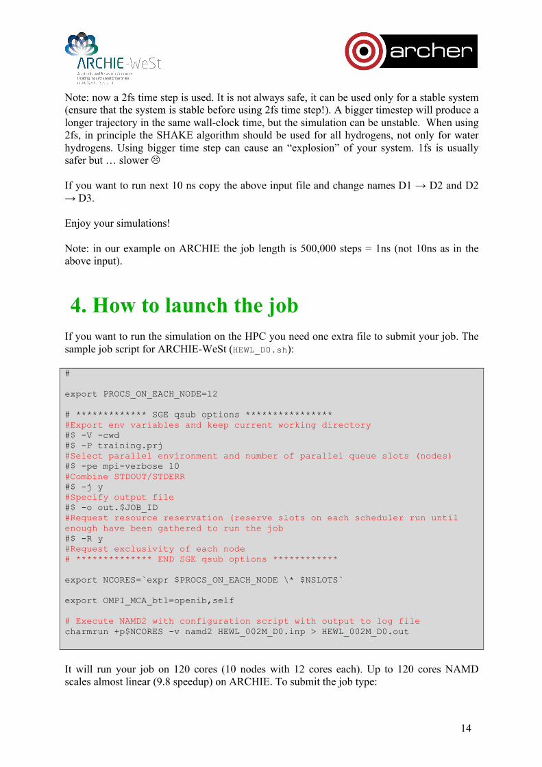
4. How to launch the job If you want to run the simulation on the HPC you need one extra file to submit your job. The sample job script for ARCHIE-WeSt (HEWL_D0.sh): # export PROCS_ON_EACH_NODE=12 # ************* SGE qsub options **************** #Export env variables and keep current working directory #$ -V -cwd #$ -P training.prj #Select parallel environment and number of parallel queue slots (nodes) #$ -pe mpi-verbose 10 #Combine STDOUT/STDERR #$ -j y #Specify output file #$ -o out.$JOB_ID #Request resource reservation (reserve slots on each scheduler run until enough have been gathered to run the job #$ -R y #Request exclusivity of each node # ************** END SGE qsub options ************ export NCORES=`expr $PROCS_ON_EACH_NODE \* $NSLOTS` export OMPI_MCA_btl=openib,self # Execute NAMD2 with configuration script with output to log file charmrun +p$NCORES -v namd2 HEWL_002M_D0.inp > HEWL_002M_D0.out

It will run your job on 120 cores (10 nodes with 12 cores each). Up to 120 cores NAMD scales almost linear (9.8 speedup) on ARCHIE. To submit the job type:

15

qsub HEWL_D0.sh

to check the status type: qstat

To check the calculation progress see the output file (HEWL_002M_D0.out) To run trajectories D0, D1 and D2 one after other the end of the above use HEWL_D0_D2.sh script: … # Execute NAMD2 with configuration script with output to log file charmrun +p$NCORES -v namd2 HEWL_002M_D0.inp > HEWL_002M_D0.out charmrun +p$NCORES -v namd2 HEWL_002M_D1.inp > HEWL_002M_D1.out charmrun +p$NCORES -v namd2 HEWL_002M_D2.inp > HEWL_002M_D2.out Note: The job script is HPC-specific. To run NAMD on ARCHER or other HPC you would need to modify it. If you want to run simulation on your local computer, you would need a file called nodelist: group main host localhost

To run the job type in the terminal: ./run_namd.bash HEWL_002M_D0

6. How to analyze the trajectory

1) visual analysis 2) calculate rmsd and rmsf using the tcl script provided (root mean square distance and

fluctuations of particular residues, respectively) 3) measure distances during the trajectories (for details see vmd tutorial) 4) write your own tcl scripts

16

C. Advanced Simulations

1. PME To see how to use Particle Mesh Ewald method for calculating electrostatic interactions in our case study see files: HEWL_002M_PME_D0.inp, HEWL_002M_PME_D0.inp and HEWL_002M_PME_D0.inp. Lines like the following have appeared: PME yes PMEGridsizex 60 PMEGridsizey 53 PMEGridsizez 59

Note the numbers given should be not smaller than basic cell vectors (cellBasisVector). The PME grid size should be a number which can be produced by adding or multiplying (or both) numbers 2, 3 and 5. In our case cellBasisVector1 was 59.43600082397461, so we need to produce number ~60 (3x5x2x2=60), cellBasisVector2 was 52.60499572753906 (2x3x2x2x2+5=53), cellBasisVector3 was 58.24599838256836 (3x3x2x3+5=59)

2. SMD

a) Constant velocity pulling In this case again we need a SMD file, which should be created basing on the original *SC*pdb file. Again we will pull only one atom CZ from residue ARG128 cp HEWL_002M_SC.pdb HEWL_002M_SMD.pdb HEWL_002M_SMD.pdb: … ATOM 1930 NE ARG P 128 -17.843 -1.453 -18.235 0.00 0.00 PRO N ATOM 1931 HE ARG P 128 -18.195 -1.709 -19.143 0.00 0.00 PRO H ATOM 1932 CZ ARG P 128 -18.593 -1.453 -17.171 1.00 0.00 PRO C ATOM 1933 NH1 ARG P 128 -18.147 -1.043 -15.996 0.00 0.00 PRO N ATOM 1934 HH11 ARG P 128 -18.730 -1.076 -15.196 0.00 0.00 PRO H

… In this file change the occupancy values for all normal atoms to 0.00. The occupancy value 1.00 indicates the SMD atom. HEWL_002M_D2_v0005Aps.inp: structure HEWL_002M_SC.psf coordinates HEWL_002M_SC.pdb bincoordinates HEWL_002M_PME_D1.coor

17

paratypecharmm on parameters par_all27_prot_surf_na.inp exclude scaled1-4 1-4scaling 1.0 switching on switchdist 8 cutoff 12 pairlistdist 14 margin 0 stepspercycle 20 wrapWater on wrapAll on rigidBonds water timestep 2.0 outputenergies 100 outputtiming 100 binaryoutput yes outputname HEWL_002M_D2_v0005Aps dcdfreq 200 restartfreq 100000 restartname rest_HEWL_002M_D2_v0005Aps binvelocities HEWL_002M_PME_D1.vel SMD on SMDFile HEWL_002M_SMD.pdb SMDk 4 SMDVel 0.00001 SMDDir 0.0 0.0 1.0 SMDOutputFreq 100 langevin on langevinDamping 5 langevinTemp 300 langevinHydrogen no extendedSystem HEWL_002M_PME_D1.xsc run 5000000

In this case the pulling velocity has to be specified in the input file – parameter SMDVel. Value 1x10-5 indicates that the pulling velocity is 10-5 A/step. The step is 2fs, so the velocity is 5x10-3 A/ps. The total trajectory length is 10ns, so the atom should move by 50 A during the trajectory. SMDk specifies the spring constant, from my experience 4 is the best value. Sample output: HEWL_002M_PME_D2_v0005Aps.out … WRITING COORDINATES TO DCD FILE AT STEP 499800 The last position output (seq=499800) takes 0.001 seconds, 309.785 MB of memory in use TIMING: 499800 CPU: 2004.69, 0.0042082/step Wall: 2004.69, 0.0042082/step, 0.000233789 hours remaining, 309.785156 MB of memory in

18

use. ENERGY: 499800 813.0956 1119.8652 641.3451 66.5502 -58379.7599 4427.1856 0.0000 0.0000 10249.3769 -41062.3413 300.0943 -51311.7182 -40987.6851 299.7518 343.5534 311.7697 158153.2920 350.8725 349.1137 # Timestep Atom Coordinates force SMD 499900 -10.7265 -1.48513 -11.9009 -0 0 -75.3415 TIMING: 499900 CPU: 2005.09, 0.00398227/step Wall: 2005.09, 0.00398227/step, 0.000110619 hours remaining, 309.785156 MB of memory in use. ENERGY: 499900 790.4483 1107.3516 645.1351 63.4061 -58390.6894 4438.7077 0.0000 0.0000 10272.2767 -41073.3640 300.7648 -51345.6407 -40992.6688 300.4989 291.3132 310.8214 158153.2920 335.7182 338.0513 …

b) Constant force pulling In this example we will use the results from the adsorption trajectory. It means that initially the HEWL protein was placed in the system containing the mica surface model and 90ns trajectory was calculated. During that trajectory the protein adsorbed onto the surface (adsorption trajectory) and the last stage is treated as a starting structure for constant force pulling trajectory (desorption trajectory). It means that the structure after 90ns of adsorption trajectory was saved (under vmd) then water, surface and ions were again added and the system was centered. It means that files: O1_90ns_002M_v0_SC.psf and O1_90ns_002M_v0_SC.pdb were obtained. Then the trajectory D0 was run to minimize the water. Therefore we have files O1_90ns_002M_v0_D0.coor, O1_90ns_002M_v0_D0.xsc, O1_90ns_002M_v0_D0.vel and O1_90ns_002M_v0_D0.dcd (the last two files are not needed for the SMD simulation). Note – the preparation stages are not included in the example. In general we can address the problem that we have: O1_90ns_002M_v0_SC.psf,

O1_90ns_002M_v0_SC.pdb, O1_90ns_002M_v0_D0.coor and O1_90ns_002M_v0_D0.xsc files and we want to run SMD trajectory with constant force pulling. First we have to create the pdb file which will contain information about pulled atoms (the constant force file or SMD file). Copy your *SC*pdb file with other name: cp O1_90ns_002M_v0_SC.pdb O1_90ns_002M_v0_force_f800pN.pdb The new file requires some changes. Let’s assume we want to pull ARG128 CZ atom in the z direction with the force 800pN (11.54 kcal/mol). The most interesting part of the O1_90ns_002M_v0_force_f800pN.pdb file: O1_90ns_002M_v0_force_f800pN.pdb … ATOM 1929 HD2 ARG A 128 21.098 -6.897 -27.912 0.00 0.00 BIA H ATOM 1930 NE ARG A 128 20.244 -8.259 -29.183 0.00 0.00 BIA N ATOM 1931 HE ARG A 128 20.153 -9.222 -28.935 0.00 0.00 BIA H ATOM 1932 CZ ARG A 128 0.000 0.000 1.000 11.54 1.00 BIA C ATOM 1933 NH1 ARG A 128 21.059 -7.038 -30.984 0.00 0.00 BIA N ATOM 1934 HH11 ARG A 128 21.195 -7.096 -32.010 0.00 0.00 BIA H

19

ATOM 1935 HH12 ARG A 128 20.604 -6.238 -30.648 0.00 0.00 BIA H ATOM 1936 NH2 ARG A 128 21.276 -9.260 -30.989 0.00 0.00 BIA N … In this file the information of which atom (atoms) has to be pulled, what is the force value and direction is stored. The last column (B column, green circle) value is equal to 0.00 for all normal atoms. Value 1.00 indicates that the force will be applied to the atom. The occupancy column (orange circle) value is 0.00 for all normal atoms. In the case of the SMD atom it specifies the force value (in kcal/mol, 1kcal/mol=69.479pN). The (x,y,z) columns (blue circle) stores x,y,z coordinates of normal atoms and (x1,y1,z1) coordinates of the force vector in the case of the SMD atom. (x0,y0,z0) coordinates of the force vector are = and (x,y,z) coordinates of the SMD atom (stored in O1_90ns_002M_v0_SC.pdb file, as coordinates of all other atoms). The program will read only rows with B value 1.00 and will omit all rows with B value 0.00. The SMD sample input to the production trajectory D2: HEWL_002M_PME_D2_f100pN.inp: structure O1_90ns_002M_v0_SC.psf coordinates O1_90ns_002M_v0_SC.pdb bincoordinates O1_90ns_002M_v0_D0.coor paratypecharmm on parameters par_all27_prot_surf_na.inp exclude scaled1-4 1-4scaling 1.0 switching on switchdist 8 cutoff 12 pairlistdist 14 margin 0 stepspercycle 20 wrapWater on rigidBonds water timestep 2.0 outputenergies 100 outputtiming 100 binaryoutput yes outputname O1_90ns_002M_v0_sD2_f800pN dcdfreq 100 restartfreq 100000 restartname rest_O1_90ns_002M_v0_sD2_f800pN binvelocities O1_90ns_002M_v0_D0.vel constantforce yes consforcefile O1_90ns_002M_v0_force_f800pN.pdb SMDOutputFreq 100 langevin on

20

langevinDamping 5 langevinTemp 300 langevinHydrogen no extendedSystem O1_90ns_002M_v0_D0.xsc fixedAtoms on fixedAtomsFile O1_90ns_002M_v0_FIX.pdb fixedAtomsCol O minimize 100 run 1000000

Note that to use constant force pulling, 3 new lines, highlighted in red are added. Lines highlighted in purple are needed for the surface which is kept static during the simulation. Note that a short minimization stage is required. To see the result of pulling, watch the trajectory file O1_90ns_002M_v0_sD2_f800pN.dcd

FINAL REMARKS All example files can be found at ARCHIE-WeSt, /users/cwb08102/NAMD_Training

Remember to load modules: /mpi/gcc/openmpi/1.4.5 /libs/gcc/fftw2/float-mpi/2.1.5 /apps/gcc/namd/mpi/2.8 /apps/bin/vmd/1.9.1

How to load the module: module load /apps/bin/vmd/1.9.1

Modules and job submission scripts slightly differs between HPCs.