Architectures of GNSS/INS Integrations - Theoretical Approach and Practical Tests -

Ch. Kreye*, B. Eissfeller, G. Ameres

Institute of Geodesy and Navigation University FAF Munich

Werner-Heisenberg-Weg 39 D-85577 Neubiberg, Germany

*Phone: +49 89 6004 3553, Fax: +49 89 6004 3019, E-Mail: christian.kreye@unibw-muenchen.de

1 Abstract Today integrated GNSS/INS systems are used for many applications in navigation and geodesy. Based on the

complementary error behaviour of both sensors higher performance levels are possible. But the gain in accuracy,

availability, integrity and continuity depends also on the architecture of integration. Following the US view and

discussions the possible methods are separated into three different types called “loose-”, “tight-“ and “deep-

coupling”.

After a short introduction the paper deals firstly with the definition and description of GNSS/INS coupling

principles. In a more theoretical approach the typical characteristics are mentioned. Furthermore the individual

processing algorithms and data flows are presented and compared to each other. In this context also models for

the realisation of the deep coupling principle are derived, driven by the correlator signals of the GNSS receiver.

In a next step the properties of the different architectures are used to assign the main navigation applications to

the mentioned coupling principles.

A simulation tool representing the aiding of INS sensors with GNSS raw data allows investigations about the

error behaviour of this kind of integration. Results of different scenarios varying the type of inertial sensor, the

satellite constellation and the navigation environment enable a detailed evaluation of the potential application

fields.

The more practical part of the paper gives an overview about the different realisations of GNSS/INS integration

at the University FAF Munich and presents current results of simulation programs and field tests in static, car

and aircraft environments. According to the “loose-coupling” principle at first design and navigation results of a

GNSS/IMU attitude system are presented. As an example for high precision positioning a system developed for

determination of railway tracks combining differential carrier-phase GNSS, high precision INS and ultra-sonic

sensors are discussed. An integration on acceleration level is implemented in an airborne vector gravimetry

system using numerous GNSS observations and inertial raw data. Some results of current flight tests give an

overview about the expected system performance.

Finally the design and implementation of a “tightly-coupled” GNSS/INS system is demonstrated. Using

simulation algorithms and results of practical tests in a car navigation environment the advantages but also

difficulties of this method are highlighted.

A conclusion sums up the possibilities of modern GNSS/INS integration techniques.

2 Introduction According to its measurement principle INS systems provide an autonomous solution for position, velocity and

attitude with high data rate and bandwidth. From this point of view an inertial sensor is the optimal choice for

most of the applications in navigation and positioning. Its typical error behaviour, however, causes only a short-

term stability of a high accuracy level. In opposite to that the properties of GNSS systems as another possible

navigation system are completely different. In this case the user depends on a complex ground and space

infrastructure, but the solution is characterized by a long-time error stability and a high accuracy level.

Additionally timing requirements can be fulfilled. These are the main reasons for the successful use of integrated

GNSS/INS systems in many applications providing a higher performance level in comparison to the stand-alone

solutions.

Furthermore for the combination of GNSS and INS measurements the different types of raw data must be taken

into account. On one hand GNSS receivers provide code and phase observations or Doppler frequency offsets to

all satellites in view. In a next step the user position and velocity can be derived based on the known satellite

orbits. On the other hand strapdown inertial sensors measure three dimensional specific forces and angular rates

concerning defined sensor axes. Known initial values of position and velocity as well as sophisticated alignment

algorithms and gravity field reductions allow a real-time update of position, velocity and attitude by integration

of observed accelerations. Thereby error behaviour, type of raw data and required processing steps influence the

navigation performance of each sensor, which can be expressed in the categories of accuracy, availability,

integrity and continuity. In a coupled system the sensors compensate the disadvantages of each other. A better

navigation solution can be provided.

Depending on the application requirements different coupling architectures must be taken into account,

emphasizing also different properties of the provided navigation solution. These integration principles are

presented in the next chapter.

3 Architectures of GNSS/INS Integration

3.1 Loose Coupling Most of GNSS/INS integrations are loosely coupled, giving a great deal of performance in return for simplicity

of integration. In this case the sensors theirselves are completely independent of each other. Using inertial data

beside of initial conditions a so called strapdown computation generates the current INS solution for position,

velocity and attitude. Following the positioning approach also the GNSS systems provides a navigation result

containing position, velocity and time in case of multi-antenna systems also attitude using a Kalman filter

algorithm. Both solutions are combined by a second integrated Kalman filter providing on the one hand

estimations of integrated navigation solution and on the other hand current error states of the inertial sensor like

biases or scale factors. These errors are used in a recursive manner to improve the accuracy of the inertial

navigation solution.

KalmanFilter

GNSS Receiver

PVA

PVA

PV(A)KalmanFilter

InertialNavigation System

NavigationProcessor

INSErrors

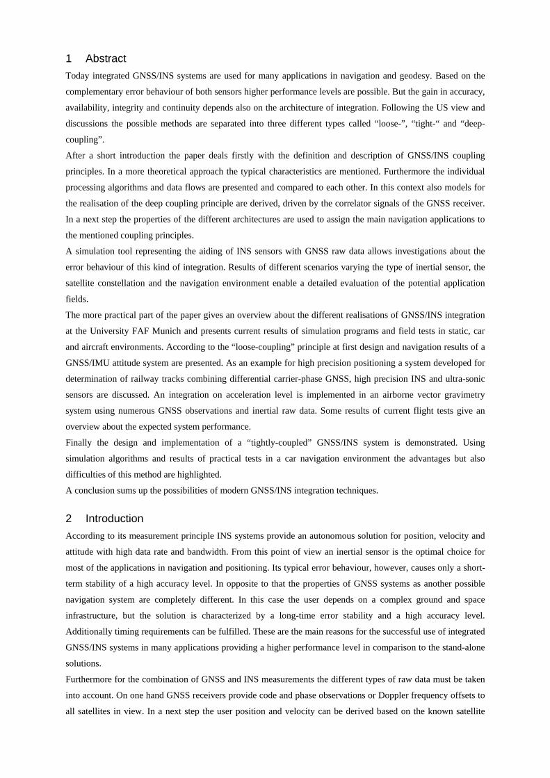
Figure 1: Loose coupling principle (position approach)

A corresponding error and observation model can be described as:

GPSINS

GPSINSINSGPS

INSINSINSINSINS

εεδ

ε

+=+−=−=

+=

HxlLLLl

GxFx& (1)

where: x INS state vector containing navigation and sensor errors F INS dynamics matrix G INS noise input matrix ε sensor noise l linear observation vector L vector of navigation results (position, velocity, attitude or P-V-A) H observation matrix It is straight forward that by integration on P-V level the observation matrix H is diagonal and could be a unit

matrix, depending on the choice of coordinates. A disadvantage of this method is the cascaded structure of two

Kalman filters. Following equation 1 the time-correlations between the GNSS positioning and velocity results

have to be taken into account by some method: either the update time interval is made larger as time correlation-

time constant or the time-correlations are modelled by coloured noise, which however leads to a bigger state

vector. Otherwise the integration processing results in a sub-optimal estimation procedure.

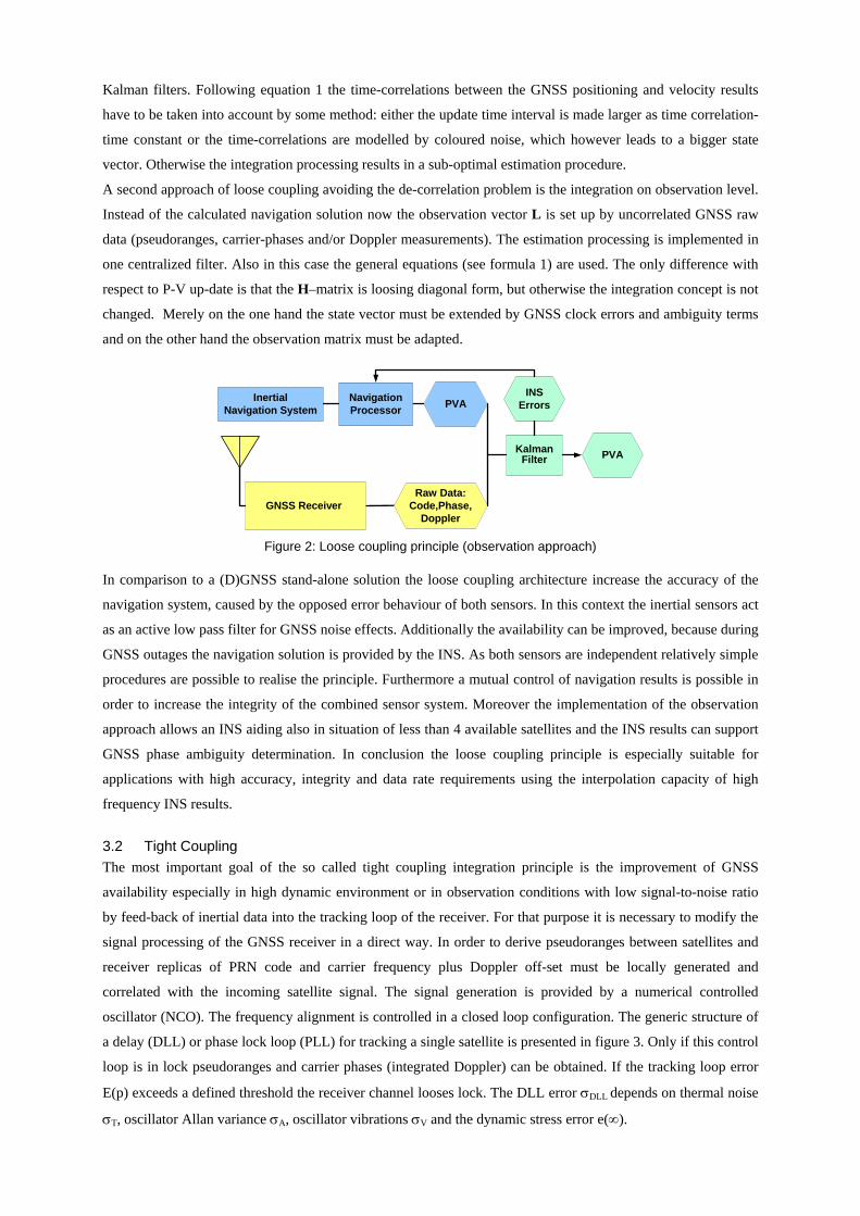
A second approach of loose coupling avoiding the de-correlation problem is the integration on observation level.

Instead of the calculated navigation solution now the observation vector L is set up by uncorrelated GNSS raw

data (pseudoranges, carrier-phases and/or Doppler measurements). The estimation processing is implemented in

one centralized filter. Also in this case the general equations (see formula 1) are used. The only difference with

respect to P-V up-date is that the H–matrix is loosing diagonal form, but otherwise the integration concept is not

changed. Merely on the one hand the state vector must be extended by GNSS clock errors and ambiguity terms

and on the other hand the observation matrix must be adapted.

KalmanFilter

GNSS Receiver

PVA

PVA

Raw Data:Code,Phase,

Doppler

InertialNavigation System

NavigationProcessor

INSErrors

Figure 2: Loose coupling principle (observation approach)

In comparison to a (D)GNSS stand-alone solution the loose coupling architecture increase the accuracy of the

navigation system, caused by the opposed error behaviour of both sensors. In this context the inertial sensors act

as an active low pass filter for GNSS noise effects. Additionally the availability can be improved, because during

GNSS outages the navigation solution is provided by the INS. As both sensors are independent relatively simple

procedures are possible to realise the principle. Furthermore a mutual control of navigation results is possible in

order to increase the integrity of the combined sensor system. Moreover the implementation of the observation

approach allows an INS aiding also in situation of less than 4 available satellites and the INS results can support

GNSS phase ambiguity determination. In conclusion the loose coupling principle is especially suitable for

applications with high accuracy, integrity and data rate requirements using the interpolation capacity of high

frequency INS results.

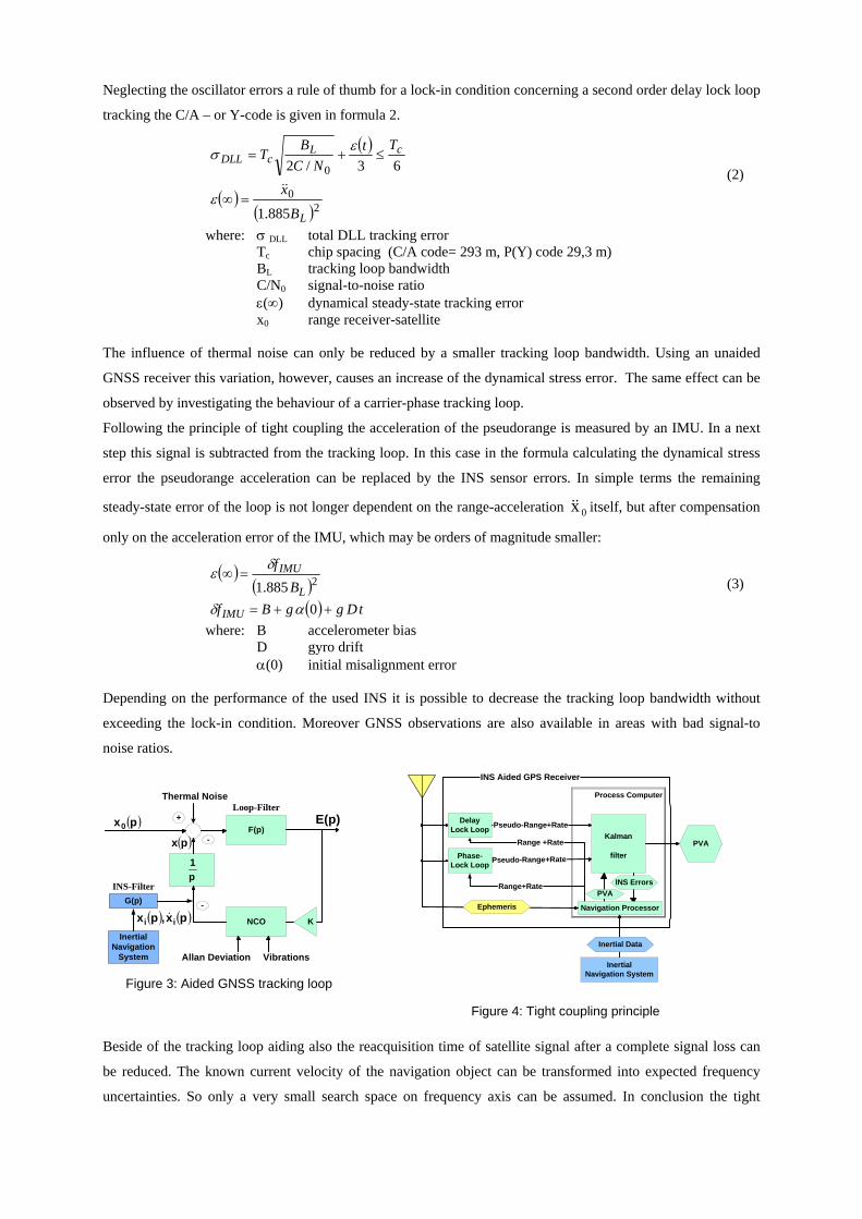
3.2 Tight Coupling The most important goal of the so called tight coupling integration principle is the improvement of GNSS

availability especially in high dynamic environment or in observation conditions with low signal-to-noise ratio

by feed-back of inertial data into the tracking loop of the receiver. For that purpose it is necessary to modify the

signal processing of the GNSS receiver in a direct way. In order to derive pseudoranges between satellites and

receiver replicas of PRN code and carrier frequency plus Doppler off-set must be locally generated and

correlated with the incoming satellite signal. The signal generation is provided by a numerical controlled

oscillator (NCO). The frequency alignment is controlled in a closed loop configuration. The generic structure of

a delay (DLL) or phase lock loop (PLL) for tracking a single satellite is presented in figure 3. Only if this control

loop is in lock pseudoranges and carrier phases (integrated Doppler) can be obtained. If the tracking loop error

E(p) exceeds a defined threshold the receiver channel looses lock. The DLL error σDLL depends on thermal noise

σT, oscillator Allan variance σA, oscillator vibrations σV and the dynamic stress error e(∞).

Neglecting the oscillator errors a rule of thumb for a lock-in condition concerning a second order delay lock loop

tracking the C/A – or Y-code is given in formula 2.

( )

( )( )2

0

0

885.1

63/2

L

cLcDLL

B

x

TtNC

BT

&&=∞

≤+=

ε

εσ (2)

where: σ DLL total DLL tracking error Tc chip spacing (C/A code= 293 m, P(Y) code 29,3 m) BL tracking loop bandwidth C/N0 signal-to-noise ratio ε(∞) dynamical steady-state tracking error x0 range receiver-satellite The influence of thermal noise can only be reduced by a smaller tracking loop bandwidth. Using an unaided

GNSS receiver this variation, however, causes an increase of the dynamical stress error. The same effect can be

observed by investigating the behaviour of a carrier-phase tracking loop.

Following the principle of tight coupling the acceleration of the pseudorange is measured by an IMU. In a next

step this signal is subtracted from the tracking loop. In this case in the formula calculating the dynamical stress

error the pseudorange acceleration can be replaced by the INS sensor errors. In simple terms the remaining

steady-state error of the loop is not longer dependent on the range-acceleration 0x&& itself, but after compensation

only on the acceleration error of the IMU, which may be orders of magnitude smaller:

( )( )

( ) tDggBfB

f

IMU

L

IMU

++=

=∞

0885.1 2

αδ

δε (3)

where: B accelerometer bias D gyro drift α(0) initial misalignment error

Depending on the performance of the used INS it is possible to decrease the tracking loop bandwidth without

exceeding the lock-in condition. Moreover GNSS observations are also available in areas with bad signal-to

noise ratios.

NCO

F(p)+

-

K

Allan Deviation

Loop-Filter

Vibrations

E(p)( )px0

p1

( )px

Thermal Noise

InertialNavigation

System

G(p) -( ) ( )px,px ii &

INS-Filter

Figure 3: Aided GNSS tracking loop

Process Computer

Kalman

filter

Navigation Processor

Inertial Data

PVAINS Errors

InertialNavigation System

DelayLock Loop

Pseudo-Range+Rate

INS Aided GPS Receiver

PVA

Ephemeris

Pseudo-Range+Rate

Phase-Lock Loop

Range +Rate

Range+Rate

Figure 4: Tight coupling principle

Beside of the tracking loop aiding also the reacquisition time of satellite signal after a complete signal loss can

be reduced. The known current velocity of the navigation object can be transformed into expected frequency

uncertainties. So only a very small search space on frequency axis can be assumed. In conclusion the tight

coupling principle especially fulfils the requirements of high dynamic applications. In comparison to lower

coupling levels the anti-jamming capability and availability of the integrated system is improved.

An overview about possible loop and signal parameters that allow stable tracking operation according to

equation 2 is presented in table 1. Development history has shown that tight coupling in real world is not so

efficient as it was expected: There is always a lever arm between antenna and IMU causing differences in

applied acceleration fields. Closing the loop bandwidth implies a higher performance oscillator.

System design INS category (drift, bias)

Effective g [m/s²]

Bandwidth BL [Hz]

Min. C/N0 [dB-Hz]

DLL unaided N/A 90 2.0 20 DLL+ MEMS INS 10°/h, 1 mg 0.4 0.2 7.3 DLL+ FOG INS 1°/h, 0.1 mg 0.04 0.06 2.3 DLL+ RLG INS 0.01°/h, 0.01 mg 0.004 0.02 -2.6

Table 1: P(Y) -code tracking loop performance using inertial aiding

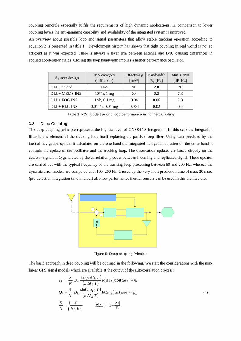
3.3 Deep Coupling The deep coupling principle represents the highest level of GNSS/INS integration. In this case the integration

filter is one element of the tracking loop itself replacing the passive loop filter. Using data provided by the

inertial navigation system it calculates on the one hand the integrated navigation solution on the other hand it

controls the update of the oscillator and the tracking loop. The observation updates are based directly on the

detector signals I, Q generated by the correlation process between incoming and replicated signal. These updates

are carried out with the typical frequency of the tracking loop processing between 50 and 200 Hz, whereas the

dynamic error models are computed with 100–200 Hz. Caused by the very short prediction time of max. 20 msec

(pre-detection integration time interval) also low performance inertial sensors can be used in this architecture.

p1

Figure 5: Deep coupling Principle

The basic approach in deep coupling will be outlined in the following. We start the considerations with the non-

linear GPS signal models which are available at the output of the autocorrelation process:

( )( ) ( ) ( )

( )( ) ( ) ( )

( )cT

L

kkkk

kkk

kkkk

kkk

RBN

CNS

RTf

TfD

NSQ

RTf

TfD

NSI

ττ

ξϕτππ

ηϕτππ

∆−=∆=

+∆∆∆∆

=

+∆∆∆∆

=

1

sinsin

cossin

0

(4)

where I , Q in-phase, quadra-phase signal component S/N signal-to-noise ratio C/N0 carrier-to-Noise ratio in 1 Hz bandwidth BL single-sided noise bandwidth of the tracking loop Dk navigation data bit R(∆τk) autocorrelation function des C/A oder P(Y)- codes: Tc chip-length of the code-chip ∆fk frequency error ∆τk synchronization (range error) error ∆ϕk carrier-phase error ηk,ξk noise components (AWGN), E{ηk}= E{ξk}=0, E{ηk2}= E{ξk2}=1 T coherent integration time intervall (T = 0.020 s, typically) k discrete time

The signal expressions are highly non-linear, which leads in some implementations to the application of the

Extended Kalman filter. Alternatively, a linearization is possible by linearization at an operation point or by

applying additional mathematical functions on the signals in order to remove some non-linearities (conventional

detectors). The next step is then to relate the I and Q components to the position and velocity error states:

⎟⎟⎠

⎞⎜⎜⎝

⎛∆+∆

∂∂

+∆∂∂

+∆∂∂

+∆∂∂

+∆∂∂

+∆∂∂

−≅∆

⎟⎟⎠

⎞⎜⎜⎝

⎛∆++∆

∂∂

+∆∂∂

+∆∂∂

≅∆

∆+∆∂∂

+∆∂∂

+∆∂∂

≅∆

kkk

kk

k

kk

k

kk

k

kk

k

kk

k

kk

kkkk

kk

k

kk

k

kk

kkk

kk

k

kk

k

kk

Czz

yy

xx

zz

yy

xxc

ff

CBzz

yy

xx

Czz

yy

xx

&&&

&&

&

&&

&

&&&& ττττττ

τττθ

ττττ

λπ2 (5)

This means from each tracked satellite we get in minimum a pair of I and Q observations, which contain

information about the position, velocity, clock and carrier ambiguity states. These observations are then

combined with a dynamic error model of the IMU error states. In a linear or non-linear Kalman filter

formulation the unknowns are estimated. Thus, all tracking loops are processed in a parallel unified process.

Based on the estimated unknowns the tracking loop corrections ∆fk , ∆τk, ∆ϕk are re-computed and are applied to

the current operation points of the correlators, with the effect of improved time and frequency synchronization

between the received signal and the local replicas. The main advantages are that each tracking loop of the

receiver is not independent any longer (Vector Delay Lock Loop) on a single satellite as it is the case of a

conventional receiver. Even in the case of small S/N – ratio, e.g. by jamming or interference, for a specific

satellite feed-back or steering command values for the loop can still be generated and the loop doesn’t loose lock

very early. Deep coupling can be considered as real signal aiding. The improvement in anti-jam is more as 10

dB with respect to tight coupling, but is very difficult to assess.

4 Simulation of aided Inertial Navigation The presented tool simulates an INS loosely coupled with GNSS range and range rate measurements. INS

specification parameters (see table 2), satellite orbit information, GNSS antenna patterns and the user trajectory

are read from simple ASCII-files. Based on this information, navigation and sensor errors are estimated in a

Kalman filter as described in the following.

Based on the latitude of the user, a fine alignment is simulated, using typical coarse alignment angles of the

specific INS. With the achieved angles and their accuracy the navigation starts. Height stabilization is done by

implementation of a conventional baro-inertial loop.

The basic element of the Kalman filter is the standard Schmidt dynamics matrix. This matrix is extended to

estimate instrument errors and furthermore GNSS clock errors. The according state-vector contains 24 elements.

To control instrument noise a sensor noise vector and its spectral density matrix with sensor-typical values are

set up along with a noise input matrix, which maps the sensor noise to values in the state vector and its

covariance matrix.

Figure 6: Effects of a fixed gyro bias (1°/h)

Parameter Value, (Correlation time) Random-Walk Gyro h00150 o /.

Accelerometer noise 5 µg, (Kalman cycle) Gyro drift 0.003o/h, 3600 s Gyro scale factor 0.2 ppm, 3600 s Accelerometer bias 25 µg, 3600 s Accelerometer scale factor 120 ppm, 3600 s

Table 2: Simulated INS errors

Without GNSS updates the Kalman filter only predicts the navigation errors. An example is given in figure 6.

Effects of Schuler- and Foucault-frequency as well as the earth rotation rate can be verified.

If GNSS data is available the filter performs an update. In this case the observation vector contains differences in

ranges and range rates based on GNSS measurements and current navigation parameters. The GNSS

observations are obtained by simulating a dual frequency receiver using standard error models for tropospheric

and ionospheric influences on the signal, satellite orbits and tracking loop noise. For each observation a standard

deviation is estimated.

Simulations were performed with performance parameters of an LN-100 and an LN-200. The results of the static

user without GPS aiding show characteristics and limitations of the used INS. Figure 7 presents the propagation

of the latitude velocity error of the simulated LN-100 INS. The error is oscillating within its RMS band. In figure

8 the long-term stability of the corresponding GNSS error is demonstrated. Using the integrated system the

accuracy can be increased to the level of 1 cm/s.

Figure 7: Latitude velocity (free-running INS)

Figure 8: Integrated latitude velocity

Various simulations were carried out using different dynamical conditions (e.g. static user, car and aircraft

environment). Especially the improved observability of INS sensor error in case of high dynamics must be

pointed out. This behaviour is confirmed in figure 9 and 10 representing the estimation of accelerometer errors.

During high dynamic aircraft manoeuvres the RMS error is reduced significantly.

Figure 9: Accelerometer bias (dynamic case)

Figure 10: Accelerometer scale factor (dynamic case)

5 Practical Implementations

5.1 Attitude Determination Using multi-antenna systems GNSS provides also attitude solutions based on the interferometric principle. The

accuracy depends on the baseline length between reference and rover antennas. If an application allows only

short baseline lengths GNSS errors like receiver noise and multipath effects degrade the accuracy of the attitude

solution. Moreover GNSS outages yield in some applications to numerous periods without any navigation result.

Another problem is the integrity of the system. Errors in the ambiguity determination after a signal reacquisition

cause wrong attitude results. Using GNSS stand-alone systems the user is not able to detect the system

instability. In this context some investigations are carried out with a NOVATEL Beeline two-antenna system and

a DQI MEMS IMU (gyro drift 20°/h) in static and dynamic environments (see figure 11). Varying satellite

constellation, baseline length and observation environment the performance of the loosely coupled system in

comparison to the GNSS results is evaluated.

-0.30

-0.25

-0.20

-0.15

-0.10

200318 200443 200568 200693 200818

GPS-Lösung GPS/INS-Lösung

elevationin [°]

GPS-timein [s]

-0.30

-0.25

-0.20

-0.15

-0.10

200318 200443 200568 200693 200818

GPS-Lösung GPS/INS-Lösung

elevationin [°]

GPS-timein [s]

-0.30

-0.25

-0.20

-0.15

-0.10

200318 200443 200568 200693 200818

GPS-Lösung GPS/INS-Lösung

elevationin [°]

GPS-timein [s]

-0.30

-0.25

-0.20

-0.15

-0.10

200318 200443 200568 200693 200818

GPS-Lösung GPS/INS-Lösung

elevationin [°]

GPS-timein [s]

Figure 11: Test configuration of GNSS/INS attitude determination

As presented in the graph of figure 11 the total effects of receiver noise are nearly eliminated in the integrated

result for azimuth and elevation. Also the influence of multipath effects can be reduced if the filter parameters

are adapted to the expected values. With the described category of inertial sensors GNSS outages up to 90

seconds can be bridged without a significant decrease in accuracy. In table 3 an overview of the investigated

attitude performance is presented. It must be emphasized, that a significant improvement is only possible if INS

aiding is provided especially in system availability and data rate. Instead of this an increase in available satellites

in former times with GLONASS in the future with GALILEO shows only small positive effects.

GPS GPS/GLONASS GPS+IMU GPS/GLONASS+IMU Accuracy (6 m baseline)

σ (azimuth) 0.03°-0.05° 0.03°-0.05° 0.01°-0.03° 0.01°-0.03°

Accuracy (6 m baseline σ (elevation) 0.05°-0.08° 0.05°-0.08° 0.02°-0.04° 0.02°-0.04°

Availability + ++ ++++ +++++ Data rate 2-10 Hz 2-10 Hz 100 Hz 100 Hz

Table 3: Performance of attitude results

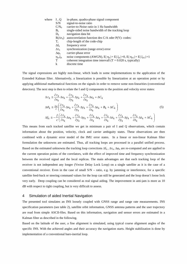
5.2 High Precision Positioning An example for a practical implementation of the loose coupling architecture for high precision positioning is the

track irregularity measurement system (TIMS) developed in the context of our sensor fusion activities. The

system design is based on the integration of differential GPS with an inertial navigation system. The primary

task of the system is to acquire high-precision data for post-processing. To determine the higher dynamics of the

measurement platform, a precise inertial navigation system (SAGEM, Sigma 30) is used. The INS position is

then augmented using carrier phase observations of the differential GPS system to eliminate inertial errors.

Surveying of the rail heads is done by use of ultrasonic sensors in two perpendicular directions. The distance

between platform and rail heads is measured in horizontal and vertical directions. Considering attitude and

position of the platform determined by the position system and known lever arms between all system

components, the absolute position of both railheads can be derived. Pictures of the system design are given in

figure 12.

Figure 12: System design for railway measurements

Based on computed railhead positions the geometric line characteristics of the investigated track can be derived.

Examples are the curvature, the cross-level, defined as the vertical height difference between left and right track

and the distance between both tracks called gauge. In the scope of this project practical test were carried out on a

test track of 20 km in Austria in cooperation with the Austrian railway company ÖBB. Considering a train speed

of 30 km/h a position resolution of 20 cm is feasible. The following graphs show some results of this

measurement campaign. In figure 13 an example of the continuously derived positions, INS barycentre and

railheads, is presented. Figure 14 demonstrates the changes in gauge and cross-level along the test track. The

height difference during curve areas is detected very significant. The synchronous expansion of the gauge can be

interpreted as mechanical wear of the track.

48.07650

48.07655

48.07660

48.07665

48.07670

48.07675

48.07680

48.07685

15.59478 15.59479 15.59480 15.59481

Latit

ude

Longitude

x374737.29

x374739.97

Trajectorie of INS BarycenterRailhead

48.07650

48.07655

48.07660

48.07665

48.07670

48.07675

48.07680

48.07685

15.59478 15.59479 15.59480 15.59481

Latit

ude

Longitude

x374737.29

x374739.97

Trajectorie of INS BarycenterRailhead

Figure 13: Observation results Figure 14: Derived values for railway applications

In summary the described railway application is a verification of the high accuracy potential of loosely coupled

GNSS/INS integrations.

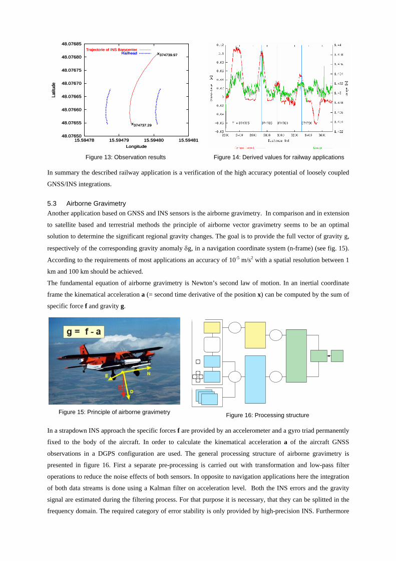
5.3 Airborne Gravimetry Another application based on GNSS and INS sensors is the airborne gravimetry. In comparison and in extension

to satellite based and terrestrial methods the principle of airborne vector gravimetry seems to be an optimal

solution to determine the significant regional gravity changes. The goal is to provide the full vector of gravity g,

respectively of the corresponding gravity anomaly δg, in a navigation coordinate system (n-frame) (see fig. 15).

According to the requirements of most applications an accuracy of 10-5 m/s2 with a spatial resolution between 1

km and 100 km should be achieved.

The fundamental equation of airborne gravimetry is Newton’s second law of motion. In an inertial coordinate

frame the kinematical acceleration a (= second time derivative of the position x) can be computed by the sum of

specific force f and gravity g.

Figure 15: Principle of airborne gravimetry

Figure 16: Processing structure

In a strapdown INS approach the specific forces f are provided by an accelerometer and a gyro triad permanently

fixed to the body of the aircraft. In order to calculate the kinematical acceleration a of the aircraft GNSS

observations in a DGPS configuration are used. The general processing structure of airborne gravimetry is

presented in figure 16. First a separate pre-processing is carried out with transformation and low-pass filter

operations to reduce the noise effects of both sensors. In opposite to navigation applications here the integration

of both data streams is done using a Kalman filter on acceleration level. Both the INS errors and the gravity

signal are estimated during the filtering process. For that purpose it is necessary, that they can be splitted in the

frequency domain. The required category of error stability is only provided by high-precision INS. Furthermore

by post-processing algorithms the separation of time-dependent INS errors and space-dependent gravity signal

can be completed using e.g. crossover points in the flight trajectory.

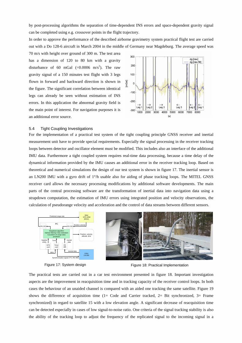
In order to approve the performance of the described airborne gravimetry system practical flight test are carried

out with a Do 128-6 aircraft in March 2004 in the middle of Germany near Magdeburg. The average speed was

70 m/s with height over ground of 300 m. The test area

has a dimension of 120 to 80 km with a gravity

disturbance of 60 mGal (=0.0006 m/s2). The raw

gravity signal of a 150 minutes test flight with 3 legs

flown in forward and backward direction is shown in

the figure. The significant correlation between identical

legs can already be seen without estimation of INS

errors. In this application the abnormal gravity field is

the main point of interest. For navigation purposes it is

an additional error source.

5.4 Tight Coupling Investigations For the implementation of a practical test system of the tight coupling principle GNSS receiver and inertial

measurement unit have to provide special requirements. Especially the signal processing in the receiver tracking

loops between detector and oscillator element must be modified. This includes also an interface of the additional

IMU data. Furthermore a tight coupled system requires real-time data processing, because a time delay of the

dynamical information provided by the IMU causes an additional error in the receiver tracking loop. Based on

theoretical and numerical simulations the design of our test system is shown in figure 17. The inertial sensor is

an LN200 IMU with a gyro drift of 1°/h usable also for aiding of phase tracking loops. The MITEL GNSS

receiver card allows the necessary processing modifications by additional software developments. The main

parts of the central processing software are the transformation of inertial data into navigation data using a

strapdown computation, the estimation of IMU errors using integrated position and velocity observations, the

calculation of pseudorange velocity and acceleration and the control of data streams between different sensors.

Position, velocity,attitude, time

LittonLN-200

Mitel GPS ARM

(RISC)

GPScard

Timercard

RS485

RS 232 RS 232

Strapdown algorithmKalman filtering+ bias estimation

Caculation of range-ratesprediction

Inertialdata

TimeSatelliteorbits

PPSInertial data

Synchronisation signal (TTL-RS 485)

Position,velocity

Predicted range-rate

PC

Figure 17: System design Figure 18: Practical Implementation

The practical tests are carried out in a car test environment presented in figure 18. Important investigation

aspects are the improvement in reacquisition time and in tracking capacity of the receiver control loops. In both

cases the behaviour of an unaided channel is compared with an aided one tracking the same satellite. Figure 19

shows the difference of acquisition time (1= Code and Carrier tracked, 2= Bit synchronized, 3= Frame

synchronized) in regard to satellite 15 with a low elevation angle. A significant decrease of reacquisition time

can be detected especially in cases of low signal-to-noise ratio. One criteria of the signal tracking stability is also

the ability of the tracking loop to adjust the frequency of the replicated signal to the incoming signal in a

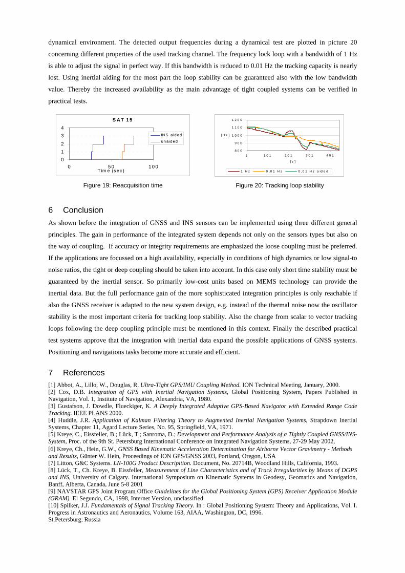
dynamical environment. The detected output frequencies during a dynamical test are plotted in picture 20

concerning different properties of the used tracking channel. The frequency lock loop with a bandwidth of 1 Hz

is able to adjust the signal in perfect way. If this bandwidth is reduced to 0.01 Hz the tracking capacity is nearly

lost. Using inertial aiding for the most part the loop stability can be guaranteed also with the low bandwidth

value. Thereby the increased availability as the main advantage of tight coupled systems can be verified in

practical tests.

S AT 1 5

012

34

0 5 0 1 0 0T im e (s ec )

IN S aidedunaided

Figure 19: Reacquisition time

8 0 0

9 0 0

1 0 0 0

1 1 0 0

1 2 0 0

1 1 0 1 2 0 1 3 0 1 4 0 1

[ s ]

[ H z ]

1 H z 0 , 0 1 H z 0 , 0 1 H z a id e d Figure 20: Tracking loop stability

6 Conclusion As shown before the integration of GNSS and INS sensors can be implemented using three different general

principles. The gain in performance of the integrated system depends not only on the sensors types but also on

the way of coupling. If accuracy or integrity requirements are emphasized the loose coupling must be preferred.

If the applications are focussed on a high availability, especially in conditions of high dynamics or low signal-to

noise ratios, the tight or deep coupling should be taken into account. In this case only short time stability must be

guaranteed by the inertial sensor. So primarily low-cost units based on MEMS technology can provide the

inertial data. But the full performance gain of the more sophisticated integration principles is only reachable if

also the GNSS receiver is adapted to the new system design, e.g. instead of the thermal noise now the oscillator

stability is the most important criteria for tracking loop stability. Also the change from scalar to vector tracking

loops following the deep coupling principle must be mentioned in this context. Finally the described practical

test systems approve that the integration with inertial data expand the possible applications of GNSS systems.

Positioning and navigations tasks become more accurate and efficient.

7 References [1] Abbot, A., Lillo, W., Douglas, R. Ultra-Tight GPS/IMU Coupling Method. ION Technical Meeting, January, 2000. [2] Cox, D.B. Integration of GPS with Inertial Navigation Systems, Global Positioning System, Papers Published in Navigation, Vol. 1, Institute of Navigation, Alexandria, VA, 1980.

[3] Gustafson, J. Dowdle, Flueckiger, K. A Deeply Integrated Adaptive GPS-Based Navigator with Extended Range Code Tracking. IEEE PLANS 2000. [4] Huddle, J.R. Application of Kalman Filtering Theory to Augmented Inertial Navigation Systems, Strapdown Inertial Systems, Chapter 11, Agard Lecture Series, No. 95, Springfield, VA, 1971.

[5] Kreye, C., Eissfeller, B.; Lück, T.; Sanroma, D.; Development and Performance Analysis of a Tightly Coupled GNSS/INS-System, Proc. of the 9th St. Petersburg International Conference on Integrated Navigation Systems, 27-29 May 2002, [6] Kreye, Ch., Hein, G.W., GNSS Based Kinematic Acceleration Determination for Airborne Vector Gravimetry - Methods and Results, Günter W. Hein, Proceedings of ION GPS/GNSS 2003, Portland, Oregon, USA [7] Litton, G&C Systems. LN-100G Product Descripition. Document, No. 20714B, Woodland Hills, California, 1993. [8] Lück, T., Ch. Kreye, B. Eissfeller, Measurement of Line Characteristics and of Track Irregularities by Means of DGPS and INS, University of Calgary. International Symposium on Kinematic Systems in Geodesy, Geomatics and Navigation, Banff, Alberta, Canada, June 5-8 2001 [9] NAVSTAR GPS Joint Program Office Guidelines for the Global Positioning System (GPS) Receiver Application Module (GRAM). El Segundo, CA, 1998, Internet Version, unclassified.

[10] Spilker, J.J. Fundamentals of Signal Tracking Theory. In : Global Positioning System: Theory and Applications, Vol. I. Progress in Astronautics and Aeronautics, Volume 163, AIAA, Washington, DC, 1996. St.Petersburg, Russia