are biogeographic provinces discrete or … · observation of a gradient where provinces have been...
TRANSCRIPT

ARE BIOGEOGRAPHIC PROVINCES DISCRETE OR GRADATIONAL: A TEST IN
THE LATE ORDOVICIAN OF LAURENTIA
by
CHELSEA ELLEN JENKINS
(Under the Direction of Steven M. Holland)
ABSTRACT
Provinces are the standard method of characterizing the spatial distribution
of communities in ecology and biogeography. Provinces do not always exhibit
clear boundaries or homogenous and compellingly distinct compositions. Similar
provinces with spatially meaningful compositional overlap may be divisions along
a biogeographic gradient. Four provinces have been recognized in the Late
Ordovician of Laurentia: Appalachian, Southern, Midcontinent, and Western.
These provinces correspond to geochemically distinct water masses based on
isotopic analysis, and have been documented for several taxonomic groups. Spatial
trends in the Jaccard similarities and ordination scores of faunal communities in
these provinces presented here suggest these provinces are divisions of a
continent-scale gradient driven by siliciclastic input and associated environmental
effects of the Taconic Orogeny. Gradients can be useful in considering faunal
distribution in terms of influential environmental factors and vice versa.

Observation of a gradient where provinces have been inferred suggests gradients
are insufficiently documented in paleobiogeography.
INDEX WORDS: province, gradient, biogeography, Laurentia, Ordovician

ARE BIOGEOGRAPHIC PROVINCES DISCRETE OR GRADATIONAL: A TEST IN
THE LATE ORDOVICIAN OF LAURENTIA
by
CHELSEA ELLEN JENKINS
B.S., College of William & Mary, 2011
A Thesis Submitted to the Graduate Faculty of The University of Georgia in Partial
Fulfillment of the Requirements for the Degree
MASTER OF SCIENCE
ATHENS, GEORGIA
2014

© 2014
Chelsea Ellen Jenkins
All Rights Reserved

ARE BIOGEOGRAPHIC PROVINCES DISCRETE OR GRADATIONAL: A TEST IN
THE LATE ORDOVICIAN OF LAURENTIA
by
CHELSEA ELLEN JENKINS
Major Professor: Steven M. Holland
Committee: Susan T. GoldsteinArnold I. Miller
Electronic Version Approved:
Maureen GrassoDean of the Graduate SchoolThe University of GeorgiaMay 2014

ACKNOWLEDGEMENTS
I am particularly grateful for Steve Holland’s guidance and seemingly
inexhaustible patience throughout the course of this project and my studies at the
University of Georgia. I would also like to thank Arnie Miller and Sue Goldstein for their
time and input while serving on my committee.
I am grateful for the time, expertise, and patience of those who assisted me in the
field: Megan Flansburg, Judi Sclafani, and Allison Platsky. I appreciate prior work by
Mark Patzkowsky in conjunction with Steve Holland, whose data I used alongside my
own in this study. I also thank these generous souls for assistance in finding the oft-
elusive shallow subtidal, fossiliferous, Late Ordovician outcrops in the Appalachians:
Matt Powell, Sean Cornell, Andrew Rindsberg, John Haynes, Roger Thomas, Rick
Diecchio, Bob Ganis, David Brezinski, Bill Kochanov, Thomas Kammer, Karen Layou,
Duff Gold, John Repetski, and Dale Springer.
I also thank the Geological Society of America and the Miriam Watts-Wheeler
Fund for funding this research.
iv

TABLE OF CONTENTS
Page
ACKNOWLEDGEMENTS................................................................................................iv
LIST OF TABLES.............................................................................................................vii
LIST OF FIGURES..........................................................................................................viii
CHAPTER
1 INTRODUCTION.............................................................................................1
2 ARE BIOGEOGRAPHIC PROVINCES DISCRETE OR GRADATIONAL: A
TEST IN THE LATE ORDOVICIAN OF LAURENTIA..................................2
INTRODUCTION.......................................................................................3
BACKGROUND.........................................................................................5
METHODS................................................................................................16
RESULTS..................................................................................................21
DISCUSSION............................................................................................27
CONCLUSIONS........................................................................................33
3 CONCLUSIONS..............................................................................................34
LITERATURE CITED......................................................................................................35
APPENDIX
1 Paleobiology Database Collections Used in the Continent Scale Analysis.....57
2 Collections From Previous Studies Used in the Regional Scale Analysis.......62
3 Faunal Censuses: Appalachian Collections.....................................................63
v

4 Appalachian Field Localities...........................................................................69
5 Similarity Values, Continent Scale and Regional Scale .................................70
6 R-Code.............................................................................................................73
vi

LIST OF TABLES
Page
Table 1: Most abundant taxa in each province during the Early Ordovician ...................44
Table 2: Most abundant taxa in each province during the Middle Ordovician ................45
Table 3: Most abundant taxa in each province during the Late Ordovician......................46
Table 4: Most abundant taxa in each subregion of the Southern and Appalachian
Provinces in the regional scale study ....................................................................47
vii

LIST OF FIGURES
Page
Figure 1: Recognized biogeographic provinces in the Late Ordovician of Laurentia ......48
Figure 2: Map of field localities.........................................................................................49
Figure 3: Stratigraphic distribution of samples .................................................................50
Figure 4: Jaccard's similarity for each combination of provinces in the continent scale
study.......................................................................................................................51
Figure 5: Jaccard's similarity for each combination of subregions in the regional scale
study.......................................................................................................................52
Figure 6: Ordination of collections from the regional scale study.....................................53
Figure 7: Ordination of taxa from the regional scale study...............................................54
Figure 8: Jaccard's similarity vs. distance .........................................................................55
Figure 9: Schematic representation of the proposed gradient in the Late Ordovician of
Laurentia ...............................................................................................................56
viii

CHAPTER 1
INTRODUCTION
This thesis is presented as one chapter, as it is composed in the format of a
manuscript intended for submission to the journal Paleobiology. The second chapter
includes the background, methods, results, discussion, and conclusions. The third chapter
concludes this thesis.
Provinces are used to characterize the spatial distribution of communities in
ecology and biogeography (Wallace 1876; Spalding et al. 2007). Criteria used for
defining provinces varies by focus and by researcher (Ekman 1953; Briggs 1975; Knox
1980). Provincial boundaries are not always discrete. Furthermore, faunal compositions
of adjacent provinces can be similar, and faunal composition is not homogenous across
provinces (Adey and Steneck 2001). Adjacent provinces with similar faunal makeup may
be divisions on a gradient.
Biogeographic provinces are often bounded by changes in environmental
characteristics, and these environmental characteristics vary along gradients (Adey and
Steneck 2001). For this reason, gradients may be useful in considering faunal distribution
directly in terms of variation of important environmental factors.
The purpose of this study is to compare recognized biogeographic provinces in the
Late Ordovician of Laurentia in terms of faunal similarity and spatial patterns in
similarity to determine if distribution patterns are better described by distinct provinces or
as a gradient.
1

CHAPTER 2
ARE BIOGEOGRAPHIC PROVINCES DISCRETE OR GRADATIONAL: A TEST IN
THE LATE ORDOVICIAN OF LAURENTIA1
1Jenkins, C.E., and Holland, S.M. To be submitted to Paleobiology.
2

“Provinces must, to be understood, be traced back, like species, to their history and origins in past time”
Forbes (1859)
Introduction
Biogeographic provinces are often used to describe the spatial organization of
ecology. Provinces are the results of physical, chemical, and biological environmental
factors that limit dispersion (Jablonski et al. 1985). As these factors change spatially and
through time, provinces are dynamic, and because they describe how fauna are organized,
they are considered a fundamental unit in biogeography. The size and number of
provinces through time have implications for diversity, although it is unclear exactly how
much provinciality, rather than community teiring and distance or habitat area, controls
diversity (Valentine et al. 1978; Sepkoski 1988; Miller et al. 2009; Holland 2010).
Provinces are used to guide biotic conservation efforts (Spalding et al. 2007), as
ecological tools in paleobiogeographic studies (Sclafani and Holland 2013), and for
reconstructing paleogeography (McKerrow and Cocks 1986).
Understanding the environmental factors that lead to provinciality promotes better
characterization of faunal distributions. Applying the first tenant of biogeography
suggests that closer locations will be more compositionally similar (Tobler 1970), but this
alone does not describe ecological patterns. Physical boundaries, such as continents or
large expanses of deep ocean often bound provinces, but other boundaries tend not to be
so absolute, such as environmental bounding factors like temperature, salinity, or
substrate (Spalding et al. 2007). There is no reason to expect that these environmental
factors produce discrete boundaries in space. Environmental factors changing along a
3

gradient are familiar (e.g., temperature, pressure, oxygen availability), and biogeographic
provinces often do not have sharp or easily defined boundaries (Adey and Steneck 2001;
Briggs and Bowen 2012). Biogeographic distributions known to be controlled, at least in
part, by these factors could be expected to reflect the controlling gradients. Depending on
the steepness of a gradient, divisions along the gradient, or provinces, may be discernible.
However, if the factors that control the phenomena that provinces describe are of interest,
gradients may be more useful.
Provinces are increasingly being utilized as units for conservation efforts as our
own modern environment changes (Spalding et al. 2007). It is forecasted that the
organization of provinces will become increasingly unstable as climate changes, with
biogeographic provinces variably reacting to the rise or demise of certain key taxa as well
as to the changes in boundary-defining conditions (Hiscock et al. 2004). Null models
suggest climate change will disproportionately affect fauna near provincial boundaries,
owing to the concentration of species occupying the extreme ends of their range (Roy
2001). The Late Ordovician is an ideal time to study the dynamics of provinces and
potential gradients, as it is a time characterized by great and varied environmental change
from Hirnantian glaciation and tropical cooling, as well as the effects of the Taconic
orogeny (Holland and Patzkowsky 1996, 1997).
In the Late Ordovician of Laurentia, four provinces have been recognized: the
Appalachian, Midcontinent (Missouri, upper Mississippi valley, Michigan, to western
Pennsylvania and New York), Southern (Cincinnati Arch and Nashville Dome), and
Western Provinces (New Mexico, Colorado, Wyoming, and most of Canada; Fig. 1).
4

These provinces correspond to geochemically distinct water masses based on isotopic
analysis (Holmden et al. 1998). Faunal distribution patterns in some taxonomic groups
support these provinces, including corals (Elias 1982; Elias 1983; Elias and Young 1998),
conodonts (Sweet and Bergstrom 1974; Barnes and Fahraeus 1975; Bergstrom 1983),
ostracods (Mohibullah et al. 2012), bryozoans (Antsey 1986), and other distinctive trace-
fossil and community assemblages (Jin et al. 2012). These provinces also have distinct
relative abundance distributions as indicated by analysis of Hubbell's theta (Sclafani and
Holland 2013). Given that these provinces may have environmentally driven bounding
factors that operate on a gradient, this study seeks to understand whether provinces
adequately describe spatial patterns in faunal similarity at continental and regional scales
in the Late Ordovician Laurentia, or if these patterns are better described as one or more
gradients.
Background
Provinces.———Provinces have long been a cornerstone of biogeography
(Wallace 1876; Jablonski et al. 1985; Spalding et al. 2007). In the hierarchical
biogeographic area classification system, provinces are nested within realms, which tend
to be continent to subcontinent-sized areas with coherent biotic assemblages at higher
(generic to familial) taxonomic levels (Udvardy 1975). Provinces are a subdivision of
these realms, and are generally delineated at the specific and generic taxonomic levels.
Distinct, coherent suites of fauna at these levels arise from historical isolation and other
abiotic controls, such as geomorphological features, hydrographic features (e.g., currents,
5

upwelling, ice), and geochemical features (e.g., nutrient supply, salinity), where changes
in these factors create boundaries to dispersal (Spalding et al. 2007). The concept of a
province is theoretically straightforward, but the process of defining a province can be
complicated.
Defining Provinces.———Provinces can be defined several ways, depending on
available data. In modern environments, provinces can be delimited with detailed
measurements of temperature, salinity, chemical characteristics, faunal characteristics,
and productivity (Szekielda 2005). Such data may be unattainable in the distant past, so
ancient provinces are usually defined with features observable in the rock record, such as
faunal composition (Briggs 1995), and proxies for environmental characteristics, such as
geochemical characteristics as a proxy for water mass mixing (Longhurst 1998).
Biogeographic provinces are based on faunal composition, and they are often
characterized as regions with large numbers of shared endemic fauna (Albanesi and
Bergstrom 2010). In marine systems, faunally defined provinces are generally nested
within climate-based domains, which are in turn nested within water-depth based realms
(Zhen and Percival 2003). While provinces have long been recognized in ecological
studies (Wallace 1876), the criteria for defining provinces has been anything but standard.
Early provinces tended to be more qualitative and corresponded largely to bathymetric
divisions and climate zones (Wallace 1876; Forbes 1859). Early attempts to quantify
provinces focused on degree of endemism (Woodward 1856) or on species spatial ranges
(Schenck and Keen 1936). Problematically, thresholds of endemism to characterize
provinces are highly variable and often author-dependent. Widely used classification
6

systems cover a considerable range of endemic requirements: Woodward's provincial
index (1856) requires at least 50% endemism to define a province, Ekman (1953)
requires 20% endemism, Kauffman (1973) uses 25-50% endemism, Briggs (1974, 1995)
requires 10% endemism, and Rosenzweig (1995) requires 60-80% endemism.
The use of endemism to define provinces, especially in the fossil record, is
logistically problematic and perhaps even conceptually unsound (Adey and Steneck
2001). Endemic species tend to be less abundant than cosmopolitan species and so are
less commonly preserved and likely to be underrepresented. When preserved, endemism
can still be ambiguous. Even in the modern oceans, phylogenetic studies are reclassifying
some known species that were previously unrecognized as endemic species (Bowen et al.
2006; Drew et al. 2010). Critics of the concept behind the endemism approach argue that
regions with high endemism, which are often isolated, may not be representative of
regional biogeography, and that using rare taxa is a poor way to characterize a biota
(Adey and Steneck 2001). Defining provinces based on endemism alone yields a myriad
of isolated island communities in the modern Pacific Ocean, but fails to distinguish
separate communities in large areas of the Indo-Pacific over which faunal changes are
gradual but drastic (Spalding et al. 2007). Steinbeck and Ricketts (1941) argue directly
with the endemism approach, asserting that provinces should be defined based on the
most populous and characteristic species of a region.
The endemism problem has been addressed in various ways, ranging from
approaches rooted exclusively in faunal characteristics including species range (Schenck
and Keen 1936; van den Hoek 1984) and community similarity (Campbell and Valentine
7

1977; Culver and Buzas 1980) to approaches that consider faunal characteristics in
conjunction with physical or environmental factors (Knox 1980; Spalding et al. 2007), to
approaches that nearly remove fauna from the process entirely, focusing instead on
environmental characteristics to which faunal distributions respond (Adey and Steneck
2001). Schenck and Keen (1936) used collections of midpoints of species ranges under
the assumption that these midpoints would converge at the center of provinces. This
technique received some criticism (Newell 1948) for the use of midpoints and what were
later considered faulty assumptions (Hedgpeth 1957). Van den Hoek (1984) improved on
this method by defining provinces based on extensively overlapping ranges of groups of
species. These provinces broadly agree with the endemism-based and widely agreed upon
provinces of Briggs (1974). Campbell and Valentine (1977) considered provinces in
terms of endemism as well as taxonomic similarity to adjacent regions by classifying the
Virginia Province as a province despite insufficient endemism, because it contained less
than 50% shared taxa with either neighboring province. Culver and Buzas (1980) did not
consider endemism directly, and instead defined provinces in benthic foraminifera
entirely on cluster analysis of taxonomic compositions. Knox (1980), in something of a
synthesis of many of these approaches, used a combination of factors: characteristic
groups of species, relict groups with long evolutionary history, absence of typical species
or groups of species from adjacent areas, endemism, and characteristic habitat zonation.
Adey and Steneck (2001) focus on environmental and physical factors almost
exclusively in their model to predict biogeographic provinces. Their provinces are
constructed entirely based on temperature, coastal area, geographic isolation, and how
8

these may change over the geologic time necessary to evolve distinct biotas (given in this
study as less than 3-5 Myr). Provinces constructed using this physical/time model
exhibited 90% spatial and taxonomic agreement with the recognized taxonomically
defined hard-substrate algae provinces of Briggs (1974).
With the benefit of increased phylogenetic work, Spalding et al. (2007) expanded
on all of the aforementioned techniques by combining faunal and environmental
characteristics. They considered: endemism, shared evolutionary history, patterns of
dispersal, isolation, distinct bathymetry, hydrography, climate, and geochemistry in
defining provinces. Increased integration of spatial patterns in physical environmental
characteristics to modern biogeographic classifications provides a compelling case for
understanding how environmental characteristics preserved in the fossil record, such as
substrate composition, might have controlled ancient biogeography.
Defining ancient provinces raises additional complications owing to the
challenges of observing ecosystems through the lens of the rock record. Environmental
factors that may serve as boundary conditions for a province are not directly measurable
in the distant past. Some of these factors may be addressed through proxies, such as
isotopic signatures that may relate to temperature or indicate the degree of water mixing.
There is precedent for using geochemical criteria to delineate provinces in the modern
ocean (Longhurst 1998). Preservational biases may also complicate biogeographic
classification. Nonetheless, analyses of distributional ranges and faunal similarity
(Jaccard's coefficient) of molluscs on the coast of California delineate provinces that are
repeatable in the fossil record (Valentine 1966). Using similarity comparisons alone,
9

modern provinces can be resolved at the generic and, excepting some contiguous
provinces, at the family level in bivalves and gastropods (Campbell and Valentine 1977).
Gradients.———Gradients are increasingly recognized as useful tools in
explaining spatial patterns in species distributions. The environmental conditions that
usually define biogeographic boundaries typically vary along a gradient rather than in
discrete intervals, for example, temperature, depth, substrate, and salinity (Spalding et al.
2007). As a result, biogeographic provincial boundaries are often not sharp, and they shift
through time (Adey and Steneck 2001). Discrete borders between contiguous provinces
can be especially difficult to resolve even in modern environments. For example
intermediate provinces in the western Atlantic are difficult to delineate and do not meet
classically defined provincial thresholds that describe adjacent provinces (Campbell and
Valentine 1977). This pattern is consistent with overlaying provinces, or divisions, along
a continuous gradient.
The case for environmental gradients controlling taxonomic distributions is well
established but underutilized. Temperature gradients are well known to be important
factors in the distribution of benthic algae (Cambridge et al. 1990; Adey and Steneck
2001), and coral reefs and kelp beds (Mann 2000). Thermal gradients may drive more
than species distribution but also diversity itself, and they are considered a driving factor
in the latitudinal diversity gradient (Jablonski et al. 2013). Depth gradients are also
important in describing faunal distributions (Rex 1983). Historically, depth-related zones
have served as a first-order classification for marine faunal distributions, and depth is one
of the primary driving factors in defining biogeographic realms today (Rex 1983;
10

Spalding et al. 2007). Substrate composition is also recognized to vary as a gradient and
exert some control on the distribution of benthic taxa (Adey and Steneck 2001; Holland
et al. 2001).
Provinces and gradients are not necessarily mutually exclusive. Gradients may be
simplified or reduced to provinces. For example, the rainbow is a simplification of the
visible light spectrum, a gradient. Assigning provinces to portions of gradients is easier
when these gradients are steeper, such that species distributions may seem discontinuous,
but becomes harder when gradients are more gradual such that characteristic species
exhibit overlapping distributions (Springer and Bambach 1985). It may also be the case
that provinces appear to be common when data resolution is too low to appreciate
gradational change. Understanding the relationship between abiotic gradients and the
faunal provinces superimposed upon them could have direct applications for predicting
the reaction of provinces to today's changing climate. Steepening of the latitudinal
thermal gradient in the Neogene, when higher latitudes cooled while the tropics warmed,
led directly to an increase in diversity and provinciality (Jablonski et al. 1985).
Scientists are constantly evolving understanding of natural phenomena. Accepting
gradients as an important control on the pattern of provincial distributions would not be
unlike the use of gradients to understand community composition. Long-held beliefs in
the concept that communities are local groups of interacting species have gradually given
way to the idea that communities involve interactions between populations of an entire
region over multiple spatial and temporal scales (Ricklefs 2008). Understanding patterns
in diversity requires developing an understanding of regional-scale environmental factors
11

and historical influences that can control species distributions across all spatial scales
(Ricklefs 2004).
Provinces in the Late Ordovician of Laurentia.———In the Late Ordovician of
Laurentia, there are four traditionally recognized provinces that are based on faunal
distributions and environmental characteristics: the Appalachian, Midcontinent, Southern,
and Western Provinces (Fig. 1). These provinces have variable support depending on
what taxa are being used to define them. Considering water-depth, climate, and endemic
fauna, while using conodonts, one continent-scale Early-Middle Ordovician Laurentian
province has been identified that spans all of Laurentia (Zhen and Percival 2003). Using
similar criteria, ostracods have been used to identify a Midcontinent and a Southern
Marginal province in the Late Ordovician of Laurentia (Mohibullah et al. 2012). Multiple
faunal variables can be combined to classify a provincial signature. For example, in
bryozoans, combining summed percents of trepostomes, upper tier, endemic, and
geographically restricted genera were used to identify a provincial signature of three Late
Ordovician Laurentian provinces: the Red River-Stony Mountain, Cincinnati, and
Reedsville-Lorraine (Antsey 1986). These correspond to the Western, combined
Midcontinent and Southern, and Appalachian Provinces in this study.
Provinces defined by environmental characteristics in the Late Ordovician (Fig. 1)
have been determined using geochemical and trace fossil occurrence data (Holmden et al.
1998; Jin et al. 2012) as proxies for water mass mixing. Neodymium isotopes measured
on apatite from conodonts reflect the neodymium signature of the overlying water during
deposition (Holmden et al. 1998). Neodymium signatures of Late Ordovician conodonts
12

from across Laurentia differ significantly from those of conodonts from the Iapetus
Ocean, indicating that Laurentian epicontinental seas did not mix appreciably with the
Iapetan Ocean. In the same study, δ13C varied systematically across different aquafacies,
or provinces. Indicative of oxygen content and dissolved organic carbon input, the δ13C
signatures in this study decrease from south to north from the Midcontinent through the
Southern and Appalachian aquafacies. When εNd, δ13C, and lithology are considered, the
Midcontinent, Appalachian, and Southern provinces are distinguishable from one another,
suggesting they represent relatively distinctive water masses that are defined by
temperature and salinity (Holmden et al. 1998). The low degree of mixing among these
water masses is taken to support provinciality.
Although the geochemical signatures of the Western Province are currently
unknown, it has a distinctive Thallassinoides ichnofacies (Jin et al. 2012). Recognized
faunal similarities in rugosan corals (Elias 1982), sponges (Carrera and Rigby 1999),
conodonts (Sweet and Bergstrom 1984) and bryozoans (Anstey 1986) in the region also
support the existence of the Western Province.
There is some precedent for recognition of a proximity gradient relative to
siliciclastic source area in the Appalachians (Springer and Bambach 1985). Five
communities dominated by lingulids, bivalves, Rafinesquina, Onniella (Dalmanella), and
Sowerbyella were recognized in the Appalachian Basin and are interpreted to represent a
dual gradient of depth and environmental disruption paired with distance from a clastic
source, the Taconic highlands. It is unclear to what extent this gradient is dominated by
water depth rather than proximity to Taconic orogenesis.
13

Environmental Setting of the Late Ordovician of Laurentia.———Despite
remaining in tropical latitudes during the Ordovician, eastern Laurentia experienced a
shift in water temperature, seawater chemistry, siliciclastic supply, and faunal
composition in the Late Ordovician (Holland and Patzkowsky 1996,1997). Changes in
seawater temperature are inferred from the physical and chemical properties of
carbonates preserved on the craton, but the direct cause of temperature change remains
unclear. Tropical-type conditions return in the late Cincinnatian (C5-C6), before onset of
the Hirnantian glaciation (Holland and Patzkowsky 1996,1997).
Temperature and seawater chemistry change across the M5 sequence boundary,
over the transition from the Mohawkian to Cincinnatian Series. Carbonates below the M5
sequence boundary are rich in skeletal grains, ooids, peloids, and lime mud, an
assemblage associated with carbonates in modern tropical environments. Carbonates
above the M5 sequence boundary lose skeletal grain diversity, and have little to no ooids,
peloids, and lime mud, an association typical of modern cooler water carbonates (Holland
and Patzkowsky 1996; Pope and Read 1998).
Phosphatization in the Whiterockian through the Mohawkian is limited to
hardgrounds in transgressive deposits, but in the M5-C4 strata, phosphatization becomes
widespread, and occurs as replacements of skeletal grains and in phosphatic lags at
sequence boundaries (Holland and Patzkowsky 1996; Pope and Read 1997).
During this time of temperate-type carbonate deposition, many characteristic
eastern Laurentian fauna disappear from the Appalachian area, including Oepikina,
Glyptorthis, and Leptaena. Some, but not all of this fauna, primarily rugosans and
14

brachiopods, including the brachiopods Glyptorthis and Leptaena, return to eastern
Laurentia later in the Cincinnatian (Patzkowsky and Holland 1996). Some of these
disappearing faunal elements occur in the interim in the Southern Province to the west,
which continues to record tropical-type carbonates through this time.
Cooler temperatures have been attributed to global sea water temperatures falling
at the earliest onset of Gondwanan glaciation (Pope and Read 1998), cooler deep waters
upwelling from the Sebree Trough in the midcontinent (Kolata et al. 2001), some
combination of tectonic and climatic forcing (Ettensohn 2010), or from upwelling
through the Appalachian Basin (Railsback et al. 1990; Holland and Patzkowsky 1997).
Two pulses of increased siliciclastic input are observed. The first is associated
with the Whiterockian Blountian phase of the Taconic orogeny, and the second is
associated with the mid-Mohawkian phase of the Taconic orogeny (Holland and
Patzkowsky 1996). The second phase was of a greater magnitude and areal extent, and
led to the deposition of shallow-water sands in the present-day western Appalachians.
These depositional patterns correspond with the transition from a deep carbonate ramp to
a turbidite basin with increased subsidence and sediment input (Holland and Patzkowsky
1996). Alternatively, increased siliciclastic input, decreased carbonate deposition, and
concurrent loss of evaporites have also been interpreted to indicate a shift from semi-arid
to cooler and more humid climatic conditions (Pope and Read 1998). Given that
environmental conditions exert some control on faunal distribution, it seems possible that
variable siliciclastic supply might produce a substrate gradient sufficient to drive a
biogeographic gradient across Laurentia in the Ordovician.
15

Methods
The overall approach in this project is to test the similarity between faunal
assemblages across Laurentia to determine if a biogeographic gradient is present. This is
done by comparing the faunal similarity between each combination of provinces at the
continental scale, and between each combination of regions at the regional scale.
Similarity is measured in terms of the most abundant taxa in each province or region, and
in terms of quantified similarity using a Jaccard coefficient. At the regional scale, patterns
in similarity are examined using Jaccard coefficients along with an ordination.
Continent Scale.———Occurrence data for shallow subtidal collections from the
Ordovician in modern North America with age and geographic information was
downloaded from the Paleobiology Database (Paleobiology Database 2013; Appendix 1).
Occurrence data was also downloaded for shallow-subtidal collections from the United
Kingdom (Avolonia) in the Late Ordovician to serve as an outgroup for comparison.
Collections of occurrences were sorted into Early, Middle, and Late Ordovician based on
epoch, stage, or million year bin when given. The Early Ordovician includes Stairsian,
Tremadocian, Tulean, and Blackhillsian stages, as well as Paleobiology Database million
year bins Ordovician 1 and some of Ordovician 2. The Middle Ordovician includes
Rangerian, Chazyan, Darwillian, and Whiterockian stages and Paleobiology Database
million year bins Ordovician 2 and 3. The Late Ordovician includes the Turinian,
Chatfieldian, Maysvillian, Ashgill, Richmondian, Gamachian, and Hirnantian stages as
well as Paleobiology Database million year bins Ordovician 4 and 5. When age fields
were found blank, incorrect, or ambiguous, member and formation information was used
16

to resolve the age of the collection with reference to correlation charts (Ross et al. 1982),
and the USGS Lexicon (United States Geological Survey 2012). If a collection age could
not be designated to one of these three time intervals, the collection was excluded from
the study by virtue of never being called in analysis. Late Ordovician occurrence data in
the Appalachian province was supplemented with data from Bretsky (1970: Table 3).
Collections were assigned to one of the four recognized Late Ordovician
provinces. Latitude and longitude coordinates for every collection were entered into
ArcGIS (ESRI 2009), and using the point-in-polygon tool, were assigned an attribute
corresponding to which province the collection should belong to. These assignments used
modern latitude and longitude coordinates and an approximation of these provincial
boundaries plotted on a modern map of North America. The boundaries for these
provinces are primarily based on the aquafacies delineated by Holmden et al. (1998) and
the Western Province outlined by Jin et al. (2012). For this analysis, the polygons
representing provinces were forced to share edges to ensure that all collections were
assigned to a province.
Occurrence data were corrected in several ways before analysis. Collections with
no environmental information or that had contradictory environmental information were
removed. Collections associated with Dalve's (1948) compendium of fossils from the
Cincinnati Arch were removed because these were considered uniquely thorough and
deemed incomparable to collections for every other region in the database. Occurrences
of “Lingula” were replaced with “lingulid” to standardize the treatment of linguliform
17

brachiopods during this interval. Occurrences of Schizambon, camerates, and Skolithos
were removed, and any observed spelling errors in genera were corrected.
The similarity among provinces across Laurentia was measured with the Jaccard
coefficient of similarity (Jaccard 1912). Within each time interval, occurrence data from
all collections within each province were summed to make one collection with presence-
absence data representative of the entire province. These aggregated collections were
compared to each other province within the same time interval using Jaccard's coefficient
of similarity, computed with vegdist() in the vegan package of R (R core Team 2012).
Vegdist gives the Jaccard's dissimilarity between collections, so this result was subtracted
from 1 to express faunal similarity from 0 (no common genera) to 1 (identical). In the
Late Ordovician, each province was also compared to the outgroup data from the United
Kingdom to establish the level of similarity typical of well-established provinces.
Regional Scale.———Data for the regional scale study of similarity across the
border of two adjacent provinces in the eastern United States was obtained through field
work. Collections from the shallow subtidal deposits of the C1 and C2 sequences of the
Cincinnati Arch and Nashville Dome were obtained from previous studies (Patzkowsky
and Holland 1999; Holland and Patzkowsky 2007; Appendix 2). New faunal samples
were collected from the shallow subtidal of the C1 and C2 sequences from five regions in
the Appalachian Basin (Fig. 2; Appendices 3,4), following the same protocol used to
obtain the existing samples.
Within each region of the Appalachians, localities were selected to represent
different strike belts by selecting outcrops on different ridges in the Valley and Ridge. At
18

each locality, sample locations were selected from the Reedsville and Martinsburg
formations (Fig. 3). The shallow subtidal facies was identified in the field based on
massively bedded or highly bioturbated sandstones, or bioturbated fining-upwards
interbedded fossiliferous packstones or mudstones. Tops of parasequences were targeted,
and when possible, sampling targeted the stratigraphically highest shallow subtidal
packages below the transition to peritidal or terrestrial facies, particularly the tidal flat
deposits of the overlying Juniata Formation.
Each bulk sample was roughly the size of one or two gallon-sized bags. Each
sample was constrained to a bed as much as possible, and 2-4 replicate samples were
taken from different beds at each locality. In the lab, every visible fossil in these samples
was identified to the genus level when possible, such that whole-fauna abundance counts
were made for each sample. Unless obvious diagnostic features were readily visible,
bryozoans were identified by morphological groups: thin ramose, thick ramose, thin
bifoliate, thick bifoliate, encrusting, and massive trepostome following Holland and
Patzkowsky (2007).
Samples containing only a single taxon or fewer than two dozen individuals were
excluded from the study. In total, 36 samples were collected from 13 localities in the
Appalachians. These were compared to 49 samples obtained from 11 localities in the
Cincinnati Arch, and 13 samples collected from 8 localities in the Nashville Dome.
Analysis for the regional scale study of similarity in the eastern United States
included similarity comparisons using presence-absence and relative abundance data.
Using both types of data allows these approaches to be compared. Collections from every
19

combination of two regions from the two Southern Province (Nashville Dome and
Cincinnati Arch) and the five Appalachian Province regions were compared using both
presence-absence and relative abundance (Appendix 5). Every pairwise comparison of
collections from two regions was compared to make a distance matrix. Jaccard's
coefficient was used for presence-absence data, and a quantified Jaccard's coefficient
(Chao et al. 2005) was used for relative-abundance data. These dissimilarities were
subtracted from 1 to make similarity coefficients, and a logit transformation (Ashton
1972) was applied to the matrices to account for these values being bounded by 0 and 1.
This logit transformation is in the car package in R; it allows one to 'bump' 0 and 1 values
to prevent errors in statistical tests. Values of 0 and 1 were altered by ±.0001 to prevent
overlapping with raw values that are close to 0 or 1.
Student's t-tests were used to determine the mean Jaccard coefficient for each
comparison as well as 95% confidence interval. These values were back-transformed
from the logit scale using the inverse-logit function (boot package of R). The similarity
between each pairwise comparison between regions was plotted against the great circle
distance between the centroid of localities in both regions to quantify how similarity
relates to distance.
A non-metric multidimensional scaling (NMDS) ordination was applied to the
data to assess spatial trends in the faunal composition of samples. This ordination is based
on the relative abundance data from all of the collections and results are shown later
coded by region. This NMDS was calculated using metaMDS() in the vegan package in
R, which provides taxon scores as well as collection scores. A scree plot was generated to
20

determine that three axes should be used in the ordination to maximize simplicity and
reduction in stress of the ordination (R code available in Appendix 6).
Results
Continent Scale.———Magnitude and spatial patterns in similarity support
provinces and gradients that are dynamic over the length of the Ordovician (Fig. 4;
Appendix 5). A few abundant taxa characterize each province (Tables 1-3). Values of
similarity among the provinces through the entire Ordovician are low (.051-.25), but
there is a spatial pattern in the similarity among the provinces. By the Late Ordovician,
the Appalachian province becomes less similar to the rest of Laurentia, while similarities
between the other regions remain intermediate.
Data are sparse in the Early Ordovician, making spatial comparisons difficult to
assess. Where data exist, the patterns fit what is typical of the rest of the Ordovician (Fig.
4, Table1). The Appalachian and Western Provinces are not very similar. In the Early
Ordovician, cephalopods dominate the Appalachian Province and trilobites dominate the
Western Province (Table 1). The Appalachian and Western Provinces exhibit low values
of similarity (Fig. 4). Early Ordovician data for the Midcontinent Province are absent and
only one useable collection exists, that contains only cephalopods in the Southern
Province, making the data insufficient for this study.
In the Middle Ordovician, Laurentian Provinces begin to show spatial patterns
indicative of a gradient, while remaining well-differentiated (Fig. 4, Table 2). The
Appalachian Province is represented overwhelmingly by bryozoans, and the Southern
21

Province is largely characterized primarily by brachiopods, but bryozoans, gastropods,
and trilobites are also common (Table 2). The Midcontinent has a similar makeup to the
Southern Province at a higher taxonomic level, but without common bryozoan
representatives. The Western Province in the Middle Ordovician is dominated by trilobite
occurrences, but with some brachiopods and ostracods. The Western Province is the least
similar to other Laurentian provinces. The Southern and Midcontinent provinces are the
most similar, and they are also the most similar of any pair of provinces in any time
interval (.25). Similarity values between the Appalachian and Midcontinent, and between
the Appalachian and Southern are intermediate.
Spatial patterns in similarity are well established by the Late Ordovician (Fig 4,
Table 3). The Appalachian province becomes the least similar to the rest of Laurentia,
while comparisons between the Western and Midcontinent and Western and Southern
province remain intermediate. The Appalachian province can be characterized primarily
by its bivalves and brachiopods (Table 3). Brachiopod genera are the most represented
genera in the Southern province, while bryozoans are the most represented in the
Midcontinent. The Western province is dominated by coral genera, while trilobite genera
no longer rank among the 10 most reported genera in the Western Province. In the Late
Ordovician, the Appalachian and Western provinces are the least similar to each other
(.051), and they are also the least similar of any two Laurentian provinces in any time
interval (.051). This Jaccard similarity value is comparable to those between the United
Kingdom outgroup and all of the Laurentian provinces (.036-.056). The Southern and
Midcontinent provinces remain the most similar (.228). In the Late Ordovician, the
22

Appalachian Province is most similar to the Southern Province, which is most similar to
the Midcontinent Province, which is the most similar province to the Western Province
(Fig. 4).
Regional Scale.———Regional-scale results also indicate a gradational pattern in
similarity (Fig. 5). This pattern is evident in the taxa that characterize each region (Table
4), the similarity between regions (Fig.5; Appendix 5) , and in ordination (Fig. 6).
Similarity between regions is related to distance, but distance alone does not account for
all of the variation in similarity (Fig. 8).
Abundance among genera and higher taxa show systematic spatial trends at the
regional scale (Table 4). Bryozoans, especially ramose bryozoans, tend to be well-
represented among all regions except the northernmost Appalachians. Articulate
brachiopods are more abundant and diverse in the Cincinnati Arch and Nashville Dome
collections, and become less abundant and less diverse northward in the Appalachian
regions. Appalachian region 1 contains five genera of articulate brachiopods, while
Appalachian region 5 contains only two brachiopod genera. Gastropods are present, but
are not among the most abundant genera in the Southern Province. Gastropods are more
abundant and more diverse in the Appalachian collections, particularly in the
northernmost Appalachian region 5, where there are four genera of gastropods, and two
of these are the most abundant genera. Bivalves are present in the Nashville and
Cincinnati collections, but are not among the most abundant taxa. Bivalves are
increasingly well represented from south to north in the Appalachian regions.
23

Among Appalachian collections, the northernmost and southernmost collections
are the least similar. Between Appalachian and Southern province collections, similarity
decreases northward along the Appalachian province, that is, the southern Appalachian
collections are more similar to those of the Southern province than are northern
Appalachian collections. Appalachian collections are more similar to collections from the
Cincinnati Arch than to collections from the Nashville Dome.
Presence-absence data and relative abundance data display similar patterns.
Comparisons using both data types show a south to north decline in similarity between
the Appalachians and both Southern Province regions. Both types of data show Nashville
collections are less similar to Appalachian collections than they are to Cincinnati
collections, and Nashville collections are less similar to Appalachian collections than
Cincinnati collections are to Appalachian collections. Among the Appalachian
collections, comparisons using both types of data show the same trend of adjacent regions
exhibiting higher similarity, while regions that are farther apart exhibit lower similarity.
Appalachian regions 1 and 2 are anomalously similar for both types of data.
Presence-absence comparisons exhibit higher similarity with a larger range and
greater uncertainty than relative abundance comparisons. Presence-absence comparisons
yield slightly higher values (.021-.336) for similarity than do comparisons based on
relative abundance (.010-.256). There is a higher range in similarity values using
presence-absence (.316) than relative abundance (.246). Presence-absence comparisons;
that is, the 95% confidence interval is larger for presence-absence comparisons. The 95%
confidence interval on presence-absence similarity is 1.08-2.52 times greater than the
24

confidence interval on the same comparison using relative abundance data, except for the
comparison between Appalachian region 1 and the Cincinnati collections, for which the
confidence intervals are nearly the same.
Ordination of these collections indicates a gradational spatial pattern in faunal
composition among Southern and Appalachian collections, manifested along NMDS axis
1 (Fig. 6). NMDS1 scores increase from Nashville and Cincinnati collections to southern
Appalachian collections to northern Appalachian collections. Overlap among
Appalachian collections and Southern Province collections suggest that the boundary
between these regions is gradational.
Appalachian collections are closer in NMDS1 and NMDS2 scores to Cincinnati
collections than Nashville collections, excepting two anomalously high-scoring Nashville
collections. These collections are found to have an unusually high abundance of
Orthorhynchula, a brachiopod typically characteristic of northern Appalachian
collections. Taxon scores in this ordination space (Fig. 7) show that taxa that typically
prefer siliciclastic substrates including bivalves and gastropods score higher on NMDS1
than more typically carbonate substrate dwelling organisms.
Cincinnati collections plot higher on NMDS axis 2 than Nashville collections.
Cincinnati collections and Appalachian collections have similar NMDS axis 2 scores.
There is little overlap between the Cincinnati collections and the Nashville collections, or
between the Appalachian collections and the Nashville collections. It is unclear what, if
any, faunal patterns are involved in NMDS axis 2 separation.
25

Distance.———Overall similarity decreases with distance, but distance does not
explain the majority of the trend in similarity (R2 =0.242, Fig. 8a). Each set of
comparisons exhibits an inverse relationship between distance and similarity, but there is
considerable scatter in similarity measured at shorter distances compared to longer
distances. Variability in measured similarity decreases with distance, particularly at
distances exceeding 600 km. The lines of best fit differ among each set of comparisons,
indicating that similarity relates to distance differently for each set. Distance explains
more variation in similarity for Cincinnati to Appalachian collections (R2=0.593, Fig. 8b)
than for Nashville to Appalachian comparisons (R2=0.148, Fig. 8c) or within-
Appalachian comparisons (R2= 0.121, Fig. 8d). Cincinnati to Appalachian comparisons
consistently plot above the line of best fit for the entire data set, that is, they exhibit
higher similarity than is expected for the distance between collections. Nashville to
Appalachian comparisons consistently plot below the line of best fit for the entire data
set, and they exhibit lower similarity than is expected given the distance between these
collections. Comparisons between regions in the Appalachian province are better
approximated by the line of best fit for the entire data set, this is expected as there are
more within-Appalachian comparisons in the data set so the fit line should tend to lie
close to these points. Collections in Appalachian regions 1 and 2 are anomalously similar
relative to all other combinations and to what could be expected given the distance
between the two collections. Distance alone is not sufficient to predict levels of similarity.
26

Discussion
Continent-scale gradient.———Results suggest the presence of a continental
scale gradient rather than discrete provinces. The Appalachian and Western Provinces are
the farthest and most dissimilar of the regions (Fig. 4), and are taken to represent the ends
of this gradient. The Southern and Midcontinent regions are in the middle of the
continent and the gradient. The Appalachian and Western Provinces are more similar to
both the Southern and Midcontinent than they are to each other, and the Southern and
Midcontinent regions are most similar to each other. This is consistent with these regions
being divisions along a gradient. Though the Appalachian and Western regions are
sufficiently distinct to classify these two as provinces, given that these have comparable
similarity values to the comparisons with the U.K. outgroup, high similarity in the
Southern and Midcontinent regions makes delineating discrete boundaries difficult. This
is not to say that there are not provinces in the Late Ordovician of Laurentia, but rather
that spatial patterns in faunal similarity are better described as a gradient (Fig. 9).
Support from regional study.———Support for a gradient also comes from the
regional study. Brachiopods dominate the Cincinnati, Nashville, and southernmost
Appalachian collections and become less abundant to the north (Table 4). Bivalves are
not among the most abundant taxa in the Southern region, but become increasingly
abundant to the north in the Appalachian collections. Similarity to the Southern region
increases along the Appalachian region from North to South (Fig. 5). Collections in the
Appalachian region are more similar to the Cincinnati Arch subregion than to the
27

Nashville Dome subregion, suggesting there may be additional support for a gradient
within the Southern region as well as in the Appalachian.
Evidence for the gradient expressed at this scale is most apparent in ordination
space (Fig. 7). Collections from both the Southern regions have similar NMDS1 scores,
and Appalachian collections span NMDS1 with more positive scores to the north.
Collections from adjacent regions often overlap and there is considerable overlap
between southern Appalachian collections and Cincinnati collections along NMDS1. This
pattern is indicative of a gradient rather than discrete provinces. Cincinnati collections
separate from Nashville collections on NMDS2, which coincides with differential
Jaccard's similarities and adds additional support for a gradient within the Southern
region.
Both region-by-region abundance patterns (Table 4) and the taxon scores in MDS
space (Fig. 7) show that more articulate brachiopods are associated with Southern
Province and southern Appalachian collections. Orthorhynchula tends to be more
characteristic of northern Appalachian collections and is often associated with siliciclastic
substrates (Bretsky 1970). Gastropods and bivalves are more diverse and abundant in the
northern Appalachian regions, and many of these are also associated with siliciclastic
substrates. This agrees with a proposed substrate-driven gradient hypothesis for the
Appalachians (Springer and Bambach 1985). These distributions suggest that the south-
north gradient that plots along NMDS1 is largely substrate driven. It is unclear what is
driving NMDS2.
28

Gradient changes through time.———The presence of a continent-scale gradient
is supported during the Middle Ordovician and Late Ordovician, but the magnitude and
pattern of this gradient changes over time. In the Middle Ordovician, the Western region
is the most dissimilar to the rest of Laurentia, but by the Late Ordovician, the Western
region becomes more similar to the Southern and Midcontinent provinces. In turn, the
Appalachian province was more similar to the rest of Laurentia during the Middle
Ordovician, but it becomes more distinct from the rest of the continent by the Late
Ordovician. Enhanced disparity in faunal composition between the Appalachian Province
and the other Laurentian provinces is broadly coincident with orogenic activity in the
Taconic highlands and subsequent influx of siliciclastic sediment to the basin.
The merits of relative abundance data versus presence absence data.———Both
presence-absence and relative abundance data produce similar patterns in similarity
between the Appalachian and Southern areas, but the presence-absence data produce
larger uncertainties and higher similarity values. These data were collected such that
environment, age, and sampling strategy are controlled for such that differences in these
results are due to the methodology.
Presence-absence data is expected to give higher values of similarity because
common taxa in one province merely have to be present in the second province to
increase similarity. If a taxon common in the first province is rare in the second province,
similarity added by the presence of that taxa will be less for relative abundance
comparisons than in presence-absence comparisons. Considering that mean similarity
when using presence-absence data must be larger given the same two communities than
29

relative abundance, it is no surprise that error is typically larger for presence-absence
based comparisons than in relative abundance based comparisons. The more similar the
relative abundance of genera in both communities, the closer to the presence-absence
value the relative abundance value can get, and the smaller the differences in error will
be. Because both data types produce similar patterns, using presence-absence data is
sufficient for studies like this, although relative-abundance data is ideal and may be
required for other research questions.
The relationship between distance and similarity.———There is an inverse
relationship between distance and similarity, but distance alone does not predict levels of
similarity. Observed variability in similarity measured at shorter distances is likely driven
by variable environmental conditions (e.g. substrate) that would make one region more
similar to each other regardless of proximity. Variability in similarity decreases at higher
distances, and this is unsurprising as many factors that control faunal distributions could
be expected to change over great distances. Each set of comparisons (Cincinnati
collections vs. Appalachian collections, etc.) are better fit by different lines, suggesting
some degree of separation or differentiation among these regions. If these areas were well
connected or mixed, one line of fit would be expected to describe all of the data
adequately. This suggests the relationship between distance and similarity is more or less
complicated in different areas of Laurentia. Similarity values for comparisons involving
Cincinnati collections and Appalachian collections are higher than average for the data
set, in other words, these plot above the line of best fit for the data set. These collections
are more similar to each other given the distance between them than would be predicted
30

considering the observed relationship between distance and similarity for the data set as a
whole. Conversely, similarity between Nashville collections and Appalachian collections
are lower than would be predicted, and these are less similar than would be predicted
given the distance between them. This could be explained by environmental conditions
that control faunal distribution being more similar between Cincinnati and the
Appalachians than between Nashville and the Appalachians. Distance accounts for the
least amount of variation in similarity for comparisons between collections within the
Appalachian Province. This suggests there could be environmental factors that are more
important than distance, for example, substrate composition.
Caveats about using Paleobiology Database data for biogeographic studies.——
The Paleobiology Database is a powerful tool, without which projects like this would not
be possible. To optimize the usefulness of this database, one must be aware of biases that
arise from the nature of the data sources in the database, as well as what steps should be
taken to minimize problems stemming from the amount and quality of data.
In compiled data such as those from the Paleobiology Database, trends in the data
may reflect real natural phenomena as well as biases from the sources of these data. The
higher taxonomic break-down of the top ten most reported genera raises the possibility
that this data is biased by the sources. It is unlikely that the Appalachian Province in the
Middle Ordovician, for example, is truly dominated by bryozoans to the extent that this
list might suggest. It is more likely that the workers who have studied this interval were
more detailed in their treatment of bryozoans than other taxa. The difference in number of
bryozoan genera reported in different provinces reflects the propensity for some authors,
31

but not others, to identify bryozoans to generic level (e.g. Bretsky 1970 vs. Holland and
Patzkowsky 2007), rather than a real ecological trend. Fortunately, the use of presence-
absence comparisons mitigates possible overrepresentation of some higher taxa, but this
does not address potential underreporting of other groups.
Monographic effects can artificially overrepresent or underrepresent diversity
compared to other collections in the same area. When considering multiple phyla,
collections drawn from papers that exclusively focus on one taxon (e.g. trilobites) are not
meaningfully comparable to a detailed compendium of all taxa known from a location,
such as Dalve's (1948) exhaustive list of fossils of the Cincinnati region. This can also
alter what appears to be the makeup of communities in a region. For example, particular
genera of bryozoans may seem unusually abundant in one province and artificially absent
in another if workers in the first have done a more thorough classification.
When considering age or environment, missing or mislabeled fields can become
especially problematic. Many occurrences downloaded for this study included epochs in
the place of stage data, or were lacking stage data entirely. A sobering number of
occurrences were labeled shallow subtidal but lithology fields indicated these were black
shales, or comment fields indicated these were assigned BA4-BA6 environments.
Misspelled genera is a fairly common problem, and it artificially inflates diversity
and differences between collections. Finally, the database is a work in progress. Some
classic papers have yet to be entered into the database, for example Bretsky's (1970)
collections and Springer and Bambach's (1985) collections from the Appalachians, and
we should all, as active researchers in the field, continue to improve this resource.
32

Conclusions
1) Results support the presence of a continental-scale gradient rather than
discrete provinces. This gradient is also evident at the regional scale in the eastern
United States. Although distance is partly the source of this gradient, the west to
east and south to north transition from carbonates to siliciclastics is more
important.
2) Increased disparity over time of the Appalachian region relative to the rest
of Laurentia suggests this gradient was intensified by the Taconic orogeny, most
likely due to increased siliciclastic input during tectonic activity.
3) Presence/absence and relative abundance data produce similar patterns,
although presence/absence data have higher values of similarity and greater
uncertainty.
4) Care and consideration need to be taken when determining if and how data
from the Paleobiology Database can be used to investigate paleoecological and
paleobiogeographical questions.
33

CHAPTER 3
CONCLUSIONS
Spatial patterns in similarity among provinces in the Late Ordovician of Laurentia
support the presence of a continental-scale gradient rather than independent, discrete
provinces. Spatial trends in similarity at the regional scale in the eastern United States
also support the presence of this gradient. Although similarity between communities
decreases with distance, the west to east and the south to north changes from carbonate
substrate to siliciclastic substrate is more important to distribution patterns. The presence
of a gradient where provinces have previously been inferred suggests that gradients may
be insufficiently documented and underused as a tool in paleobiogeography.
Increased disparity by the Late Ordovician between the Appalachian region and
the rest of Laurentia suggests this gradient was intensified by the Taconic orogeny. This
intensification was likely driven by increased siliciclastic input and related environmental
effects during orogenesis.
Data structure and source must be considered carefully when undertaking
paleobiogeographical studies. Presence/absence and relative abundance data produce
similar patterns, although presence/absence data have higher values of similarity and
greater uncertainty. Data from the Paleobiology Database may need cleaning prior to use,
and may not be suited for some paleoecological and paleobiogeographical questions.
34

Literature Cited
Adey, W.H., and R.S. Steneck. 2001. Thermogeography over time creates biogeographic
regions: a temperature/space/time-integrated model and an abundance-weighted
test for benthic marine algae. Journal Phycology 37:677-698.
Albanesi, G.L., and S.M. Bergstrom. 2010. Early-Middle Ordovician conodont
paleobiogeography with special regard to the geographic origin of the Argentine
Precordillera: A multivariate data analysis. In S.C. Finney, and W.B.N. Berry, eds.
The Ordovician Earth System: Geological Society of America Special Paper
466:119-139.
Anstey, R.L. 1986. Bryozoan provinces and patterns of generic evolution and extinction
in the Late Ordovician of North America. Lethaia 19:33-51.
Ashton, W..D. 1972. Logit transformation. Macmillan Publishing Company.
Barnes, C.R., and Fåhræus, L.E. 1975. Provinces, communities, and the proposed
nektobenthic habit of Ordovician conodontophorids. Lethaia 8:133–149.
Bergström, S.M. 1983. Biogeography, evolutionary relationships, and biostratigraphic
significance of Ordovician platform conodonts. Fossils Strata 15:35–58.
Blakey, R. 2013. http://cpgeosystems.com/index.html
Bowen, B.W., A.L. Bass, A.J. Muss, J. Carlin, and D.R. Robertson. 2006.
Phylogeography of two Atlantic squirrelfishes (family Holocentridae): exploring
pelagic larval duration and population connectivity. Marine Biology 149:899-913.
Bretsky, P. W. 1970. Upper Ordovician ecology of the central Appalachians. Peabody
Museum of Natural History. Pp 251.
Briggs. J.C. 1974. Marine Zoogeography. McGraw-Hill, New York.
35

———. 1995. Global Biogeography. Elsevier Science.
Briggs, J.C., and B.W. Bowen. 2012. A realignment of marine biogeographic provinces
with particular reference to fish distributions. Journal of Biogeography 39:12-30.
Cambridge, M.L., A.M. Breeman, and van den Hoek, C. 1990. Temperature limits at the
distribution boundaries of four tropical to temperate species of Cladophora
(Cladophorales: Chlorophyta) in the North Atlantic Ocean. Aquatic Botany
38:135-51.
Campbell, C.A., and J.W. Valentine. 1977. Comparability of Modern and Ancient Marine
Faunal Provinces. Paleobiology 3:49-57.
Carrera, M.G., and J.K. Rigby. 1999. Biogeography of Ordovician sponges. Journal of
Paleontology 73:26-37.
Chao, A., R.L. Chazdon, R.K. Colwell, and T. Shenn. 2005. A new statistical approach
for assessing similarity of species composition with incidence and abundance
data. Ecology Letters 8:148-159.
Culver, S.J. and M.A. Buzas. 1980. Distribution of recent benthic foraminifera off the
North American Atlantic coast. Smithsonian Contributions to Marine Science 6:1-
512.
Dalve, E. 1948. The fossil fauna of the Ordovician in the Cincinnati Region. University
Museum, Department of Geology and Geography, University of Cincinnati, Ohio.
Drew, J.A., G.R. Allen, and M.V. Erdmann. 2010. Congruence between genes and color
morphs in coral reef fish: population variability in the Indo-Pacific damselfish
Chyrsiptera rex (Snyder, 1909). Coral Reefs 29:439-444.
Ekman, S. 1953. Zoogeography of the sea. Sidgwick and Jackson, London.
36

Elias, R.J. 1982. Latest Ordovician solitary rugose corals of eastern North America.
Bulletins of American Paleontology 81:1-85.
———.1983. Solitary rugose corals of the Stony Mountain Formation, Southern
Manitoba, and its equivalents. Journal of Paleontology 57:924–956.
Elias, R.J., G.A. Young. 1998. Coral diversity, ecology, and provincial structure during a
time of crisis: the latest Ordovician to earliest Silurian Edgewood Province in
Laurentia. Palaios 13:98–112.
Ettensohn, F.R. 2010. Origin of Late Ordovician (mid-Mohawkian) temperate-water
conditions on southeastern Laurentia: Glacial or tectonic? In S.C. Finney and
W.B.N. Berry, eds. The Ordovician Earth System: Geological Society of America
Special Paper 466:163-175.
ESRI (Environmental Systems Resource Institute). 2009. ArcMap 9.2. ESRI, Redlands,
California.
Forbes, E. 1859. The natural history of the European seas (edited and continued by
Robert Goodwin-Austin). John Van Voorst, London.
Hedgpeth, J.W. 1957. Treatise on marine ecology and paleoecology vol 1: Ecology.
Geological Society of America Memoir 67:1-129.
Hiscock, K., A. Southward, I. Tittley, and S. Hawkins. 2004. Effects of changing
temperature on benthic marine life in Britain and Ireland. Aquatic Conservation:
Marine and Freshwater Ecosystems 14:333-362
Holland, S.M. . 2010. Additive diversity partitioning in palaeobiology: revisiting
Sepkoski’s question. Palaeontology 53:1237-1254.
Holland, S.M., A.I. Miller, D.L. Meyer, and B.F. Dattilo. 2001. The detection and
37

importance of subtle biofacies within a single lithofacies: The Upper Ordovician
Kope Formation of the Cincinnati, Ohio region. Palaios 16:205-217.
Holland, S. M., and M. E. Patzkowsky. 1996. Sequence stratigraphy and long-term
paleoceanographic change in the Middle and Upper Ordovician of the eastern
United States. Pp. 117-130. In B. J. Witzke, G. A. Ludvigsen, and J. E. Day, eds.
Paleozoic sequence stratigraphy: views from the North American craton.
Geological Society of America Special Paper 306, Boulder.
———. 1997. Distal orogenic effects on peripheral bulge sedimentation: Middle and
Upper Ordovician of the Nashville Dome. Journal of Sedimentary Research
67:250-263.
——— . 2007. Gradient ecology of a biotic invasion: biofacies of the type Cincinnatian
Series (Upper Ordovician), Cincinnati, Ohio region, USA. Palaios 22:392-407.
Holmden, C., R. Creaser, and K. Muehlenbachs. 1998. Isotopic evidence for geochemical
decoupling between ancient epeiric seas and bordering oceans: Implications for
secular curves. Geology 26:567-570.
Jablonski,D. , K.W. Flessa, and J. W. Valentine. 1985. Biogeography and paleobiology.
Paleobiology 11:75-90.
Jablonski, D., C.L. Belanger, S.K. Berke, S. Huang, A.Z. Krug, K. Roy, A. Tomasovych,
and J.W. Valentine. 2013. Out of the tropics, but how? Fossils, bridge species, and
thermal ranges in the dynamics of the marine latitudinal diversity gradient.
Proceedings of the National Academy of Sciences of the United States of America
110:10487-10494.
Jaccard, P. 1912. The distribution of the flora in the alpine zone. The New Phytologist
38

11:37-50.
Jin, J., D.A.T. Harper, J.A. Rasmussen, and P.M. Sheehan. 2012. Late Ordovician
massive-bedded Thalassinoides ichnofacies along the Paleoequator of Laurentia.
Palaeogeography, Palaeoclimatology, Palaeoecology 367-368:73-88.
Kauffman, E.G. 1973. Cretaceous Bivalvia. Pp. 353-383. In A. Hallam, ed. Atlas of
Paleo-biogeography. Amsterdam, Elsevier.
Knox, G.A. 1980. Plate tectonics and the evolution of intertidal and shallow water
benthic biotic distribution patterns of the southwest Pacific. Palaeogeography,
Paleoclimatology, Palaeoecology 31:267-297
Kolata, D.R., W.D. Huff, and S.M. Bergström. 2001. The Ordovician Sebree Trough: An
oceanic passage to the Midcontinent United States. Geological Society of America
Bulletin 113:1067-1078.
Longhurst, A. 1998. Ecological Geography of the Sea. San Diego: Academic Press.
McKerrow, W.S., and L.R.M. Cocks. 1986. Oceans, island arcs and olistostromes: the use
of fossils in distinguishing sutures, terranes and environments around the Iapetus
Ocean. Journal of the Geological Society 143:185-191.
Mann, K.H. 2000. Ecology of coastal waters with implications for management.
Blackwell Science, Malden, Mass.
Miller, A.I., M. Aberhan, D. Buick, K. Bulinski, C. Ferguson, A. Hendy, and W.
Kiessling. 2009. Phanerozoic trends in the global geographic disparity of marine
biotas. Paleobiology 35:612-630.
Mohibullah, M., M. Williams, T.R.A Vandenbroucke, K. Sabbe, and J.A. Zalasiewicz.
2012. Marine Ostracod Provinciality in the Late Ordovician of Palaeocontinental
39

Laurentia and Its Environmental and Geographical Expression. PLoS ONE
7:e41682. doi:10.1371/journal.pone.0041682
Newell, I.M. 1948. Marine molluscan provinces of western North America: a critque and
a new analysis. Proceedings of the American Philosophical Society 92:155-266.
Paleobiology Database. Available online: http://paleobiodb.org/ (Accessed 3/11/2013)
Patzkowsky, M. E. and S. M. Holland. 1996. Extinction, invasion, and sequence
stratigraphy: patterns of faunal change in the Middle and Upper Ordovician of the
eastern United States. Pp. 131-142. In B. J. Witzke, G. A. Ludvigsen, and J. E.
Day, eds. Paleozoic sequence stratigraphy: views from the North American craton.
Geological Society of America Special Paper 306, Boulder.
——— . 1999. Biofacies replacement in a sequence stratigraphic framework; Middle
and Upper Ordovician of the Nashville Dome, Tennessee, USA. Palaios 14:301-
323.
Pope, M.C., and J.F. Read. 1997. High-frequency cyclicity of the Lexington Limestone
(Middle Ordovician), a cool-water carbonate clastic ramp in an active foreland
basin. In James, N.P., and J.P. Clarke, eds. Cool water carbonates. Society of
Economic Paleontology and Mineralogy Special Publication 56:419-438.
———. 1998. Ordovician metre-scale cycles: implications for climate and eustatic
fluctuations in the central Appalachians during a global greenhouse, non-glacial to
glacial transition. Palaegeography, Palaeoclimatology, Palaeoecology 138:27-42.
R Core Team. 2012. R: A language and environment for statistical computing. R
Foundation for Statistical Computing, Vienna, Austria. ISBN 3-900051-07-0,
URL: http://www.R-project.org/.
40

Railsback, L.B., Ackerly, S.C., Anderson, T.F., and Cisne, J.L.. 1990. Palaeontological
and isotope evidence for warm saline deep waters in Ordovician oceans. Nature
343:156-159.
Rex, M.A., 1983. Geographic patterns of species diversity in the deep-sea benthos. The
Sea 8:453-472.
Ricklefs, R.E. 2004. A comprehensive framework for global patterns in biodiversity.
Ecology Letters 7:1-15.
———. 2008. Disintegration of the ecological community. The American Naturalist
172:741-750.
Rosenzweig, M.L.. 1995. Species diversity in space and time. Cambridge University
Press.
Ross, R. J., Jr., F.J. Adler, T.W. Amsden, and 25 others. 1982. The Ordovician System in
the United States. Correlation chart and explanatory notes. International Union of
Geological Sciences Publication 12:1-73.
Roy, K. 2001. Analyzing temporal trends in regional diversity: a biogeographic
perspective. Paleobiology 27:631-645.
Schenck, H. and Keen, M. 1936. Marine molluscan provinces of western N. America.
Proceedings of the American Philosophical Society 76:921.
Sclafani, J.A., and S.M. Holland. 2013. The species-area relationship in the Late
Ordovician: A test using neutral theory. Diversity 5:240-262.
Sepkoski, J. 1988. Alpha, beta, or gamma: where does all the diversity go? Paleobiology
14:221-234.
Spalding, M.D., H. E. Fox, G.R. Allen, N. Davidson, Z. A. Ferdaña, M. Finlayson, B. S.
41

Halpern, M. A. Jorge, A. Lombana, S. A. Lourie, K. D. Martin, E. Mcmanus, J.
Molnar, C. A. Recchia, and J. Robertson. 2007. Marine ecosystems of the world: a
bioregionalization of coastal and shelf areas. BioScience 57:573-583.
Springer, D.A., and R.K. Bambach. 1985. Gradient versus cluster analysis of fossil
assemblages: a comparison from the Ordovician of southwestern Virginia. Lethaia
18:181-198.
Steinbeck, J., and E.F. Ricketts. 1941. Sea of Cortez: A leisurely journal of travel and
research. Viking Press, New York.
Sweet, W.C., and Bergström, S.M. 1974. Provincialism exhibited by Ordovician
conodont faunas. Society of Economic Paleontology and Mineralogy Special
Publication 21:189–202.
———. 1984. Conodont provinces and biofacies of the Late Ordovician.
Geological Society of America Special Papers 196:69-88.
Szekielda, K.H. 2005. Pattern recognition of marine provinces. International Journal of
Remote Sensing 26:1499-1503.
Tobler, W.R. 1970. A computer movie simulating urban growth in the Detroit region.
Economic Geography 46:234-240.
Udvardy, M.D.F. 1975. A Classification of the Biogeographic Provinces of the World.
Morges (Switzerland): International Union for Conservation of Nature and
Natural Resources, Occasional Paper 18.
United States Geological Survey. 2012. National Geologic Map Database Geologic
Names Lexicon: U.S. Department of the Interior, U.S. Geological Survey,
Reston, VA, USA. http://ngmdb.usgs.gov/Geolex/geolex_home.html
42

Valentine, J.W. 1966. Numerical Analysis of Marine Molluscan Ranges on the
Extratropical Northeastern Pacific Shelf. Limnology and Oceanography 11:198-
211.
Valentine, J.W., T. Foin, and D. Peart. 1978. A provincial model of Phanerozoic marine
diversity. Paleobiology 4:55-66.
van den Hoek, C. 1984. World-wide latitudinal and longitudinal seaweed distribution
patterns and their possible causes as illustrated by the distribution of Rhodophytan
genera. Helgol. Meeres. 38:227-257.
Wallace, A.R. 1876. The geographical distribution of animals. Harper and Brothers, New
York.
Woodward, S.P. 1856. A manual of the Mollusca: A treatise on recent and fossil shells:
xiv (reference from Hedgepeth, 1957).
Zhen, Y.Y., and I.G. Percival. 2003. Ordovician conodont biogeography- reconsidered.
Lethaia 36:357-370.
43

Table 1. Genera reported are color coded by higher taxon (key in lower right).
Percentages reported indicate what percentage of occurrences in each province that
genera represents.
44

Table 2. See Table 1 for explanation.
45

Tabl
e 3.
See
Tab
le 1
for
exp
lana
tion
.
46

Tabl
e 4.
See
Tab
le 1
for
exp
lana
tion
.
taxa
key
47

Figure 1. Recognized provinces in the Late Ordovician of Laurentia, based primarily on
the geochemically defined aquafacies of Holmden et al. (1998) and the ichnofacies
classification of Jin et al. (2012).
48

Figure 2. Sample localities in the Southern Province (orange) and the Appalachian
Province (green). Appalachian collections are divided into subregions numbered 1-5 from
south to north (white). Inset map shows provincial border.
49

Figure 3. Stratigraphic distribution of samples. All samples were collected from the
shallow subtidal facies (see Patzkowsky and Holland 1999; Holland and Patzkowsky
2007).
50
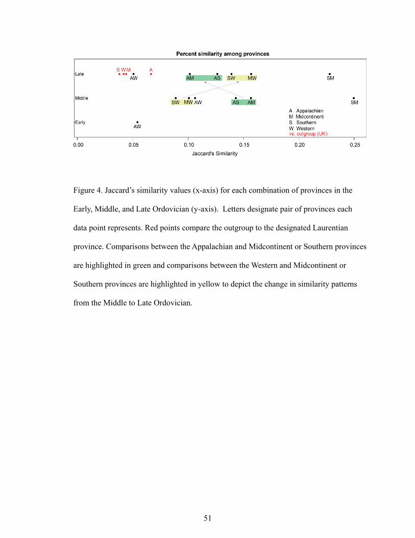
Figure 4. Jaccard’s similarity values (x-axis) for each combination of provinces in the
Early, Middle, and Late Ordovician (y-axis). Letters designate pair of provinces each
data point represents. Red points compare the outgroup to the designated Laurentian
province. Comparisons between the Appalachian and Midcontinent or Southern provinces
are highlighted in green and comparisons between the Western and Midcontinent or
Southern provinces are highlighted in yellow to depict the change in similarity patterns
from the Middle to Late Ordovician.
51

Fig
ure
5. J
acca
rd S
imil
arit
y (x
-axi
s) v
alue
s fo
r ea
ch p
airw
ise-
com
pari
son
amon
g co
llec
tion
s in
sub
regi
ons.
Wit
hin-
App
alac
hian
com
pari
sons
are
in g
reen
. App
alac
hian
vs.
Cin
cinn
ati c
ompa
riso
ns a
re in
dar
ker
oran
ge, A
ppal
achi
an v
s. N
ashv
ille
com
pari
sons
are
in
ligh
ter
oran
ge. N
umbe
rs c
orre
spon
d to
whi
ch A
ppal
achi
an s
ubre
gion
is in
volv
ed in
the
com
pari
son.
Gre
y ba
rs r
epre
sent
the
95%
conf
iden
ce in
terv
al. S
outh
to n
orth
dec
reas
e in
sim
ilar
ity
amon
g co
mpa
riso
ns b
etw
een
App
alac
hian
and
Sou
ther
n P
rovi
nce
coll
ecti
ons
is a
ppar
ent f
or b
oth
type
s of
dat
a.
52

Figure 6. Ordination of collections in the regional-scale study. Southern Province
collections (orange) exhibit lower NMDS1 scores than Appalachian (green) collections.
NMDS1 scores become more positive to the north within the Appalachian regions.
Collections from Nashville have lower NMDS2 scores than Cincinnati collections.
53

Figure 7. Taxon scores from the regional scale ordination. Orthorhynchula, gastropods,
and bivalves typical of sandier substrates and the northern Appalachian collections have
the most positive NMDS1 scores.
54

Fig
ure
8. J
acca
rd’s
sim
ilar
ity
(y-a
xis)
vs.
dis
tanc
e be
twee
n th
e ce
ntro
id o
f ea
ch s
et o
f co
llec
tion
s (x
-axi
s). G
rey
segm
ents
are
95%
conf
iden
ce in
terv
als.
Sim
ilar
ity
decr
ease
s w
ith
dist
ance
. Fit
is n
ot p
arti
cula
rly
stro
ng f
or a
ny o
f th
e re
gres
sion
mod
els.
A. c
onta
ins
the
enti
re d
ata
set,
colo
r co
ded
by c
ompa
riso
n, d
ashe
d li
ne is
the
fitt
ed m
odel
. B. C
inci
nnat
i/A
ppal
achi
an c
ompa
riso
ns. G
rey
dash
ed li
ne
show
s fi
t for
the
who
le d
ata
set,
blac
k da
shed
line
sho
ws
the
fit l
ine
for
Cin
cinn
ati/
App
alac
hian
col
lect
ions
onl
y. N
umbe
rs c
orre
spon
d
to w
hich
App
alac
hian
sub
regi
on th
e da
tum
rep
rese
nts.
C. N
ashv
ille
/App
alac
hian
com
pari
sons
.D. W
ithi
n-A
ppal
achi
an c
ompa
riso
ns.
55

Figure 9. A schematic representation of the proposed gradient in the Late Ordovician of
Laurentia (basemap from Blakey 2013)
56

Appendix 1. Paleobiology Database collection numbers used in this study, sorted by age and province.
Age: EarlyProvince: Appalachian 290 6971 6980 7105 42782 42793 42798 85184 88887 89489 89490 89491 89492 89501 89502 90082 90194 90195 98439 101293 119376 119377
Age:EarlyProvince: Midcontinent 101016
Age: EarlyProvince: SouthernN/A
Age: EarlyProvince: Western 429 11033 11034 11036 11039 11046 11047 11048 11050 11060 11063 11064 11072 56140 64502 66828 66832 66837 66841 66842 66843 66845 66847 66848 66849 66851 66852 66853 66854 66855 66856 66857 66858 66859 66860 66861 66864 69261 77844 77845 88805 88827 88838 88939 89013 103540 103784 103785 103786 103787 103788 103789 103790 103791 103792 103799 103800 103801 103803 103805 103806 103809 103810 103813 103814 103816 103817 103819 103820 103821 103822 103823 103824 103825 103826 103827 103829 103831 103888 103889 103891 103905 103906 103907 103908 103911 103912 103913 103916 103917 103918 103919 103920 104058 104059 104060 104061 104062 104063 104066 104067 104070 104071 104072 104073 104075 104076 104077 104079 104081 104082 104083 104084 104085 104086 104087 104089 104090 104091 104092 104094 104096 104097 104099 104100 104101 104102 104103 104104 104105 104106 104109 104110 104113 104115 104116 104118 104119 104121 104122 104123 104124 104126 104127 104128 104129 104130 104131 104132 104133 104134 104135 104137 104138 104141 104144 104145 104146 104147 104152 104153 104157 104158 104159 104160 104161 104162 104163 104164 104165 104167 104168 104169 104170 104171 104172 104173 104174 104175 104176 104177 104178 104180 104181 104183 104184 104185 104187 104188 104189 104190 104191 104262 104263 104264 104265 104266 104278 104279 104280 104281 104282 104283 104284 104285 104286 104287 104289 104290 104299 104301 104303 104304 104305 104306 104307
57

104308 104312 104314 104315 104360 104361 104363 104364 104433 104434 104436 104438 104439 104440 104441 104467 104468 104469 104470 104471 104472 104475 104476 104478 104558 104561 104563 104565 104568 104570 104571 104630 104631 104632 104633 104636 104638 104639 104640 104641 105090 105094 105776 105777 105779 105780 106370 106373 106374 106375 106387 106389 106390 106391 106392 106393 106394 106397 106398 106399 106420 106421 106422 106743 106745 106750 106751 106754 106755 106761 106763 106764 106765 106766 106770 106777 106778 106784 106788 106789 106790 106792 106794 106796 106799 106800 106801 106803 106806 106811 106818 106819 106822 106825 106834 106835 106836 106935 106936 106937 106939 106941 106942 106943 106946 106948 106949 106952 106954 106955 106957 106958 106960 106962 106964 143889
Age: MiddleProvince: Appalachian 319 329 6984 6989 6990 6991 6992 7093 7095 7096 7097
Age: MiddleProvince: Midcontinent 333 336 416 417 26174 26175 26188 26191
Age: MiddleProvince: Southern 1697 1698 1700 1706 1916 1922 1923 1925 1928 1940 1941 1944 1945 1946 1947 1955 1956 1957 1958 5327 5329 5333 5346 5351 5352 5355 5356 5357 5361 6707 6708 6709 85803 86054 86055 86056 86057 86058 86059 86081 86084 86087 86088 86089 86090 86091 86095 86096 86097 86101 86102 86103 86106 86124 86126 86128 86130 86133 86134 86135 86136 86137 86141 86142 86144 86145 86146 86191 86192 86193 86194 86195 86196 87734 87737 87739
Age: MiddleProvince: Western 296 301 305 310 311 318 425 13605 14229 25172 25173 25177 25857 25861 65131 65136 65141 65147
58

65151 80618 80619 102232 102233 102234 102236 102251 102252 102253 102255 102256 102258 102259 102261 102262 102263 102264 102265 102266 102267 102478 102479 102480 102485 103781 103909 103910 103914 103915 104268 104369 104370 104372 104373 104374 104375 104376 104378 104379 104380 104381 104383 104384 104386 104388 104389 104390 104391 104392 104393 104394 104395 104397 104398 104399 104400 104401 104402 104403 104404 104406 104408 104409 104410 104413 104417 104418 104423 104424 104426 104427 104429 104430 104431 104634 104653 104654 104655 104863 104870 104871 104873 104874 104875 104876 104877 104878 104879 104880 104881 104882 104883 104884 104885 104886 104887 104888 105612 105615 105635 105636 105641 105647 105648 105654
Age: LateProvince: Appalachian*Collections from Bretsky (1970: Table 3) begin with B. *Hyphenated collections are from the fieldwork of this study. 32398 32402 32456 32457 32458 32462 32465 32466 32467 B100 B101 B108 B110 B111 B112 B120 B123 B125 B126 B127 B128 B130 B131 B132 B133 B135 B136 B137 B138 B139 B140 B141 B142 B143 B144 B145 B147 B148 B149 B150 B151 B152 B153 B160 B161 B162 B163 B164 B166 B167 B168 B169 B170 B171 B172 B173 B174 B175 B177 B178 B179 B181 B182 B183 B184 B185 B186 B187 B188 B189 B190 B191 B192 B193 B194 B195 B196 B197 B199 B200 B201 B202 B203 B204 B205 B206 B32 B33 B37 B45 B47 B49 B60 B62 B63 B66 B68 B70 B71 B78 B81 B82 B84 B86 B87 B92 B93 B94 B95 B96 B97 B98 B99 RNG-3 CAT-3 CPM-3 STK-3 TH-3 CAT-1 TIP-1 CPM-2 NFM-1 STK-1 NAR-2 H16-2 AIR-1 ROY-3 CAT-2 H16-4 NFM-3 TIP-3 ROY-1 AL-3 NFM-2 RNG-4 RNG-1 H16-3 HAG-2 RNG-2 AIR-2 STK-2 HAG-1 ROY-2 TH-2 TH-1 NAR-1 TIP-2 CPM-1 HAG-3
59

Age: LateProvince: Midcontinent 356 357 396 421 6901 6902 6903 6904 6905 6906 6907 6908 6909 6910 6911 6913 13156 13200 22954 22956 22957 22961 26303 26304 55456 55457 55458 55459 55999
Age: LateProvince: Southern 350 354 361 374 375 382 398 399 1699 1710 1892 1893 1895 1918 1921 1927 1929 1930 1963 1972 1973 1974 1975 1976 1977 1978 1979 5323 5324 5325 5372 5373 5374 5392 5394 6900 34558 34559 34561 37833 48743 48749 48751 48752 48753 48754 48755 48756 48757 48758 48759 48765 48766 48767 48782 48783 48784 48785 48786 48787 48796 48797 48798 48799 48800 48802 48804 48807 48809 48810 48811 48812 48813 48818 48819 48820 48821 64166 64167 64169 64416 64417 64418 64419 64420 72427 72428 72429 72444 72445 72446 72447 72448 72449 72450 72454 72455 72456 72457 72458 72459 72460 72461 72462 72463 72464 72465 72466 72467 72468 72469 72470 72471 72522 72525 72528 72529 72530 72531 72532 72535 72536 72537 72538 72539 72540 72579 72580 72581 72582 72583 72584 72585 72586 72587 72588 72589 72590 72603 72604 72605 72606 72627 72628 72629 72630 72631 72632 72633 72634 72635 72636 72670 72671 72672 72673 72681 72682 72683 72684 72685 72686 72687 72688 72689 72690 72691 72692 72693 72694 72698 72699 72700 72701 72702 72703 72704 72705 72706 72707 72720 72722 72723 72724 72725 72737 72747 72748 72749 72750 72751 72752 72753 72754 72793 72794 72795 72796 72797 72798 72799 72800 72801 72802 72803 72812 72813 72814 72815 72816 72817 72818 72819 72820 72821 72822 72823 72824 72825 72826 72827 72829 72830 72831 72832 72841 72842 72844 72845 72846 72847 72848 72849 72850 72851 72863 72864 72865 72867 72868 72869 72888 72889 72924 72925
60

72936 72943 72944 72945 72946 72947 72948 72949 72950 72951 72952 72953 72964 72965 72966 72967 72984 72985 72986 72987 72988 72989 72990 73024 73025 73026 73027 73028 73029 73036 73037 73038 73039 73040 73042 73044 73045 73048 73049 73050 73051 73052 73083 73084 73085 73086 73103 73104 73105 73106 73115 73116 73117 73118 73119 73120 73121 73125 73127 73128 73129 73130 77144 85804 85805 85806 85810 85811 85812 85818 85820 85821 85822 85823 85824 85966 85974 85975 85976 85977 85979 85980 85990 85992 85993 85994 85995 85998 86004 86005 86008 86049 86050 86051 86052 86053 86060 86061 86062 86063 86064 86065 86066 86076 86077 86078 86079 86197 86198 86199 86200 86201 86202 86203 86204 86205 86206 86207 86208 86209 86210 86211 86212 86213 86214 86215 86216 86217 86218 86219 86220 86221 86222 86223 86224 86225 86226 86227 86228 86230 86231 86232 86233 86234 87813 87820 87821 87822 87825 87915 87932 87959 89538
Age: LateProvince: Western 10338 10442 10638 24124 24166 25319 25320 25321 25493 25506 25508 25514 25552 26070 26071 26921 26937 26938 26939 26940 26941 26942 26943 26944 26945 26946 26947 26948 26949 26950 26951 26952 26953 26954 26955 26956 26957 27246 27248 27251 27252 27253 27255 27256 27257 27258 27259 27280 27281 27283 27284 27286 27288 27291 27301 27302 27303 27305 27306 27307 27308 27309 27310 27426 27427 27428 27429 27430 27488 27489 27490 27494 28019 55455 55460 65153 65155 65235 80620 101902 101984 104326 104327 104329 104331 104332 104333 104522 109064 109065 109070 109071 113017
Age: LateProvince: United Kingdom (Outgroup)3370 45273 45274 45275 45276 45277 4527845279
61

Appendix 2. Southern Province collections used in the regional scale analysis (Patzkowsky and Holland 1999; Holland and Patzkowsky 2007)
Cincinnati Collections (Holland and Patzkowsky 2007)2S002, 2S003, 2S004, 2S005, 2S006, 2S007, 2S008, 2S009, 2S010, 2S011, 2S012, 2S013, 2S014, 2S015, 2S016, 2S017, 2S018, 2S019, 2S020, 2S021, 2S022, 2S023, 2S024, 2S025, 2S026, 2S027, 2S028, 2S029, 2S030, 2S031, 2S032, 2S033, 2S034, 2S035, 2S036, 2S037, 2S038, 2S039, 2S040, 2S041, 2S042, 2S043, 2S044, 2S045, 2S046, 2S047, 2S048, 2S049
Nashville Collections (Patzkowsky and Holland 1999)95PUW1, 95DF1, 95DF2, 95DF4, 95VVW12, 95VVW13, 95SCD8, 94HT2, 93VVW2, 95VVW13, 95SCD8, 94HT2, 93VVW2, 93SCD2, 95PU1, 95PUW10, 97GC6
62

Box bifoliateRNG-1 1 0 23 0 0 0 0RNG-2 1 3 27 0 0 0 0RNG-3 1 0 11 0 0 0 0RNG-4 1 0 0 0 0 0 0HAG-1 2 1 101 22 0 0 0HAG-2 2 0 22 0 0 0 0HAG-3 2 2 2 7 1 2 0STK-1 2 7 13 30 0 0 0STK-2 2 20 6 2 0 0 0STK-3 2 0 11 3 0 0 0TH-1 2 1 0 37 0 0 0TH-2 2 2 108 54 0 0 0TH-3 2 27 86 3 0 0 0TIP-1 2 1 11 22 0 0 0TIP-2 2 1 10 0 0 0 0TIP-3 2 2 4 2 0 0 0AIR-1 3 18 0 2 0 3 0AIR-2 3 0 0 0 0 0 0CAT-1 3 0 5 0 0 0 3CAT-2 3 13 0 0 3 1 0CAT-3 3 8 0 2 0 1 0NAR-1 3 9 0 5 0 0 0NAR-2 3 18 0 25 0 0 0CPM-1 4 9 0 0 0 0 0CPM-2 4 2 0 0 0 0 0CPM-3 4 0 0 0 0 0 0NFM-1 4 77 0 10 0 1 0NFM-2 4 19 0 4 0 1 0NFM-3 4 7 0 24 0 0 0AL-3 5 0 3 0 0 0 0H16-2 5 1 0 0 1 0 0H16-3 5 3 0 0 0 0 0H16-4 5 5 2 0 0 0 0ROY-1 5 4 0 0 0 0 0ROY-2 5 0 2 0 1 0 0ROY-3 5 0 0 0 0 0 0
Ambonychia Anazyga Bucanella Caritodens Cuffeyella
63

encrustingRNG-1 0 0 0 0 0 0 0RNG-2 1 0 1 0 0 0 0RNG-3 0 0 6 0 0 0 0RNG-4 0 0 0 0 0 0 0HAG-1 2 0 0 0 0 0 0HAG-2 0 0 0 0 0 0 0HAG-3 1 0 11 0 0 0 0STK-1 0 0 43 1 0 0 0STK-2 2 0 39 18 0 0 0STK-3 0 0 8 3 0 0 0TH-1 0 0 39 0 0 0 0TH-2 1 0 0 0 0 0 0TH-3 2 0 4 0 0 0 0TIP-1 1 0 32 0 0 0 0TIP-2 1 0 38 0 0 0 0TIP-3 0 0 2 0 0 0 0AIR-1 0 0 0 0 0 4 0AIR-2 1 0 0 2 0 51 0CAT-1 0 0 5 0 0 0 0CAT-2 0 0 0 0 0 26 0CAT-3 0 1 0 3 0 32 0NAR-1 0 0 0 1 0 0 0NAR-2 0 0 0 1 0 0 0CPM-1 0 0 0 4 0 0 0CPM-2 0 0 0 3 0 0 0CPM-3 0 0 0 3 0 0 0NFM-1 0 0 0 0 0 0 0NFM-2 1 0 0 2 0 0 0NFM-3 0 0 1 0 0 0 0AL-3 0 0 0 0 0 0 0H16-2 0 0 0 0 0 0 0H16-3 0 0 0 0 1 0 0H16-4 0 0 0 0 0 0 2ROY-1 0 0 0 0 0 8 0ROY-2 0 0 0 0 0 2 0ROY-3 0 0 0 1 0 6 0
eurypterid Hebertella Ischyrodonta Isotelus lingulid Liospira
64

RNG-1 0 0 0 0 0RNG-2 1 3 0 0 0RNG-3 0 0 3 0 0RNG-4 1 1 0 0 0HAG-1 0 0 0 0 0HAG-2 0 0 0 0 0HAG-3 2 0 0 0 0STK-1 0 0 0 0 0STK-2 0 5 0 0 5STK-3 0 3 0 0 0TH-1 0 0 0 0 0TH-2 0 0 0 0 0TH-3 0 1 0 0 0TIP-1 0 0 0 0 0TIP-2 0 0 0 0 0TIP-3 0 1 0 0 0AIR-1 3 3 1 19 0AIR-2 0 2 2 0 0CAT-1 0 0 0 0 0CAT-2 13 1 0 0 0CAT-3 49 2 0 3 0NAR-1 2 0 0 13 0NAR-2 1 1 0 33 0CPM-1 0 1 0 85 0CPM-2 0 1 0 33 0CPM-3 3 0 0 40 0NFM-1 0 4 2 66 0NFM-2 0 4 0 123 0NFM-3 0 0 0 53 0AL-3 1 0 0 1 0H16-2 2 2 0 0 0H16-3 1 1 2 0 0H16-4 55 0 7 8 0ROY-1 5 3 0 2 0ROY-2 6 0 0 2 0ROY-3 0 3 0 1 0
Lophospira Modiolopsis nautiloid Orthorhynchula Palaeonella
65

ramoseRNG-1 0 0 2 26 0RNG-2 0 6 0 26 0RNG-3 0 0 0 25 0RNG-4 0 0 0 4 0HAG-1 0 0 0 236 0HAG-2 0 0 0 0 0HAG-3 5 4 0 28 0STK-1 0 1 0 47 0STK-2 0 0 0 38 0STK-3 0 0 0 160 0TH-1 0 1 34 41 0TH-2 0 0 2 135 0TH-3 0 0 1 54 0TIP-1 0 0 0 100 0TIP-2 0 0 0 101 0TIP-3 3 0 0 31 0AIR-1 0 26 0 52 0AIR-2 0 23 0 10 0CAT-1 0 0 0 0 0CAT-2 0 38 0 0 0CAT-3 0 78 0 4 0NAR-1 0 6 0 3 2NAR-2 0 11 0 17 0CPM-1 0 0 0 0 0CPM-2 0 0 0 0 0CPM-3 0 0 0 0 0NFM-1 0 1 0 12 0NFM-2 0 2 0 11 0NFM-3 0 0 0 7 0AL-3 0 0 0 0 0H16-2 0 0 0 0 0H16-3 0 0 0 0 0H16-4 0 1 0 0 0ROY-1 0 25 0 0 0ROY-2 0 15 0 0 0ROY-3 0 18 1 0 0
Platystrophia Plectonotus Rafinesquina Sowerbyella
66

thin bifoliate thin ramoseRNG-1 17 0 0 0 0RNG-2 37 0 0 0 0RNG-3 12 0 0 0 0RNG-4 8 0 0 0 0HAG-1 0 0 0 0 0HAG-2 0 0 0 0 0HAG-3 0 8 6 1 0STK-1 0 0 0 0 0STK-2 0 0 0 0 0STK-3 4 5 0 0 0TH-1 0 0 0 2 0TH-2 0 0 0 4 0TH-3 0 0 6 2 0TIP-1 0 0 0 0 0TIP-2 0 0 0 0 0TIP-3 0 0 0 0 0AIR-1 0 26 0 0 0AIR-2 0 6 0 0 0CAT-1 106 0 0 0 0CAT-2 5 10 0 0 0CAT-3 0 10 0 0 1NAR-1 0 0 0 40 0NAR-2 0 5 0 3 0CPM-1 0 1 0 0 0CPM-2 0 0 0 0 0CPM-3 0 26 0 0 0NFM-1 0 0 0 0 0NFM-2 0 0 0 0 0NFM-3 0 0 2 0 0AL-3 0 0 0 0 0H16-2 0 0 0 0 0H16-3 0 1 0 0 0H16-4 0 0 0 0 0ROY-1 0 5 0 0 0ROY-2 0 0 0 0 0ROY-3 0 0 0 0 0
Strophomena Tancrediopsis Treptostome
67

trilobiteRNG-1 1 5RNG-2 0 0RNG-3 3 0RNG-4 0 35HAG-1 0 0HAG-2 0 21HAG-3 0 7STK-1 0 9STK-2 0 16STK-3 0 3TH-1 0 0TH-2 0 0TH-3 0 0TIP-1 0 8TIP-2 0 8TIP-3 0 42AIR-1 0 7AIR-2 0 0CAT-1 0 0CAT-2 0 0CAT-3 0 0NAR-1 0 22NAR-2 0 7CPM-1 0 4CPM-2 0 12CPM-3 0 5NFM-1 0 2NFM-2 0 3NFM-3 0 3AL-3 0 0H16-2 0 0H16-3 0 0H16-4 0 0ROY-1 0 0ROY-2 0 0ROY-3 0 0
Zygospira
68

Appendix 4. Locality information for Appalachian collections
Region 1Ringgold (RNG): Large (multistory) road cut on south side of Georgia Route 75, east of
Catoosa. It is not accessible from the highway, must park behind the carpet factories and hike back. 34.908° N, 85.105°W.
Region 2Hagan (HAG): Railroad cut on the east side of the railroad tracks at Hagan, Virginia.
36.702°N, 83.289°W.Stickleyville (STK): Road cut on south side of Virginia Route 58, .2 miles west of
junction between Route 58 and Route 726. 36.711°N, 82.877°W.Thorn Hill (TH): Road cut on the south side of Tennessee Route 25, just west of the
intersection between Old Mountain Road and Route 25. 36.35232°N, 83.400°W.Tiprell Road (TIP): Railroad cut at the foot of a hill below Tiprell Road, just beyond (less
than .1 miles) where Tiprell Road forks and turns up that same hill, south of Cumberland Gap, Tennessee. 36.567°N, 83.676°W.
Region 3Airport Road (AIR): Roadcut on Route 606, just below junction with Route 703 (Airport
Road) on Warm Springs Mountain. 37.876°N, 79.888°W.Catawba (CAT): Roadcut on the south side of Virginia Route 311, just uphill from the
guardrail, near Catawba, Virginia. 37.380°N, 80.090°W.Narrows (NAR): Roadcut on the east side of Virginia Route 460, northbound, on the east
side of the river near Narrows, Virginia . 37.352°N, 80.809°W.
Region 4North Fork Mountain (NFM): Roadcut on south side of 33-W, western side of North Fork
Mountain, West Virginia, about .6 miles past the antenna at the top of the mountain, heading west. 38.708°N, 79.411°W.
Coopers Mountain (CPM): Roadcut on the east side of Virginia Route 732 (Coopers Mountain Road) approximately 1.4 miles south of Route 33. 38.480°N, 79.026°W.
Region 5Allensville (AL): Roadcut on Allensville Mountain Road, .65 miles after (north of) the
intersection with Barr Road with near Allensville, Pennsylvania. 40.557°N, 77.821°W.
Highway 16 (H16): Roadcut on Highway 16 on Tuscarora Mountain, SE of McConnellsburg, Pennsylvania. 39.905°N, 77.966°W.
Loysburg (ROY): Roadcut on the north side of Pennsylvania Route 36 (Woodbury Pike), less than .1 miles east of junction with Town Hill Road, near Loysburg, Pennsylvania. 40.160°N, 78.373°W.
69

Appendix 5.
Continent-Scale SimilarityAge Provinces Jaccard's SimilarityEarly Appalachian Midcontinent N/A
Appalachian Southern N/AAppalachian Western 0.055Midcontinent Southern N/AMidcontinent Western 0.009Southern Western N/A
Middle Appalachian Midcontinent 0.157Appalachian Southern 0.144Appalachian Western 0.107Midcontinent Southern 0.250Midcontinent Western 0.101Southern Western 0.089
Late Appalachian Midcontinent 0.102Appalachian Southern 0.127Appalachian Western 0.051Midcontinent Southern 0.228Midcontinent Western 0.158Southern Western 0.140Appalachian U.K. 0.067Midcontinent U.K. 0.044Southern U.K. 0.038Western U.K. 0.042
70

Regional Scale SimilarityRelative Abundance
Subregions Distance (km)C N 0.139 0.13 0.149 3101 2 0.256 0.218 0.297 2501 3 0.066 0.036 0.118 5201 4 0.094 0.047 0.177 6701 5 0.041 0.021 0.078 8602 3 0.098 0.073 0.13 2902 4 0.116 0.087 0.154 4302 5 0.058 0.042 0.081 6103 4 0.071 0.039 0.126 1503 5 0.066 0.04 0.107 3504 5 0.119 0.093 0.151 2101 N 0.051 0.031 0.082 1802 N 0.047 0.034 0.065 3203 N 0.016 0.01 0.026 6104 N 0.050 0.032 0.077 7305 N 0.010 0.006 0.016 9001 C 0.211 0.203 0.219 3602 C 0.208 0.199 0.217 2103 C 0.146 0.136 0.157 3904 C 0.146 0.136 0.157 4505 C 0.075 0.066 0.085 610
Jaccard's Similarity
Lower Confidence Limit
Upper Confidence Limit
71
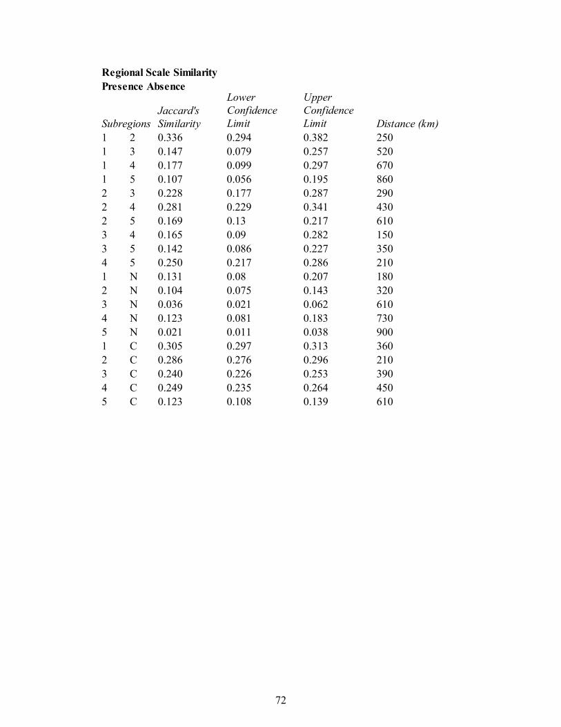
Regional Scale SimilarityPresence Absence
Subregions Distance (km)1 2 0.336 0.294 0.382 2501 3 0.147 0.079 0.257 5201 4 0.177 0.099 0.297 6701 5 0.107 0.056 0.195 8602 3 0.228 0.177 0.287 2902 4 0.281 0.229 0.341 4302 5 0.169 0.13 0.217 6103 4 0.165 0.09 0.282 1503 5 0.142 0.086 0.227 3504 5 0.250 0.217 0.286 2101 N 0.131 0.08 0.207 1802 N 0.104 0.075 0.143 3203 N 0.036 0.021 0.062 6104 N 0.123 0.081 0.183 7305 N 0.021 0.011 0.038 9001 C 0.305 0.297 0.313 3602 C 0.286 0.276 0.296 2103 C 0.240 0.226 0.253 3904 C 0.249 0.235 0.264 4505 C 0.123 0.108 0.139 610
Jaccard's Similarity
Lower Confidence Limit
Upper Confidence Limit
72

##Appendix 6#Continental Scale then regional scale
#Load Librarieslibrary(vegan)library(boot)library(car)#Read in dataLaurentia<-read.csv("Ord_occs.csv",header=TRUE,sep=",",as.is=TRUE)provremod<-read.csv("provremod.csv",header=TRUE,sep=",",as.is=TRUE)col_age<-read.csv("col_age.csv",header=TRUE,sep=",",as.is=TRUE)outgroup<-read.csv("UK-culled.csv",header=T,sep=",")bretsky<-read.csv("BretskyAppCollCull.csv",header=TRUE,sep=",",row.names=1)app2013<-read.csv("Appalachian_2013.csv",header=TRUE,sep=",",row.names=1)AbundanceMatrix<-read.csv("AbundanceMatrix.csv",header=TRUE,sep=",",row.names=1)paradist<-read.csv("paradist.csv")
###############CONTINENTAL SCALE#################################prep data
#check rows, should be 0which(Laurentia$collection_no!=provremod$collection)
#put province data in occurrence tableLaurentia<-cbind(Laurentia,provremod)
#Clean up the data#Nix the Lingula (but not Lingulasma)Laurentia$occurrence.genus_name<-gsub("Lingula$","Lingulid",Laurentia$occurrence.genus_name)
#Nix the blank environmentsLaurentia<-Laurentia[which(Laurentia$environment!=""),]
#Oust DalveLaurentia<-Laurentia[which(Laurentia$collection_no!=389&Laurentia$collection_no!=391&Laurentia$collection_no!=394),]
#Nix SchizambonLaurentia<-Laurentia[which(Laurentia$occurrence.genus_name!="Schizambon"),]
#check collections still match (should = 0)which(Laurentia$collection_no != col_age$collection_no)
#Put ages in now, this table was built off the culled Laurentia
73

Laurentia<-cbind(Laurentia,col_age)
#Correct MisspellingsLaurentia$occurrence.genus_name<-gsub("Apheorthis","Apheoorthis",Laurentia$occurrence.genus_name)Laurentia$occurrence.genus_name<-gsub("Cerurinella","Ceraurinella",Laurentia$occurrence.genus_name)Laurentia$occurrence.genus_name<-gsub("Cymatonata","Cymatonota",Laurentia$occurrence.genus_name)Laurentia$occurrence.genus_name<-gsub("Drepanodos","Drepanodus",Laurentia$occurrence.genus_name)Laurentia$occurrence.genus_name<-gsub("Heterotrpya","Heterotrypa",Laurentia$occurrence.genus_name)Laurentia$occurrence.genus_name<-gsub("Hormotelus","Homotelus",Laurentia$occurrence.genus_name)Laurentia$occurrence.genus_name<-gsub("Missiquoia","Missisquoia",Laurentia$occurrence.genus_name)Laurentia$occurrence.genus_name<-gsub("Paterulus","Paterula",Laurentia$occurrence.genus_name)Laurentia$occurrence.genus_name<-gsub("Pauposira","Paupospira",Laurentia$occurrence.genus_name)Laurentia$occurrence.genus_name<-gsub("Pionodema","Pianodema",Laurentia$occurrence.genus_name)
#Nix CameratesLaurentia<-Laurentia[which(Laurentia$occurrence.genus_name!="Camerate"),]
#Nix SkolithosLaurentia<-Laurentia[which(Laurentia$occurrence.genus_name!="Skolithos"),]
#Add outgroup Laur<-Laurentia[,c(1,3,5,11,12,17,21,27,29)]Out<-outgroup[,c(1,4,6,17,18,23,30)]Prov<-replicate(length(rownames(Out)),5)Age<-replicate(length(rownames(Out)),3)Out<-cbind(Out,Prov,Age)
occdata<-rbind(Laur,Out)
#######
#Generate the Occurrence Matrix#make sure province and age column are called "Prov" and "Age"
#If you are trying to add data to the occurrence matrix you need to put your collections in here
addnames<-sort(unique(c(names(bretsky),names(app2013))))addrows<-c(rownames(bretsky),rownames(app2013))
74

GenerateOccurrenceMatrix<-function(pbdbdata,addins){if (addins=="TRUE"){
UniqueGenera<-sort(unique(c(pbdbdata$occurrence.genus_name,addnames)))
UniqueCollections<-unique(c(pbdbdata$collection_no,addrows))
}else {UniqueGenera<-sort(unique(pbdbdata$occurrence.genus_name))UniqueCollections<-unique(pbdbdata$collection_no)}
Occurrences <- matrix(data=0, nrow=length(UniqueCollections), ncol=length(UniqueGenera)+2, dimnames=list(UniqueCollections,c(UniqueGenera,"Province","Age")))
for (i in 1:nrow(pbdbdata)){ CollectionNumber <-
which(UniqueCollections==pbdbdata$collection_no[i])GenusNumber <-
which(UniqueGenera==pbdbdata$occurrence.genus_name[i]) Occurrences[CollectionNumber,GenusNumber] <-1Occurrences[CollectionNumber,length(UniqueGenera)+1]<-
as.numeric(pbdbdata$Prov[i])Occurrences[CollectionNumber,length(UniqueGenera)+2]<-
as.numeric(pbdbdata$Age[i])
}Occurrences<-as.data.frame(Occurrences)Occurrences
}OccurrenceMatrix<-GenerateOccurrenceMatrix(occdata,TRUE)
#Make sure nothing got weird (should be 0)which(rownames(OccurrenceMatrix) != unique(c(occdata$collection_no,addrows)))
#Fill in added rowsOccurrenceMatrix[which(rownames(OccurrenceMatrix)%in%addrows),names(OccurrenceMatrix)=="Province"]<-1OccurrenceMatrix[which(rownames(OccurrenceMatrix)%in%addrows),names(OccurrenceMatrix)=="Age"]<-3
for (i in 1:nrow (bretsky)){colnumber<-which(rownames(bretsky)
[i]==rownames(OccurrenceMatrix))filllist<-names(bretsky)[which(bretsky[i,]>0)]GenusNumbers<-which(names(OccurrenceMatrix)%in
%filllist)OccurrenceMatrix[colnumber,GenusNumbers]<-1
}
75

for (i in 1:nrow (app2013)){colnumber<-which(rownames(app2013)
[i]==rownames(OccurrenceMatrix))filllist<-names(app2013)[which(app2013[i,]>0)]GenusNumbers<-which(names(OccurrenceMatrix)%in
%filllist)OccurrenceMatrix[colnumber,GenusNumbers]<-1
}
#Eliminate morpho-bryozoan (unique to added app collections) and "nautiloid"OccurrenceMatrix<-OccurrenceMatrix[,names(OccurrenceMatrix)!="nautiloid"]bryos<-grep("Bryozoan.",names(OccurrenceMatrix))OccurrenceMatrix<-OccurrenceMatrix[,names(OccurrenceMatrix)[-bryos]]
#Eliminate singleton collectionsOccurrenceMatrix<-OccurrenceMatrix[which(rowSums(OccurrenceMatrix[,c(names(OccurrenceMatrix)!="Province" & names(OccurrenceMatrix)!="Age")])>1),]
#################################################################
####Aggregate, continent scale, Early/Middle/Late
P11<-OccurrenceMatrix[which(OccurrenceMatrix$Province==1 & OccurrenceMatrix$Age==1),]
P11<-rbind(P11,colSums(P11))AggP11<-P11[nrow(P11),]AggP11$Province<-1AggP11$Age<-1
P21<-OccurrenceMatrix[which(OccurrenceMatrix$Province==2 & OccurrenceMatrix$Age==1),]
P21<-rbind(P21,colSums(P21))AggP21<-P21[nrow(P21),]AggP21$Province<-2AggP21$Age<-1
if(length(which(OccurrenceMatrix$Province==3 & OccurrenceMatrix$Age==1))==0)
{AggP31<-AggP21AggP31[,which(names(AggP31)=="Province")]<-3AggP31[1,1:(length(names(AggP31))-2)]<-
replicate(length(names(AggP31))-2,0)}
if(length(which(OccurrenceMatrix$Province==3 & OccurrenceMatrix$Age==1))>0){
P31<-OccurrenceMatrix[which(OccurrenceMatrix$Province==3 & OccurrenceMatrix$Age==1),]
P31<-rbind(P31,colSums(P31))
76

AggP31<-P31[nrow(P31),]AggP31$Province<-3AggP31$Age<-1}
P41<-OccurrenceMatrix[which(OccurrenceMatrix$Province==4 & OccurrenceMatrix$Age==1),]
P41<-rbind(P41,colSums(P41))AggP41<-P41[nrow(P41),]AggP41$Province<-4AggP41$Age<-1
P12<-OccurrenceMatrix[which(OccurrenceMatrix$Province==1 & OccurrenceMatrix$Age==2),]
P12<-rbind(P12,colSums(P12))AggP12<-P12[nrow(P12),]AggP12$Province<-1AggP12$Age<-2
P22<-OccurrenceMatrix[which(OccurrenceMatrix$Province==2 & OccurrenceMatrix$Age==2),]
P22<-rbind(P22,colSums(P22))AggP22<-P22[nrow(P22),]AggP22$Province<-2AggP22$Age<-2
P32<-OccurrenceMatrix[which(OccurrenceMatrix$Province==3 & OccurrenceMatrix$Age==2),]
P32<-rbind(P32,colSums(P32))AggP32<-P32[nrow(P32),]AggP32$Province<-3AggP32$Age<-2
P42<-OccurrenceMatrix[which(OccurrenceMatrix$Province==4 & OccurrenceMatrix$Age==2),]
P42<-rbind(P42,colSums(P42))AggP42<-P42[nrow(P42),]AggP42$Province<-4AggP42$Age<-2
P13<-OccurrenceMatrix[which(OccurrenceMatrix$Province==1 & OccurrenceMatrix$Age==3),]
P13<-rbind(P13,colSums(P13))AggP13<-P13[nrow(P13),]AggP13$Province<-1AggP13$Age<-3
P23<-OccurrenceMatrix[which(OccurrenceMatrix$Province==2 & OccurrenceMatrix$Age==3),]
P23<-rbind(P23,colSums(P23))AggP23<-P23[nrow(P23),]AggP23$Province<-2
77

AggP23$Age<-3
P33<-OccurrenceMatrix[which(OccurrenceMatrix$Province==3 & OccurrenceMatrix$Age==3),]
P33<-rbind(P33,colSums(P33))AggP33<-P33[nrow(P33),]AggP33$Province<-3AggP33$Age<-3
P43<-OccurrenceMatrix[which(OccurrenceMatrix$Province==4 & OccurrenceMatrix$Age==3),]
P43<-rbind(P43,colSums(P43))AggP43<-P43[nrow(P43),]AggP43$Province<-4AggP43$Age<-3
P53<-OccurrenceMatrix[which(OccurrenceMatrix$Province==5 & OccurrenceMatrix$Age==3),]
P53<-rbind(P53,colSums(P53))AggP53<-P53[nrow(P53),]AggP53$Province<-5AggP53$Age<-3
Aggregates<-rbind(AggP11,AggP21,AggP31,AggP41,AggP12,AggP22,AggP32,AggP42,AggP13,AggP23,AggP33,AggP43,AggP53)rownames(Aggregates)<-c(11,21,31,41,12,22,32,42,13,23,33,43,53)
interprovincesimilarityAgg<-function(ProvinceAn,ProvinceBn,Agen){
provinceageA<-Aggregates[Aggregates$Province==ProvinceAn & Aggregates$Age==Agen,colnames(Aggregates)!="Province"&colnames(Aggregates)!="Age"]
provinceageB<-Aggregates[Aggregates$Province==ProvinceBn & Aggregates$Age==Agen, colnames(Aggregates)!="Province" & colnames(Aggregates)!="Age"]
provinceage<-rbind(provinceageA,provinceageB)
similarity<-1-vegdist(provinceage, method="jaccard", binary=TRUE)
similarity}
#Aggregate Table
AggregateTable<-as.data.frame(matrix(data=9,nrow=22,ncol=4,dimnames=list(1:22,c("ProvinceA","ProvinceB","Age","similarity"))))
row <- 1
78

for (Age in 1:3){for (ProvinceA in 1:3){
for (ProvinceB in (ProvinceA+1):4){
if (ProvinceA==3 & Age==1|ProvinceB==3 & Age==1){ #no data
ips <- 9} else {
ips<-interprovincesimilarityAgg(ProvinceA,ProvinceB,Age)
}
#fill in rowAggregateTable[row,1] <- ProvinceAAggregateTable[row,2] <- ProvinceBAggregateTable[row,3] <- AgeAggregateTable[row,4] <- ips
# increment row number row <- row+1
}}
}row<-19for (ProvinceA in 1:4){
ProvinceB<-5Age<-3ips<-
interprovincesimilarityAgg(ProvinceA,ProvinceB,Age)
AggregateTable[row,1] <- ProvinceAAggregateTable[row,2] <- ProvinceBAggregateTable[row,3] <- AgeAggregateTable[row,4] <- ips
# increment row number row <- row+1}
AggregateTablewrite.csv(AggregateTable,"AggregateSimilarity.csv")
###PLOTplotagr<-AggregateTable[AggregateTable$similarity<9,]
stripchart(plotagr$similarity~plotagr$Age, xlim=c(0,max(plotagr$similarity)+.01), ylim=c(.5,3.5), xlab="Jaccard's Similarity",ylab="Age",las=1, pch=16, col="white", main="Aggregated Similarity")points(plotagr$similarity[plotagr$ProvinceB==5],
79

plotagr$Age[plotagr$ProvinceB==5], pch=16, col="firebrick2")points(plotagr$similarity[plotagr$ProvinceB!=5], plotagr$Age[plotagr$ProvinceB!=5], pch=16, col="black")points(plotagr$similarity[plotagr$Age==1&(plotagr$ProvinceA==2|plotagr$ProvinceB==2)],plotagr$Age[plotagr$Age==1&(plotagr$ProvinceA==2|plotagr$ProvinceB==2)],pch=16,col="white")
labelsage23<-c("AM","AS","AW","MS","MW","SW","AM","AS","AW","MS","MW","SW")simsage23<-plotagr$similarity[plotagr$ProvinceB!=5&plotagr$Age!=1]agesage23<-plotagr$Age[plotagr$ProvinceB!=5&plotagr$Age!=1]-.15text(c(simsage23),c(agesage23),col="black",cex=.8,label=c(labelsage23))
labelsage1<-c("AW")simsage1<-plotagr$similarity[plotagr$Age==1&plotagr$ProvinceA==1&plotagr$ProvinceB==4]agesage1<-plotagr$Age[plotagr$Age==1&plotagr$ProvinceA==1&plotagr$ProvinceB==4]-.15text(c(simsage1),c(agesage1),col="black",cex=.8,label=c(labelsage1))
labelsoutgroup<-c("A","M","S","W")simsoutgroup<-plotagr$similarity[plotagr$ProvinceB==5]agesoutgroup<-plotagr$Age[plotagr$ProvinceB==5]+.15text(c(simsoutgroup),c(agesoutgroup),col="fire brick 1",cex=.8,label=c(labelsoutgroup))
text(.2,1.4,col="black",cex=.8,label="A Appalachian")text(.2,1.2,col="black",cex=.8,label="M Midcontinent")text(.2,1.0,col="black",cex=.8,label="S Southern")text(.2,.8,col="black",cex=.8,label="W Western")text(.2,.6,col="fire brick 2",cex=.8,label=" outgroup (UK)")
###############################################Ranked ListsAbundanceList13<-sort(P13[nrow(P13),],decreasing=TRUE)AbundanceList23<-sort(P23[nrow(P23),],decreasing=TRUE)AbundanceList33<-sort(P33[nrow(P33),],decreasing=TRUE)AbundanceList43<-sort(P43[nrow(P43),],decreasing=TRUE)AbundanceList53<-sort(P53[nrow(P53),],decreasing=TRUE)List13<-AbundanceList13[,AbundanceList13>0]List23<-AbundanceList23[,AbundanceList23>0]List33<-AbundanceList33[,AbundanceList33>0]List43<-AbundanceList43[,AbundanceList43>0]List53<-AbundanceList53[,AbundanceList53>0]
sum13<-sum(List13[,names(List13)!="Province"&names(List13)!
80

="Age"])p13<-List13[,names(List13)!="Province"&names(List13)!="Age"]/sum13sum23<-sum(List23[,names(List23)!="Province"&names(List23)!="Age"])p23<-List23[,names(List23)!="Province"&names(List23)!="Age"]/sum23sum33<-sum(List33[,names(List33)!="Province"&names(List33)!="Age"])p33<-List33[,names(List33)!="Province"&names(List33)!="Age"]/sum33sum43<-sum(List43[,names(List43)!="Province"&names(List43)!="Age"])p43<-List43[,names(List43)!="Province"&names(List43)!="Age"]/sum43sum53<-sum(List53[,names(List53)!="Province"&names(List53)!="Age"])p53<-List53[,names(List53)!="Province"&names(List53)!="Age"]/sum53write.csv(p13,"abundancelistAL.csv")write.csv(p23,"abundancelistML.csv")write.csv(p33,"abundancelistSL.csv")write.csv(p43,"abundancelistWL.csv")write.csv(p53,"abundancelistUL.csv")
AbundanceList12<-sort(P12[nrow(P12),],decreasing=TRUE)AbundanceList22<-sort(P22[nrow(P22),],decreasing=TRUE)AbundanceList32<-sort(P32[nrow(P32),],decreasing=TRUE)AbundanceList42<-sort(P42[nrow(P42),],decreasing=TRUE)List12<-AbundanceList12[,AbundanceList12>0]List22<-AbundanceList22[,AbundanceList22>0]List32<-AbundanceList32[,AbundanceList32>0]List42<-AbundanceList42[,AbundanceList42>0]
sum12<-sum(List12[,names(List12)!="Province"&names(List12)!="Age"])p12<-List12[,names(List12)!="Province"&names(List12)!="Age"]/sum12sum22<-sum(List22[,names(List22)!="Province"&names(List22)!="Age"])p22<-List22[,names(List22)!="Province"&names(List22)!="Age"]/sum22sum32<-sum(List32[,names(List32)!="Province"&names(List32)!="Age"])p32<-List32[,names(List32)!="Province"&names(List32)!="Age"]/sum32sum42<-sum(List42[,names(List42)!="Province"&names(List42)!="Age"])p42<-List42[,names(List42)!="Province"&names(List42)!="Age"]/sum42
write.csv(p12,"abundancelistAM.csv")
81

write.csv(p22,"abundancelistMM.csv")write.csv(p32,"abundancelistSM.csv")write.csv(p42,"abundancelistWM.csv")
AbundanceList11<-sort(P11[nrow(P11),],decreasing=TRUE)AbundanceList21<-sort(P21[nrow(P21),],decreasing=TRUE)AbundanceList31<-sort(P31[nrow(P31),],decreasing=TRUE)AbundanceList41<-sort(P41[nrow(P41),],decreasing=TRUE)List11<-AbundanceList11[,AbundanceList11>0]List21<-AbundanceList21[,AbundanceList21>0]List31<-AbundanceList31[,AbundanceList31>0]List41<-AbundanceList41[,AbundanceList41>0]
sum11<-sum(List11[,names(List11)!="Province"&names(List11)!="Age"])p11<-List11[,names(List11)!="Province"&names(List11)!="Age"]/sum11sum21<-sum(List21[,names(List21)!="Province"&names(List21)!="Age"])p21<-List21[,names(List21)!="Province"&names(List21)!="Age"]/sum21sum31<-sum(List31[,names(List31)!="Province"&names(List31)!="Age"])p31<-List31[,names(List31)!="Province"&names(List31)!="Age"]/sum31sum41<-sum(List41[,names(List41)!="Province"&names(List41)!="Age"])p41<-List41[,names(List41)!="Province"&names(List41)!="Age"]/sum41
write.csv(p11,"abundancelistAE.csv")write.csv(p21,"abundancelistME.csv")write.csv(p31,"abundancelistSE.csv")write.csv(p41,"abundancelistWE.csv")
##############REGIONAL SCALE##########################Set up Data
RAmatrix1<-decostand(AbundanceMatrix[,names(AbundanceMatrix)!="Box"],"total")#Convert abundance matrix to relative abundanceBox<-AbundanceMatrix$BoxRAmatrix<-cbind(RAmatrix1,Box)
#########Abundance lists: Most abundant taxa in each box########
#Make a table of the sums of each genera in a box, divided by the number of individuals, this is basically relative abundance of the aggregate collections of each box. At the end this will spit out a list of the most abundant taxa in each collection
AggBoxTable<-
82

as.data.frame(matrix(data=9,nrow=7,ncol=length(names(AbundanceMatrix)), dimnames=list(1:7,c(names(AbundanceMatrix)))))for (i in 1:7){
Box<-AbundanceMatrix[which(AbundanceMatrix$Box==i),]Box<-rbind(Box,colSums(Box))aggBox<-Box[nrow(Box),]aggBox$Box<-iAggBoxTable[i,]<-aggBox}
#Convert this to relative abundanceAggBoxTableBox<-AggBoxTable$BoxAggBoxTable<-AggBoxTable[,names(AggBoxTable)!="Box"]RAagg<-decostand(AggBoxTable,"total")Boxes<-c(1:7)RAaggbox<-cbind(RAagg,Boxes)names(RAaggbox)[which(names(RAaggbox)=="Boxes")]<-"Box"
AbundanceListBox1<-round(sort(RAaggbox[RAaggbox$Box==1,],decreasing=TRUE),digits=2)AbundanceListBox2<-round(sort(RAaggbox[RAaggbox$Box==2,],decreasing=TRUE),digits=2)AbundanceListBox3<-round(sort(RAaggbox[RAaggbox$Box==3,],decreasing=TRUE),digits=2)AbundanceListBox4<-round(sort(RAaggbox[RAaggbox$Box==4,],decreasing=TRUE),digits=2)AbundanceListBox5<-round(sort(RAaggbox[RAaggbox$Box==5,],decreasing=TRUE),digits=2)AbundanceListBox6<-round(sort(RAaggbox[RAaggbox$Box==6,],decreasing=TRUE),digits=2)AbundanceListBox7<-round(sort(RAaggbox[RAaggbox$Box==7,],decreasing=TRUE),digits=2)(ListBox1<-AbundanceListBox1[,AbundanceListBox1>0])(ListBox2<-AbundanceListBox2[,AbundanceListBox2>0])(ListBox3<-AbundanceListBox3[,AbundanceListBox3>0])(ListBox4<-AbundanceListBox4[,AbundanceListBox4>0])(ListBox5<-AbundanceListBox5[,AbundanceListBox5>0])#Nashville(ListBoxN<-AbundanceListBox6[,AbundanceListBox6>0])#Cinci(ListBoxC<-AbundanceListBox7[,AbundanceListBox7>0])
######Similarity######
#Combines collections from the two called regions, calculates Jaccard's similarity #binary=1 for PA, binary=0 for RA
betweenBoxsimilarity<-function(BoxnA,BoxnB,binary){
boxA<-RAmatrix[RAmatrix$Box==BoxnA,colnames(RAmatrix)!
83

="Box"]boxB<-RAmatrix[RAmatrix$Box==BoxnB,colnames(RAmatrix)!
="Box"]twoboxes<-rbind(boxA,boxB)
if (binary=="FALSE"|binary==0){similarity<-1-vegdist(twoboxes, method="jaccard",
binary=FALSE)} else{similarity<-1-vegdist(twoboxes, method="jaccard",
binary=TRUE)}logitsim<-car::logit(similarity,adjust=.0001)ttest<-t.test(logitsim)sd<-sd(logitsim)
results<-c(ttest,sd) names(results)[10]<-"sd"
intresults<-c(ttest,sd)names(intresults)[10]<-"sd"results<-
c(inv.logit(intresults$estimate),inv.logit(intresults$conf.int[1]),inv.logit(intresults$conf.int[2]),inv.logit(intresults$sd))
names(results)<-c("estimate","LCL","UCL","sd")results
}
#Fill table:PA
PAbetweenBoxtable<-as.data.frame(matrix(data=9,nrow=21, ncol=6, dimnames=list(1:21, c("BoxA","BoxB","mean","LCL","UCL","sd"))))
row<-1
for (BoxA in 1:6) {for (BoxB in (BoxA+1):7){
bBs<-betweenBoxsimilarity(BoxA,BoxB,1)PAbetweenBoxtable[row,1]<-BoxAPAbetweenBoxtable[row,2]<-BoxBPAbetweenBoxtable[row,3]<-bBs[1]PAbetweenBoxtable[row,4]<-bBs[2]PAbetweenBoxtable[row,5]<-bBs[3]PAbetweenBoxtable[row,6]<-bBs[4]
#increment row counterrow<-row+1}
}
write.csv(PAbetweenBoxtable,"PAbetweenBoxtable.csv")(PAbetweenBoxtableRound<-round(PAbetweenBoxtable,3))
84

#Fill table:RARAbetweenBoxtable<-as.data.frame(matrix(data=9,nrow=21, ncol=6, dimnames=list(1:21, c("BoxA","BoxB","mean","LCL","UCL","sd"))))
row<-1
for (BoxA in 1:6) {for (BoxB in (BoxA+1):7){
bBs<-betweenBoxsimilarity(BoxA,BoxB,0)RAbetweenBoxtable[row,1]<-BoxARAbetweenBoxtable[row,2]<-BoxBRAbetweenBoxtable[row,3]<-bBs[1]RAbetweenBoxtable[row,4]<-bBs[2]RAbetweenBoxtable[row,5]<-bBs[3]RAbetweenBoxtable[row,6]<-bBs[4]
#increment row counterrow<-row+1}
}
write.csv(RAbetweenBoxtable,"RAbetweenBoxtable.csv")(RAbetweenBoxtableRound<-round(RAbetweenBoxtable,3))
####Plots
#Within-Box PA#windows()plot(rownames(PAwithinBoxtable)~PAwithinBoxtable$mean,type="n",las=1,main="Within-Box P/A",ylab="Box",xlab="Jaccard Similarity",xlim=c(0,max(PAwithinBoxtable$UCL)+.05))#Add confidence intervals, r is simply a row counterfor (r in 1:nrow(PAwithinBoxtable)){
segments(PAwithinBoxtable[r,2],r,PAwithinBoxtable[r,3],r,col="grey")}points(PAwithinBoxtable$mean[1:5],rownames(PAwithinBoxtable)[1:5],pch=16,col="steel blue 2")points(PAwithinBoxtable$mean[6],rownames(PAwithinBoxtable)[6],pch=16,col="orchid3")points(PAwithinBoxtable$mean[7],rownames(PAwithinBoxtable)[7],pch=16,col="orchid4")text(.12,6,col="orchid3",cex=.8,label="Nashville")text(.25,7,col="orchid4",cex=.8,label="Cincinnati")
#Within-Box: RA#windows()plot(rownames(RAwithinBoxtable)~RAwithinBoxtable$mean,type="n",las=1,main="Within-Box RA",ylab="Box",xlab="Jaccard
85

Similarity",xlim=c(0,max(RAwithinBoxtable$UCL)+.05))#Add confidence intervals, r is simply a row counterfor (r in 1:nrow(RAwithinBoxtable)){
segments(RAwithinBoxtable[r,2],r,RAwithinBoxtable[r,3],r,col="grey")}points(RAwithinBoxtable$mean[1:5],rownames(RAwithinBoxtable)[1:5],pch=16,col="steel blue 2")points(RAwithinBoxtable$mean[6],rownames(RAwithinBoxtable)[6],pch=16,col="orchid3")points(RAwithinBoxtable$mean[7],rownames(RAwithinBoxtable)[7],pch=16,col="orchid4")text(.26,6,col="orchid3",cex=.8,label="Nashville")text(.3,7,col="orchid4",cex=.8,label="Cincinnati")
#####PA Plot#Grey lines are 95% confidence intervals; plotted is mean jaccard similarity between labeled collections;
withinpa<-rbind(PAbetweenBoxtable[PAbetweenBoxtable$BoxA>5 & PAbetweenBoxtable$BoxB>5,],PAbetweenBoxtable[PAbetweenBoxtable$BoxA<6 & PAbetweenBoxtable$BoxB<6,])
betweenpa<-PAbetweenBoxtable[PAbetweenBoxtable$BoxA<6 & PAbetweenBoxtable$BoxB>5,]
rownames(withinpa)<-c(1:11)betweenSortpa<-betweenpa[c(1,3,5,7,9,2,4,6,8,10),]rownames(betweenSortpa)<-c(12:21)
combonamespa<-c(rownames(withinpa),rownames(betweenSortpa))combomeanspa<-c(withinpa$mean,betweenSortpa$mean)
windows()plot(combonamespa~combomeanspa,ylim=c(0,21),type="n",xlim=c(0,max(c(max(withinpa$mean),max(betweenSortpa$mean)))+.05),main="Presence/Absence",ylab="",xlab="Jaccard Similarity")
for (r in 1:nrow(withinpa)){segments(withinpa[r,4],r,withinpa[r,5],r,col="grey")
}for (q in 1:nrow(betweenSortpa)){
segments(betweenSortpa[q,4],11+q,betweenSortpa[q,5],11+q,col="grey")}
points(withinpa$mean[withinpa$BoxA>5 & withinpa$BoxB>5],rownames(withinpa)[withinpa$BoxA>5 &
86

withinpa$BoxB>5],pch=16,col="darkorange3")points(withinpa$mean[withinpa$BoxA<6 & withinpa$BoxB<6],rownames(withinpa)[withinpa$BoxA<6 & withinpa$BoxB<6],pch=16,col="forestgreen")points(betweenSortpa$mean[betweenSortpa$BoxB==6],rownames(betweenSortpa)[betweenSortpa$BoxB==6],pch=16,col="darkorange1")points(betweenSortpa$mean[betweenSortpa$BoxB==7],rownames(betweenSortpa)[betweenSortpa$BoxB==7],pch=16,col="darkorange2")
text(withinpa$mean[withinpa$BoxA>5 & withinpa$BoxB>5],.5,col="darkorange3",cex=.6,label="C,N")withinpalabels<-c("1,2","1,3","1,4","1,5","2,3","2,4","2,5","3,4","3,5","4,5")text(c(withinpa$mean[withinpa$BoxA<6 & withinpa$BoxB<6]),c(seq(1.5,10.5,1)),cex=.6,col="forestgreen",label=c(withinpalabels))betweenpalabels<-c(1:5)text(c(betweenSortpa$mean[betweenSortpa$BoxB==6]),c(seq(11.5,15.5,1)),cex=.6,col="darkorange1",label=c(betweenpalabels))text(c(betweenSortpa$mean[betweenSortpa$BoxB==7]),c(seq(16.5,20.5,1)),cex=.6,col="darkorange2",label=c(betweenpalabels))text(.18,14,cex=.6,col="darkorange1",label="vs. Nashville")text(.17,19,cex=.6,col="darkorange2",label="vs. Cincinnati")text(.09,7,cex=.6,col="forestgreen",label="Appalachian")text(.19,1,cex=.6,col="darkorange3",label="Southern")
#####RA Plot
withinra<-rbind(RAbetweenBoxtable[RAbetweenBoxtable$BoxA>5 & RAbetweenBoxtable$BoxB>5,],RAbetweenBoxtable[RAbetweenBoxtable$BoxA<6 & RAbetweenBoxtable$BoxB<6,])
betweenra<-RAbetweenBoxtable[RAbetweenBoxtable$BoxA<6 & RAbetweenBoxtable$BoxB>5,]
rownames(withinra)<-c(1:11)betweenSortra<-betweenra[c(1,3,5,7,9,2,4,6,8,10),]rownames(betweenSortra)<-c(12:21)
combonamesra<-c(rownames(withinra),rownames(betweenSortra))combomeansra<-c(withinra$mean,betweenSortra$mean)
windows()plot(combonamesra~combomeansra,ylim=c(0,21),type="n",xlim=c(0,max(c(max(withinra$mean),max(betweenSortra$mean)))+.05),main="Relative Abundance",ylab="",xlab="Jaccard Similarity")
for (r in 1:nrow(withinra)){segments(withinra[r,4],r,withinra[r,5],r,col="grey")
}for (q in 1:nrow(betweenSortra)){
87

segments(betweenSortra[q,4],11+q,betweenSortra[q,5],11+q,col="grey")}
points(withinra$mean[withinra$BoxA>5 & withinra$BoxB>5],rownames(withinra)[withinra$BoxA>5 & withinra$BoxB>5],pch=16,col="darkorange3")points(withinra$mean[withinra$BoxA<6 & withinra$BoxB<6],rownames(withinra)[withinra$BoxA<6 & withinra$BoxB<6],pch=16,col="forestgreen")points(betweenSortra$mean[betweenSortra$BoxB==6],rownames(betweenSortra)[betweenSortra$BoxB==6],pch=16,col="darkorange1")points(betweenSortra$mean[betweenSortra$BoxB==7],rownames(betweenSortra)[betweenSortra$BoxB==7],pch=16,col="darkorange2")
text(withinra$mean[withinra$BoxA>5 & withinra$BoxB>5],.5,col="darkorange3",cex=.6,label="C,N")withinralabels<-c("1,2","1,3","1,4","1,5","2,3","2,4","2,5","3,4","3,5","4,5")text(c(withinra$mean[withinra$BoxA<6 & withinra$BoxB<6]),c(seq(1.5,10.5,1)),cex=.6,col="forestgreen",label=c(withinralabels))betweenralabels<-c(1:5)text(c(betweenSortra$mean[betweenSortra$BoxB==6]),c(seq(11.5,15.5,1)),cex=.6,col="darkorange1",label=c(betweenralabels))text(c(betweenSortra$mean[betweenSortra$BoxB==7]),c(seq(16.5,20.5,1)),cex=.6,col="darkorange2",label=c(betweenralabels))
text(.10,14,cex=.6,col="darkorange1",label="vs. Nashville")text(.25,19,cex=.6,col="darkorange2",label="vs. Cincinnati")text(.16,8,cex=.6,col="forestgreen",label="Appalachian")text(.18,1,cex=.6,col="darkorange3",label="Southern")
###################################
###MDS####MDS
#Run MDSmMds1<-metaMDS(RAmatrix[,names(RAmatrix)!="Box"],k=1)mMds2<-metaMDS(RAmatrix[,names(RAmatrix)!="Box"],k=2)mMds3<-metaMDS(RAmatrix[,names(RAmatrix)!="Box"],k=3)mMds4<-metaMDS(RAmatrix[,names(RAmatrix)!="Box"],k=4)mMds5<-metaMDS(RAmatrix[,names(RAmatrix)!="Box"],k=5)mMds6<-metaMDS(RAmatrix[,names(RAmatrix)!="Box"],k=6)mMds7<-metaMDS(RAmatrix[,names(RAmatrix)!="Box"],k=7)
#Scree plot, pick number of axesstressvector<-c(mMds1$stress,mMds2$stress,mMds3$stress,mMds4$stress,mMds5$stress,mMds6$stress,mMds7$stress)
88

windows()plot(stressvector,pch=16,las=1,xlab="k",ylab="stress")#deciding to use k=3
#Species effectswindows()plot(mMds3, type="t", display=c("species"),cex=.7)
#plot(mMds4, type="t", display=c("species"),cex=.7)
#MDS sites numbered (k=4)windows()plot(mMds4,type="n")text(mMds4$points[which(rownames(mMds4$points)%in%rownames(RAmatrix)[RAmatrix$Box==6]),],col="darkorange2",labels="N",cex=.8)text(mMds4$points[which(rownames(mMds4$points)%in%rownames(RAmatrix)[RAmatrix$Box==7]),], col="darkorange2", labels="C",cex=.8)text(mMds4$points[which(rownames(mMds4$points)%in%rownames(RAmatrix)[RAmatrix$Box==2]),], col="forestgreen",labels="2",cex=.8)text(mMds4$points[which(rownames(mMds4$points)%in%rownames(RAmatrix)[RAmatrix$Box==3]),], col="forestgreen",labels="3",cex=.8)text(mMds4$points[which(rownames(mMds4$points)%in%rownames(RAmatrix)[RAmatrix$Box==4]),], col="forestgreen",labels="4",cex=.8)text(mMds4$points[which(rownames(mMds4$points)%in%rownames(RAmatrix)[RAmatrix$Box==5]),], col="forestgreen",labels="5",cex=.8)text(mMds4$points[which(rownames(mMds4$points)%in%rownames(RAmatrix)[RAmatrix$Box==1]),], col="forestgreen",labels="1",cex=.8)text(-.3,-1.2,label="Southern",col="darkorange2",cex=.8)text(1.7,-.5, label="Appalachian",col="forestgreen",cex=.8)
#MDS sites numbered (k=3)#windows()plot(mMds3,type="n")text(mMds3$points[which(rownames(mMds3$points)%in%rownames(RAmatrix)[RAmatrix$Box==6]),],col="darkorange2",labels="N",cex=.8)text(mMds3$points[which(rownames(mMds3$points)%in%rownames(RAmatrix)[RAmatrix$Box==7]),], col="darkorange2", labels="C",cex=.8)text(mMds3$points[which(rownames(mMds3$points)%in%rownames(RAmatrix)[RAmatrix$Box==2]),], col="forestgreen",labels="2",cex=.8)text(mMds3$points[which(rownames(mMds3$points)%in%rownames(RAmatrix)[RAmatrix$Box==3]),],
89

col="forestgreen",labels="3",cex=.8)text(mMds3$points[which(rownames(mMds3$points)%in%rownames(RAmatrix)[RAmatrix$Box==4]),], col="forestgreen",labels="4",cex=.8)text(mMds3$points[which(rownames(mMds3$points)%in%rownames(RAmatrix)[RAmatrix$Box==5]),], col="forestgreen",labels="5",cex=.8)text(mMds3$points[which(rownames(mMds3$points)%in%rownames(RAmatrix)[RAmatrix$Box==1]),], col="forestgreen",labels="1",cex=.8)text(-.3,-1.2,label="Southern",col="darkorange2",cex=.8)text(1.7,-.5, label="Appalachian",col="forestgreen",cex=.8)
#MDS chullplot(mMds3,type="n")
mdspointsn<-mMds3$points[which(rownames(mMds3$points)%in%rownames(RAmatrix)[RAmatrix$Box==6]),]mdspointsc<-mMds3$points[which(rownames(mMds3$points)%in%rownames(RAmatrix)[RAmatrix$Box==7]),]mdspoints2<-mMds3$points[which(rownames(mMds3$points)%in%rownames(RAmatrix)[RAmatrix$Box==2]),]mdspoints3<-mMds3$points[which(rownames(mMds3$points)%in%rownames(RAmatrix)[RAmatrix$Box==3]),]mdspoints4<-mMds3$points[which(rownames(mMds3$points)%in%rownames(RAmatrix)[RAmatrix$Box==4]),]mdspoints5<-mMds3$points[which(rownames(mMds3$points)%in%rownames(RAmatrix)[RAmatrix$Box==5]),]mdspoints1<-mMds3$points[which(rownames(mMds3$points)%in%rownames(RAmatrix)[RAmatrix$Box==1]),]
mdspn<-mdspointsn[,1:2]mdspc<-mdspointsc[,1:2]mdsp2<-mdspoints2[,1:2]mdsp3<-mdspoints3[,1:2]mdsp4<-mdspoints4[,1:2]mdsp5<-mdspoints5[,1:2]mdsp1<-mdspoints1[,1:2]
circlesn<-chull(mdspn)circlesn<-c(circlesn,circlesn[1])circlesc<-chull(mdspc)circlesc<-c(circlesc,circlesc[1])circles2<-chull(mdsp2)circles2<-c(circles2,circles2[1])circles3<-chull(mdsp3)circles3<-c(circles3,circles3[1])circles4<-chull(mdsp4)circles4<-c(circles4,circles4[1])circles5<-chull(mdsp5)circles5<-c(circles5,circles5[1])circles1<-chull(mdsp1)
90

circles1<-c(circles1,circles1[1])
text(mdspointsn,col="darkorange1",labels="N",cex=.8)text(mdspointsc, col="darkorange1", labels="C",cex=.8)text(mdspoints2, col="forestgreen",labels="2",cex=.8)text(mdspoints3, col="forestgreen",labels="3",cex=.8)text(mdspoints4, col="forestgreen",labels="4",cex=.8)text(mdspoints5, col="forestgreen",labels="5",cex=.8)text(mdspoints1, col="forestgreen",labels="1",cex=.8)text(-.3,-1.2,label="Southern",col="darkorange1",cex=.8)text(1.7,-.5, label="Appalachian",col="forestgreen",cex=.8)
lines(mdspn[circlesn,])lines(mdspc[circlesc,])lines(mdsp1[circles1,])lines(mdsp2[circles2,])lines(mdsp3[circles3,])lines(mdsp4[circles4,])lines(mdsp5[circles5,])
############################################Distanceparadist<-read.csv("paradist.csv")attach(paradist)
windows()plot(RA~distr,pch=16,type="n",las=1,ylim=c(0,max(paradist$RAUCL)),ylab="Similarity (RA)", xlab="distance (km)")
#Add confidence intervals, r is simply a row counterfor (r in 1:nrow(paradist)){
segments(paradist[r,4],paradist[r,7],paradist[r,4],paradist[r,8],col="grey")}
points(distr[box1=="C"|box2=="C"],RA[box1=="C"|box2=="C"],pch=16,col="orange")points(distr[box1=="N"|box2=="N"],RA[box1=="N"|box2=="N"],pch=16,col="orangered")points(distr[box2!="C"&box2!="N"],RA[box2!="C"&box2!="N"],pch=16,col="darkgreen")abline(lm(RA~distr),lty=2)
averageR2<-summary(lm(RA~distr))$adj.r.squared
text(800,.3,label= paste("R =",round(averageR2,3)))
#####windows()
91

par(mfrow=c(1,3))plot(RA~distr,pch=16,type="n",las=1,ylim=c(0,max(paradist$RAUCL)),ylab="Similarity (RA)", xlab="distance (km)", main="Cincinnati/Appalachian")
#Add confidence intervals, r is simply a row counterfor (r in 1:nrow(paradist)){if (box1[r]=="C"|box2[r]=="C"){
segments(paradist[r,4],paradist[r,7],paradist[r,4],paradist[r,8],col="grey")}}
points(distr[box1=="C"|box2=="C"],RA[box1=="C"|box2=="C"],pch=16,col="orange")abline(lm(RA~distr),lty=2,col="grey")abline(lm(RA[box1=="C"|box2=="C"]~distr[box1=="C"|box2=="C"]),lty=2)
cinR2<-summary(lm(RA[box1=="C"|box2=="C"]~distr[box1=="C"|box2=="C"]))$adj.r.squared
text(800,.3,label= paste("R =",round(averageR2,3)),col="grey")text(800,.28,label= paste("R =",round(cinR2,3)))#####plot(RA~distr,pch=16,type="n",las=1,ylim=c(0,max(paradist$RAUCL)),ylab="Similarity (RA)", xlab="distance (km)", main="Nashville/Appalachian")
#Add confidence intervals, r is simply a row counterfor (r in 1:nrow(paradist)){if (box1[r]=="N"|box2[r]=="N"){
segments(paradist[r,4],paradist[r,7],paradist[r,4],paradist[r,8],col="grey")}}
points(distr[box1=="N"|box2=="N"],RA[box1=="N"|box2=="N"],pch=16,col="orangered")abline(lm(RA~distr),lty=2,col="grey")abline(lm(RA[box1=="N"|box2=="N"]~distr[box1=="N"|box2=="N"]),lty=2)nashR2<-summary(lm(RA[box1=="N"|box2=="N"]~distr[box1=="N"|box2=="N"]))$adj.r.squaredtext(800,.3,label= paste("R =",round(averageR2,3)),col="grey")text(800,.28,label= paste("R =",round(nashR2,3)))
92