are consumer expectations theory- consistent? the … us to identify patterns in consumers’...

Department Socioeconomics

Are Consumer Expectations Theory-Consistent? The Role of Macroeconomic Determinants and Central Bank Communication

Lena Dräger

Michael J. Lamla

Damjan Pfajfar

DEP (Socioeconomics) Discussion Papers Macroeconomics and Finance Series 1/2014

Hamburg, 2014

Are Consumer Expectations Theory-Consistent? TheRole of Macroeconomic Determinants and Central

Bank Communication∗

Lena Drager‡

Michael J. Lamla†

Damjan Pfajfar§

February 22, 2014

Abstract

Using the microdata of the Michigan Survey of Consumers, we evaluate whether U.S.consumers form macroeconomic expectations consistent with different economic con-cepts, namely the Phillips curve, the Taylor rule and the Income Fisher equation.We observe that 50% of the surveyed population have expectations consistent withthe Income Fisher equation, 46% consistent with the Taylor rule and 34% are inline with the Phillips curve. However, only 6% of consumers form theory-consistentexpectations with respect to all three concepts. For the Taylor rule and the Phillipscurve we observe a cyclical pattern. For all three concepts we find significant dif-ferences across demographic groups. Evaluating determinants of consistency, weprovide evidence that consumers are less consistent with the Phillips curve and theTaylor rule during recessions and with inflation higher than 2%. Moreover, consis-tency with respect to all three concepts is affected by changes in the communicationpolicy of the Fed, where the strongest positive effect on consistency comes fromthe introduction of the official inflation target. Finally, consumers with theory-consistent expectations have lower absolute inflation forecast errors and are closerto professionals’ inflation forecasts.

Keywords: Macroeconomic expectations, microdata, macroeconomic literacy, cen-tral bank communication, consumer forecast accuracy.

JEL classification: C25, D84, E31.

∗We thank Oli Coibion, Wilbert van der Klaauw and the participants of the EABCN conference onInflation Developments after the Great Recession in Eltville, Germany, as well as seminar participants atthe Federal Reserve Board, the Federal Reserve Bank of New York, De Nederlandsche Bank, Amsterdam,and the KOF Swiss Economic Institute, ETH Zurich for helpful comments and suggestions.∗University of Hamburg. Email: [email protected]†University of Essex and ETH Zurich, KOF Swiss Economic Institute. Email: [email protected]§EBC, CentER, University of Tilburg. Email: [email protected]

I

mailto:[email protected]



1 Introduction

Consumers’ expectations regarding macroeconomic variables are important for economic

decisions, such as the decision to purchase a house, the decision for a savings portfolio

or wage negotiations, but also for policy makers attempting to guide consumers’ expecta-

tions. Therefore, it is crucial to understand how consumers form expectations about key

macroeconomic variables.

In this paper, we are interested in checking whether expectations comove in a sensible

way and hence are in line with established macroeconomic concepts. We then evalu-

ate whether theory-consistence is beneficial for consumers’ inflation forecasting accuracy.

Specifically, we analyse consistency with an Income “Fisher” equation, the Phillips curve

and the Taylor rule. We test if consumers’ expectations correctly distinguish between real

and nominal expected income, implying consistency with the Income Fisher equation.

Regarding the Phillips curve, we analyse if consumers comprehend the short-run trade-

off between inflation and unemployment. Although this is an empirical relationship and

therefore might not be realised in every period, the Phillips curve trade-off is embedded

in many forecasting models for inflation (see, e.g., Stock and Watson, 2008 and Faust and

Wright, 2013).1 Finally, we evaluate whether consumers are aware of the dual mandate of

monetary policy regarding stable prices and high employment and, hence, whether they

form expectations regarding interest rates, inflation and unemployment (or the output

gap) in line with the Taylor rule. Note that throughout the paper, the term “consistent

expectations” denotes consistent with an economic concept.

This analysis is not only economically relevant, but also has important policy implica-

tions. On the one hand, theory-consistency of consumers’ expectations can vary over time,

allowing us to identify patterns in consumers’ behaviour that can be linked to macroeco-

nomic factors. On the other hand, we can evaluate whether changes in the communication

strategy of the Federal Open Market Committee over the last decades contributed to an

enhanced understanding of macroeconomic relations in general and of monetary policy in

particular. Notably, research efforts so far have focussed on the reaction of professionals

and experts. However, Blinder et al. (2008, p. 941) argue: “Virtually all the research

to date has focused on central bank communication with the financial markets. It may

be time to pay some attention to communication with the general public.” In this paper,

we shed some light on the response of consumers to central bank communication. Fur-

thermore, by showing that consumers whose expectations are consistent with these basic

concepts have a higher inflation forecast accuracy compared to those that are inconsistent,

the results of this paper may even by used to develop better forecasts based on consumers

that form theory-consistent expectations.

1Note that we investigate how many people have a Phillips curve relationship in mind when reportingtheir inflation and unemployment expectations and do not test for the existence of the Phillips curve assuch.

1

Our analysis is conducted utilising the microdata from the University of Michigan

Survey of Consumers (henceforth Michigan Survey), which since January 1978 comprises

monthly data of consumers’ expectations regarding core macroeconomic variables, but

also includes a wide range of socio-demographic characteristics.

We find that on average about 50% of consumers correctly distinguish between real and

nominal income expectations, while 46% form expectations in line with the Taylor rule.

The average share of consumers with expectations consistent with the Phillips curve is

significantly lower at about 34%. However, on average only 6% of consumers form theory-

consistent expectations with respect to all three concepts in a given period, implying that

economic literacy does not necessarily cover all economic concepts simultaneously. More-

over, we find that the degree of consistency of consumers varies both across demographic

groups and across time. Specifically, we show that women, as well as lower income and

education groups are significantly worse at forming consistent macroeconomic expecta-

tions, particularly with respect to the Income Fisher equation. Moreover, the shares of

consumers consistent with the Phillips curve and the Taylor rule show a cyclical pattern

over time.

Evaluating the impact of macroeconomic determinants on the likelihood of eliciting

theory-consistent expectations, we provide evidence that consistency with respect to the

Phillips curve and the Taylor rule drops with rising inflation above the official inflation

target of 2%, while the effect is positive for consistency with the Income Fisher equation.

Moreover, consumers are significantly less likely to form expectations consistent with the

Phillips curve and the Taylor rule during recession periods. We further investigate the

effect of recession periods by studying the interaction effects with other macro variables.

We find that several macroeconomic variables exhibit asymmetric effects on consistency

over the business cycle.

Since the understanding of the macroeconomic relations evaluated may be affected

by the communication strategy of monetary policy, we additionally analyse the effect of

changes in the communication strategy of the Fed on the likelihood of consumers forming

consistent expectations. We find that the continued steps towards a more transparent

monetary policy had mostly positive effects on consistency. The greatest influence is ob-

served on the understanding of the Taylor rule as well as the correct distinction between

real and nominal values. The most important events, in terms of significance for consis-

tency and the magnitude of the effect, turn out to be the announcement of changes in

its target for the federal funds rate in February 1994 and the introduction of the official

inflation target in January 2012.

Finally, we evaluate the forecast accuracy regarding future inflation of those consumers

who form expectations consistent with those three macroeconomic relations, and compare

their absolute forecast errors to those of the inconsistent sample of consumers in the

Michigan Survey, as well as to those from the Survey of Professional Forecasters (SPF).

This part of our analysis relates to Ang et al. (2007) who compare the forecasting accuracy

2

for inflation of forecasts from ARIMA models, models of the Phillips curve, term structure

models and survey measures. We find that consumers with theory-consistent expectations

on average have lower absolute forecast errors regarding inflation compared to consumers

with non-consistent expectations.2 Moreover, theory-consistent consumers are on average

closer to the absolute forecast error of inflation forecasts from the SPF, except for the

Fisher equation where there are no significant differences, and more often beat the SPF

forecast. Again, we find some time-variation of these effects, suggesting that theory-

consistency is particularly related to an improvement in inflation forecasting abilities in

the later part of our sample.

There are several studies our paper is related to. The paper by Carvalho and Nechio

(2012) is closely related to our analysis with respect to the Taylor rule. The authors

study consistency of expectations with the Taylor rule across demographic groups and

in comparison to the Survey of Professional Forecasters. We design a complementary

exercise to study the Taylor rule relationship, but extend their approach in various ways.

Besides considering further macroeconomic relations individually as well as jointly, we

test for possible determinants of having consistent expectations and link consistency of

expectations to monetary policy communication and forecast accuracy. Further related

papers are Fendel et al. (2011a) and Fendel et al. (2011b) where the authors rely on the

Consensus Economic Forecast poll for the G-7 countries to estimate whether professional

forecasters issue point estimates in line with a Samuelson/Solow type Phillips curve or

a Taylor rule. Interpreting the size of the estimated coefficients, they conclude that

professional forecasters apply the Phillips curve trade-off as well as Taylor type rules for

their forecasts.

Overall, the existing literature has focused mainly on the formation of consumers’ ex-

pectations on individual macroeconomic aggregates, measured from survey data, where

most approaches focus on consumers’ inflation expectations. Earlier studies such as Soule-

les (2004) and Mankiw et al. (2004) reject the rationality of U.S. consumers’ inflation

expectations and show that expectations are heterogeneous across demographic groups.

Subsequently, Branch (2004, 2007), Andrade and Le Bihan (2010) as well as Coibion and

Gorodnichenko (2010, 2012) test for expectation formation processes with limited informa-

tion. In addition, Carroll and Dunn (1997) as well as Curtin (2003) analyse the formation

of U.S. consumers’ unemployment expectations. They find a robust link between un-

employment expectations and consumption and show that unemployment expectations

contain private information measured by reported news heard on unemployment and by

individual income expectations. More recently, Tortorice (2012) shows that consumers’

unemployment expectations, like inflation expectations, are not formed rationally, but

rather may be best explained by an extrapolative forecasting rule. Finally, Baghestani

2This result is broadly related to the findings in Bachmann et al. (2014). They show that a positivelink between expected inflation and readiness to spend on durable goods only holds for those consumersthat have a relatively high inflation forecasting accuracy.

3

and Kherfi (2008) evaluate U.S. consumers’ interest rate expectations and show that con-

sumers are more likely to predict upwards than downwards movements if interest rates are

relatively stable, interpreting this result as evidence in favour of asymmetric loss functions.

Analysing theory-consistency, our paper also relates to the literature on macroeco-

nomic literacy, put forward by Blanchflower and Kelly (2008). The authors evaluate

macroeconomic literacy regarding inflation and unemployment by estimating the likeli-

hood for “don’t know” answers in UK survey microdata asking for inflation expectations

and satisfaction with the Bank of England. They find that illiteracy, i.e. the probability

of non-response, is significantly higher for women, the young or the old as well as low

education or low income groups. Moreover, respondents in the Eurobarometer Survey for

the UK from these groups more often reported that they did not know the official rate of

inflation. Generally, respondents who did report an estimate of the official inflation rate

frequently overestimated actual inflation. Armantier et al. (2011) show in a financially

incentivised investment experiment that those consumers who did not act on their earlier

reported inflation expectations regarding a choice between a nominal and an inflation-

indexed investment tend to have lower numeracy skills, lower financial literacy and lower

education. Moreover, they find only weak links between inflation expectations and the

reported readiness to spend on durable goods, in line with Bachmann et al. (2014). In an

experimental study, Burke and Manz (2011) moreover show that subjects with a higher

economic literacy make a better choice of the information to use for forecasting and better

use the given information in an inflation forecasting experiment.

Our paper also relates to the literature studying central bank communication practices.

Over the last decades, central banks have attached a lot of attention to various communi-

cation strategies aimed at explaining monetary policy decisions and guiding expectations

of professional forecasters as well as consumers. While, as pointed out by Blinder et al.

(2008), communication and transparency improves the effectiveness of monetary policy,

there is no consensus on what constitutes an optimal communication strategy.3 Commu-

nication strategies of the Fed or more precisely of the Federal Open Market Committee

are studied in, e.g., Middeldorp (2011) and Carlson et al. (2006).4

The rest of the paper is structured as follows. We describe our identification method

for expectations that are consistent with the Fisher Income equation, the Phillips curve

and the Taylor rule in detail in section 2. Section 3 offers a description of the dataset.

Our results are presented in section 4 and section 5 concludes.

3See also Ehrmann and Fratzscher (2007).4Furthermore, it has been shown for instance by Hayo and Neuenkirch (2010) for the Fed or Sturm

and Haan (2011) for the ECB that communication can help predicting the future interest rate decision.

4

2 Measuring the Consistency of Macroeconomic Ex-

pectations

We test the consistency of consumers’ macroeconomic expectations in the University of

Michigan Survey of Consumers by evaluating three core relations in macroeconomic the-

ory: The distinction between real and nominal values captured by an Income Fisher

equation, the Phillips curve and the Taylor rule. Specifically, we check whether the for-

mation of macroeconomic expectations at the time of the interview is consistent with

the prediction of the macroeconomic concept being tested. Note that while the Fisher

equation is a theoretical concept which should always be satisfied by definition, both the

Phillips curve trade-off and the Taylor rule were initially derived as empirical regularities.

Therefore, people might believe in them or not, which might imply time variation in the

shares of consumers with consistent expectations.

First, we test if individual consumers correctly perceive the distinction between real

and nominal values. This concept may be derived in the form of the Fisher equation,

which describes the relation between nominal and real interest rates. Assuming that a

bond earns a nominal return of it in the next period, its real return rt must be depreciated

with next period’s expected inflation πet :

rt ≈ it − πet . (1)

The Fisher equation thus gives the relation between real and nominal values and, hence,

provides a concept to test also for money illusion. Since the Michigan Survey does not

include any question about real interest rates, we apply the concept of the Fisher equation

to consumers’ real and nominal income expectations instead. We thus assume that since

income expectations concern households’ monetary income in the future, their real value

should be depreciated with expected inflation similar to bonds’ returns in the Fisher

equation. We label this relation the “Income Fisher equation”:

rincet ≈ incet − πet , (2)

where rincet and incet denote consumers’ real and nominal income expectations, respec-

tively. The Michigan Survey asks consumers to provide quantitative estimates for both

expected inflation and expected nominal income in the next 12 months:

A15a “By about what percent do you expect your (family) income to (increase/decrease)

during the next 12 months?”

A12b “By about what percent do you expect prices to go (up/down) on the average, during

the next 12 months?”

5

From these two measures, we construct the implied quantitative real income expectations

by subtracting individual inflation expectations from individual nominal income expecta-

tions. To evaluate the consistency of implied real income expectations, we compare the

quantitative estimate that would be consistent with the Income Fisher equation to the

qualitative answer to the survey question for real income expectations:

A14 “During the next year or two, do you expect that your (family) income will go up

more than prices will go up, about the same, or less than prices will go up?”

We define expectations as being consistent with the Income Fisher equation if the direction

of consumers’ qualitative real income expectations coincides with the sign of their implied

quantitative real income expectations. Hence, if consumers report “income goes up more

than prices”, they should report nominal price and income expectations which result in

positive real income expectations and vice versa.5 Note that a small caveat applies: The

horizon of the qualitative real income question includes the next 12 months as in the

quantitative questions, but also the year after that. Nevertheless, we argue that it is

unlikely that consumers expect such large variations in real income over two years, that

they might for instance have positive real income expectations over the next 12 months,

but expect a drop in their real income over the next 1-2 years.6

In most macroeconomic models, inflation dynamics are determined also by the Phillips

curve trade-off between inflation and unemployment. Hence, we evaluate if consumers also

incorporate this trade-off when they form expectations on inflation and unemployment.

Consequently, we are not focussing on proving the existence of the Phillips curve, but

interested in investigating to which extent people have a Phillips curve relationship in

mind when forming expectations.7

The original Phillips curve proposed as an empirical relation by Phillips (1958) and

Samuelson and Solow (1960) asserts a negative correlation between wage growth, or the

general inflation rate πt (assuming that prices grow in line with wages, adjusted for pro-

ductivity growth), and the rate of unemployment ut:

πt = f(ut), with∂f

∂ut< 0. (3)

5Our test for consistency with the Income Fisher equation implicitly assumes that consumers’ inflationand nominal income distributions are distributed in such a way that their joint distribution is in line withthe implication of the individual distributions. Consequently, this assumption does not account forasymmetric loss functions regarding expected real income.

6Note that this argument is consistent with the law of iterated expectations.7Many papers have investigated this relationship empirically. The Phillips curve is also frequently

used as a model for forecasting inflation. Comparing different methods of forecasting, Stock and Watson(2008), Dotsey et al. (2011) as well as Faust and Wright (2013) show that forecasting methods based on thePhillips curve were frequently outperformed by survey forecasts and univariate methods, especially duringthe Great Moderation years. Nevertheless, Phillips curve forecasts can perform relatively better especiallyduring recessions and when inflation is relatively volatile, pointing towards potential non-linearities anda role of the trade-off especially for forecasting turning points in inflation.

6

Although the Phillips curve may be non-linear, with a smaller slope at low inflation

rates, the trade-off between inflation and unemployment is generally assumed to hold

at least in the short run. Note that we define the trade-off to be satisfied also if both

inflation and unemployment stay constant.8 For our analysis of consumers’ expectations,

we thus concentrate on the relation between expected changes in inflation and in the

unemployment rate over the next 12 months.

For unemployment expectations, the Michigan survey includes a qualitative question,

while for inflation expectations we use both a quantitative and a qualitative question:

A10 “How about people out of work during the coming 12 months – do you think that

there will be more unemployment than now, about the same, or less?”

A12 “During the next 12 months, do you think that prices in general will go up, (go up

at the same rate), go down, or stay where they are now?”

A12b “By about what percent do you expect prices to go up/down on the average during

the next 12 months?”

The above two questions on expected inflation are posed regarding changes in prices.

However, in order to evaluate the Phillips curve relationship we need to redefine them

in terms of changes in inflation. Thus, following Carvalho and Nechio (2012), positive

changes in expected inflation are defined as an expected increase of inflation stated in

[A12b] above the average inflation in the last 12 months rounded to the nearest integer

and vice versa for negative changes. Consumers giving point estimates equal to average

rounded past inflation are coded as expecting no change in inflation. This procedure

is applied to consumers that answered to the qualitative question in [A12] that prices

will either increase or decrease. Additionally, we extend the approach of Carvalho and

Nechio (2012) and use information about perceived inflation, which we obtain for those

respondents that answered in the qualitative question that prices will increase at the same

rate or stay where they are now. We characterize them as expecting no change in inflation.

Consumers’ expectations are then defined as being consistent with the Phillips curve if

8There is a possibility that the Phillips curve relationship is muted in real data due to the presence ofvarious shocks. As Carlstrom and Fuerst (2008) point out, especially mark-up shocks might be problem-atic as they could lead to effects on output and inflation that are not consistent with the short-run Phillipscurve correlations. However, under the assumption that shocks are not observed, the expectations of thepublic should still be aligned with the Phillips curve relationship.

7

consumers expect inflation to increase and unemployment to decrease and vice versa.

They are also consistent if they expect no changes in either inflation or unemployment.9

Finally, we analyse whether consumers form interest rate expectations in line with the

Taylor rule, that is whether they are aware of the dual mandate of the Fed regarding

price stability and high employment. The Taylor rule was formalised from empirical

observations of the Fed’s monetary policy by Taylor (1993) and states that the central

bank adjusts nominal short-run interest rates it in response to both deviations of inflation

from the target level (πt − π∗) and the output gap yt. The general Taylor rule, widely

used in modern macroeconomics to describe monetary policy actions, thus takes on the

following form:10

it = f(πt, yt) = γ + α(πt − π∗) + βyt with α > 1, β > 0 (4)

Since the output gap is negatively correlated with the unemployment rate, the Taylor rule

can also be derived with the unemployment rate, where the coefficient β then becomes

negative.

We measure consumers’ inflation and unemployment expectations as explained above

for the definition of consistency with the Phillips curve.11 Finally, the Michigan Survey

includes a qualitative question on nominal interest rates, which reads as follows:

A11 “No one can say for sure, but what do you think will happen to interest rates for

borrowing money during the next 12 months – will they go up, stay the same, or go

down?”

9We check for robustness of our results with respect to alternative definitions of consumers’ inflationexpectations. In addition to our measure combining information from the quantitative and the qualitativequestion, we additionally define inflation expectations only from the quantitative question as in Carvalhoand Nechio (2012) or only from the qualitative question. Moreover, we can identify expected changesof inflation by comparing the quantitative inflation estimates between the first and the second interviewof those consumers within the rotating panel of the Michigan survey and use this information togetherwith the answers from the qualitative question as in our baseline definition. Figure A.1 in the appendixshows the shares of consumers consistent with the Phillips curve and the Taylor rule under these alter-native definitions, while Table A.1 contains the estimation results for our baseline heckprobit regressionexplaining the likelihood of consistency with macro determinants under these alternative definitions. Re-garding the Phillips curve, the consistency shares from our baseline and from the definition with changesbetween interviews are relatively close, while the other shares are somewhat lower and more volatile. Inthe case of the Taylor rule, all calculated shares are very similar except for the share derived using onlythe qualitative inflation question, which is somewhat higher during the Great Moderation period. Theestimation results are qualitatively similar across all different definitions.

10Extended versions of the Taylor rule often include the lagged interest rate in order to account forinterest rate smoothing by the central bank. Since this does not alter the general response of interestrates to changes in inflation or the output gap, we omit this term here.

11Additionally, we check for robustness of our results with respect to an alternative definition of con-sistency with the Taylor rule which attempts to account for the role of the (possibly implicit) inflationtarget in equation (4). As a simple check, instead of deriving changes in consumers’ quantitative inflationexpectations with respect to past inflation, we condition on the current inflation target of 2%. The re-sulting share of consumers with consistent Taylor rule expectations is plotted together with our baselinespecification in Figure A.2 in the appendix. The consistency shares are very close, with a correlationcoefficient of 0.67.

8

We thus code consumers’ expectations as being in line with the Taylor rule if respondents

report that they expect rising interest rates, as well as increasing prices and falling unem-

ployment. Furthermore, interest rate expectations are also consistent with the Taylor rule

if consumers expect rising (or constant) interest rates with either rising price expectations

or falling unemployment expectations, while the other variable is expected to remain con-

stant. The same rules apply to expectations regarding falling interest rate expectations.

Finally, if interest rates are expected to remain constant, both prices and unemployment

must also be expected to stay the same.12

3 Data

For our analysis, we use the microdata of the University of Michigan Survey of Consumers.

The survey collects monthly data since January 1978 on consumers’ macroeconomic ex-

pectations, personal income expectations, purchasing attitudes, perceived economic news,

wealth position as well as demographic characteristics. Each monthly cross-section is

chosen as a representative sample of the U.S. population. Additionally, about 40% of

each monthly sample are chosen to be re-interviewed after six months, so that the survey

contains a rotating panel dimension. We employ the full available sample period from

January 1978 to September 2012 and include the whole cross-section in our analysis.13

In addition to the survey questions on consumers’ expectations reviewed in the previous

section, we use a number of variables from the Michigan Survey as control variables.

These contain personal demographic characteristics and their interaction terms, where we

include the consumer’s sex, age, race, marital status, number of children, region as well

as education and income groups. While household income is grouped into quintiles, the

education groups are defined as follows: educ1 – “Grade 0-8, no high school diploma”,

educ2 – “Grade 9-12, no high school diploma”, educ3 – “Grade 0-12, with high school

diploma”, educ4 – “4 yrs. of college, no degree”, educ5 – “3 yrs. of college, with degree”

and educ6 – “4 yrs. of college, with degree”. For the analysis of consistency across

demographic groups, we further define the following age groups: age young – 18-34, age

medium – 35-54 and age old – 55-97.

In addition to the microdata from the Michigan survey, a number of macroeconomic

variables are included as explanatory variables in the analysis. These include the CPI infla-

tion rate (π) and its volatility (σ2π) measured as the sum of squared inflation changes over

12As Carvalho and Nechio (2012) point out, there is a potential endogeneity and causality problemwhen discussing the relationship among these forecasts. Households’ expectations might not reveal thecausal effect of inflation and unemployment on interest rates as there exists a potential endogeneity dueto monetary policy shocks (i.e. departures from systematic interest rate policy). However, Carvalho andNechio (2012) show that monetary policy shocks account only for a very small fraction of the variabilityin inflation and the output gap in the US.

13Note that we truncate quantitative inflation estimates to lie in the range from -5 to 30 in order toexclude any extreme forecasts. For further details on the University of Michigan Survey of Consumers,see http://www.sca.isr.umich.edu.

9

http://www.sca.isr.umich.edu

the previous six months. Moreover, we include data on the civilian unemployment rate (u),

the growth rate of the money stock M2 (m2growth), the Federal Funds rate (funds rate),

year-on-year oil price growth (oil) as well as a dummy variable nber recession which in-

dicates whether the current month is classified as a recession by the NBER. All macroe-

conomic data is obtained from the FRED database of the St. Louis Federal Reserve.

Additionally, we aim at evaluating the effects of changes in the monetary policy com-

munication strategy on consumers’ ability to form consistent macroeconomic expecta-

tions. Therefore, we construct dummy variables representing important milestones on

the path to more communication and greater transparency. In particular, we control

for the introduction of the Beige Book first published in June 1983 (BeigeBook83t),

the announcement of changes in its target for the federal funds rate in February 1994

(FFTargetAnnouncement94t), the practice of issuing a“balance of risks”statement along

with the policy decision in January 2000 (BalanceofRisk00t), the inclusion of votes with

name(s) of dissenters in the statement in March 2002 (V otes02t), providing forward guid-

ance by explicitly indicating the likely direction of rates over an extended period in August

2003 (ForwardGuidance03t), adding the Chairman’s press conference to the release of

projections in April 2011 (PressConference11t) and finally including an explicit infla-

tion target of 2% in January 2012 (ExplicitTarget12t). Note that all communication

dummies take on the value of 1 at the month of the introduction of the measure and all

subsequent months, so that the coefficients measure the additional effect of this particular

communication measures to the ones introduced previously.

Finally, we use data on professionals’ inflation expectations from the Survey of Pro-

fessional Forecasters (SPF) in order to compare the forecasting accuracy of consistent

consumers with that of professional forecasters. The SPF contains, inter alia, quarterly

forecasts on inflation over the next 12 months (πe,1yrprof ), where one-year-ahead forecasts are

available since 1981q3.

4 Results

4.1 Consistency of Expectations over Time and Across Demo-

graphic Groups

In this section, we present and discuss how many consumers form expectations in line

with the three mentioned economic concepts (i.e., Income Fisher equation, Phillips curve

and Taylor rule). First, we show how the share of consumers with consistent expectations

varies across the three economic concepts as well as across sociodemographic groups, where

we compare shares between males and females, across age and education groups as well

as income quintiles. Note that the unconditional probability of forming theory-consistent

expectations in the Michigan Survey is one third for the Income Fisher equation and the

Phillips curve, while it is 41.23% for the Taylor rule. Additionally, the unconditional

10

probability of being consistent with all three principles is 4.58%. We use these uncondi-

tional probabilities as a natural benchmark. For all three relations individually as well

as taken together, we find that the overall share of consistent consumers is significantly

different from the unconditional probability, see Tables 1-4. Second, we check if the share

of consumers with consistent expectations changes over time. If we find support for the

latter, it would make sense to check for possible determinants that may affect the degree

of consistency over time.

The following tables show how many individuals, relative to the overall sample, behave

in line with accredited economic concepts. Regarding the Income Fisher equation, see Ta-

ble 1, we conclude that roughly 51% of the surveyed population have theory-consistent

expectations. When looking at the sociodemographic characteristics, it seems that men

are more consistent than women. Moreover, the propensity to behave in line with the

Income Fisher equation rises with education, income, and age. According to t-tests for

equality of means and Kruskal-Wallis rank tests for equality of population, in all so-

ciodemographic groups both the mean and the median are significantly different from

the remaining sample.14 These results are very similar to the observed heterogeneity of

inflation expectations across demographic groups in the literature.15

With regard to the Phillips curve (Table 2), on average a lower share of households

(34%) forms their expectations in line with this economic relationship than with the

Income Fisher equation. While for the Income Fisher equation we could report sub-

stantial variation across educational groups, the shares forming expectations in line with

the Phillips curve seem to be relatively homogeneously distributed across all educational

groups. Nevertheless, we find a similar pattern for the distribution across income groups.

In most cases the sub-groups are significantly different from the rest of the sample. The

rather low variation across sociodemographic groups together with the substantial gap

between minimum and maximum values already suggest a remarkable time variation.

With respect to the Taylor rule (Table 3), we find the share of consumers that adjust

their expectations in line with the Taylor rule concept to be around 46% on average.

Similar to the results for the Phillips curve, we find only little, but nevertheless often

significant, variation across socioeconomic characteristics, where the patterns across de-

mographic groups are mostly in line with those found for the Income Fisher equation.

Again, summary statistics show substantial variation over time. Hence, time-variant fac-

tors also seem to play an important role here.

Finally, we present the summary statistics for the share of people that form consistent

estimates for all three economic concepts simultaneously at a time. Results are presented

14We also apply Kruskal-Wallis equality-of-populations rank tests to test for significant differences inmedians within the demographic groups, i.e. within age, education and income groups, for the sharesshown in Tables 1-4. In all cases, except for the age groups of consistency with the Taylor rule, we findthat the medians differ significantly also within groups. Test results are available from the authors uponrequest.

15See, for example, Jonung (1981), Bryan and Venkatu (2001), Pfajfar and Santoro (2009), and An-derson et al. (2010).

11

Table 1: Shares of Consumers with Consistent Expectations Regarding the Income FisherEquation

Mean Median SD Min Max N T-test K-W TestMean Median

All 0.51 0.51 0.04 0.41 0.64 223,143 97.23*** –

Male 0.54 0.54 0.04 0.40 0.67 99,539 -20.23*** 306.08***Female 0.49 0.49 0.04 0.37 0.64 123,237 20.22*** 305.70***

Age young 0.48 0.49 0.05 0.26 0.61 65,133 15.71*** 184.81***Age medium 0.52 0.52 0.04 0.41 0.66 83,472 -3.61*** 9.73***Age old 0.53 0.53 0.06 0.37 0.69 73,283 -11.84*** 104.94***

Educ1 0.47 0.47 0.13 0.00 1.00 9,896 7.11*** 37.88***Educ2 0.47 0.47 0.10 0.13 0.85 15,703 10.06*** 75.83***Educ3 0.47 0.47 0.05 0.34 0.73 68,603 22.16*** 367.03***Educ4 0.51 0.51 0.06 0.33 0.68 53,007 1.43 1.52Educ5 0.54 0.54 0.06 0.36 0.72 44,962 -13.62*** 138.98***Educ6 0.59 0.58 0.06 0.41 0.81 28,672 -25.43*** 483.07***

Inc quint1 0.50 0.50 0.07 0.24 0.75 32,181 5.34*** 21.37***Inc quint2 0.50 0.50 0.07 0.28 0.72 37,637 4.09*** 12.51***Inc quint3 0.50 0.50 0.06 0.31 0.72 39,113 3.71*** 10.31***Inc quint4 0.50 0.50 0.06 0.36 0.73 47,219 4.35*** 14.18**Inc quint5 0.54 0.54 0.05 0.37 0.71 49,124 -15.34*** 176.07***

Notes: The last two columns represent (except the first row- All) tests for equality of means(medians) between a particular subsample indicated in the first column and the rest of the sample.For the mean we employ a two-sample mean-comparison t-test with equal variances and for themedian a Kruskal-Wallis equality-of-populations rank test. In the first row we test whether themean is different from the unconditional probability of having theory-consistent expectations in theMichigan Survey (0.33) with a one-sample t-test. ∗∗∗/∗∗/∗ indicates significance at the 1/5/10%level.

in Table 4. Only 6% of the surveyed population have expectations that are in line with

all three concepts. This is significantly below the average of the individual tables and

indicates that if people have reacted for instance appropriately with regard to the Tay-

lor rule, this does not necessarily imply that they will form expectations in line with

the other economic concepts. Nevertheless, this still seems to increase the likelihood of

being consistent with all three relations as we find that 6% is significantly higher than

the unconditional probability of 4.58%. Again, we find rather little variation across so-

ciodemographic characteristics, but increased variation over time. This result thus also

supports the presumption that the degree of consistency is time-varying and may be linked

and tested with regard to a set of possible macroeconomic determinants.

The substantial time variation indicated by the previous tables calls for a deeper

investigation of this issue. Consequently, we plot the calculated shares over time. Figure

1 shows the shares of consistent expectations for all three economic concepts individually

12

Table 2: Shares of Consumers with Consistent Expectations Regarding the Phillips Curve


All 0.34 0.34 0.05 0.16 0.47 238,396 4.89*** –

Male 0.34 0.35 0.05 0.17 0.50 106,349 -1.25 1.08Female 0.34 0.34 0.05 0.15 0.48 131,542 1.12 0.82

Age young 0.35 0.36 0.06 0.16 0.53 71,453 -7.32*** 36.13***Age middle 0.34 0.34 0.06 0.16 0.51 88,146 3.94*** 10.50***Age old 0.34 0.33 0.06 0.14 0.54 77,329 2.90*** 5.64**

Educ1 0.36 0.37 0.13 0.00 1.00 11,042 -4.48*** 13.49***Educ2 0.34 0.34 0.09 0.00 0.60 17,527 0.76 0.36Educ3 0.34 0.34 0.06 0.16 0.51 73,949 -0.07 0.01Educ4 0.33 0.34 0.06 0.13 0.50 56,170 3.18*** 6.87***Educ5 0.35 0.35 0.07 0.14 0.58 46,924 -3.06*** 6.26**Educ6 0.34 0.33 0.08 0.13 0.56 30,038 1.62 1.80

Inc quint1 0.33 0.33 0.07 0.00 0.57 32,552 5.17*** 18.20***Inc quint2 0.34 0.34 0.07 0.00 0.59 38,675 3.03*** 6.20**Inc quint3 0.34 0.33 0.07 0.09 1.00 39,847 4.17*** 11.80***Inc quint4 0.35 0.35 0.06 0.11 0.50 48,349 -3.70*** 9.28***Inc quint5 0.36 0.36 0.06 0.14 0.55 50,470 -6.90*** 32.31***


as well as the share of consistent expectations satisfying all three economic concepts

simultaneously.

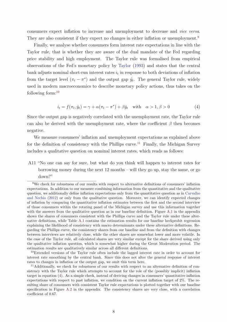
Regarding the Income Fisher equation, we observe, as already indicated by the sum-

mary statistics, rather little time variation. This is in line with our presumption that

the distinction between real and nominal income should be less dependent on changes

in macroeconomic conditions than the Phillips curve and the Taylor rule which may not

always be satisfied in reality.16 Over the last ten years the consistency of the public with

respect to the Income Fisher equation seems to follow an upward trend.

With respect to the Phillips curve and the Taylor rule, the consistency shares show

more time variation with a pronounced cyclical pattern especially for the share of con-

16Figure A.3 in the appendix depicts the shares of consumers consistent with the Phillips curve and theTaylor rule together with the periods when the Phillips curve trade-off and the Taylor rule concept whererealised in the changes in actual data 12 months ahead, rounded to the nearest integer. It seems thatboth were realised in the majority of periods in our sample. However, there are pronounced gaps at thebeginning of the sample period, when the U.S. economy was hit by stagflation and monetary policy wasless active. This could provide an explanation of the relatively low consistency shares observed duringthis period.

13

Table 3: Shares of Consumers with Consistent Expectations Regarding the Taylor Rule


All 0.46 0.46 0.08 0.23 0.63 238,396 13.47*** –

Male 0.46 0.45 0.08 0.23 0.69 106,349 0.42 0.14Female 0.46 0.46 0.08 0.24 0.65 131,542 -0.50 0.26

Age young 0.44 0.44 0.08 0.19 0.71 71,453 10.15*** 76.60***Age middle 0.46 0.46 0.08 0.24 0.70 88,146 -0.39 0.14Age old 0.47 0.47 0.09 0.20 0.68 77,329 -9.79*** 71.29***

Educ1 0.42 0.42 0.14 0.00 1.00 11,042 5.69*** 24.05***Educ2 0.42 0.42 0.11 0.14 0.80 17,527 9.11*** 61.80***Educ3 0.45 0.45 0.08 0.19 0.64 73,949 4.60*** 15.78***Educ4 0.46 0.46 0.08 0.22 0.67 56,170 0.76 0.39Educ5 0.47 0.47 0.09 0.21 0.74 46,924 -7.32*** 39.95***Educ6 0.48 0.48 0.11 0.17 0.72 30,038 -8.17*** 49.62***

Inc quint1 0.44 0.44 0.08 0.11 1.00 32,552 6.96*** 36.06***Inc quint2 0.45 0.46 0.09 0.22 0.68 38,675 3.69*** 10.13***Inc quint3 0.47 0.47 0.09 0.18 0.76 39,847 -0.75 0.45Inc quint4 0.46 0.46 0.09 0.18 0.77 48,349 0.68 0.36Inc quint5 0.48 0.48 0.10 0.20 0.76 50,470 -8.67*** 56.05***


sumers consistent with the Taylor rule. Recession periods denoted by the NBER, indicated

by the shaded areas, seem to impair the ability to form consistent expectations as they

correspond with downward dips in the consistency shares. Regarding the share of con-

sumers consistent with the Phillips curve, we observe that the share has fallen somewhat

since the beginning of the 2000s. This may be due to the relatively low and stable infla-

tion rate in recent years, which might make it more difficult for consumers to grasp the

Phillips curve trade-off.

Looking at the Taylor rule share specifically, we can report that people can forecast

rising and constant interest rates more accurately than falling interest rates during reces-

sions. This has been observed also by Carvalho and Nechio (2012) and for professional

forecasters. Within a tightening cycle the expectations become more in line with the

Taylor rule concept. The same holds true for unchanged interest rates. This asymmetric

response is not surprising as it may stem from people being unable to forecast recessions

are having problems absorbing negative news or policy reversals.

14

Table 4: Shares of Consumers with Consistent Expectations for All Three EconomicConcepts


All 0.06 0.06 0.02 0.02 0.15 223,143 19.16*** –

Male 0.07 0.07 0.03 0.02 0.17 99,539 -8.93*** 14.53***Female 0.06 0.06 0.02 0.01 0.15 123,237 8.89*** 14.39***

Age young 0.06 0.06 0.03 0.00 0.20 65,133 5.06*** 4.64**Age middle 0.06 0.06 0.02 0.01 0.16 83,472 1.69* 0.53Age old 0.07 0.07 0.03 0.01 0.21 73,283 -6.95*** 8.81***

Educ1 0.06 0.05 0.07 0.00 0.67 9,896 0.51 0.03Educ2 0.05 0.05 0.04 0.00 0.30 15,703 5.01*** 4.60**Educ3 0.06 0.06 0.02 0.00 0.17 68,603 8.84*** 14.24***Educ4 0.06 0.06 0.03 0.00 0.22 53,007 3.52*** 2.27Educ5 0.07 0.07 0.03 0.01 0.23 44,962 -7.60*** 10.51***Educ6 0.08 0.08 0.04 0.00 0.26 28,672 -10.74*** 21.04***

Inc quint1 0.06 0.06 0.03 0.00 0.20 32,181 3.29*** 1.99Inc quint2 0.06 0.05 0.03 0.00 0.19 37,637 6.13*** 6.87***Inc quint3 0.06 0.06 0.03 0.00 0.16 39,113 1.99** 0.71Inc quint4 0.06 0.06 0.03 0.00 0.18 47,219 2.03** 0.76Inc quint5 0.08 0.07 0.03 0.01 0.19 49,124 -11.65*** 24.75***


Finally, we further find some variation over time of the share of consumers consistent

with all three macroeconomic relations, albeit at a very low level. Again, we observe small

dips during recession periods.

While we are mainly interested in checking whether consumers believe in a Phillips

curve relationship or not, it makes sense to control for circumstances where the Phillips

curve trade-off should have been observed in practice, i.e. to control for periods when

demand or supply shock were dominating: In periods where demand shocks are expected

to dominate the economy, the aggregate demand (AD) curve with a positive relation

between inflation and unemployment shifts, so that rational consumers would adjust their

expectations along the Phillips curve. Hence, in these periods the Phillips curve trade-

off should be embodied in consumers’ expectations. Conversely, when supply shocks

are expected to dominate, rational consumers should move along the AD curve and,

hence, incorporate a positive correlation between inflation and unemployment in their

forecasts. As a tentative analysis of the question whether consumers behave in line with

15

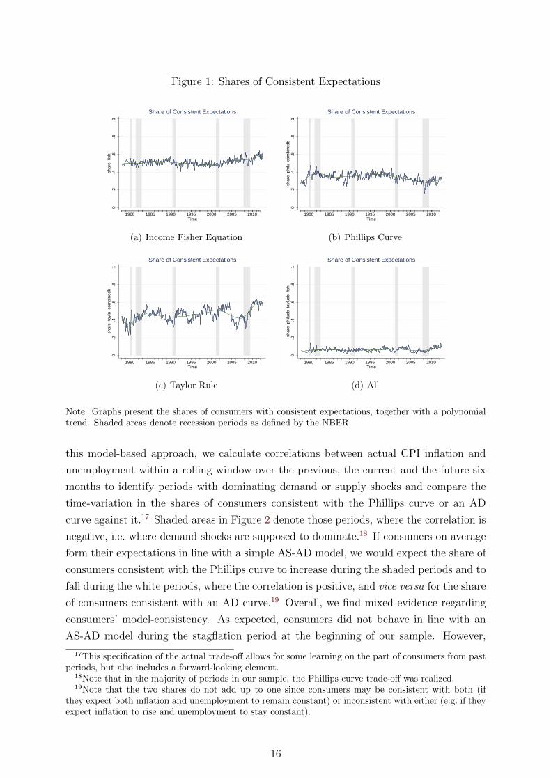
Figure 1: Shares of Consistent Expectations

0.2

.4.6

.81

shar

e_fis

h

1980 1985 1990 1995 2000 2005 2010Time

Share of Consistent Expectations

(a) Income Fisher Equation

0.2

.4.6

.81

shar

e_ph

ilu_c

ombi

nedb

1980 1985 1990 1995 2000 2005 2010Time


(b) Phillips Curve

0.2

.4.6

.81

shar

e_ta

ylu_

com

bine

db

1980 1985 1990 1995 2000 2005 2010Time


(c) Taylor Rule

0.2

.4.6

.81

shar

e_ph

ilucb

_tay

lucb

_fis

h

1980 1985 1990 1995 2000 2005 2010Time


(d) All

Note: Graphs present the shares of consumers with consistent expectations, together with a polynomialtrend. Shaded areas denote recession periods as defined by the NBER.

this model-based approach, we calculate correlations between actual CPI inflation and

unemployment within a rolling window over the previous, the current and the future six

months to identify periods with dominating demand or supply shocks and compare the

time-variation in the shares of consumers consistent with the Phillips curve or an AD

curve against it.17 Shaded areas in Figure 2 denote those periods, where the correlation is

negative, i.e. where demand shocks are supposed to dominate.18 If consumers on average

form their expectations in line with a simple AS-AD model, we would expect the share of

consumers consistent with the Phillips curve to increase during the shaded periods and to

fall during the white periods, where the correlation is positive, and vice versa for the share

of consumers consistent with an AD curve.19 Overall, we find mixed evidence regarding

consumers’ model-consistency. As expected, consumers did not behave in line with an

AS-AD model during the stagflation period at the beginning of our sample. However,

17This specification of the actual trade-off allows for some learning on the part of consumers from pastperiods, but also includes a forward-looking element.

18Note that in the majority of periods in our sample, the Phillips curve trade-off was realized.19Note that the two shares do not add up to one since consumers may be consistent with both (if

they expect both inflation and unemployment to remain constant) or inconsistent with either (e.g. if theyexpect inflation to rise and unemployment to stay constant).

16

Figure 2: Identification of the Phillips Curve

0.2

.4.6

.81

1980 1985 1990 1995 2000 2005 2010Time

Periods with negative Inflation−Unemployment trade−offShare consistent with the Phillips curveShare consistent with the AD curve

with the start of the disinflation in the early 1980s, we observe that the consistency share

regarding the Phillips curve is increases during shaded periods, and falls during periods,

where supply shocks might have dominated. This relation is less obvious during the

Great Moderation period, but emerges again from about 2006 onwards and throughout

the financial crisis.20

While we have shown that the shares of consistent consumers vary over time and

across demographic groups, it is also interesting to check if consumers stay consistent

between the first and the second interview of the rotating panel. Overall, between 45-

60% of consumers are either consistent or inconsistent in both interviews. This result

holds for all three concepts evaluated. Moreover, being consistent in the first interview

increases the likelihood of being consistent in the second interview by about 10-16% for a

representative consumer as defined below.21

Furthermore, we are interested in elaborating the reasons why expectations are not

consistent with the economic concepts. Looking at the Income Fisher relationship, we

observe that there are more inconsistent households that have negative real income ex-

pectations, but at the same time expect higher growth in nominal income than in prices,

than vice versa. Regarding the Phillips curve, those households that report prices to go

up, do not expect unemployment to go down. In fact, more than 85% of households who

20Notably, the share of consumers consistent with the AD curve is significantly higher than the corre-sponding Phillips curve share from about 2000 onwards.

21Estimation results from heckprobit models controlling for demographic factors are available from theauthors upon request.

17

expect inflation to go up, predict the unemployment rate to stay about the same or to be

higher in the next year. Dissecting the Taylor rule relationship implies that households

generally have problems with cases when nominal interest rates should be expected to

fall, either due to lower inflation or higher unemployment expectations. Especially, there

exist only weak links between expecting higher rates of unemployment and falling interest

rates.22 This is quite an interesting result. The Fed is known to put significant weight on

unemployment rates and economic growth relative to inflation as compared for instance

to the ECB. Therefore, one would expect that consumers in the U.S. would have less dif-

ficulties in understanding this relationship for a central bank that is as active in regarding

stabilizing unemployment as the Fed is.

4.2 Determinants of Consistency

In this section, we analyse possible macroeconomic determinants for the formation of

consistent expectations and check for effects of monetary policy communication. Specifi-

cally, we evaluate the relevance of macroeconomic conditions like inflation, unemployment,

money growth, short-run interest rates or the effect of being in a recession. We furthermore

investigate the inflation effect on consistency in more detail by distinguishing between in-

flation above and below the official target of 2%. Next, we check whether macroeconomic

effects differ between boom and recession periods. Finally, we analyse how changes in the

communication strategy of the Federal Reserve have affected consumers’ consistency with

macroeconomic concepts. All macroeconomic variables are included with one lag in order

to account for a publication lag.

We estimate probit models on the probability of forming theory-consistent expectations

regarding the Income Fisher equation, the Phillips curve, the Taylor rule as well as for all

three macroeconomic relations simultaneously. Tables 5-8 report marginal effects for our

set of determinants. In order to enable comparability across models, all marginal effects

are evaluated at a hypothetical “representative” consumer which we take to be male,

white, 40 years old, married, with a medium level of education and income and living

in the Northcentral region of the U.S. All models additionally include a wide range of

demographic controls including interaction terms thereof. Standard errors are calculated

with the δ method (Oehlert 1992).23

We thus specify a binary response model. The following variable is defined:

zi,t =

{1 if z∗i,t > 0

0 if z∗i,t ≤ 0, i = 1, 2, ..., N, (5)

22This result is in line with Carvalho and Nechio (2012).23Using standard errors clustered at the monthly level yield qualitatively the same results. Robust

standard errors are used here as there is no obvious dimension for clustering.

18

where z∗i,t is the latent variable that accounts for consumers’ theory-consistent expecta-

tions. Its discrete counterpart, zi,t, takes value one if the ith respondent formed theory-

consistent expectations in period t, and zero otherwise. The following latent process is

assumed:

z∗i,t = α1 + ytα2 + xi,tα3 + ui,t, (6)

where α1 is a constant, yt is the vector of macroeconomic variables, xi,t is a vector of

socio-demographic characteristics (namely gender, age, income, education, race, marital

status, location in the US and interaction terms between gender and education, race and

region, as well as income and marital status) and ui,t is normally distributed. We derive

the marginal partial effects from the estimation of Pr(zi,t= 1|hi,t) = Φ (hi,tξ), where Φ(·)is the CDF of the standard normal distribution, hi,t is the vector of covariates and ξ is a

vector of coefficients.

Since our dataset contains single survey interviews as well as interviews within the

rotating panel, estimations on the full dataset may lead to biased estimates due to a

sample selection problem. Moreover, additional sample selection might arise from non-

response bias, which might be higher for specific demographic groups.24 We therefore

account for possible attrition both with respect to non-response and with respect to being

selected into the rotating panel and estimate all models with a Heckman correction. Our

selection variable thus takes on the value of one for second interviews within the rotating

panel, conditional on response to the question on quantitative inflation expectations.25

Sample selection will only bias the estimates if the error terms of the outcome and of the

selection equation are significantly correlated as measured by the parameter ρ. Overall,

sample selection seems to have relatively small effects in our models since a Wald test

frequently cannot reject ρ = 0.

The marginal effects from the Heckman probit models in Table 5 imply that U.S. con-

sumers are less likely to form theory-consistent macroeconomic expectations with respect

to the Taylor rule in periods with high inflation levels and volatility, whereas the inflation

level is positively related to consistency with the Income Fisher equation. Interestingly,

a higher Federal Funds rate has a negative impact on consistency with both the Income

Fisher equation and the Taylor rule. Similarly, higher oil prices impair consumers’ ability

to form expectations consistent with the Phillips curve and jointly for all three relations.

Results regarding the effect of unemployment and money growth are less clear-cut. Fi-

nally, consumers show significantly lower degrees of consistency with the Phillips curve

and the Taylor rule in recession periods, while we find no significant business-cycle-effect

on consistency with the Income Fisher equation. This result is as expected, considering

24Specifically, we evaluate non-response to the question on quantitative inflation expectations. Weargue that this question might be perceived as being more demanding than the qualitative questions and,thus, more prone to non-response.

25Note that our Heckman probit estimates thus effectively account for only second interviews withinthe rotating panel.

19

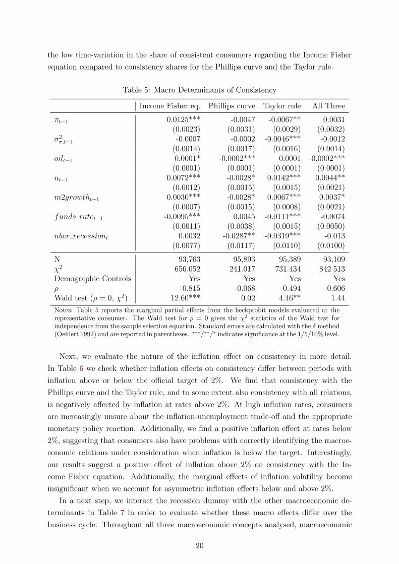
the low time-variation in the share of consistent consumers regarding the Income Fisher

equation compared to consistency shares for the Phillips curve and the Taylor rule.

Table 5: Macro Determinants of Consistency

Income Fisher eq. Phillips curve Taylor rule All Three

πt−1 0.0125*** -0.0047 -0.0067** 0.0031(0.0023) (0.0031) (0.0029) (0.0032)

σ2π,t−1 -0.0007 -0.0002 -0.0046*** -0.0012

(0.0014) (0.0017) (0.0016) (0.0014)oilt−1 0.0001* -0.0002*** 0.0001 -0.0002***

(0.0001) (0.0001) (0.0001) (0.0001)ut−1 0.0072*** -0.0028* 0.0142*** 0.0044**

(0.0012) (0.0015) (0.0015) (0.0021)m2growtht−1 0.0030*** -0.0028* 0.0067*** 0.0037*

(0.0007) (0.0015) (0.0008) (0.0021)funds ratet−1 -0.0095*** 0.0045 -0.0111*** -0.0074

(0.0011) (0.0038) (0.0015) (0.0050)nber recessiont 0.0032 -0.0287** -0.0319*** -0.013

(0.0077) (0.0117) (0.0110) (0.0100)

N 93,763 95,893 95,389 93,109χ2 656.052 241.017 731.434 842.513Demographic Controls Yes Yes Yes Yesρ -0.815 -0.068 -0.494 -0.606Wald test (ρ = 0, χ2) 12.60*** 0.02 4.46** 1.44

Notes: Table 5 reports the marginal partial effects from the heckprobit models evaluated at therepresentative consumer. The Wald test for ρ = 0 gives the χ2 statistics of the Wald test forindependence from the sample selection equation. Standard errors are calculated with the δ method(Oehlert 1992) and are reported in parentheses. ∗∗∗/∗∗/∗ indicates significance at the 1/5/10% level.

Next, we evaluate the nature of the inflation effect on consistency in more detail.

In Table 6 we check whether inflation effects on consistency differ between periods with

inflation above or below the official target of 2%. We find that consistency with the

Phillips curve and the Taylor rule, and to some extent also consistency with all relations,

is negatively affected by inflation at rates above 2%: At high inflation rates, consumers

are increasingly unsure about the inflation-unemployment trade-off and the appropriate

monetary policy reaction. Additionally, we find a positive inflation effect at rates below

2%, suggesting that consumers also have problems with correctly identifying the macroe-

conomic relations under consideration when inflation is below the target. Interestingly,

our results suggest a positive effect of inflation above 2% on consistency with the In-

come Fisher equation. Additionally, the marginal effects of inflation volatility become

insignificant when we account for asymmetric inflation effects below and above 2%.

In a next step, we interact the recession dummy with the other macroeconomic de-

terminants in Table 7 in order to evaluate whether these macro effects differ over the

business cycle. Throughout all three macroeconomic concepts analysed, macroeconomic

20

Table 6: Inflation Effects Above and Below 2% on Consistency


dummy π below2t−1 0.0247** -0.0347** -0.0418*** -0.0225**(0.0116) (0.0141) (0.0139) (0.0114)

πt−1 0.0127*** -0.0092*** -0.0134*** -0.0017(0.0029) (0.0034) (0.0033) (0.0026)

πt−1 ∗ dummy π below2t−1 -0.008 0.0278*** 0.0383*** 0.0220***(0.0056) (0.0068) (0.0070) (0.0067)

σ2π,t−1 -0.0009 0.002 -0.0042* 0.0012

(0.0020) (0.0025) (0.0024) (0.0019)σ2π,t−1 ∗ dummy π below2t−1 -0.0009 -0.0034 -0.0008 -0.0045*

(0.0025) (0.0033) (0.0031) (0.0027)oilt−1 0.0002*** -0.0002** 0.0001 -0.0002**

(0.0001) (0.0001) (0.0001) (0.0001)ut−1 0.0072*** -0.0011 0.0172*** 0.0058**

(0.0012) (0.0017) (0.0015) (0.0026)m2growtht−1 0.0026*** -0.0034*** 0.0056*** 0.0028

(0.0007) (0.0013) (0.0008) (0.0018)funds ratet−1 -0.0086*** 0.0054* -0.0091*** -0.0058

(0.0010) (0.0031) (0.0014) (0.0042)nber recessiont 0.0032 -0.0154 -0.0155 0.0006

(0.0085) (0.0140) (0.0111) (0.0132)

N 93,763 95,893 95,389 93,109χ2 649.422 265.052 770.548 1235.004Demographic Controls Yes Yes Yes Yesρ -0.814 -0.053 -0.435 -0.569Wald test (ρ = 0, χ2) 12.95*** 0.01 3.77** 1.26

Notes: Table 6 reports the marginal partial effects from the heckprobit models evaluated at the repre-sentative consumer. The Wald test for ρ = 0 gives the χ2 statistics of the Wald test for independencefrom the sample selection equation. Standard errors are calculated with the δ method (Oehlert 1992)and are reported in parentheses. ∗∗∗/∗∗/∗ indicates significance at the 1/5/10% level.

determinants have significantly different effects between boom and recession periods. In

line with our results in Table 6, we find that inflation increases the likelihood for con-

sumers to form expectations consistent with the Phillips curve during recessions (when

inflation rates typically fall). Interestingly, our results suggest that the effect of oil price

increases moves in the opposite direction to the inflation effect: Higher oil prices sig-

nificantly increase the likelihood of consistency with the Income Fisher equation during

recessions, while they have a detrimental effect on consistency with the Phillips curve or

the Taylor rule. This can be explained with rather strong oil price hikes during some of

the recessions in our sample period, especially during the oil price shocks of 1980 and

1990-91 and at the beginning of the financial crisis in 2008. Finally, both the marginal

effects of the Fed Funds rate and money supply growth seem relatively constant over the

business cycle.

21

Table 7: Recession Interaction Effects on Consistency


πt−1 0.0127*** -0.0068** -0.0111*** -0.0001(0.0029) (0.0028) (0.0029) (0.0014)

πt−1 ∗ nber recessiont -0.0065 0.0342*** 0.0135 0.0053(0.0116) (0.0115) (0.0115) (0.0060)

σ2π,t−1 0.0022 0.003 -0.0090*** 0.0003

(0.0023) (0.0022) (0.0023) (0.0012)σ2π,t−1 ∗ nber recessiont -0.0047 -0.0053 0.0097** -0.0007

(0.0040) (0.0039) (0.0039) (0.0020)oilt−1 -0.0001 -0.0002** 0.0002** -0.0002***

(0.0001) (0.0001) (0.0001) (0.0000)oilt−1 ∗ nber recessiont 0.0009*** -0.0010*** -0.0014*** -0.0002

(0.0003) (0.0003) (0.0003) (0.0002)ut−1 0.0069*** -0.0039*** 0.0164*** 0.0023***

(0.0015) (0.0014) (0.0014) (0.0008)ut−1 ∗ nber recessiont 0.0095 0.0208*** -0.0238*** -0.0015

(0.0080) (0.0079) (0.0080) (0.0040)m2growtht−1 0.0007 -0.0019** 0.0054*** 0.0016***

(0.0009) (0.0009) (0.0009) (0.0005)m2growtht−1 ∗ nber recessiont 0.0113 0.008 0.0005 0.0001

(0.0097) (0.0094) (0.0096) (0.0048)funds ratet−1 -0.0041*** 0.0034*** -0.0069*** -0.0025***

(0.0014) (0.0013) (0.0015) (0.0008)funds ratet−1 ∗ nber recessiont 0.0036 0.0073 0.0055 0.0029

(0.0051) (0.0050) (0.0051) (0.0026)nber recessiont -0.1517 -0.3397*** 0.0267 -0.0335

(0.1317) (0.1293) (0.1319) (0.0654)

N 93,763 95,893 95,389 93,109chi2 609.24 272.297 668.813 261.544Demographic Controls Yes Yes Yes Yesrho -0.019 -0.118 0.051 0.024Wald test (rho=0, chi2) 0.06 2.05 0.22 0.04

Notes: Table 7 reports the marginal partial effects from the heckprobit models evaluated at the represen-tative consumer. The Wald test for ρ = 0 gives the χ2 statistics of the Wald test for independence fromthe sample selection equation. Standard errors are calculated with the δ method (Oehlert 1992) and arereported in parentheses. ∗∗∗/∗∗/∗ indicates significance at the 1/5/10% level.

Finally, we test for an impact of changes in the communication strategy of the Fed

on consumers’ likelihood of forming consistent expectations. This is highly relevant, since

having a sound understanding of monetary policy increases the effectiveness of monetary

policy making. In an effort to improve the understanding of monetary policy and to guide

expectations of the public, central banks have, over the last two decades, established new

means of communication and transparency. To evaluate the success of these efforts, we

test to which extend the introduction of specific elements improved the understanding of

22

the public regarding monetary policy and helped them to form consistent expectations.

In order to analyse potential effects, we use the same set of macroeconomic determinants

used beforehand and amend this regression by the set of dummy variables representing

important milestones in the communication strategy of the Fed.26 Estimation results are

presented in Table 8.

As those milestones should influence the likelihood of being consistent with the Taylor

rule the most, we interpret these results first. We can report that the introduction of the

Beige book, the assessment of Risk, as well as the announcement of an explicit inflation

target helped to increase the propensity of consumers to form consistent expectations.

Regarding the relative size of the effects, the announcement of the explicit inflation target

stands out followed by the introduction of the Beige book. Both events may certainly be

characterized as major steps in the communication policy of the Federal Reserve. More-

over, given that the introduction of the explicit target has to be seen relative to the

introduction of the means beforehand, this result is remarkable in terms of size and signif-

icance. Furthermore, we can also observe that the publication of the voting record did not

help to improve the ability to form consistent expectations with respect to the Taylor rule.

This might not be surprising as this basically reflects a dimension of disagreement that

may not help to steer expectations in a specific direction. Interestingly, the introduction

of forward guidance in 2003 does not lead to significantly more people having consistent

Taylor rule expectations relative to the other means introduced beforehand.

Moreover, we also find effects of monetary policy communication on consistency with

the Income Fisher equation and the Phillips curve. The announcement of changes in

the Federal Funds target rate in February 1994 stands out as it had a positive effect

on consistency with the Phillips curve as well as consistency with all three concepts

simultaneously. Moreover, the announcement of the explicit inflation target in January

2012, in addition to improving consistency with the Taylor rule, also significantly raised

the likelihood of consistency with the Income Fisher equation. Notably, the effect has

a similar size for both relations. Additionally, we find positive effects of the publication

of votes, the introduction of forward guidance and the press conference on consumers’

likelihood of correctly distinguishing between real and nominal expected income.27

26Middeldorp (2011) also incorporates dummy variables to control for important milestones of commu-nication.

27We also check for the potentially heterogeneous impact of communication effects across demographicgroups by varying different characteristics of our representative agent when calculating marginal effects.While we find the differences across demographic groups to be small, and generally not significant, westill observe some patterns: For example, regarding the Taylor rule the effect of the introduction of theinflation target is higher for men, poorer consumers, and those with less education. On the contrary,regarding the effect of announcing the Federal Funds target on consistency with the Phillips curve, wefind that it is higher for wealthier and more educated households. The results are available from theauthors upon request. We furthermore investigate if our results hold also if we add a time trend and ifwe estimate the same equation with only a subset of dummy variables, i.e. using only the events BeigeBook, Federal Funds Target and the explicit announcement of the inflation target. The results remainvirtually the same.

23

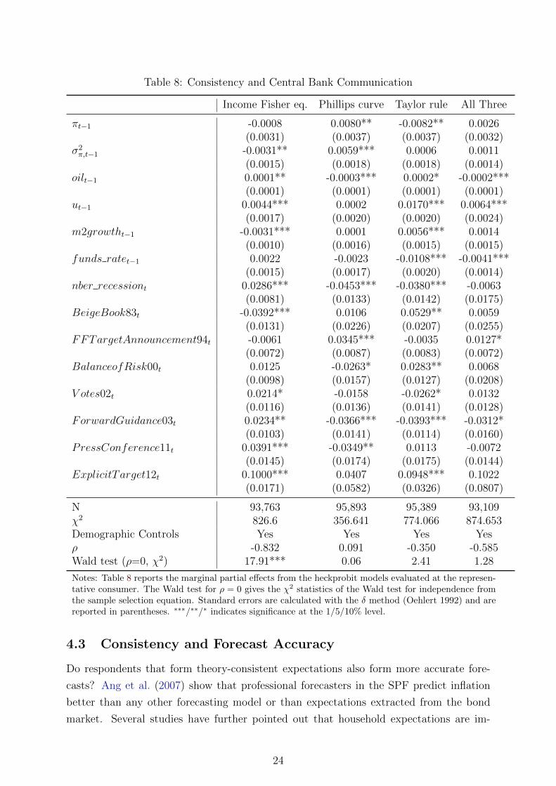
Table 8: Consistency and Central Bank Communication


πt−1 -0.0008 0.0080** -0.0082** 0.0026(0.0031) (0.0037) (0.0037) (0.0032)

σ2π,t−1 -0.0031** 0.0059*** 0.0006 0.0011

(0.0015) (0.0018) (0.0018) (0.0014)oilt−1 0.0001** -0.0003*** 0.0002* -0.0002***

(0.0001) (0.0001) (0.0001) (0.0001)ut−1 0.0044*** 0.0002 0.0170*** 0.0064***

(0.0017) (0.0020) (0.0020) (0.0024)m2growtht−1 -0.0031*** 0.0001 0.0056*** 0.0014

(0.0010) (0.0016) (0.0015) (0.0015)funds ratet−1 0.0022 -0.0023 -0.0108*** -0.0041***

(0.0015) (0.0017) (0.0020) (0.0014)nber recessiont 0.0286*** -0.0453*** -0.0380*** -0.0063

(0.0081) (0.0133) (0.0142) (0.0175)BeigeBook83t -0.0392*** 0.0106 0.0529** 0.0059

(0.0131) (0.0226) (0.0207) (0.0255)FFTargetAnnouncement94t -0.0061 0.0345*** -0.0035 0.0127*

(0.0072) (0.0087) (0.0083) (0.0072)BalanceofRisk00t 0.0125 -0.0263* 0.0283** 0.0068

(0.0098) (0.0157) (0.0127) (0.0208)V otes02t 0.0214* -0.0158 -0.0262* 0.0132

(0.0116) (0.0136) (0.0141) (0.0128)ForwardGuidance03t 0.0234** -0.0366*** -0.0393*** -0.0312*

(0.0103) (0.0141) (0.0114) (0.0160)PressConference11t 0.0391*** -0.0349** 0.0113 -0.0072

(0.0145) (0.0174) (0.0175) (0.0144)ExplicitTarget12t 0.1000*** 0.0407 0.0948*** 0.1022

(0.0171) (0.0582) (0.0326) (0.0807)

N 93,763 95,893 95,389 93,109χ2 826.6 356.641 774.066 874.653Demographic Controls Yes Yes Yes Yesρ -0.832 0.091 -0.350 -0.585Wald test (ρ=0, χ2) 17.91*** 0.06 2.41 1.28

Notes: Table 8 reports the marginal partial effects from the heckprobit models evaluated at the represen-tative consumer. The Wald test for ρ = 0 gives the χ2 statistics of the Wald test for independence fromthe sample selection equation. Standard errors are calculated with the δ method (Oehlert 1992) and arereported in parentheses. ∗∗∗/∗∗/∗ indicates significance at the 1/5/10% level.

4.3 Consistency and Forecast Accuracy

Do respondents that form theory-consistent expectations also form more accurate fore-

casts? Ang et al. (2007) show that professional forecasters in the SPF predict inflation

better than any other forecasting model or than expectations extracted from the bond

market. Several studies have further pointed out that household expectations are im-

24

portant from the perspective of monetary policy. We study the accuracy of quantitative

inflation expectations of consistent and non-consistent consumers and compare them to

the median forecast of the SPF. Thus, we evaluate if we can systematically extract in-

dividuals – not only based on demographic characteristics – that produce more accurate

inflation forecasts.

We start the analysis by plotting the average absolute forecast errors (AFEs) of theory-

consistent consumers relative to the AFEs of consumers with non-consistent expectations

in Figure 3, where summary statistics of the relative shares are given in Table 9. A rela-

tive share below one means that theory-consistent consumers in a given period have lower

absolute forecast errors than non-consistent consumers, and vice versa. In most periods,

consistent consumers produce lower AFEs with respect to inflation. An exception is the

period at the beginning of our sample where consumers that have theory-consistent expec-

tations perform worse than non-consistent consumers, especially in the case of consistency

with the Phillips curve and the Taylor rule. We have to bear in mind that those respon-

dents surveyed in the late 1970’s and early 1980’s experienced stagflation and non-active

monetary policy and that in most of these early periods neither the Phillips curve relation-

ship nor the Taylor rule held in reality as shown in Figure A.3 in the appendix. As shown

in Figure 1 in section 4.1, we also find a relatively lower share of consumers forming con-

sistent expectations during this period, which one would expect when consumers expect

stagflation. With the appointment of Volcker as the Fed chairman at the end of 1979, more

consumers started to forecast in a theory-consistent way and their forecasts became more

accurate compared to consumers giving non-consistent forecasts. Especially with respect

to the Phillips curve and the Taylor rule, we observe consumers with theory-consistent

expectations in recent years markedly improved their inflation forecasts in relation to the

non-consistent consumers.

Overall, respondents who correctly distinguish between nominal and real variables and

those that have expectations consistent with the Taylor rule produce forecasts that have on

average 1% lower AFEs than non-consistent consumers. While this difference is relatively

small, respondents who form consistent expectations with respect to the Phillips curve

differ much more in their forecast accuracy compared to the respective non-consistent

samples and have 20% lower AFEs. Consumers whose expectations are consistent with

all three principles have on average 12% lower AFEs than the non-consistent consumers.

Note that the improvement in forecast accuracy of consistent consumers is even larger

when we compare the median values. In Figure 3 we can also observe that the variance is

relatively high with the highest variance for consistency with all three principles. Summary

statistics are provided in Table 9.

Next, we evaluate the distance of the AFEs of consistent and non-consistent forecasts

to the AFEs of the SPF, shown in Figure 4 with summary statistics in Table 10. As the

difference approaches zero, consumers’ forecast accuracy regarding inflation approaches

that of the SPF. A positive difference means that consumers have higher AFEs than

25

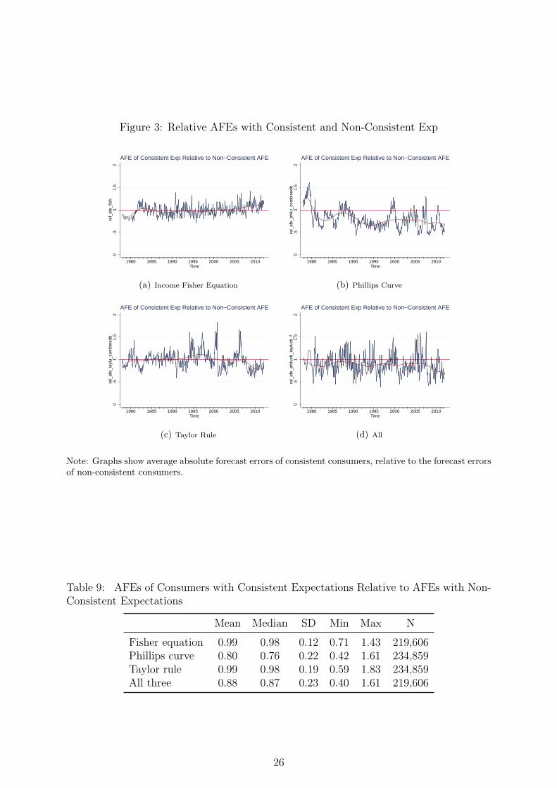
Figure 3: Relative AFEs with Consistent and Non-Consistent Exp

0.5

11.

52

rel_

afe_

fish

1980 1985 1990 1995 2000 2005 2010Time

AFE of Consistent Exp Relative to Non−Consistent AFE

(a) Income Fisher Equation0

.51

1.5

2re

l_af

e_ph

ilu_c

ombi

nedb

1980 1985 1990 1995 2000 2005 2010Time


(b) Phillips Curve

0.5

11.

52

rel_

afe_

tayl

u_co

mbi

nedb

1980 1985 1990 1995 2000 2005 2010Time


(c) Taylor Rule

0.5

11.

52

rel_

afe_

philu

cb_t

aylu

cb_f

1980 1985 1990 1995 2000 2005 2010Time


(d) All

Note: Graphs show average absolute forecast errors of consistent consumers, relative to the forecast errorsof non-consistent consumers.

Table 9: AFEs of Consumers with Consistent Expectations Relative to AFEs with Non-Consistent Expectations

Mean Median SD Min Max N

Fisher equation 0.99 0.98 0.12 0.71 1.43 219,606Phillips curve 0.80 0.76 0.22 0.42 1.61 234,859Taylor rule 0.99 0.98 0.19 0.59 1.83 234,859All three 0.88 0.87 0.23 0.40 1.61 219,606

26

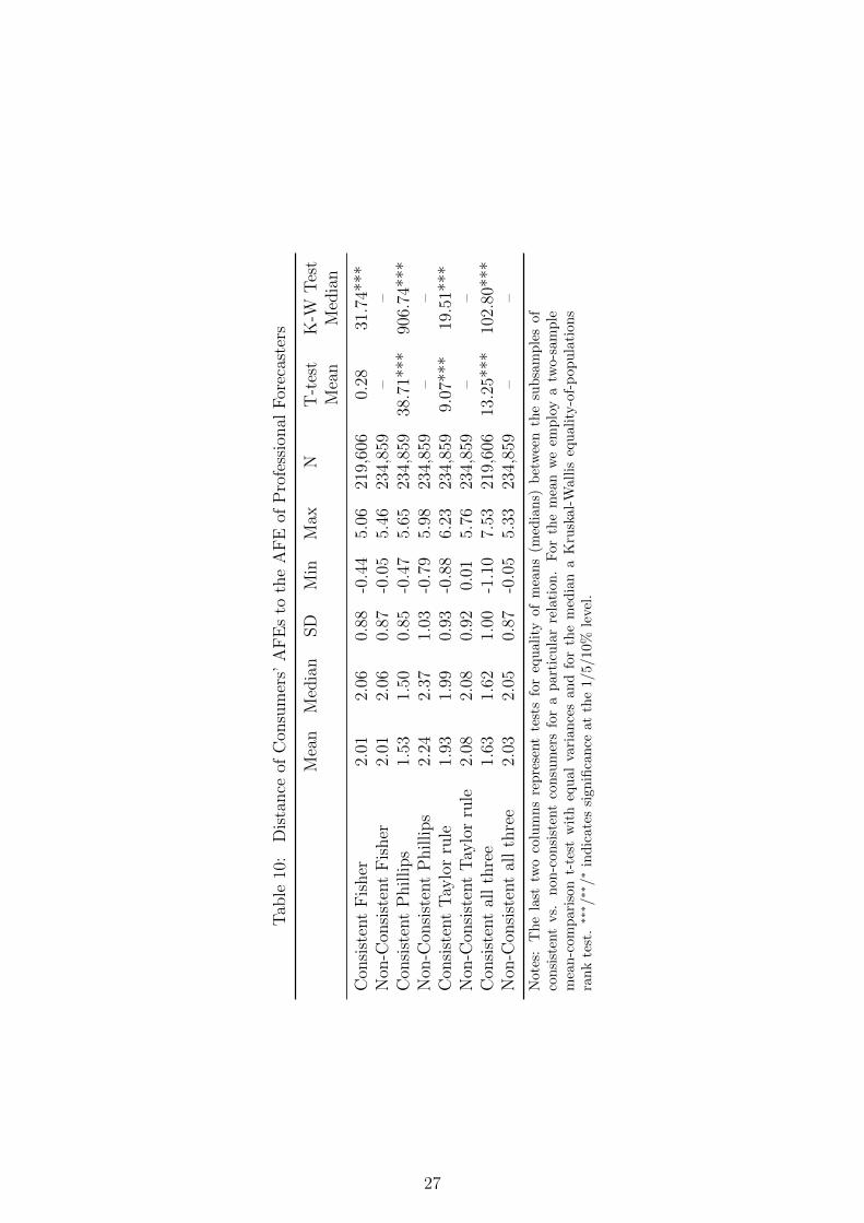
Tab

le10

:D

ista

nce

ofC

onsu

mer

s’A

FE

sto

the

AF

Eof

Pro

fess

ional

For

ecas

ters

Mea

nM

edia

nSD

Min

Max

NT

-tes

tK

-WT

est

Mea

nM

edia

n

Con

sist

ent

Fis

her

2.01

2.06

0.88

-0.4

45.

0621

9,60

60.

2831

.74*

**N

on-C

onsi

sten

tF

isher

2.01

2.06

0.87

-0.0

55.

4623

4,85

9–

–C

onsi

sten

tP

hillips

1.53

1.50

0.85

-0.4

75.

6523

4,85

938

.71*

**90

6.74

***

Non

-Con

sist

ent

Phillips

2.24

2.37

1.03

-0.7

95.

9823

4,85

9–

–C

onsi

sten

tT

aylo

rru

le1.

931.

990.

93-0

.88

6.23

234,

859

9.07

***

19.5

1***

Non

-Con

sist

ent

Tay

lor

rule

2.08

2.08

0.92

0.01

5.76

234,

859

––

Con

sist

ent

all

thre

e1.

631.

621.

00-1

.10

7.53

219,

606

13.2

5***

102.

80**

*N

on-C

onsi

sten

tal

lth

ree

2.03

2.05

0.87

-0.0

55.

3323

4,85

9–

–

Not

es:

Th

ela

sttw

oco

lum

ns

repre

sent

test

sfo

req

uality

of

mea

ns

(med

ian

s)b

etw

een

the

subsa

mp

les

of

consi

sten

tvs.

non

-con

sist

ent

con

sum

ers

for

apart

icu

lar

rela

tion

.F

or

the

mea

nw

eem

plo

ya

two-s

am

ple

mea

n-c

ompar

ison

t-te

stw

ith

equ

alva

rian

ces

an

dfo

rth

em

edia

na

Kru

skal-

Wallis

equality

-of-

popu

lati

ons

ran

kte

st.∗∗∗ /∗∗/∗

indic

ates

sign

ifica

nce

at

the

1/5/10%

leve

l.

27

Figure 4: Consistent and Non-Consistent AFEs of Consumers vs. AFEs in the SPF

02

46

1980 1985 1990 1995 2000 2005 2010Time

Difference of AFEs to the AFE of Professional Forecasters

(a) Income Fisher Equation

−2

02

46

1980 1985 1990 1995 2000 2005 2010Time


(b) Phillips Curve

−2

02

46

1980 1985 1990 1995 2000 2005 2010Time


(c) Taylor Rule

−2

02

46

8

1980 1985 1990 1995 2000 2005 2010Time


(d) All

Note: Black lines denote differences in AFEs of consistent consumers, red dotted lines denote differencesin AFEs of non-consistent consumers.

professional forecasters, while a negative difference means that consumers beat the SPF

forecast on average. As one would expect, in most periods consumers’ AFEs are higher

than the SPF errors for both consistent and non-consistent consumers, where the overall

median AFE from the Michigan survey is 135% higher than the median AFE of the SPF.

As shown in Table 10, consumers with expectations consistent with the Income Fisher

equation produce AFEs that are 2.01 inflation points higher than those in the SPF, while

AFEs from forecasts consistent with the Phillips curve and the Taylor rule are 1.53 and

1.93 points higher, respectively. For comparison the average absolute forecasts error in

the SPF is 1.27 inflation points.

Nevertheless, there exist periods where consumers that form consistent forecasts out-

perform the SPF. These are most evident in the first half of the 1980s and in 2008; the

latter especially for consistency with the Phillips curve as well as with all three principles.

Moreover, consumers with consistent expectations are consistently better able to match

the SPF forecast accuracy than their non-consistent counterparts. This is especially true

in the later part of the sample period, after the Volcker disinflation and the beginning

of an active monetary policy regime in the U.S. As shown in Table 10, these differences

28

are statistically significant in almost all cases, meaning that consistency with economic

concepts on average moves consumers’ inflation forecasts closer to professionals’ estimates.

5 Conclusion

Expectations are of key relevance for macroeconomic outcomes. While many papers have

investigated the properties of expectations of individual series in depth, there is almost

no evidence on whether expectations on several macroeconomic aggregates are formed

consistent with important economic concepts.

This paper addresses this research gap by calculating the share of people that form

consistent expectations regarding the Taylor rule, the Phillips curve and the Income Fisher

equation. In addition, we explore how this share of consistent consumers changes over

time and how it is affected both by macroeconomic variables and by the communication

policy of the Federal Reserve, and finally check if people benefit from having consistent

expectations in terms of reduced inflation forecast errors.

We find that 50% of the surveyed U.S. population form expectations in line with the

Income Fisher equation, while 46% incorporate the Taylor rule relationship into their

expectations. Furthermore, 34% correctly infer the Phillips curve trade-off. While this

share is relatively time-invariant for the Income Fisher equation, it seems to be more

business-cycle-dependent for the Phillips curve and the Taylor rule. When looking at the

heterogeneity across socioeconomic characteristics, we find some variation for all concepts

considered, especially for the consistency with the Income Fisher equation.

In addition, we show that having consistent expectations is affected by a certain set

of macro determinants. In particular, higher inflation above 2% decreases the probability

of forming consistent expectations with respect to the Phillips curve and the Taylor rule,

while the effect is positive for consistency with the Income Fisher equation. Also, during

recessions people have problems forming consistent expectations regarding the Phillips

curve trade-off and the Taylor rule relationship. Moreover, consistency with respect to all

macroeconomic concepts analysed was affected significantly by changes in the communi-

cation strategy of the Federal Reserve. We find that consistency with the Taylor rule and

with the Income Fisher equation are most strongly positively affected by improvements in

communication and transparency, where the strongest effect is found for the introduction

of the official inflation target in January 2012. Finally, we can show that having consis-

tent expectations benefits consumers. Investigating their inflation forecast accuracy, we

report that consumers make better inflation forecasts and are closer to the SPF forecast

accuracy if they have consistent expectations.

This paper offers interesting insights regarding the formation process of expectations

by consumers. We contribute to the literature by testing for the consistency of economic

concepts instead of only analysing the rationality of individual time series. Furthermore,

the result that people benefit from having consistent expectations and at the same time

29

have problems with recession periods may call for policy actions. Nevertheless, we can

show that the already introduced measures of monetary policy communication have had

significantly positive effects on the likelihood of forming consistent expectations. Hence,

our results could give further reasons for a clear communication by monetary and fiscal

authorities especially during recession periods and, thus, could give further motivation for

the recently popular measures of forward guidance. Additional benefit might be gained

by targeting specific demographic groups such as older, less educated and lower income

groups as this could increase overall economic literacy in the population. Finally, our

result that consistent consumers have lower inflation forecast errors could be used to

improve forecasting methods which incorporate consumer expectations.

References

Anderson, R. D., R. Becker, and D. R. Osborn (2010). Heterogeneity in Consumers’

Learning about Inflation. Newcastle Discussion Papers in Economics 2.

Andrade, P. and H. Le Bihan (2010). Inattentive professional forecasters. Working papers

307, Banque de France.

Ang, A., G. Bekaert, and M. Wei (2007). Do macro variables, asset markets, or surveys

forecast inflation better? Journal of Monetary Economics 54 (4), 1163–1212.

Armantier, O., W. Bruine de Bruin, G. Topa, W. van der Klaauw, and B. Zafar (2011).

Inflation expectations and behavior: Do survey respondents act on their beliefs? Federal

Reserve Bank of New York Staff Reports 509.

Bachmann, R., T. O. Berg, and E. R. Sims (2014). Inlation expectations and readiness

to spend: Cross-sectional evidence. mimeo.

Baghestani, H. and S. Kherfi (2008). How well do U.S. consumers predict the direction

of change in interest rates? The Quarterly Journal of Economics and Finance 48 (4),

725–732.

Blanchflower, D. G. and R. Kelly (2008). Macroeconomic literacy, numeracy and the

implications for monetary policy. Working Paper Bank of England .

Blinder, A. S., M. Ehrmann, M. Fratzscher, J. D. Haan, and D.-J. Jansen (2008, De-

cember). Central bank communication and monetary policy: A survey of theory and

evidence. Journal of Economic Literature 46 (4), 910–45.

Branch, W. A. (2004). The theory of rationally heterogeneous expectations: Evidence

from survey data on inflation expectations. Economic Journal 114 (497), 592–621.

30

Branch, W. A. (2007). Sticky information and model uncertainty in survey data on

inflation expectations. Journal of Economic Dynamics and Control 31 (1), 245–276.

Bryan, M. F. and G. Venkatu (2001, Oct.). The demographics of inflation opinion surveys.

Economic Commentary (15).

Burke, M. A. and M. Manz (2011). Economic Literacy and Inflation Expectations: Ev-

idence from a Laboratory Experiment. Federal Reserve Bank of Boston Public Policy

Discussion Paper 11-8.

Carlson, J. B., B. Craig, P. Higgins, and W. R. Melick (2006). Fomc communications and

the predictability of near-term policy decisions. Economic Commentary (Jun).

Carlstrom, C. T. and T. S. Fuerst (2008). Explaining apparent changes in the phillips

curve: the great moderation and monetary policy. Economic Commentary (Feb).

Carroll, C. D. and W. E. Dunn (1997). Unemployment expectations, jumping (s,s) trig-

gers, and household balance sheets. NBER Macroeconomics Annual 12, 165–230.

Carvalho, C. and F. Nechio (2012). Do People Understand Monetary Policy? Federal

Reserve Bank of San Francisco Working Paper 2012-01.

Coibion, O. and Y. Gorodnichenko (2010). Information Rigidity and the Expectations

Formation Process: A Simple Framework and New Facts. NBER Working Paper 16537.

Coibion, O. and Y. Gorodnichenko (2012). What Can Survey Forecasts Tell Us About

Information Rigidities? Journal of Political Economy 120 (1), 116–159.

Curtin, R. (2003). Unemployment expectations: The impact of private information on

income uncertainty. Review of Income and Wealth 49 (4), 539–554.

Dotsey, M., S. Fujita, and T. Stark (2011). Do phillips curves conditionally help to forecast

inflation? Federal Reserve Bank of Philadelphia Working Paper 11-40.

Ehrmann, M. and M. Fratzscher (2007, 03). Communication by central bank commit-

tee members: Different strategies, same effectiveness? Journal of Money, Credit and

Banking 39 (2-3), 509–541.

Faust, J. and J. H. Wright (2013). Forecasting inflation. In G. Elliott and A. Timmermann

(Eds.), Handbook of Economic Forecasting, Volume 2A. Elsevier.

Fendel, R., M. Frenkel, and J.-C. Rulke (2011b). ‘ex-ante’ Taylor rules – newly discovered

evidence from the G7 countries. Journal of Macroeconomics 33 (2), 224 – 232.

Fendel, R., E. Lis, and J.-C. Rulke (2011a). Does the financial market believe in the

phillips curve? evidence from the G7 countries. Journal of Forecasting 30, 268 – 287.

31

Hayo, B. and M. Neuenkirch (2010). Do Federal Reserve communications help predict

Federal Funds target rate decisions? Journal of Macroeconomics 32 (4), 1014 – 1024.

Jonung, L. (1981, December). Perceived and expected rates of inflation in sweden. Amer-

ican Economic Review 71 (5), 961–68.

Mankiw, N. G., R. Reis, and J. Wolfers (2004). Disagreement about inflation expectations.

In NBER Macroeconomics Annual 2003, Volume 18, pp. 209–248.

Middeldorp, M. (2011). FOMC communication policy and the accuracy of Fed Funds

futures. Staff Reports 491, Federal Reserve Bank of New York.

Oehlert, G. W. (1992). A note on the delta method. The American Statistician 46 (1),

pp. 27–29.

Pfajfar, D. and E. Santoro (2009). Asymmetries in Inflation Expectations across Sociode-

mographic Groups. mimeo.

Phillips, A. (1958). The Relation between Unemployment and the Rate of Change of

Money Wage Rates in the United Kingdom, 1861-1857. Economica 25 (100), 283–299.

Samuelson, P. A. and R. M. Solow (1960). Problem of Achieving and a Maintaining Stable

Price Level: Analytical Aspects of Anti-Inflation Policy . The American Economic

Review 50 (2), 177–194.

Souleles, N. S. (2004). Expectations, heterogenous forecast errors, and consumption:

Micro evidence from the michigan consumer sentiment surveys. Journal of Money,

Credit, and Banking 36 (1), 40–72.

Stock, J. H. and M. W. Watson (2008, September). Phillips curve inflation forecasts.

NBER Working Paper 14322.

Sturm, J.-E. and J. Haan (2011, April). Does central bank communication really lead to

better forecasts of policy decisions? new evidence based on a Taylor rule model for the

ECB. Review of World Economics (Weltwirtschaftliches Archiv) 147 (1), 41–58.

Taylor, J. B. (1993). Discretion versus policy rules in practice. Carnegie-Rochester Con-

ference Series on Public Policy 39, 195–214.

Tortorice, D. L. (2012). Unemployment Expectations and the Business Cycle. The B.E.

Journal of Macroeconomics (Topics) 12 (1), 1.

6 Appendix

32

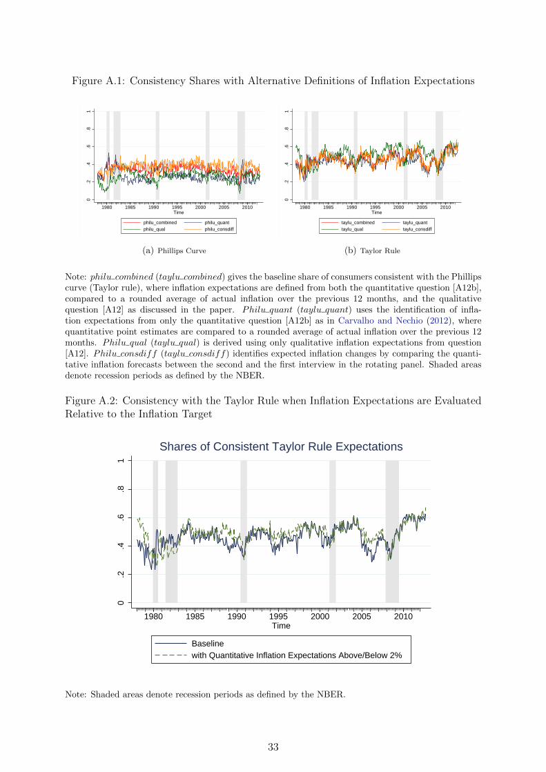
Figure A.1: Consistency Shares with Alternative Definitions of Inflation Expectations0

.2.4

.6.8

1

1980 1985 1990 1995 2000 2005 2010Time

philu_combined philu_quantphilu_qual philu_consdiff

(a) Phillips Curve

0.2

.4.6

.81

1980 1985 1990 1995 2000 2005 2010Time

taylu_combined taylu_quanttaylu_qual taylu_consdiff

(b) Taylor Rule

Note: philu combined (taylu combined) gives the baseline share of consumers consistent with the Phillipscurve (Taylor rule), where inflation expectations are defined from both the quantitative question [A12b],compared to a rounded average of actual inflation over the previous 12 months, and the qualitativequestion [A12] as discussed in the paper. Philu quant (taylu quant) uses the identification of infla-tion expectations from only the quantitative question [A12b] as in Carvalho and Nechio (2012), wherequantitative point estimates are compared to a rounded average of actual inflation over the previous 12months. Philu qual (taylu qual) is derived using only qualitative inflation expectations from question[A12]. Philu consdiff (taylu consdiff) identifies expected inflation changes by comparing the quanti-tative inflation forecasts between the second and the first interview in the rotating panel. Shaded areasdenote recession periods as defined by the NBER.

Figure A.2: Consistency with the Taylor Rule when Inflation Expectations are EvaluatedRelative to the Inflation Target

0.2

.4.6

.81

1980 1985 1990 1995 2000 2005 2010Time

Baselinewith Quantitative Inflation Expectations Above/Below 2%

Shares of Consistent Taylor Rule Expectations

Note: Shaded areas denote recession periods as defined by the NBER.

33

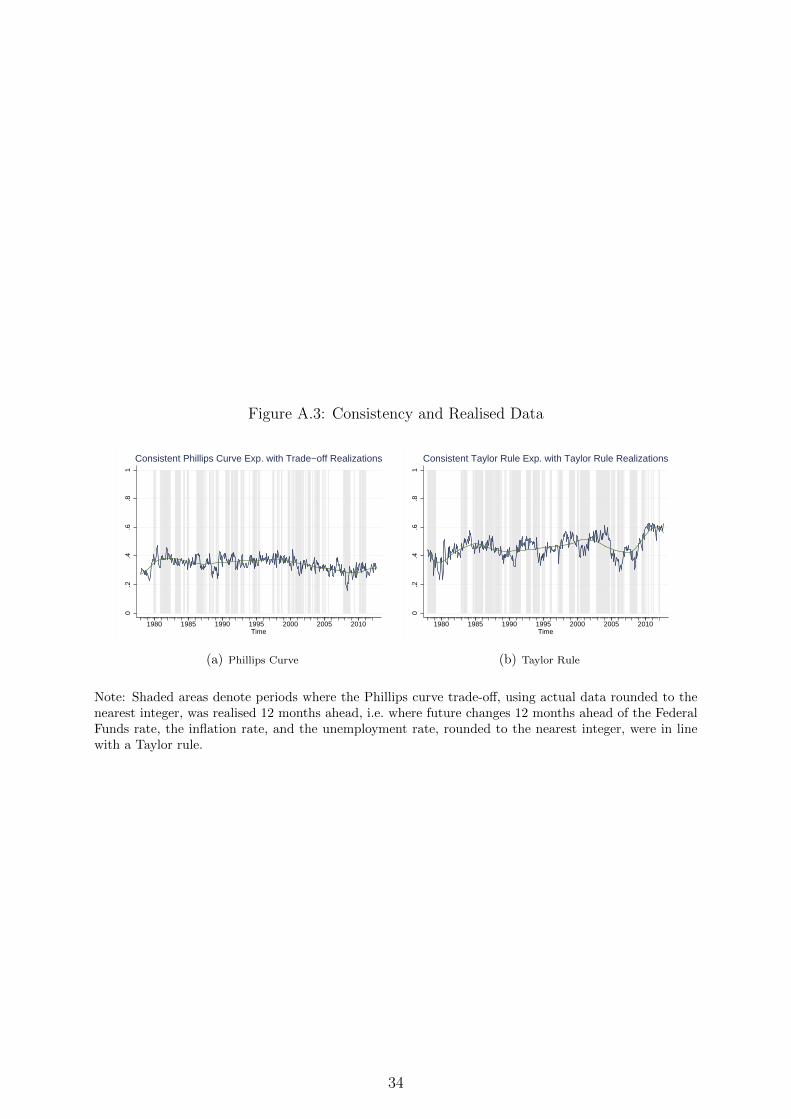
Figure A.3: Consistency and Realised Data

0.2

.4.6

.81

1980 1985 1990 1995 2000 2005 2010Time

Consistent Phillips Curve Exp. with Trade−off Realizations

(a) Phillips Curve

0.2

.4.6

.81

1980 1985 1990 1995 2000 2005 2010Time

Consistent Taylor Rule Exp. with Taylor Rule Realizations

(b) Taylor Rule

Note: Shaded areas denote periods where the Phillips curve trade-off, using actual data rounded to thenearest integer, was realised 12 months ahead, i.e. where future changes 12 months ahead of the FederalFunds rate, the inflation rate, and the unemployment rate, rounded to the nearest integer, were in linewith a Taylor rule.

34

Tab

leA

.1:

Rob

ust

nes

sC

hec

ks

Hec

kpro

bit

Model

sw

ith

Diff

eren

tId

enti

fica

tion

sof

Inflat

ion

Exp

ecta

tion

s

Phillips

curv

eT

aylo

rru

lephilucombined

philuquant

philuqual

philuconsdiff

taylucombined

tayluquant

tayluqual.

tayluconsdiff

(bas

elin

e)(b

asel

ine)

πt−

1-0

.004

70.

0078

***

-0.0

039

-0.0

129*

**-0

.006

7**

-0.0

091*

**-0

.014

0***

0.00

27(0

.003

1)(0

.002

9)(0

.004

3)(0

.002

6)(0

.002

9)(0

.003

3)(0

.004

2)(0

.002

6)σ2 π,t−1

-0.0

002

0.00

97**

*0.

0064

***

0.00

2-0

.004

6***

-0.0

060*

**0.

0027

-0.0

042*

**(0

.001

7)(0

.001

7)(0

.001

9)(0

.001

6)(0

.001

6)(0

.001

7)(0

.001

9)(0

.001

6)oil t−1

-0.0

002*

**-0

.000

6***

-0.0

003*

*-0

.000

2**

0.00

010.

0003

***

-0.0

001

-0.0

003*

**(0

.000

1)(0

.000

1)(0

.000

1)(0

.000

1)(0

.000

1)(0

.000

1)(0

.000

1)(0

.000

1)ut−

1-0

.002

8*-0

.004

1***

0.01

65*

-0.0

034*

*0.

0142

***

0.01

00**

*-0

.024

2***

0.01

14**

*(0

.001

5)(0

.001

2)(0

.009

8)(0

.001

4)(0

.001

5)(0

.001

4)(0

.008

5)(0

.001

4)m

2growtht−

1-0

.002

8*-0

.005

0***

-0.0

048*

*-0

.002

4**

0.00

67**

*0.

0045

***

-0.0

013

0.00

66**

*(0

.001

5)(0

.000

7)(0

.002

2)(0

.001

1)(0

.000

8)(0

.001

0)(0

.002

2)(0

.000

8)fundsratet−

10.

0045

-0.0

011

-0.0

060.

0036

-0.0

111*

**-0

.005

3**

-0.0

155*

**-0

.012

6***

(0.0

038)

(0.0

022)

(0.0

058)

(0.0

025)

(0.0

015)

(0.0

025)

(0.0

052)

(0.0

014)

nberrecessiont

-0.0

287*

*0.

0388

***

-0.0

338*

**-0

.041

4***

-0.0

319*

**-0

.030

8**

-0.0

472*

**-0

.008

8(0

.011

7)(0

.011

1)(0

.013

0)(0

.008

7)(0

.011

0)(0

.012

9)(0

.013

1)(0

.010

2)

N95

893

9589

395

893

9589

395

389

9538

995

389

9538

9χ2

241.

017

409.

629

1127

.469

259.

314

731.

434

365.

214

1108

.565

629.

738

Dem

ogra

phic

Con

trol

sY

esY

esY

esY

esY

esY

esY

esY

esρ

-0.0

680.

119

-0.2

900.

104

-0.4

94-0

.471

-0.3

21-0

.590

Wal

dte

st(ρ

=0,χ2)

0.02

0.18

1.32

0.12

4.46

**2.

272.

575.

01**

Not

es:

For

expla

nat

ion

ofth

ed

efinit

ions,

see

not

esto

Fig

ure

A.1

.T

ab

leA

.1re

port

sth

em

arg

inal

part

ial

effec

tsfr

om

the

hec

kpro

bit

mod

els

evalu

ate

dat

the

repre

senta

tive

consu

mer

.T

he

Wal

dte

stfo

rρ

=0

gives

theχ2

stati

stic

sof

the

Wald

test

for

indep

end

ence

from

the

sam

ple

sele

ctio

neq

uati

on

.Sta

ndard

erro

rsar

eca

lcu

late

dw

ith

theδ

met

hod

(Oeh

lert

1992

)an

dar

ere

port

edin

pare

nth

eses

.∗∗∗ /∗∗/∗

indic

ate

ssi

gnifi

can

ceat

the

1/5/10%

leve

l.

35

are consumer expectations theory- consistent? the … us to identify patterns in consumers’...

Documents