are labor markets segmented in argentina? a seminparametric
TRANSCRIPT

Are Labor Markets Segmented in Argentina?
A Semiparametric Approach
Sangeeta Pratap
Instituto Tecnologico Autonomo de Mexico
Erwan Quintin
Federal Reserve Bank of Dallas
January 13, 2003
∗Email: [email protected] and [email protected] wish to thank Steve Bronars, Daniel Hammermesh, Hugo Hopenhayn, David Kaplan, Torsten Perssonas well as seminar participants at the University of Texas, Austin, the University of Montreal and SouthernMethodist University for valuable comments. We are also grateful to Fernanda Fenton and Eric Millis forvaluable research assistance. The views expressed in this paper are those of the authors and do not necessarilyreflect the position of the Federal Reserve Bank of Dallas or the Federal Reserve System.Corresponding author: Erwan Quintin, Research Department, Federal Reserve Bank of Dallas, 2200 N. PearlStreet, Dallas, TX 75201.
1

Abstract
We use data from Argentina’s household survey to evaluate the hypothesis that infor-
mal workers would expect higher wages in the formal sector. Using various definitions of
informal employment we find that, on average, formal wages are higher than informal wages.
Parametric tests suggest that a formal premium remains after controlling for individual
and establishment characteristics. However, this approach suffers from several econometric
problems, which we address with semiparametric methods. The resulting formal premium
estimates prove either small and insignificant, or negative. Neither do we find significant
differences in measures of job satisfaction between the two sectors. In other words, the
hypothesis that Argentina’s labor markets are competitive cannot be rejected.
2

1 Introduction
Dualistic models of labor markets have pervaded the economic development literature since
the seminal work of Lewis (1954). According to the dualistic view, some workers are unable
to find jobs in the formal, regulated sector and must work in firms where earnings and
working conditions are inferior to what they could expect in the formal sector given their
personal characteristics (see, for instance, Mazumdar, 1975). In this paper, we evaluate the
premise that informal workers would expect higher earnings in the formal sector with data
from Argentina’s permanent household survey for the 1993-1995 time period.
We follow Castells and Portes (1989) and define informal activities as unregulated activ-
ities in a context where similar activities are regulated. As a practical matter, we consider
various definitions of informal employment based on benefits mandated by Argentina’s labor
laws. For all our benefits-based definitions, average informal gross wages are significantly
lower than their formal counterparts. The question we ask is whether a formal sector pre-
mium remains after controlling for observable differences between workers and jobs. In
particular, formal employees tend to be more educated and experienced than informal em-
ployees. Furthermore, the proportion of women is higher in the informal sector. Finally,
informal employees are more likely to work in small establishments than formal employees.
Regression analysis continues to suggest a formal premium for many subgroups, even
after controlling for size and industry effects. Nonetheless, ordinary least square estimates
are biased and inconsistent in this context for at least two reasons, as discussed by Heckman
and Hotz (1986). First, individuals may self-select into a given sector based on observed
and unobserved characteristics that also affect earnings. Moreover, those estimates are
conditional on a given specification of earning functions.
We proceed to use semiparametric estimators to control for the potential misspecification
of earning functions and the endogeneity of wage and sectoral employment outcomes. Each
formal worker is matched with a set of informal workers with similar personal and job
characteristics in order to obtain an average formality premium. The resulting estimate of
the formal sector premium is not significantly positive in any of the three years we consider.
3

We also produce estimates of the formal sector premium for various subgroups, including
women, young workers, and uneducated workers. Formal earnings are not significantly higher
than informal earnings for any of those subgroups. In fact, in many subsamples, formal
workers earn less than informal workers with comparable personal and job characteristics. We
then compute a difference-in-difference estimate of the formal sector premium that partially
control for selection effects due to unobserved characteristics. The sample size becomes too
small to obtain precise estimates but, again, we find no compelling evidence of a positive
formal sector premium.
A key finding is that controlling for establishment size is important. When we re-estimate
formal sector premia using only employee information, a significantly positive formal sector
premium emerges. All else equal, larger establishments or firms pay higher wages in Ar-
gentina as in most economies, including economies where the informal sector, by all accounts,
is small (see Oi and Idson, 1999, for a review.) Since large establishments tend to emphasize
formal employment, the premium many previous studies report as a formal sector premium
could be no more than a standard size-wage premium.
Our data also enables us to compare formal and informal jobs along non-pecuniary di-
mensions. Earnings are but one element of job satisfaction. It may be the case that informal
workers would prefer formal jobs because they are associated with better benefits or better
working conditions. The survey inquires about whether the respondent is looking for a job
other than the one they currently have, and whether they would like to work more hours.
We find no significant difference in the fraction of workers who respond positively to either
question in the two sectors. Taken together therefore, our results cast serious doubt on the
notion that informal workers would typically be better off in formal occupations.
Our findings contradict most studies of labor markets in developing nations. Those
studies typically find that the relationship between earnings and worker characteristics differs
across sectors (see, for instance, Mazumdar, 1981, Heckman and Hotz, 1986, Roberts, 1989,
Pradhan and van Soest, 1995, Tansel, 1999, and Gong and van Soest, 2001.) Even in the
United States, Dickens and Lang (1985, 1988) find “strong” evidence that there are two
4

distinct labor markets with different earning functions. All these papers rely exclusively
on parametric techniques and, therefore, the interpretation of these results is limited by
the potential misspecification of earnings functions. Our semiparametric approach partially
circumvents those limitations. Furthermore, our data enable us to account carefully for
establishment size effects, unlike any of the aforementioned studies. Papers which, like ours,
do not reject the competitive labor market assumption include Magnac (1991) and Maloney
(1999).
Our paper also provides a list of facts with which a satisfactory theory of informal eco-
nomic activities in Latin America should be consistent. Most existing models of the informal
sector predict some wage dualism, or rely on the hypothesis that labor markets are segmented.
For instance, in a direct extension of a model of Harris and Todaro (1970), Fields (1975)
assumes agents can either work in the informal sector or devote their time to searching a
higher paying formal job. Rauch (1991) describes a general equilibrium model where firms
can choose to violate a minimum wage requirement provided they operate a scale smaller
than a given detection threshold. Some workers find jobs in large formal firms while a frac-
tion of the labor force must accept lower-paying informal jobs. Fortin et al. (1997) extend
Rauch’s framework in several directions and evaluate numerically the quantitative impact
of various public policies on the size and characteristics of the informal sector. Models of
informal activities that, in contrast, do not assume any segmentation between sectors include
Loayza (1996) and Sarte (1999).
Developing nations resort to a vast array of public policies to try and reduce tax evasion
and improve compliance with labor laws. A good understanding of the causes and conse-
quences of informal economic activities is necessary to measure the impact of those policies.
Our results suggest that modeling the informal sector as the disadvantaged end of dualistic
labor markets is likely to lead to misleading inferences, and misguided policy prescriptions.
5

2 The segmentation hypothesis
It is useful to begin by formalizing the wage segmentation hypothesis. To do this, consider an
economy populated by agents who differ in terms of a finite list X of personal characteristics.
They are employed either in the formal (F) sector or the informal (I) sector. Both sectors
offer a menu of jobs described by a vector Y of characteristics that include industry and
establishment size.
Let wF (X, Y, ε) and wI(X, Y, ε) denote integrable random variables that give the agent’s
log earnings in, respectively, the formal and the informal sector, as a function of their per-
sonal and job characteristics, and exogenous sources of uncertainty denoted by ε. The wage
segmentation hypothesis can be stated as:
S : E(wF (X, Y, ε) − wI(X, Y, ε)|X, Y ∈ A) > 0
for a non-negligible subset A of characteristics.
In this paper, we ask whether such a subset of personal and job characteristics can be found
in the set of workers sampled by Argentina’s household survey between 1993 and 1995.
3 The data
Argentina’s biannual household survey collects socio-economic information from a rotating
panel of urban households, in May and October of each year. Households remain in the
sampled for four periods. The information is collected via individual visits. A household
questionnaire is used to record the basic demographic and dwelling characteristics of the
household. Individual questionnaires are used to collect each household member’s basic
demographic data, employment status, the revenues and benefits they derive from their
primary and secondary occupation, as well as the size of the establishment and the industry
in which they work. Hours worked are reported for a recent week, income is reported by
source for a recent month.
6

Between 1993 and 1995, the survey covered over 30,000 households in 25 urban centers.
We concentrate on the “Gran Buenos Aires” area, i.e., Buenos Aires and its suburbs. City size
and location are important determinants of wages that would complicate the interpretation
of our results. Approximately 4,500 households are surveyed in the Buenos Aires area in
each wave.
The results we report pertain to real wages, using Argentina’s consumer price index
as a deflator. We only consider earnings from primary occupations. While the survey
includes some information on secondary occupations, it provides no information on secondary
employers. We discard employees who report that they work more than 80 hours a week.
Our final sample consists of 15,693 observations.
We classify workers as formally or informally employed according to whether they receive
various benefits mandated by Argentina’s labor laws. The basis of our earnings compari-
son between sectors is wages before taxes. In reality, most informal workers are able to
evade income taxation. Comparing before-tax wages thus strongly favors the segmenta-
tion hypothesis. Accounting for income taxation should only strengthen our results.1 By
comparing wages directly, we also implicitly ignore non-pecuniary dimensions of jobs. In
section 7, we will use questions on job satisfaction to gauge the potential importance of
those dimensions.
4 Characteristics of formal and informal workers
In this section, we compare the average characteristics and earnings of formally and infor-
mally employed workers. Table 1 in the appendix shows that average hourly earnings are
significantly higher in the formal sector than in the informal sector for all possible benefits-
based definitions of informal employment. The first row of each section of the table gives the
average hourly wage of workers who receive a given benefit, the second row gives the same
1Doing this may be difficult however because the appropriate tax rate depends on the household’s overallincome. Although the survey inquires about income from various sources, that information is often missingand is unreliable when available.
7

statistic for workers who do not receive the benefit. The last row of each section provides
a t-statistic based on the differences in means for the two subgroups. In all cases, mean
wages are significantly higher for those individuals who receive mandated benefits than for
individuals who do not receive them. These findings appear broadly consistent with the
segmented view. The question we ask is the extent to which differences in individual and
establishment characteristics can account for this pattern.
Henceforth, to shorten the exposition, an employee is considered informal if they do not
receive pension or unemployment insurance benefits. Average earnings in the two sectors for
this definition are shown in the bottom panel of table 1. Table 2 shows that according to this
definition, informal employment accounts for roughly a third of our sample. It also shows
several marked differences between sectors. Formal employees tend to be more experienced
and educated than informal employees. In addition, the proportion of women is higher
among informal employees. Finally, formal employees tend to work in larger establishments
that informal employees.
The panel structure of our data also enables us to compare the characteristics of indi-
viduals who change occupations and sectors to those whose employment status remains the
same from one sampling period to the next. Table 3 in the appendix shows that, on average,
roughly 10% of formal employees transit to informal employment from one sampling period
to the next in our sample, while over 25% of informal employees become formally employed.
Table 4 shows that employees who switch from the formal to the informal sector tend to
be younger and less educated than employees who remain in the formal sector. Conversely,
employees who remain in the informal sector tend to be younger and less educated than
employees who enter the formal sector. In addition, workers who enter the formal sector see
the highest rise in their gross wages.
It is important to note, however, that the mobility patterns shown in tables 3 and 4
cannot be interpreted as direct evidence or counter-evidence of labor market segmentation
(Maloney, 1999, also makes this point.) The fact that individuals who enter the formal sector
tend to be older and more educated than their counterparts who remain in the informal sector
8

could be the result of barriers to entry for certain subgroups, but it could simply reflect the
fact that the two sectors emphasize different skills for other reasons. For instance, formal
activities tend to be more capital intensive than informal activities (see e.g. Thomas, 1992,
pp76-77.) If unskilled labor is a better substitute for capital than skilled labor, the informal
sector will emphasize unskilled work whether or not labor markets are segmented. Rejecting
the hypothesis that labor markets are competitive requires evidence that similar earning
relevant characteristics are compensated differently in the two sectors. We now set about
finding such evidence.
5 Parametric tests of the segmentation hypothesis
Table 5 in the appendix shows the outcome of regressing log real hourly wages on year
dummies, individual, establishment and industry characteristics, as well as a dummy vari-
able called Sector which takes value 1 if the individual is formally employed, 0 otherwise.
Variables are defined in more details in appendix A. The table shows that in a specification
without any interaction terms, the impact of the sector variable is positive and significant
even after controlling for establishment, industry and educational characteristics. Educa-
tion, size and industry effects are large and significant.2 The second specification shown
in table 5 includes as regressors individual and establishment variables interacted with the
Sector variable. The Sector dummy is now only marginally significant, but several of the
interacted terms have a significant impact on wages, notably age and some industry dum-
mies. Simple calculations based on those coefficients continue to show a significantly positive
formal premium for many subgroups, and this remains true for all basic variations of the
baseline specification shown in table 5.3 In other words, the results shown in table 5 support
2In particular, this confirms that the positive relationship between size and wages documented for manycountries is also present in Argentina. For instance, in our 1993 sample, the average wage of employees inestablishments with more than 500 workers is 1.6 times greater than the average wage of employees with 25workers or fewer.
3This includes specifications where all individual variables are interacted with the Gender variable. Find-ings for each year taken separately were similar, although specific coefficients can differ markedly from yearto year. To be concise, we only report results for the pooled sample. Other results are available from the
9

hypothesis S.
So far the analysis has ignored the endogeneity of the selection decision into the formal or
informal sector. To control parametrically for self-selection we implement a test suggested by
Heckman and Hotz (1986). We split our sample into two subsamples along formal/informal
lines and then estimate wage regressions with a two-step correction for selection separately
for each subsample. Under the hypothesis that labor markets are competitive, estimated
coefficients should not differ significantly in the two subsamples.
We assume that the selection decision of individuals depends on age, gender, education
and whether or not they have a relative in the formal sector. The last variable does not appear
to affect wages but has a significant impact on sector assignments. Results are shown in table
6. Several coefficients in the estimated earning functions turn out to be very different in the
two samples. Consider for instance the impact of age, a variable which is highly significant in
both regressions. The absolute value of the coefficient of the age squared term is much higher
in the informal sector than in the formal sector, suggesting that age-earning profiles tend
to be more concave in the informal sector. Once again, simple calculations based on these
results show a significant formal sector premium for many subgroups. Thus strong evidence
of segmentation remains even after controlling for potential selection bias. Note, however,
that this approach is based on strong parametric assumptions, both about the form of the
selection bias and the form of wage functions. We now turn to semiparametric methods to
address those shortcomings.
6 Semiparametric estimators
To relax parametric assumptions about the wage function and the form of the selection bias,
we now implement a semiparametric matching estimator. We view employment in the formal
sector as the treatment variable. Informal sector employees therefore, constitute the control
group. As in section 2, let wF and wI denote the log wages of formal and informal sector
authors upon request.
10

employees respectively, and let X and Y be the sets of individual and job characteristics.
Using the terminology of the program evaluation literature (LaLonde 1986, Heckman,
LaLonde and Smith 1999), we define the formal sector premium as the following average
treatment effect :
α = E(wF |X, Y, Sector = 1
)− E(wI |X, Y, Sector = 1
).
In order to estimate the last term, we make the following conditional independence assump-
tion (also known as the ignorability of assignment condition) of Rosenbaum and Rubin (1983,
1984):
wF , wI ⊥ Sector|X, Y.
This assumption requires that selection only take place on observables, i.e. on the basis
of characteristics spanned by X and Y. The average treatment effect estimator can then be
written as:
α = E(wF |X, Y, Sector = 1
)− E(wI |X, Y, Sector = 0
)In non experimental studies like ours, where assignment to treatment is non random, the
covariates may vary systematically between groups. In such cases, Dehejia and Wahba
(forthcoming) suggest that propensity score based matching estimators may perform better.4
After indexing workers in the sample of interest, write i ∈ F if the worker is formally
employed, i ∈ I otherwise. Also denote by pi the propensity score P (Sector = 1|Xi, Yi)
of individual i given their vector (Xi, Yi) of personal and job characteristic. The matching
estimator of the formal sector premium becomes
αM =∑i∈F
(wF
i −∑j∈I
ηijwIj
)(1)
4Relying on propensity scores also enables one to get around the practical difficulty of matching individualsdirectly along several dimensions with a finite sample. Rosenbaum and Rubin (1983, 1984) establish that ifthe conditional independence condition holds, and propensity scores are almost surely interior, the matchingestimator remains valid if we condition on the propensity score, rather than on the covariates themselves.
11

where ηij ∈ [0, 1] denotes the weight assigned to informal worker j in building a comparison
wage for formal worker i, and decreases with |pi−pj |. In other words, the comparison obser-
vations in the informal sector are weighted on the basis of the proximity of their propensity
score to the corresponding formal observation.
This use of propensity scores, while standard, is not uncontroversial. Smith and Todd
(2001) show that the results obtained by Dehejia and Wahba are not robust to changes in
sample composition and changes in the variables included in the estimation of the propensity
score. Heckman et. al. (1997, 1998) argue that the reliability of matching estimators
depends not so much on the matching technique chosen but on the quality of the data. In
an experimental context they find that their results are most reliable when (i) the data are
comparable across control and treatment groups, i.e. it comes from the same or a similar
source (ii) the treatment and control group operate in the same labor market and (iii) the
data contains a rich set of variables for estimating the propensity score.
The non-experimental nature of our sample makes it impossible to directly estimate the
bias associated with our estimates, but the conditions listed above are largely met by our
data. The data for both types of workers come from a single survey, and the restriction of
the sample to the Gran Buenos Aires Area implies that all individuals are working under
similar macroeconomic conditions. Furthermore, we make use of a large number of firm level
and individual level variables to estimate propensity scores.
More generally, the validity of the matching estimator we use depends on the ability of
propensity scores to account for cross-sector differences. Propensity scores turn out to be
an effective proxy for individual and establishment characteristics in our application, as we
argue in the next section. There we stratify our sample on the basis of propensity scores
and find that the treatment and control group are very similar in each propensity strata.
The differences that remain are mainly in terms of age and gender. These are addressed by
computing matching estimators for each gender and for different ages separately. We also
find that our results are robust to different matching techniques and sample compositions,
which confirms the reliability of our estimations.
12

Another concern is the possibility that the conditional independence assumption may
be violated. Recall that this occurs if selection into the formal sector depends on unob-
served heterogeneity which affects wages but cannot be included as a conditioning variable
in estimating the propensity score. This potential problem can be partially addressed by
combining the matching estimator with a difference-in-difference estimator (see e.g Blundell
and Costa Dias 2000.) Denote by I → F the set of workers who move from the informal
sector to the formal sector from one period to the next, and denote by I → I the set of
workers who remain in the informal sector. The difference-in-difference estimator of the
average treatment effect is given by
αMD =∑
i∈I→F
((wF,t+1
i − wI,ti
)−∑
j∈I→I
ηij
(wI,t+1
j − wI,tj
))
where t and t + 1 denote two consecutive periods. Differencing removes the components of
wages which is attributable to unobserved but fixed heterogeneity. This estimator is based
on the assumption that wages in the control group sector evolve in the same way as wages
in the treatment would have, had they not been treated. Correspondingly, the conditional
independence assumption becomes
(wF,t+1 − wI,t
),(wI,t+1 − wI,t
)⊥Sectort+1|P (Sectort+1 = 1|X, Y ).
The changes in wages for both movers and stayers must be independent of whether a change
in sector occured, conditioning on the probability of the individual being in the formal sector
at time t + 1. We now turn to implementing the estimators constructed in this section.
6.1 The matching estimator
We begin by estimating propensity scores with a probit specification. The dependent vari-
able is Sector, our dummy variable for formal employment. The independent variables are
age, gender, an indicator variable which takes the value 1 if any other family member was
13

employed in the formal sector in that year, and dummies for establishment size and educa-
tion. Not surprisingly, table 7 shows that propensity scores rise with establishment size, age
and education and that men are more likely to be formally employed than women. Table
8 gives the relative frequency of the propensity score for individuals in the formal and in
the informal sector for each year. Naturally, the proportion of formal (treated) workers rises
with the propensity score. What is important for our estimation technique is that there be
enough overlap in all strata, which is the case here.5
As we mentioned, the average characteristics of formal and informal workers are very
different. However, conditioning on propensity scores significantly reduces those differences.
Tables 9 to 13 compares employees in the two sectors for 5 subsamples corresponding to 5
different propensity scores intervals. These subsamples show that individual and job char-
acteristics become markedly closer than in table 2. Consider, for instance, table 10 which
describes the sample of workers whose propensity score falls between 0.20 and 0.40. All these
employees, be they formal and informal, work in establishments with fewer than 6 workers.
The distribution of educational characteristics also becomes very similar across sectors. As
for high propensity scores, table 13 shows that most individuals whose propensity score falls
between 0.8 and 1 tend to work in large establishments, and a large fraction of those in-
dividuals have some tertiary education, in both sectors. One characteristic for which large
differences remain in those tables is gender, particularly for low propensity scores. Below we
present separate estimates for males and females to address this concern.
We compute our matching estimator in two ways. First, in the calliper matching estima-
tion, each formal sector is matched with the set of informal sector workers whose propensity
scores are within δ = 10−4 of the propensity score of the formal worker under consideration.6
The propensity score and the matching estimator are computed separately for each year.
5The fact that treated observations are over-represented at high propensity scores raises our estimatedstandard errors. As discussed in footnote 7, in matching with replacement, standard errors increase whencertain controls are repeatedly used. We also verified that all propensity scores are interior.
6Results for δ = 10−3 were similar.
14

The resulting version of expression (1) is
αM =1
NMF
(∑i∈F
(wF
i −∑j∈I
nijwIj
))
where NMF is the number of observations in the formal sector that could be matched, and,
for all (i, j) ∈ F × I,
nij =
0 if |pi − pj | > δ1
|pi−pj |∑{i,j:|pi−pj |≤δ}
1|pi−pj |
otherwise
The weights, therefore, vary in inverse proportion with the distance between propensity
scores. Second, we also report a “nearest neighbor” estimate of the formal sector premium,
where each formal sector worker is matched with the informal worker who has the closest
propensity score.
Table 14 presents the results for both techniques. In contrast with the parametric results,
the wage premium is negative for 1994 and 1995 and is positive and not significantly different
from zero for 1993 for the calliper estimator. The nearest neighbor estimator yields a small
estimate for the wage premium in the formal sector which does not significantly differ from
zero in any year.7 Thus no systematic formal sector premium can be found in our sample.
Naturally, these numbers could hide significant variations in wages for specific types of
individuals in the sample. Table 15 splits the sample according to various criteria. Inter-
7A consistent estimate of the variance of the calliper matching estimator is
1NMF
(V ar
(wF)
+
∑{i,j:|pi−pj |≤δ} n2
ij
NMF.V ar
(wI))
Notice that it is inversely related to the number of observations which can be matched. For the nearestneighbor estimator the corresponding expression is
1NF
(V ar
(wF)
+∑
i∈I n2i
NF.V ar
(wI))
.
There is a high penalty for using certain controls often. Indeed,∑
i∈{I} n2i is small when informal workers
are all used a comparable number of times, which occurs when the composition of the treated (formal) andthe control (informal) group is similar.
15

estingly, workers with low propensity scores show a (significantly) negative premium. These
subcategories comprise low skill individuals working in poorly paid occupations. This sug-
gests that the formal sector does not offer higher wage expectations to low income workers.
As the propensity score rises, the wage premium usually goes up. It becomes (marginally)
significant only in one year in the 0.8-1.0 range. Table 15 also shows that the formal sector
premium for women and low education workers is negative and statistically significant in
1994. For males, the premium is negative in all years, and significant in 1994. There is,
therefore, no evidence that returns to age, education and gender are higher in the formal
sector than in the informal sector.
6.2 The importance of controlling for employer size
Large firms and establishments pay more in most countries, regardless of whether the infor-
mal economy is large or small. Since establishments tend to be larger in the formal sector,
formal wages will appear significantly higher in any study where size variables are not avail-
able, or not used as a controls. This, naturally, occurs with our data as well. Table 16
presents the results of computing calliper matching estimators without taking account of
establishment size in the probit. A significant formal sector premium emerges in all subsam-
ples. But our results above indicate that this apparent formal sector premium is in fact a
size-wage premium of the sort one finds in most economies.
6.3 The difference-in-difference matching estimator
To try and control for fixed but unobserved earning determinants, we divide our sample
into 5 subperiods and, in each period, compare the change in wages for individuals who
moved from the informal to the formal sector with the corresponding change for comparable
individuals who have stayed in the informal sector. Workers are matched on the basis of
their propensity scores at the end of the period.8 The details of our sample splits are shown
8Using the beginning of period propensity score would bias our results since individuals who transit tothe formal sector tend to move to bigger establishments. The change in wages would include a size premium.
16

in table 17. The second column shows the number of transitions from the informal to the
formal sector in each subperiod. The third column shows the number of individuals who
stayed in the informal sector.
As table 18 shows, the resulting estimate of the formal sector premium is negative for most
years. The formal sector premium is still negative in most cases and statistically significant
at the 10% level in at least two transition periods. For completeness we also compute this
estimator for various sub-groups, even though the small size of the corresponding samples
bars us from obtaining precise estimates. Results are then mixed, but they appear to confirm
our previous finding that formal sector premia are often significantly negative for groups that
are more likely to operate informally, such as women and low-education workers.
7 Other measures of segmentation
While we find no significant difference in gross wages across sectors, formal employment
may still dominate informal employment when one takes into account other aspects of jobs
that are valued by employees. Most obviously, informal workers do not receive pension or
unemployment insurance benefits, and taking the value of those benefits into account could
affect our results. Since we compare before-tax wages, the value of those benefits would first
have to offset the fact that informal workers become subject to income taxation when they
enter the formal sector. This is unlikely since, as discussed by Pessino (1997), it is a common
view that in Argentina “workers regard most [social security] contributions as taxes” given
the level of uncertainty in the administration of retirement pensions. Nevertheless, directly
testing whether accounting for benefits would alter our findings requires some independent
evidence on the perceived value of benefits, which we do not have.
But Argentina’s household survey contains several questions that attempt to gauge the
respondent’s satisfaction with their current job. For instance, the survey asks all employees
whether they are currently looking for another job. If informal workers tend to be more
dissatisfied with their job, the fraction of workers with a given set of job and personal
17

characteristics who answer the question positively should be higher in the informal sector.
Table 2 shows that on average, for all years, more workers are looking for another job in the
informal sector than in the formal sector. But much like for wages, these average differences
could stem solely from differences in the distribution of job and personal characteristics
across sector. In fact, table 20 shows that no significant differences between sectors remain
after controlling for those characteristics via calliper matching techniques. This is true as
well for all our basic sample splits.
The survey also asks whether workers would like to work more hours. Here too, as shown
in table 2, a larger fraction of informal workers answer that question positively. But once
again, these average differences disappear after controlling for personal and job characteris-
tics, as table 20 shows. In fact, it is not even the case that informal workers work significantly
fewer hours than formal workers with similar personal and job characteristics (see bottom
panel of table 20.) In summary, the proxies for job satisfaction which our data contains
provide no evidence that formal jobs are considered by employees to be superior to informal
jobs.
8 Conclusion
We find no evidence of a formal sector wage premium in Buenos Aires and its suburbs with
data from the Permanent Household Survey for the 1993-1995 time period. While wages are
higher on average in the formal sector, this apparent premium disappears after controlling
semiparametrically for individual and establishment characteristics. In fact, we find that
groups often thought to be queuing for formal sector jobs such as young and uneducated
workers would expect lower wages in the formal sector. These findings are all the more
striking that we do not take into account the fact that informal employees usually become
subject to income taxation when they enter the formal sector. Furthermore, measures of job
satisfaction available in our data do not suggest that informal workers are more dissatisfied
with their jobs.
18

The analysis yields several ancillary results of interest. We find that controlling for estab-
lishment characteristics, particularly size, is important. In both sectors, large establishments
pay more in Argentina, as they do in most countries. We interpret this finding as suggesting
that much of the formal sector premium previous studies report is in fact a standard wage
premium.
Our data also confirm that the distribution of age, gender and education characteristics
differs markedly across sectors. There remains to explain how these differences can arise
in a context where labor markets appear to be competitive. There are many potential
explanations. To cite but one, firms that operate informally tend to operate at a lower
capital ratio than formal firms, in part because they have limited access to outside financing
(See Thomas, 1992, for a discussion.) To the extent that unskilled labor is a better substitute
for physical capital than skilled labor, the informal sector will tend to emphasize unskilled
labor, regardless of whether labor markets are segmented. Formalizing and testing this
and other potential explanation are natural avenues for future work. But it is clear that
segmentation arguments are not necessary to account for salient features of labor markets in
developing nations. Since those arguments do not appear to be founded on strong empirical
evidence, their prevalence in the development literature is surprising.
19

A Definition of the variables
Real hourly wages
Hourly wages are calculated by dividing monthly income derived from primary occupa-
tions by 5212
times weekly hours. Argentina’s Consumer Price Index is used to obtain real
wages. The earnings of individuals who receive an “aguinaldo” are multiplied by 1312
. The
aguinaldo or “Christmas bonus” refers to two payments of half a month worth of earnings
that employers are required by law to make to their employees.
Sector assignments
The Sector variable takes value 1 if the individual receives both pension and unemploy-
ment insurance benefits, 0 otherwise.
Establishment size
Establishment size is measured in terms of employment. We created dummy variables
for the following categories: 0 to 5 employees, 6 to 25 employees, 26 to 50, 51 to 100, 101 to
500, and more than 500 employees.
Industry
Establishments are also classified according to the three-digit International Standard
Industrial Classification. We created a dummy variable for each two-digit category.
Education levels
The survey reports the highest educational level achieved by individuals in eight mutually
exclusive categories. A dummy called High-school takes value 1 if the individual’s education
level is in one of the five following categories: Nacional, Comercial, Normal, Tecnica, Otra
ensenanza media. Dummies were also created for Primary, Superior (senior high-school) and
University educational levels.
Household members in the formal sector
The dummy variable Fhousehold takes value 1 if a member of the individual’s household
(other than the individual him or herself) is formally employed, 0 otherwise.
20

B Tables
Table 1: Differences in average real wages, Buenos Aires and its suburbs
1993 1994 1995Obs. Mean Obs. Mean Obs. Mean
Severance pay 3344 4.2665 3416 4.6221 3340 4.4074No severance pay 1922 3.2501 1845 3.4864 1826 3.1652T-statistic 9.13 9.80 10.39Paid vacations 3732 4.1983 3743 4.5514 3614 4.3385No paid vacations 1534 3.1590 1518 3.4162 1552 3.1063T-statistic 8.80 9.29 9.87Retirement benefits 3528 4.2431 3601 4.5916 3469 4.3688No retirement benefits 1738 3.1900 1660 3.4260 1697 3.1496T-statistic 9.24 9.80 10.01Unemployment insurance 3283 4.2832 3420 4.6076 3364 4.3967No unemployment insurance 1983 3.2536 1841 3.5108 1802 3.1685T-statistic 9.31 9.46 10.24At least one benefit 3784 4.1858 3798 4.5418 3677 4.3265No benefit 1482 3.1543 1463 3.3985 1489 3.0837T-statistic 8.65 9.26 9.84F = 1 (Unemployment and retirement benefits) 3261 4.2870 3406 4.6129 3344 4.3940F = 0 2005 3.2588 1855 3.5094 1822 3.1870T-statistic 9.32 9.53 10.08
Notes: Wages in 1995 pesos, and corrected for bonuses (aguinaldo).
21

Table 2: Individual and job characteristics of formal and informal sector employees
1993 1994 1995Formal Informal Formal Informal Formal Informal
EducationNone 0.004 0.006 0.003 0.009 0.003 0.008Primary 0.311 0.476 0.307 0.476 0.344 0.465High-school 0.414 0.377 0.413 0.390 0.387 0.364Superior 0.069 0.037 0.086 0.026 0.076 0.034University 0.202 0.104 0.192 0.099 0.190 0.045Establishment size (employees)5 or fewer 0.126 0.592 0.145 0.587 0.141 0.6236 to 25 0.273 0.244 0.275 0.262 0.271 0.24626 to 50 0.159 0.055 0.148 0.055 0.144 0.03651 to 100 0.120 0.045 0.133 0.040 0.133 0.030101 to 500 0.181 0.041 0.168 0.033 0.190 0.045More than 501 0.142 0.023 0.131 0.024 0.121 0.020GenderMale 0.652 0.544 0.644 0.573 0.627 0.532Female 0.348 0.456 0.356 0.427 0.373 0.468Another family member in the formal sectorYes 0.445 0.346 0.456 0.361 0.421 0.325No 0.555 0.654 0.544 0.639 0.579 0.675Average age 37.43 33.62 37.19 33.43 37.33 33.26Hours worked 45.27 40.92 45.12 39.82 44.51 38.32Would you like to work more hours?Yes 0.243 0.300 0.252 0.343 0.329 0.430No 0.752 0.699 0.748 0.657 0.670 0.570Are you looking for another job?Yes 0.136 0.231 0.138 0.295 0.197 0.400No 0.861 0.760 0.860 0.705 0.802 0.600Observations 3261 2005 3406 1855 3343 1822
Notes: Entries give the fraction of employees in each category. Age is measured in years.
22

Table 3: Transitions among occupations and sectors
Out of Formal Informal Own-account UnpaidFrom \ To labor force Unemployed employee employee Employer worker workerUnemployed 51 208 63 94 5 114 3
(9.5) (38.7) (11.7) (17.5) (0.9) (21.2) (0.6)Formal 161 58 4876 638 38 156 5employee (2.7) (1.0) (82.2) (10.8) (0.6) (2.6) (0.1)Informal 77 122 737 1469 39 347 26employee (2.7) (4.3) (26.2) (52.1) (1.4) (12.3) (0.9)Employer 13 9 57 46 402 212 12
(1.7) (1.2) (7.6) (6.1) (53.5) (28.2) (1.6)Own-account 64 133 153 382 182 1722 23worker (2.4) (5.0) (5.7) (14.4) (6.8) (64.8) (0.9)Unpaid 2 5 16 25 12 43 42worker (1.4) (3.4) (11.0) (17.2) (8.3) (29.7) (29.0)
Notes: Sample consists of the 5 inter-survey periods between 1993 and 1995. The table records the numberof transitions to and from each possible employment status between sampling periods. The correspondingpercentages are in parenthesis.
Table 4: Characteristics of workers who switch sectors
Tertiary % change inInitial/Terminal Occupation Age education gross wageFormal employee/Formal employee 37.88 20.43 8.79
(0.19) (0.63) (1.07)Formal employee/Informal employee 34.59 14.04 8.91
(0.42) (1.06) (2.04)Informal employee/Formal employee 38.10 14.85 13.85
(0.34) (1.01) (2.29)Informal employee/Informal employee 33.00 10.33 8.63
(0.39) (0.87) (1.56)
Notes: Sample consists of the 5 inter-survey periods between 1993 and 1995. Standard errors are in paren-thesis.
23
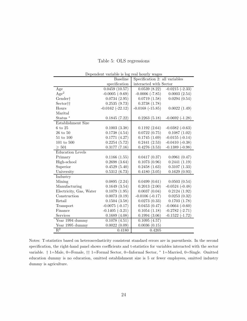
Table 5: OLS regressions
Dependent variable is log real hourly wagesBaseline Specification 2: all variables
specification interacted with SectorAge 0.0459 (10.57) 0.0539 (8.22) -0.0215 (-2.33)Age2 -0.0005 (-9.69) -0.0006 (-7.85) 0.0003 (2.54)Gender† 0.0734 (2.95) 0.0719 (1.58) 0.0294 (0.54)Sector†† 0.2535 (9.73) 0.3738 (1.78)Hours -0.0162 (-22.12) -0.0168 (-15.85) 0.0022 (1.49)MaritalStatus ∗ 0.1845 (7.22) 0.2263 (5.18) -0.0692 (-1.28)Establishment Size6 to 25 0.1003 (3.38) 0.1192 (2.64) -0.0382 (-0.63)26 to 50 0.1738 (4.54) 0.0722 (0.75) 0.1087 (1.02)51 to 100 0.1771 (4.27) 0.1745 (1.69) -0.0155 (-0.14)101 to 500 0.2254 (5.72) 0.2441 (2.53) -0.0410 (-0.38)≥ 501 0.3177 (7.16) 0.4276 (3.53) -0.1389 (-0.98)Education LevelsPrimary 0.1166 (1.55) 0.0417 (0.37) 0.0961 (0.47)High-school 0.2698 (3.64) 0.1073 (0.96) 0.2441 (1.19)Superior 0.4529 (5.40) 0.2458 (1.63) 0.3107 (1.33)University 0.5312 (6.73) 0.4180 (3.05) 0.1629 (0.93)IndustryMining 0.0895 (2.24) 0.0499 (0.61) 0.0503 (0.54)Manufacturing 0.1649 (3.54) 0.2013 (2.00) -0.0524 (-0.48)Electricity, Gas, Water 0.1079 (1.95) 0.0037 (0.04) 0.2124 (1.92)Construction 0.0073 (0.19) -0.0106 (-0.17) 0.0253 (0.32)Retail 0.1504 (3.58) 0.0273 (0.33) 0.1703 (1.78)Transport -0.0075 (-0.17) 0.0453 (0.47) -0.0664 (-0.60)Finance -0.1405 (-3.21) 0.1054 (1.18) -0.2782 (-2.71)Services 0.1689 (4.08) 0.1994 (3.06) -0.1522 (-1.72)Year 1994 dummy 0.1078 (4.51) 0.1095 (4.57)Year 1995 dummy 0.0022 (0.09) 0.0036 (0.15)R2 0.4180 0.4205
Notes: T-statistics based on heteroscedasticity consistent standard errors are in parenthesis. In the secondspecification, the right-hand panel shows coefficients and t-statistics for variables interacted with the sectorvariable. † 1=Male, 0=Female, †† 1=Formal Sector, 0=Informal Sector, ∗ 1=Married, 0=Single. Omittededucation dummy is no education, omitted establishment size is 5 or fewer employees, omitted industrydummy is agriculture.
24

Table 6: OLS regressions with two-step correction for selection bias
Dependent variable is log real hourly wages
Formal sector Informal sectorAge 0.0348 (6.05) 0.0553 (8.32)Age2 -0.0004 (-5.06) -0.0007 (-7.98)Gender 0.1240 (4.18) 0.0795 (1.55)Hours -0.0145 (-14.27) -0.0170 (-16.01)MaritalStatus 0.1715 (5.47) 0.2251 (4.84)Establishment Size6 to 25 emp. 0.0860 (2.15) 0.1198 (2.66)26 to 50 0.1872 (4.24) 0.0641 (0.66)51 to 100 0.1630 (3.36) 0.1672 (1.62)101 to 500 0.2064 (4.40) 0.2461 (2.54)≥ 501 0.2950 (5.73) 0.4244 (3.62)Education LevelsPrimary 0.2895 (2.83) 0.0761 (0.65)High-school 0.5341 (5.29) 0.1483 (1.19)Superior 0.7730 (7.05) 0.2970 (1.59)University 0.7829 (7.30) 0.4691 (3.16)IndustryMining 0.1031 (2.25) 0.0560 (0.69)Manufacturing 0.1489 (2.83) 0.1975 (2.08)Electricity, Gas, Water 0.2147 (3.15) 0.0101 (0.12)Construction 0.0172 (0.37) -0.0058 (-0.19)Retail 0.1961 (4.07) 0.0368 (0.45)Transport -0.0217 (-0.42) 0.0487 (0.50)Finance -0.1695 (-3.34) 0.1092 (1.22)Services 0.0499 (0.84) 0.2078 (3.19)Year 1994 dummy 0.1397 (4.78) 0.0623 (1.52)Year 1995 dummy 0.0669 (2.22) -0.1048 (-2.46)ρ 0.1020 (5.25) 0.0047 (0.03)
Notes: T-statistics are in parenthesis. The selection equation is: Prob(Sector = 1) = −1.3809+ .0163Age+.3576Gender + .2448Mstatus + .3433Primary + .7656Highschool + 1.4240Superior + 1.1179University +.3115Fhousehold, where Fhousehold = 1 if the worker has a formally employed family member, 0 otherwise.All variables in the selection equation are significant at the 1% level. The last row of the table gives theestimated correlation between the error term of the selection equation and the error term of the wageequation. Omitted variables are the same as in table 5.
25

Table 7: Results of Probit estimation of propensity scores
1993 1994 1995Age 0.0135 (0.0016) 0.0134 (0.0016) 0.0151 (0.0016)Gender 0.2161 (0.0438) 0.1249 (0.0442) 0.2013 (0.0440)FHousehold 0.2520 (0.0425) 0.2200 (0.0423) 0.2296 (0.0441)Establishment Size6 to 25 0.9601 (0.0513) 0.7920 (0.0502) 0.9323 (0.0510)26 to 50 1.4489 (0.0718) 1.3663 (0.0728) 1.6582 (0.0843)51 to 100 1.4243 (0.0790) 1.3771 (0.0803) 1.6925 (0.0878)101 to 500 1.6716 (0.0758) 1.6826 (0.0812) 1.6865 (0.0753)≥ 501 1.8223 (0.0911) 1.7141 (0.0951) 1.7771 (0.0998)EducationPrimary -1.5025 (0.0819) -1.2957 (0.0810) -1.3796 (0.0823)High-school -1.2181 (0.0757) -0.9549 (0.0731) -1.1825 (0.0761)Superior -1.0624 (0.1144) -0.4620 (0.1165) -0.7888 (0.1184)University -1.0896 (0.0884) -0.8732 (0.0879) -1.1351 (0.0872)
Notes: The dependent variable is 1 if the individual is in the formal sector. The High-school dummy includesnormal, technical and commercial high school education. Omitted education dummy is no education, omittedestablishment size is 5 or fewer employees. Asymptotic standard errors are in parentheses.
Table 8: Frequency distribution of propensity scores
1993 1994 1995P (Sector = 1|X, Y ) Formal Informal Formal Informal Formal Informal0.00 to 0.20 0.016 0.166 0.003 0.071 0.007 0.0880.20 to 0.40 0.097 0.401 0.108 0.437 0.113 0.4760.40 to 0.60 0.082 0.127 0.095 0.166 0.060 0.1270.60 to 0.80 0.293 0.192 0.246 0.199 0.234 0.1710.80 to 1.00 0.513 0.115 0.549 0.126 0.586 0.137
26

Table 9: Individual and establishment characteristics, 0.0 < P (Sector = 1|X, Y ) ≤ 0.2
1993 1994 1995Formal Informal Formal Informal Formal Informal
EducationNone 0.00 0.00 0.00 0.00 0.00 0.00Primary 0.80 0.85 1.00 1.00 0.64 0.76High-school 0.20 0.15 0.00 0.00 0.23 0.11Superior 0.00 0.00 0.00 0.00 0.00 0.00University 0.00 0.00 0.00 0.00 0.14 0.13Establishment size (employees)5 or fewer 1.00 1.00 1.00 1.00 1.00 1.006 to 25 0.00 0.00 0.00 0.00 0.00 0.0026 to 50 0.00 0.00 0.00 0.00 0.00 0.0051 to 100 0.00 0.00 0.00 0.00 0.00 0.00101 to 500 0.00 0.00 0.00 0.00 0.00 0.00More than 501 0.00 0.00 0.00 0.00 0.00 0.00GenderMale 0.47 0.33 0.67 0.37 0.05 0.29Female 0.53 0.67 0.33 0.63 0.95 0.71Another family member in the formal sectorYes 0.12 0.12 0.00 0.16 0.00 0.05No 0.88 0.88 1.00 0.84 1.00 0.95Average age 27.04 26.37 20.22 21.42 22.86 20.66Observations 51 332 9 132 22 160
27

Table 10: Individual and establishment characteristics, 0.2 < P (Sector = 1|X, Y ) ≤ 0.4
1993 1994 1995Formal Informal Formal Informal Formal Informal
EducationNone 0.00 0.00 0.00 0.00 0.00 0.00Primary 0.40 0.41 0.46 0.52 0.45 0.52High-school 0.45 0.46 0.46 0.42 0.42 0.39Superior 0.03 0.03 0.00 0.00 0.01 0.02University 0.12 0.11 0.07 0.06 0.12 0.08Establishment size (employees)5 or fewer 1.00 0.99 1.00 1.00 1.00 1.006 to 25 0.00 0.01 0.00 0.00 0.00 0.0026 to 50 0.00 0.00 0.00 0.00 0.00 0.0051 to 100 0.00 0.00 0.00 0.00 0.00 0.00101 to 500 0.00 0.00 0.00 0.00 0.00 0.00More than 501 0.00 0.00 0.00 0.00 0.00 0.00GenderMale 0.68 0.49 0.63 0.48 0.59 0.48Female 0.32 0.51 0.37 0.52 0.41 0.52Another family member in the formal sectorYes 0.42 0.43 0.40 0.39 0.39 0.37No 0.58 0.57 0.60 0.61 0.61 0.63Average age 35.99 35.68 34.35 33.12 35.65 33.21Observations 315 805 367 811 378 868
28

Table 11: Individual and establishment characteristics, 0.4 < P (Sector = 1|X, Y ) ≤ 0.6
1993 1994 1995Formal Informal Formal Informal Formal Informal
EducationNone 0.00 0.00 0.00 0.00 0.00 0.00Primary 0.60 0.63 0.60 0.49 0.46 0.46High-school 0.28 0.28 0.28 0.36 0.39 0.41Superior 0.04 0.03 0.05 0.07 0.05 0.05University 0.09 0.05 0.08 0.08 0.11 0.08Establishment size (employees)5 or fewer 0.16 0.18 0.35 0.41 0.34 0.406 to 25 0.83 0.82 0.65 0.59 0.66 0.6026 to 50 0.00 0.00 0.00 0.00 0.00 0.0051 to 100 0.01 0.00 0.00 0.00 0.00 0.00101 to 500 0.00 0.00 0.00 0.00 0.00 0.00More than 501 0.00 0.00 0.00 0.00 0.00 0.00GenderMale 0.61 0.65 0.71 0.60 0.51 0.57Female 0.39 0.35 0.29 0.40 0.49 0.43Another family member in the formal sectorYes 0.25 0.30 0.33 0.36 0.30 0.29No 0.75 0.70 0.67 0.64 0.70 0.71Average age 33.43 31.08 36.53 34.65 35.00 35.88Observations 268 254 322 308 199 232
29
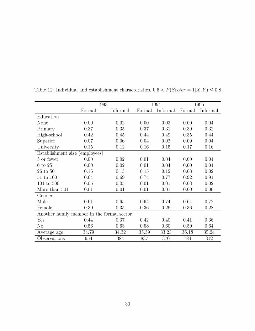
Table 12: Individual and establishment characteristics, 0.6 < P (Sector = 1|X, Y ) ≤ 0.8
1993 1994 1995Formal Informal Formal Informal Formal Informal
EducationNone 0.00 0.02 0.00 0.03 0.00 0.04Primary 0.37 0.35 0.37 0.31 0.39 0.32High-school 0.42 0.45 0.44 0.49 0.35 0.44Superior 0.07 0.06 0.04 0.02 0.09 0.04University 0.15 0.12 0.16 0.15 0.17 0.16Establishment size (employees)5 or fewer 0.00 0.02 0.01 0.04 0.00 0.046 to 25 0.00 0.02 0.01 0.04 0.00 0.0426 to 50 0.15 0.13 0.15 0.12 0.03 0.0251 to 100 0.64 0.69 0.74 0.77 0.92 0.91101 to 500 0.05 0.05 0.01 0.01 0.03 0.02More than 501 0.01 0.01 0.01 0.01 0.00 0.00GenderMale 0.61 0.65 0.64 0.74 0.64 0.72Female 0.39 0.35 0.36 0.26 0.36 0.28Another family member in the formal sectorYes 0.44 0.37 0.42 0.40 0.41 0.36No 0.56 0.63 0.58 0.60 0.59 0.64Average age 34.79 34.32 35.39 33.23 36.18 35.24Observations 954 384 837 370 784 312
30

Table 13: Individual and establishment characteristics, 0.8 < P (Sector = 1|X, Y ) ≤ 1.0
1993 1994 1995Formal Informal Formal Informal Formal Informal
EducationNone 0.01 0.02 0.01 0.04 0.00 0.02Primary 0.20 0.20 0.20 0.27 0.26 0.28High-school 0.43 0.40 0.42 0.38 0.38 0.31Superior 0.08 0.10 0.13 0.08 0.11 0.10University 0.27 0.28 0.25 0.24 0.25 0.30Establishment size (employees)5 or fewer 0.00 0.01 0.00 0.02 0.00 0.016 to 25 0.03 0.05 0.06 0.08 0.03 0.1026 to 50 0.22 0.27 0.20 0.24 0.23 0.2351 to 100 0.15 0.20 0.21 0.22 0.22 0.22101 to 500 0.33 0.28 0.30 0.25 0.31 0.30More than 501 0.27 0.19 0.24 0.18 0.21 0.14GenderMale 0.69 0.75 0.64 0.71 0.65 0.60Female 0.31 0.25 0.36 0.29 0.35 0.40Another family member in the formal sectorYes 0.55 0.49 0.52 0.47 0.49 0.46No 0.45 0.51 0.48 0.53 0.51 0.54Average age 40.16 38.58 38.76 40.01 38.52 36.64Observations 1673 230 1871 234 1961 250
31

Table 14: Matching estimators
Period calliper Nearest neighbor1993 -0.084 (0.075) 0.052 (0.081)1994 -0.183 (0.072) 0.110 (0.075)1995 -0.168 (0.079) 0.022 (0.088)
Notes: In Calliper matching, δ = 10−4. Standard errors are in parenthesis.
Table 15: Calliper matching estimator for various subgroups
1993 1994 1995αM Std. error αM Std. error αM Std. error
P (Sector = 1|X, Y ) ∈ [0.0, 0.2] -0.523 0.345 -0.389 0.370 -1.415 0.505P (Sector = 1|X, Y ) ∈ (0.2, 0.4] -0.291 0.149 -0.452 0.135 -0.443 0.136P (Sector = 1|X, Y ) ∈ (0.4, 0.6] -0.338 0.149 -0.254 0.198 0.045 0.246P (Sector = 1|X, Y ) ∈ (0.6, 0.8] -0.222 0.136 -0.045 0.131 -0.156 0.146P (Sector = 1|X, Y ) ∈ (0.8, 1.0] 0.369 0.174 -0.092 0.145 -0.045 0.144Females -0.064 0.094 -0.181 0.089 -0.150 0.095Males -0.116 0.098 -0.137 0.091 -0.043 0.108Age ≤ 40 -0.055 0.126 -0.282 0.129 -0.360 0.112Low education -0.228 0.115 -0.298 0.102 -0.077 0.110Large establishments 0.444 0.214 0.005 0.221 -0.087 0.167
Notes: Low education individuals have some primary education or less.
Table 16: Calliper matching estimator without controlling for establishment size
1993 1994 1995αM Std. error αM Std. error αM Std. error
Full sample 0.240 0.049 0.228 0.044 0.212 0.044Age ≤ 40 0.312 0.048 0.228 0.040 0.226 0.042Females 0.172 0.068 0.111 0.060 0.115 0.062Males 0.275 0.049 0.259 0.044 0.262 0.044Low education 0.083 0.049 0.107 0.042 0.099 0.042
32

Table 17: Sample transitions
Period Movers Stayers5-1993 to 10-1993 116 20510-1993 to 5-1994 103 2065-1994 to 10-1994 104 22110-1994 to 5-1995 63 1705-1995 to 10-1995 73 230
Table 18: Difference-in-difference Calliper matching estimator, δ = 10−3
Period αMDD Std. error5-1993 to 10-1993 -0.506 0.45210-1993 to 5-1994 -0.708 0.3615-1994 to 10-1994 -0.639 0.29510-1994 to 5-1995 -0.221 0.3025-1995 to 10-1995 0.436 0.526
Notes: We use a lower value of δ because of the reduced number of observations.
Table 19: Difference-in-difference Calliper matching estimator for subgroups
Period Males Females Low education Age ≤ 405-1993 to 10-1993 0.253 (0.543) -1.305 (0.732) -1.036 (0.907) -0.1419 (0.518)10-1993 to 5-1994 0.165 (0.536) -0.165 (0.536) -1.664 (0.437) -1.348 (0.429)5-1994 to 10-1994 -0.437 (0.335) -0.666 (0.781) -0.234 (0.318) -0.725 (0.328)10-1994 to 5-1995 0.589 (0.515) -1.253 (0.318) -0.491 (0.227) 0.158 (0.367)5-1995 to 10-1995 0.250 (0.719) 1.234 (1.333) 1.010 (0.745) 0.496 (0.719)
Notes: Standard errors in parenthesis. Age ≤ 40 refers to individuals below 40 years of age at the end of theperiod.
33

Table 20: Matching estimators for measures of job satisfaction
1993 1994 1995Are you looking for another job?Full sample 0.012 (0.030) -0.041 (0.031) -0.069 (0.034)Men -0.012 (0.038) -0.048 (0.038) -0.042 (0.044)Women 0.063 (0.051) -0.084 (0.057) -0.147 (0.049)Age ≤ 40 0.010 (0.039) -0.065 (0.041) -0.066 (0.042)Primary orless education 0.011 (0.053) -0.021 (0.050) -0.074 (0.053)Large establishments -0.036 (0.051) -0.036 (0.060) -0.138 (0.070)Would you like to work more hours?Full sample -0.016 (0.021) -0.059 (0.022) -0.097 (0.023)Men -0.023 (0.025) -0.044 (0.026) -0.033 (0.030)Women -0.036 (0.038) -0.136 (0.042) -0.237 (0.038)Age ≤ 40 -0.023 (0.025) -0.047 (0.028) -0.081 (0.028)Primary orless education -0.048 (0.034) -0.011 (0.035) -0.052 (0.038)Large establishments 0.187 (0.061) 0.083 (0.063) -0.078 (0.063)How many hours do you work a week in your primary occupation?Full sample -0.061 (0.027) -0.014 (0.031) -0.033 (0.035)Men -0.021 (0.027) -0.045 (0.031) -0.082 (0.035)Women -0.108 (0.059) 0.093 (0.070) 0.109 (0.062)Age ≤ 40 -0.088 (0.035) -0.004 (0.042) -0.079 (0.042)Primary orless education 0.005 (0.051) -0.015 (0.056) 0.013 (0.061)Large establishments -0.048 (0.053) 0.013 (0.052) 0.114 (0.075)
Notes: Entries are calliper matching estimators for answers to the questions in italics. In bottom panel, wecompare log(hours worked) in the two sectors. Standard errors are in parenthesis.
34

References
Blundell, R., Costa Diaz, M., “Evaluation Methods for Non Experimental Data,” FiscalStudies 21 (2000): 427-468.
Blundell, R., Costa Diaz, M., Meghir, C. and Van Reenan, J., “Evaluating the EmploymentImpact of Mandatory Job-search Assistance: the UK New Deal Gateway,” Institute ofFiscal Studies manuscript (2000).
Dehejia, R.H, and Wahba, S., “Causal Effects in Non Experimental Studies: Re-evaluatingthe Evaluation of Training Programs,” Journal of the American Statistical Association94 (1999): 1053-1062.
Dehejia, R.H, and Wahba, S., “Propensity Score Matching Methods for Non ExperimentalCausal Studies”, Review of Economics and Statistics (forthcoming).
Fields, G. S., “Rural-Urban Migration, Urban Unemployment and Under-Development, andJob-Search Security in LDCs,” Journal of Development Economics 2 (1975): 165-87.
Fortin, B., Marceau, N. and Savard, L., “Taxation, Wage Controls and the Informal Sector,”Journal of Public Economics 66 (1997): 239-312.
Gong, X. and Van Soest, A., “Wage Differentials and Mobility in the Urban Labor Market:A Panel Data Analysis for Mexico”, IZA, Bonn discussion paper No. 329 (2001).
Harris, J. R. and Todaro, M. P., “Migration, Unemployment and Development: A Two-Sector Analysis,” American Economic Review 60 (1970): 126-142.
Heckman, J. J., Ichimura, H., Smith, J., and Todd, P., “Characterizing Selection Bias UsingExperimental Data,” Econometrica 66 (1998): 1017-1098.
Heckman, J. J., Ichimura, H, and Todd, P.E., 1“Matching as an Econometric EvaluationEstimator: Evidence from Evaluating a Job Training Program,” Review of EconomicStudies 64 (1997): 605-654.
Heckman, J. J., and Hotz, V., “An investigation of Labor Market Earnings of PanamanianMales”, Journal of Human Resources, 21 (1986): 507-542.
Heckman, J. J., Lalonde, R. and Smith, J., “The Economics and Econometrics of ActiveLabor Market Programs”, in O. Ashenfelter and D. Card (eds), Handbook of LaborEconomics, v3 (1999).
Lalonde, R., “Evaluating the Econometric Evaluations of Training Programs,” AmericanEconomic Review 76 (1986): 604-620.
Lewis, W. A., “Economic Development with Unlimited Supplies of Labour,” ManchesterSchool 22 (1954): 139-191.
35

Loayza, N.V., “The Economics of the Informal Sector: A Simple Model and Some EmpiricalEvidence from Latin America,” Carnegie-Rochester Conference Series on Public Policy45 (1996): 129-162.
Maloney, W. F., “Does Informality Imply Segmentation in Urban Labor Markets? Evidencefrom Sectoral Transitions in Mexico,” The World Bank Economic Review 13 (1999):275-302.
Magnac, Th., “Segmented or Competitive Labor Markets,” Econometrica 59 (1991): 165-187.
Mazumdar, D., “The Theory of Urban Employment in Less Developed Countries,”WorldDevelopment 4 (1975): 655-679.
Mazumdar, D., “The Urban Labor Market Income Distribution: A Study of Malaysia”(Oxford University Press, 1981).
Oi, W. Y., Idson, T. L., “Firm Size and Wages,” in Ashenfelter, O. C., Card, D. (eds),Handbook of Labor Economics, v3b (1999).
Persson, T., Tabellini, G and Trebbi, F., “Electoral Rules and Corruption,” IEES manu-script (2000).
Portes, A., Castells, M., and Benton, L.A., (eds.), “The Informal Economy: Studies in Ad-vanced and Less Developed Countries,” (Baltimore: Johns Hopkins University Press,1989).
Pradhan, M. and Van Soest, A., “Formal and Informal Sector Employment in Urban Areasof Bolivia,” Labor Economics 2 (1995): 275-297.
Rauch, J.E., “Modeling the Informal Sector Formally,” Journal of Development Economics35 (1991): 33-48.
Roberts, B.R., “Employment Structure, Life Cycle, and Life Chances: Formal and InformalSectors in Guadalajara,” in Portes, A., Castells, M., and Benton, L.A. (eds.), TheInformal Economy: Studies in Advanced and Less Developed Countries, (Baltimore:Johns Hopkins University Press, 1989).
Rosenbaum, P. and Rubin, D.B., “The Central Role of the Propensity Score in Observa-tional Studies for Causal Effects,” Biometrika 70 (1983): 41-55.
Rosenbaum, P. and Rubin, D.B., “Reducing Bias in Observational Studies using Sub Clas-sification on the Propensity Score,” Journal of the American Statistical Association 79(1984): 516-524.
Sarte, P.G., “Informality and Rent-Seeking Bureaucracies in a Model of Long-Run Growth,”Journal of Monetary Economics 46(2000): 173-97.
36

Smith, J. and Todd, P., “Reconciling Conflicting Evidence on the Performance of Propensity-Score Matching Methods”, American Economic Review 91 (2001): 112-18.
Tansel, A., “Formal versus Informal Sector Choice of Wage Earners and Their Wages inTurkey,” Economic Research Forum Working Paper No. 9927 (1999).
37