are real options “real”? isolating uncertainty from risk
TRANSCRIPT

Munich Personal RePEc Archive
Are Real Options “Real”? Isolating
Uncertainty from Risk in Real Options
Analysis
So, Leh-chyan
National Tsing Hua University
2013
Online at https://mpra.ub.uni-muenchen.de/52493/
MPRA Paper No. 52493, posted 26 Dec 2013 15:13 UTC
Are Real Options “Real”?
Isolating Uncertainty from Risk in Real Options Analysis*
Leh-chyan So Department of Quantitative Finance
National Tsing Hua University
Taiwan
Revised: November 2013
* The author would like to thank participants at the 15th Annual International Conference on Real Options in Turku, Finland for useful comments and suggestions. The author is grateful for the helpful comments and suggestions of a reviewer.

1
Abstract
This paper derives an adjusted Black-Scholes pricing formula. In separating risk
and uncertainty using the robust control technique, we find that both uncertainty and
risk raise management’s subjective evaluation of real options. We suggest a simple
method to filter the risk of the project and to acquire a more reliable value of real
options without the influence of uncertainty. In addition, we propose that an
investment opportunity may be postponed inappropriately, as under uncertainty the
exercise of investment may be delayed by the project manager. To our knowledge, any
similar quantitative methods have not hitherto been mentioned in terms of isolating
uncertainty from risk in real options analysis that we consider here.
Keywords: Option to defer, investment opportunity, uncertainty, Black-Scholes
pricing formula, volatility.
JEL: G11, G12, G13.

2
1. Introduction
Many approaches have proposed methods to evaluate investment opportunities.
Among them, traditional discounted cash flow (DCF) approaches, such as the
standard net present value (NPV), are easy to apply but have been criticized for their
neglect of a project manager’s flexibility to adjust earlier decisions according to
uncertainties that are revealed later (for example, Trigeorgis, 1996). On the contrary,
real options have enjoyed great popularity recently (for example, Dixit and Pindyck,
1994; Trigeorgis, 1996; Amram and Kulatilaka, 1999) since, in the real world,
managers have the right to undertake investment opportunities and realize positive
profits. This flexibility not only protects managers against downside risk but also
provides upside potential.
As a manager has the flexibility to retract initial planning, it is risk and
uncertainty in the future that triggers an upgrade in the investment opportunity. Hence,
in the light of real options, the investment opportunity should be worth more when its
volatility is high. Real options extend financial options into an investment opportunity
analysis of real assets and often assign a higher value to the investment opportunity
because of the value of time.
In practice, the Black-Scholes pricing formula is commonly used in real options
analysis. Many studies have reported the influence and estimation of the six factors
affecting the price of an option (for example, Leslie and Michaels, 1997; Davis, 1998;
Fernandez, 2013). Among the six key factors, volatility is especially notorious for the
difficulty in estimation (for example, Lander and Pinches, 1998). Furthermore, option
prices are very sensitive to estimation of the volatility of the underlying assets. As
noted in Trigeorgis (1990), a 50 percent increase in volatility raises the option value
by about 40 percent.
In the Black-Scholes model, volatility, , is defined as the standard deviation of
the continuously compounded rate of return provided by the underlying asset within a
year. The binomial tree valuation approach proposed by Cox, Ross, and Rubinstein
(CRR, 1979), which also enjoys great popularity, preserves the notation and definition
of to depict future price movements. When we use the Black-Scholes model or
the CRR model, we have to use historical data to estimate the value of and
substitute it into the valuation model to find an option price.

3
If a project manager knows the true distribution process governing future price
movements, then there is less uncertainty. However, in most cases, during real options
analysis, the manager relies on imperfect knowledge of the model and parameters to
make decisions. For example, to highlight the importance of uncertainty in real
options analysis, Bräutigam, Esche, and Mehler-Bicher (2003) particularized nearly
every kind of uncertainty, such as project uncertainty, uncertainty about intangibles,
financial uncertainty, product uncertainty, market uncertainty, region-specific
uncertainty, and unknown uncertainties, which shows how much uncertainty can be
present.
One simple way of dealing with uncertainty is to raise the original volatility
slightly, which has been estimated to show that future price movement could be more
volatile due to uncertainty arising from personal judgment. The idea behind this rule
of thumb is that risk and uncertainty share reasonably similar meanings, and they are
used interchangeably in many cases.
Although the terms risk and uncertainty are often used interchangeably in the
literature in links to volatility, they have different meanings. Risk, an objective term,
represents a probability distribution of potential outcomes. Risk aversion is an attitude
that penalizes the expected return of a risky investment. Consider the following
situation. An investment pays off either $1 or $0 with equal probability. Another pays
off $0.5 with certainty. Although the two investments offer the same expected return,
a risk-averse investor will reject the investment in the former.
Uncertainty is a subjective term and represents a lack of confidence in
probability estimates. If people are uncertain, they worry about a worst-case scenario.
The following example is adapted from Ellsberg’s (1961) experiment. There are two
urns, each of which contains several red and green balls. The total number of the balls
in each urn is the same. The balls in one urn are half red and half green. However, the
ratio in the other urn is unknown to the player. The rule is that $1 can be obtained
when a red ball is drawn out. Although the two urns offer the same expected return, an
uncertainty-averse investor will not draw a ball from the latter because the investor
tends to think pessimistically, and so expects that the urn offers lower odds.
Recent studies have found that risk and uncertainty have different influences on
decision makers. Alessandri’s (2003) empirical findings show that managers treat risk
and uncertainty separately, and use different decision rules to respond to each.
Alessandri et al. (2004) emphasize the importance of identifying the risks and

4
uncertainties inherent in the decision-making process. They suggested that qualitative
approaches should be used instead of quantitative ones to evaluate capital projects
with higher uncertainty.
Nishimura and Ozaki (2006) showed that uncertainty and risk have different
effects on the value of an investment opportunity. Miao and Wang (2011) emphasized
the effect of distinguishing risk from uncertainty for an option exercise or in the
optimal exit problem. Trojanowska and Kort (2010) focused on how uncertainty
affects investment timing. They claimed that uncertainty aversion causes a firm to
consider a project to have higher risk and to overprice the risk when there is
uncertainty. They predicted that the probability of investment monotonically decreases
according to the level of uncertainty in long-term projects. By using the
Choquet-Brownian motions to describe uncertainty, Roubaud, Lapied, and Kast (2010)
suggested that a decision maker’s pro and con attitudes toward ambiguity might
influence the decision to exercise options to invest.
Owing to the above arguments, it is possible that such a rule of thumb offers
room for the manager to manipulate the parameter, , in the Black-Scholes pricing
formula to exaggerate the value of an investment opportunity. Should we not consider
risk purely in the uncertainty-absent Black-Scholes world if we are unanimous
regarding the objectivity of the Black-Scholes model?
The purpose of this paper is to separate uncertainty from risk in the commonly
used Black-Scholes pricing formula and to examine how uncertainty affects option
prices. We show that the value of real options obtained by the Black-Scholes pricing
formula may not be real if the concepts of risk and uncertainty are vague. In addition,
we want to show that uncertainty can affect the timing of investments.
First, we describe the basic framework. The approach is most closely associated
with the robust control approach to uncertainty, which depicts model uncertainty
through a set of priors and introduces a penalty function to a general utility function in
order to capture investor uncertainty (for example, Anderson, Hansen, and Sargent,
2000; Kogan and Wang, 2002; Boyle, Uppal, and Wang, 2003; Uppal and Wang, 2003;
Maenhout, 2004). Investors under high uncertainty are concerned about a worst-case
scenario. Consequently, the investor will choose alternative models that are distant
from the reference model. Hence, the robust control approach assigns a lower penalty
to distant perturbations. If the level of uncertainty is low, the investor will choose
alternative models that are similar to the reference model. Hence, the robust control

5
approach assigns a higher penalty to more distant perturbations. The penalty is
inversely relative to the investor’s uncertainty.
The organization of the remainder of the paper is as follows. The model and
theoretical results are described in Section 2, a numerical example is given in Section
3, and the conclusions are presented in the final section.
2. Model
2.1 Basic concepts
We have already shown that risk and uncertainty have different influences on
decision makers and on the value of an investment opportunity. However, according
to the definition of the original Black-Scholes model, only risk is taken into
consideration when pricing contingent claims. By using the robust control technique,
we added an extra parameter to depict a decision maker’s attitude of uncertainty and
derived an adjusted Black-Scholes pricing formula. By denoting risk and uncertainty
as two parameters in the pricing formula, we can avoid the problem arising from using
these two terms interchangeably, and can assess their influences separately. As a result,
the evaluation of real options, as well as the optimal investment timing, may be more
reliable.
2.2 Theoretical model
Throughout the paper, we denote the risk-free interest rate by a constant, r . We
assume that the gross project value, S , follows the geometric Brownian motion with
expected return, , and volatility, :
.dBdtS
dS (1)
Taking the non-traded property of the underlying asset, we assume that the
below-equilibrium return shortfall is q (for example, McDonald and Siegel, 1986).
Hence, the dynamic process of the gross project value is adjusted to:

6
.)( dBdtqS
dS (2)
In the literature, q functions as a dividend yield. The expected return of S with
dividend is v .
2.2.1 Decision process for the manager under no uncertainty
Suppose that the manager knows the true probability law of the project return,
given the probability measure Q . The total wealth dynamic process of the manager
is:
,))(( dBdtWCrvr
WdW (3)
where represents the proportion of wealth allocated to the investment project.
The expected utility of the manager in continuous time is:
,)( )(
T
t TtT
ssQ
t JedsCueEJ
where )( sCu takes the form of the power utility, )( sCu =
1
1sC , where is the risk
aversion coefficient.
Suppose that the manager has to choose optimal consumption and investment
weights to maximize utility:
.021)()(max 222
,
wwwtCJW
WCrvrWJJcu (4)
By taking derivatives of (4) with respect to C and , we have the optimal
consumption:

7
,Wc Ju (5)
and investment choice:
),(2 rvWJ
Jww
w
(6)
implied by the first-order conditions.
In order to derive the exact formula for the optimal investment in the project, we
have to specify the form of the value function. As it is assumed that the manager has
power utility
1)(
1s
sC
Cu , the value function takes the form:
1)(
1WWJ , (7)
where is a constant depending on the parameter of the environment.
Substituting (7) into (6), the optimal portfolio weight in the investment
opportunity for the manager is given by 2)(
rv .
2.2.2 Decision process for the manager under uncertainty
When the manager is under uncertainty and is not confident about the
probability estimates, we have to apply the robust control technique to deal with this
issue. Moreover, when the manager has to evaluate the investment opportunity using
real options analysis under uncertainty, the misspecification problem should be taken
into account.
Suppose that the manager considers the alternative model, Q , rather than the
reference model, Q . Applying Uppal and Wang’s (2003) method, the optimization
problem should be adjusted to:

8
(8) ,0
2)(
21)()(
infsup222
222
,
JWJ
JWWCrvrWJJCu
w
wwwt
C
where the second line of the brace is additional to (4), and the former term of the
second line reflects the adjusted drift term resulting from the change of measure from
Q to Q . The term reflects the difference between the adjusted drift term and
the original one. The latter term of the second line is associated with the penalty
function, where )(J converts the penalty to units of the utility. In addition, we use
, the penalty parameter, to measure the manager’s subjective confidence about the
reference model.
As mentioned above, the manager under uncertainty worries about a worst-case
scenario. The manager will then choose alternative models that are more distant from
the reference model. As a result, the robust control approach assigns a lower penalty
to more distant perturbations. If the level of uncertainty is low, the investor will
choose alternative models that are much the same as the reference model. As a result,
the robust control approach assigns a higher penalty to more distant perturbations.
That is, the lower is the value of , the higher is the level of the manager’s
uncertainty, and the penalty is inversely related to the investor’s uncertainty. Hence,
the reciprocal of can be treated as the level of the manager’s uncertainty. We have
used a similar framework with an extension of inserting multi-dimensional Lagrange
multipliers to discuss issues on evaluation of employee stock options in So (2009),
where the techniques to solve this kind of optimization problem are given in greater
detail.
The optimal consumption can be obtained by solving the first-order condition
.Wc Ju After taking derivatives of (8) with respect to , we obtain:
.)(2ww
w
ww
w
WJJrv
WJJ
(9)
Differentiating (8) with respect to , we obtain:
9
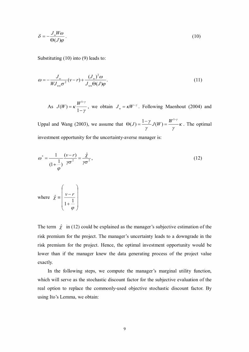
)(J
WJw
. (10)
Substituting (10) into (9) leads to:
.)(
)()(2
2
JJJrv
WJJ
ww
w
ww
w
(11)
As
1)(
1WWJ , we obtain WJw . Following Maenhout (2004) and
Uppal and Wang (2003), we assume that
1
)(1)( WWJJ . The optimal
investment opportunity for the uncertainty-averse manager is:
,ˆ)(
)11(
122
*
rv (12)
where
11
ˆ rv
The term ̂ in (12) could be explained as the manager’s subjective estimation of the
risk premium for the project. The manager’s uncertainty leads to a downgrade in the
risk premium for the project. Hence, the optimal investment opportunity would be
lower than if the manager knew the data generating process of the project value
exactly.
In the following steps, we compute the manager’s marginal utility function,
which will serve as the stochastic discount factor for the subjective evaluation of the
real option to replace the commonly-used objective stochastic discount factor. By
using Ito’s Lemma, we obtain:

10
(13) ,)(
))(1(21)()()(
)()1)((21
)()()(
)()1)((21
)()()(
)(21
*
22**
*22**
22*
**
*22**
22*22
**
*22**1
22
2
dBW
dtWCrvrW
dtW
dBdtWCrvrW
dtWW
dBWdtWCrvrWW
dWWJdW
WJdt
tJdJ www
w
where dB is a Brownian motion under the new measure Q .
By using
1)(
1WWJ , we can show that
WJw , (14)
and substitution of (14) into (13) leads to:
.)(
))(1(21)()(
*
22**
*2**
dBJ
dtWCrvrJdJ
w
ww
(15)
Using (15), the dynamic process of the manager’s marginal utility function is
given by:
.
))(1(21)()(
*
22**
*2**
dB
dtWCrvr
JdJ
w
w
(16)
As Wc Ju is implied by the first-order condition, we have , WJCu wc

11
so that:
.1*
WC (17)
Substituting (17) into (16) leads to:
dB
dtrvrJ
dJw
w
*
22*1
*2**
))(1(21)()(
(18)
We need to arrange the terms in the brace of (18). Using
1)(
1WWJ and
substituting the optimal values into (8), we have the following relationship:
(19) .0)(2
)(
)()(21)()(
22**2*1
22*1*1**
JW
WrvrWCWCu
Combined with (17), (19) becomes
)20(.0)()1(2
)()1(
))()(1(21)()1(
1
22**2*
22**1
WJ
rvr
From (20), we obtain a simplified form of (18):
.)()1(
2)(
)()(*
1
2**2*
22**
dBdt
WJ
rvr
JdJ
w
w
(21)

12
Substituting
1
)(1)( WWJJ
and
)(J
WJw into (21),
we have:
.)(2
)21()( *22**
dBdtrvrJ
dJw
w
(22)
Finally, when we substitute (12) into (22), we can derive the dynamic process of
the manager’s subjective stochastic discount factor under uncertainty:
,)11(
)(ˆ)11(
)()1(2
)1()(22
2
dBrvdtrdBrvdtrvr
JdJ
w
w
(23)
where 22
2
)1(2)1()(ˆ
rvrr .
In the extreme case where approaches infinity, our result would be rr ˆ ,
which means that when the manager knows the true probability law of the project, the
subjective risk-free interest rate is exactly that of the real world. However, as the
manager here is risk-averse with 1 ,
rrvrr
22
2
)1(2)1()(ˆ
,
in general, implying that the manager’s uncertainty about the true probability law of
project returns may lead to the consideration that one dollar invested today has a
lower future value than its market value.
We explain the intuition behind this outcome. As the manager’s uncertainty
would lead to a downgrade in the risk premium for the investment opportunity, the
investment in the project shrinks. In other words, the manager over-invests in the
risk-free asset, providing a worse payoff than the investment opportunity. Owing to
this suboptimal allocation in the mind of the manager, one dollar invested today

13
provides a lower future value than its market value. This is the reason for observing
an inverse relationship between the subjective risk-free interest rate, r̂ , and the
subjective measure of confidence, .
2.2.3 Evaluation of real options for the manager under uncertainty
We derive the subjective value of the real option for the manager under
uncertainty. Let ),( tSR be the subjective price of the real option with the non-traded
asset as its underlying asset. Applying the martingale approach:
(24) 0.)(21
0),(),(),(
0)),((
2
dSRJ
dJJ
dJRdSRdtRdSREJ
tSdRdJdJtSRtSdRJE
tSRJdE
sw
w
w
wssts
Qw
wwwQ
wQ
Using (23), (24) can be rearranged as:
. 011
)(ˆ21)( 22
dtrvSRrRSRRqvSRJ ssstsw
(25)
As a result, the partial differential equation is given by:
(26) 0,ˆ)ˆˆ(21
011
)(ˆ21)(
22
22
tsss
sssts
RRrqrSRSR
rvSRrRSRRqvSR
where
22
2
)1(2)1()(ˆ
rvrr

14
and
111ˆˆ vrrqq .
When approaches infinity, rr ˆ , q̂ degenerates to q , and our result collapses
to the original Black-Scholes partial differential equation.
As we can consider equation (26) to be the typical Black-Scholes partial
differential equation with the subjective rate of return, r̂ , and the subjective
below-equilibrium return shortfall, q̂ , the subjective value of the real option on the
non-traded asset can be obtained immediately as:
),()(ˆ2
)(ˆ1
)(ˆ dNIedNSeC tTrtTq (27)
where I denotes that investment cost,
22
2
)1(2)1()(ˆ
rvrr ,
111ˆˆ vrrqq ,
tT
tTqrIS
d
))(2
ˆˆ()ln(2
1 , and tTdd 12 .
When approaches infinity, r̂ equals r and q̂ degenerates to q , which is
the result of the Black-Scholes pricing formula. However, when is more distant
from infinite, we have rr ˆ and qq ˆ . As the manager’s uncertainty decreases the
subjective below-equilibrium return shortfall more than it decreases the subjective
interest rate, the manager boosts the subjective value of the real option, compared
with the case where the manager is aware of the true probability law of project returns.
It can be argued that both uncertainty and risk have a positive effect on the value of
15
real options.
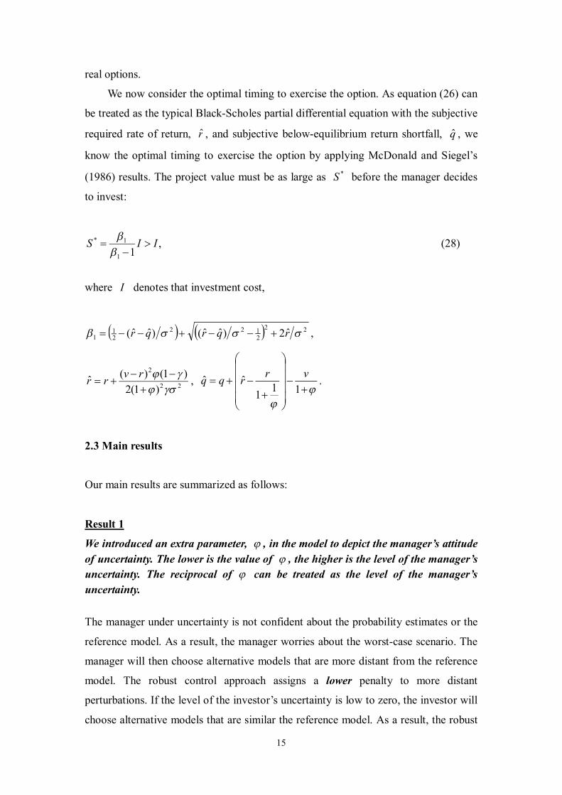
We now consider the optimal timing to exercise the option. As equation (26) can
be treated as the typical Black-Scholes partial differential equation with the subjective
required rate of return, r̂ , and subjective below-equilibrium return shortfall, q̂ , we
know the optimal timing to exercise the option by applying McDonald and Siegel’s
(1986) results. The project value must be as large as *S before the manager decides
to invest:
,11
1* IIS
(28)
where I denotes that investment cost,
222122
21
1 ˆ2)ˆˆ()ˆˆ( rqrqr ,
22
2
)1(2)1()(ˆ
rvrr ,
111ˆˆ vrrqq .
2.3 Main results
Our main results are summarized as follows:
Result 1
We introduced an extra parameter, , in the model to depict the manager’s attitude of uncertainty. The lower is the value of , the higher is the level of the manager’s uncertainty. The reciprocal of can be treated as the level of the manager’s uncertainty.
The manager under uncertainty is not confident about the probability estimates or the
reference model. As a result, the manager worries about the worst-case scenario. The
manager will then choose alternative models that are more distant from the reference
model. The robust control approach assigns a lower penalty to more distant
perturbations. If the level of the investor’s uncertainty is low to zero, the investor will
choose alternative models that are similar the reference model. As a result, the robust

16
control approach assigns a higher penalty to more distant perturbations. That is, the
lower is the value of , the higher is the level of the manager’s uncertainty.
Result 2
For the manager with power utility and with the attitude of uncertainty described in Result 1, the subjective value of the real option on the non-traded asset is
)()(ˆ2
)(ˆ1
)(ˆ dNIedNSeC tTrtTq , where I denotes that investment cost,
22
2
)1(2)1()(ˆ
rvrr ,
111ˆˆ vrrqq ,
tT
tTqrIS
d
))(2
ˆˆ()ln(2
1 ,
tTdd 12 , and the reciprocal of is the level of the manager’s uncertainty.
Result 3
The project value must be as large as *S before the manager with power utility and with the attitude of uncertainty described in Result 1 decides to invest:
IIS
11
1*
,
where I denotes the investment cost,
222122
21
1 ˆ2)ˆˆ()ˆˆ( rqrqr ,
22
2
)1(2)1()(ˆ
rvrr ,
111ˆˆ vrrqq ,
and the reciprocal of is the level of the manager’s uncertainty.
3. Numerical Example

17
Table 1 summarizes the values of all of the parameters used in calibration,
namely the risk aversion coefficient, ; the rate of return of the investment
opportunity, v ; the riskless interest rate, r ; the dividend yield (shortfall), q ; the
time to maturity, tT ; the volatility of the investment opportunity, ; and the
subjective measure of confidence about the probability law of project returns, .
Without further information, we assume that 04.0 qr (for example, Dixit
and Pindyck, 1994). In order to illustrate the effects of risk, we set volatility to lie in
the range (0.2, 0.5), that is, 20% to 50%. It is difficult to assign a value to the
subjective parameter, . However, Maenhout (2004) made a recommendation to
choose a suitable value of , namely should be chosen to make the difference
between the objective and subjective risk premium for the project less than 3% for a
95% confidence interval. We eliminate unreasonable values of less than 6, and let
the values of increase from 6 to infinity to examine how the subjective measure of
confidence about the probability law of the project return, or uncertainty, affects the
valuation of the real option.
Table 2 shows the values of real options after separating the effects of risk and
uncertainty. The results of neglect of uncertainty are shown in the column . We
find that the manager’s uncertainty, like risk, raises the subjective value of the real
options. Based on these findings, if we mistake uncertainty for risk and overestimate
the value of the parameter , we would conclude wrongly that the value of the real
option is high.
What is the more reliable value of the real option? We now provide a simple
method to filter the risk of the project and to acquire a more reliable value of real
options without the influence of uncertainty. As the Black-Scholes option pricing
formula does not take account of uncertainty, under the guise of risk, uncertainty is
often hidden in the Black-Scholes pricing formula. Suppose that the estimated
volatility is 0.4, which could contain information about both risk and uncertainty.
Substituting this value into the pricing formula, we find that the value of the real
option is 31.75. However, the manager may not be aware of the situation and may be
operating under high uncertainty, say = 6.
We interpolate between 25.10 and 32.34, as presented in Table 2, to obtain an
18
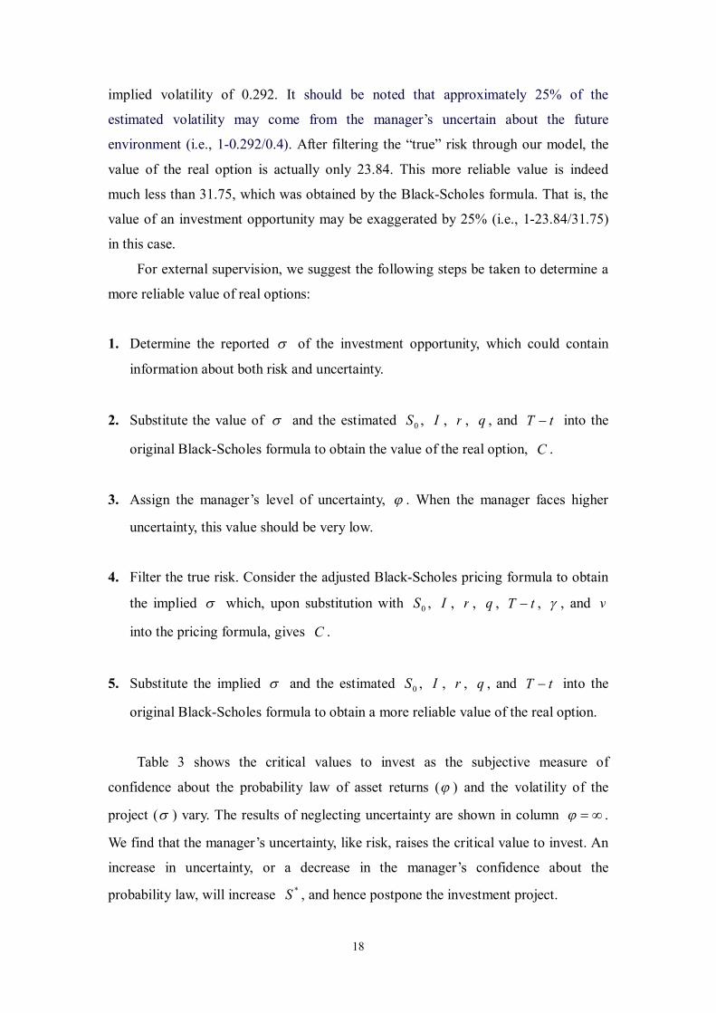
implied volatility of 0.292. It should be noted that approximately 25% of the
estimated volatility may come from the manager’s uncertain about the future
environment (i.e., 1-0.292/0.4). After filtering the “true” risk through our model, the
value of the real option is actually only 23.84. This more reliable value is indeed
much less than 31.75, which was obtained by the Black-Scholes formula. That is, the
value of an investment opportunity may be exaggerated by 25% (i.e., 1-23.84/31.75)
in this case.
For external supervision, we suggest the following steps be taken to determine a
more reliable value of real options:
1. Determine the reported of the investment opportunity, which could contain
information about both risk and uncertainty.
2. Substitute the value of and the estimated 0S , I , r , q , and tT into the
original Black-Scholes formula to obtain the value of the real option, C .
3. Assign the manager’s level of uncertainty, . When the manager faces higher
uncertainty, this value should be very low.
4. Filter the true risk. Consider the adjusted Black-Scholes pricing formula to obtain
the implied which, upon substitution with 0S , I , r , q , tT , , and v
into the pricing formula, gives C .
5. Substitute the implied and the estimated 0S , I , r , q , and tT into the
original Black-Scholes formula to obtain a more reliable value of the real option.
Table 3 shows the critical values to invest as the subjective measure of
confidence about the probability law of asset returns ( ) and the volatility of the
project ( ) vary. The results of neglecting uncertainty are shown in column .
We find that the manager’s uncertainty, like risk, raises the critical value to invest. An
increase in uncertainty, or a decrease in the manager’s confidence about the
probability law, will increase *S , and hence postpone the investment project.

19
4. Conclusions
In this paper, we established a framework that separated risk and uncertainty in
order to evaluate real options. In addition to risk, uncertainty also raised the value of
real options. By using risk and uncertainty interchangeably, we would overestimate
the value of real options. Therefore, we cannot trust the value of real options unless
we clarify and identify risk and uncertainty. The proposed theoretical model
responded well to Alessandri’s (2003) empirical findings. Although the Black-Scholes
pricing formula is user friendly, it nevertheless has drawbacks when applied to the
evaluation of capital projects with higher uncertainty. To our knowledge, any similar
quantitative methods have not hitherto been mentioned in terms of isolating
uncertainty from risk in real options analysis that we consider here.
There are at least two practical benefits of our approach. For internal
management, by parameterizing uncertainty and associated attitudes, our approach
provides a more credible valuation of real options than a rule of thumb. For external
supervisors, our approach helps to detect whether the valuation of real options is
exaggerated.
The separation of ownership and management is a feature of modern corporate
governance. As the owners and managers of the firm belong to different parties, the
conflicts of interest, called agency problems, may arise. Managers could take some
plans to maximize their own profit by sacrificing the owners’ interests. We caution
external supervision, as a solution to mitigate agency problems, about the results from
real options analysis. If risk and uncertainty are unidentifiable, there would be
opportunities for the manager to manipulate the parameter, , in the Black-Scholes
pricing formula to exaggerate the value of an investment opportunity. Moreover, it is
possible that an investment opportunity may be postponed inappropriately.

20
References
Amram, M. and N. Kulatilaka, 1999, Real Options: Managing Strategic Investment in
an Uncertain World, Harvard Business School Press.
Anderson, E., L. Hansen, and T. Sargent, 2000, “Robustness, detection and the price
of risk”, Unpublished Paper, Stanford University.
Boyle, P. and R. Uppal, and T. Wang, 2003, “Ambiguity aversion and the puzzle of
own-company stock in pension plans,” Unpublished Paper, London Business
School.
Bräutigam, J., C. Esche, and A. Mehler-Bicher, 2003, “Uncertainty as a key value
driver of real options,” Conference Paper, 7th Annual Real Options Conference.
Camerer, C. and M. Weber, 1992, “Recent developments in modeling preferences:
uncertainty and ambiguity,” Journal of Risk and Uncertainty, 5, 325-370.
Chen, Z. and L. Epstein, 2002, “Ambiguity, risk and asset returns in continuous time,”
Econometrica, 70, 1403-1443.
Cox, J., S. Ross, and M. Rubinstein, 1979, “Option pricing: A simplified approach,”
Journal of Financial Economics, 7, 229-263.
Davis, G. A., 1998, “Estimating volatility and dividend yield when valuing real
options invest or abandon,” Quarterly Review of Economics and Finance, 38,
725-754.
Dixit, A. and R. Pindyck, 1994, Investment Under Uncertainty, Princeton University
Press.
Dow, J. and S. R. Werlang, 1992, “Uncertainty aversion, risk aversion and the optimal
choice of portfolio,” Econometrica, 60, 197-204.
Duffie, D. and L. Epstein, 1992, “Stochastic Differential Utility,” Econometrica, 60,
353-394.
Ellsberg, D., 1961, “Risk, ambiguity and the Savage axioms,” Quarterly Journal of
Economics, 75, 643-669.
Epstein, L. and S. Zin, 1989, “Substitution, risk aversion and the temporal behavior of
consumption and asset returns: A theoretical framework,” Econometrica, 57,
937-969.
Epstein, L. and T. Wang, 1994, “Intertemporal asset pricing under Knightian
uncertainty,” Econometrica, 62, 283-322.

21
Epstein, L. and J. Miao, 2003, “A two-person dynamic equilibrium under ambiguity,”
Journal of Economic Dynamics and Control, 27, 1253-1288.
Fernandez, P., 2013, “Valuing real options: frequently made errors,” Available at
SSRN: http://ssrn.com/abstract=274855 or http://dx.doi.org/10.2139/ssrn.274855.
Fox, C. and A. Tversky, 1995, “Ambiguity aversion and comparative ignorance,”
Quarterly Journal of Economics, 10, 585-603.
Gilboa, I. and D. Schmeidler, 1989, “Maxmin expected utility with non-unique prior,”
Journal of Mathematical Economics, 18, 141-153.
Hansen, L., T. Sargent, and T. Tallarini, 1999, “Robust permanent income and
pricing,” Review of Economic Studies, 66, 873-907.
Hansen, L. and T. Sargent, 2001, “Acknowledging misspecification in
macroeconomic theory,” Review of Economic Dynamics, 4, 519-535.
Hansen, L. and T. Sargent, 2001, “Robust control and model uncertainty,” American
Economic Review, 91, 60-66.
Hansen, L. and T. Sargent, N. Wang, 2002, “Robust permanent income and pricing
with filtering,” Macroeconomic Dynamics, 6, 40-84.
Hansen, L., T. Sargent, G. Turmuhambetova, and N. Williams, 2002, “Robustness and
uncertainty aversion,” Unpublished Paper, University of Chicago.
Heath, C. and A. Tversky, 1991, “Preferences and beliefs: Ambiguity and competence
in choice under uncertainty,” Journal of Risk and Uncertainty, 4, 5-28.
Ingersoll, J. E., Jr., 2006, “The subjective and objective evaluation of incentive stock
options,” Journal of Business, 79, 453-487.
Knight, F. H., 1921, Risk, Uncertainty and Profit, Houghton Mifflin, Boston.
Kogan, L. and T. Wang, 2002, “A simple theory of asset pricing under model
uncertainty,” Unpublished Paper, Sloan School of Management, MIT.
Lander, D. and G. Pinches, 1998, “Challenges to the practical implementation of
modeling and valuing real options,” Quarterly Review of Economics and Finance,
38, 537-567.
Leslie, K. and M. Michaels, 1997, “The real power of real options,” McKinsey
Quarterly, 3, 4-22.
Lucas, R., 1978, “Asset prices in an exchange economy,” Econometrica, 46,
1429-1445.
Maenhout, P., 2004, “Robust portfolio rules and asset pricing,” Review of Financial
Studies, 17, 951-983.

22
McDonald, R. and D. Siegel, 1986, “The value of waiting to invest,” Quarterly
Journal of Economics, 101, 707-728.
Merton, R., 1971, “Optimum consumption and portfolio rules in a continuous-time
model,” Journal of Economic Theory, 3, 373-413.
Merton, R., 1973, “An intertemporal asset pricing model,” Econometrica, 41,
867-888.
Merton, R., 1980, “On estimating the expected return on the market: An exploratory
investigation,” Journal of Financial Economics, 8, 323-361.
Miao, J. and N. Wang, 2011, “Risk, uncertainty, and option exercise,” Journal of
Economic Dynamics and Control, 35, 442-461.
Nishimura, K. and H. Ozaki, 2007, “Irreversible investment and Knightian
uncertainty,” Journal of Economic Theory, 136, 668-694.
Roubaud, D., A. Lapied, and R. Kast, 2010, “Real Options under Choquet-Brownian
Ambiguity,” Working paper, Université Paul Cézanne.
So, L., 2009, “The role of ambiguity aversion in evaluation of employee stock
options,” Review of Securities & Futures Markets, 21, 87-124.
Trigeorgis, L., 1990, “A real-options application in natural-resource investments,”
Advances in Futures and Options Research, 4, 153-164.
Trigeorgis, L., 1996, Real Options: Managerial Flexibility and Strategy in Resource
Allocation, MIT Press.
Trojanowska, M. and P.M. Kort, 2010, “The Worst Case for Real Options,” Journal of
Optimization Theory and Applications, 146, 709-734.
Uppal, R. and T. Wang, 2003, “Model misspecification and under-diversification,”
Journal of Finance, 58, 2465-2486.

23
Table 1
Parameter Values Used in Calibration
Parameters 0S I v r q tT
Values 100 100 5 0.13 0.04 0.04 10 0.2~0.5 6~
Notes: The parameters are the risk aversion coefficient, rate of return of the investment opportunity, riskless interest rate, dividend yield (shortfall), time to maturity, volatility of the investment opportunity, and subjective measure of confidence about the probability law of asset returns, respectively. We let the values of and vary in the specified ranges to see their influence on the evaluation of real options.

24
Table 2
Subjective Values of Real Options
=6 =8 =10 =12 =14 =16 =18 =20 =100 =
=0.2 25.10 23.02 21.75 20.90 20.29 19.84 19.48 19.20 17.15 16.69 =0.3 32.34 30.46 29.30 28.51 27.94 27.52 27.18 26.91 24.95 24.50 =0.4 39.60 37.73 36.58 35.79 35.23 34.80 34.46 34.19 32.21 31.75 =0.5 46.32 44.43 43.25 42.46 41.88 41.44 41.09 40.82 38.78 38.31
Notes: The table displays the subjective values of real options as the subjective measure of confidence about the probability law of asset returns ( ) and the volatility of the project ( ) vary. Other parameter values are given in Table 1.

25
Table 3
Critical Values of Project Value
=6 =8 =10 =12 =14 =16 =18 =20 =100 =
=0.2 339.28 285.40 261.47 247.99 239.34 233.33 228.91 225.52 204.48 200.44 =0.3 416.94 370.82 347.44 333.32 323.87 317.11 312.02 308.07 282.15 276.88 =0.4 548.78 493.95 465.20 447.50 435.51 426.85 420.30 415.18 381.05 373.98 =0.5 718.51 649.29 612.48 589.64 574.09 562.81 554.27 547.57 502.60 493.21
Notes: The table gives the critical values of the project value as the subjective measure of confidence about the probability law of asset returns ( ) and the volatility of the project ( ) vary. The manager has to defer the investment project until the project value is higher than the critical value. Other parameter values are given in Table 1.