THE REAL OPTIONS EFFECT OF UNCERTAINTY ON

INVESTMENT AND LABOUR DEMAND

Nicholas Bloom

THE INSTITUTE FOR FISCAL STUDIES

WP 00/15

The Real Options Effect of Uncertainty onInvestment and Labor Demand

Nicholas Bloom∗

November 2000

Abstract

This paper shows that, contrary to common beliefs, the real options ef-fect of uncertainty plays no role in the long run rate of investment. This isproven for both the standard investment model with Cobb-Douglas produc-tion and Brownian motion demand, and also for a broader class of modelswith multiple lines of capital, labor and general demand stochastics. Realoptions and irreversibility, however, are shown to play an important role inthe short run dynamics of investment and labor demand. Specifically, theyreduce the short run response of investment and hiring to current demandshocks, and lead to a lagged response to past demand shocks.

Keywords: Investment, labor demand, uncertainty, real options.JEL Classification: D92, E22, D8

Acknowledgments: The author would like to thank Giuseppe Bertola,Steve Bond, Avinash Dixit, Janice Eberly, Tor Klette, Plutarchos Sakellaris,Enrico Saltari, and John Van Reenen for their comments and help. Thisresearch is part of the program of research at the ESRC Centre for theMicro-Economic Analysis of Fiscal Policy at the IFS. Financial support ofthe ESRC is gratefully acknowledged.

Correspondence: nick.bloom@ifs.org.uk; 7 Ridgmount Street, LondonWC1E 7AE, UK.

∗Institute for Fiscal Studies and University College London

1. Introduction

It is commonly understood that the real options effect of uncertainty reduces

investment1. To be precise, when investment is irreversible so that capital cannot

be resold for its full purchase price, a firm’s optimal investment rule takes on a

threshold form. Investment will only occur when demand rises to some upper

threshold while disinvestment will occur only when demand falls to some lower

threshold. It has often been assumed that because uncertainty raises the upper

threshold for investment2, it reduces the long run rate of investment.

This appears to be confirmed by a variety of papers which find an inverse

relationship between uncertainty and investment. Caballero (1991) and Lee and

Shin (2000) demonstrate that in a two period model in which firms start off

with no capital stock the real options effect of uncertainty unambiguously acts to

reduce investment in the first period. Pindyck (1993) and Sakellaris (1994) report

that in a competitive multi-period (three or more periods) model of investment in

which firms again start off with no initial capital stock the real options effect of

uncertainty also unambiguously reduces first period investment. And Dixit and

Pindyck’s (1994) survey on the investment under uncertainty literature implies a

negative impact of real options on investment when they report that

”a larger σ [the standard deviation of demand] means a lower long-run

average growth rate of the capital stock, and thus less investment on

average” [page 373]

1The real options effect of uncertainty is defined as ”the effect of uncertainty that arises froma firm’s option to choose the timing of its investment” when this investment is irreversible.

2The effect of uncertainty in raising the investment threshold is demonstrated, for example,by Bertola (1988), Pindyck (1988), Dixit (1989), Bentolila and Bertola (1990), Bertola andCaballero (1994), Dixit and Pindyck (1994) and Abel and Eberly (1996).

2

In this paper we argue that these existing papers cannot be used to draw

inferences about the real options effect of uncertainty on long run investment

since they either amalgamate differing short and long run impacts, or introduce

Jensen’s inequality effects in to demand growth. This paper distinguishes the real

options effect in the short run from its effect in the long run, and controls for

these Jensen’s inequality effects. In section 2 we show that real options play no

role in determining the long run rate of investment.

The intuition for this result is that while the real option effect of uncertainty

increases the investment threshold, reducing the rate of investment in times of

strong demand, it also lowers the disinvestment threshold, reducing the rate of

disinvestment in times of weak demand. These effects on the rate of investment

and the rate of disinvestment exactly cancel out in the long run. This result is

proven for both the standard Cobb-Douglas production function and Brownian

motion demand model (proposition 1) and also a more general class of multi-

capital production functions and stochastic demand processes (proposition 2). As

a corollary to proposition 1 we also show that the negative effect of uncertainty

on long run investment quoted above from Dixit and Pindyck (1994) derives from

a Jensen’s inequality effect and is unrelated to real options.

Although real options do not affect long run investment, it is shown in section

3 that they play an important role in the short run dynamics of investment and

labor demand. The separation of the investment/disinvestment thresholds and the

hiring/firing thresholds is proven to reduce the short run responsiveness to demand

shocks at any level of aggregation (proposition 3). This explains the findings of

Caballero (1991), Pindyck (1993), Sakellaris (1994) and Lee and Shin (2000) whose

3

assumption that firms start off with no capital is critical since it ensures that first

period investment will necessarily be positive. Because higher uncertainty reduces

the investment response it reduces this first period investment in their model and

generates a negative real options effect of uncertainty on investment. We show

that the investment and hiring response to demand shocks is convex with larger

shocks leading to proportionally larger responses (proposition 4). In addition to

reducing the short run responsiveness, real options and irreversibilities are also

shown to induce strong dynamics into the investment and hiring process, leading

to lagged responses to past demand shocks (proposition 5).

These predictions from real options and irreversibility - in particular the low

short run responsiveness and the longer lagged response - match the stylized facts

from estimating firm, industry and macro level investment and labor demand

models3. Estimates of the short run elasticities of investment and hiring to de-

mand shocks are generally moderate in size, with point estimates on annual data

often around one quarter and one half respectively. Additional lagged responses,

however, lead to a much higher long run response, with some suggestion that the

long run elasticities of both factors is about unity.

Related literature to this paper includes Abel and Eberly (1995) who exam-

ine the influence of uncertainty on the level of the capital stock under complete

irreversibility with no depreciation for a range of parameter values, and find an

ambiguous response. Our work complements these results by examining the real

options effect of uncertainty and irreversibility on long run investment - that is on

the growth of the capital stock. Since we find no impact on the long run growth of

the capital stock this suggests that any real options effects of uncertainty on the

3See for example Chirinko (1993) on investment and Hamermesh (1993) on labor demand.

4

level of the capital stock are stationary and independent of long run investment.

Our results are also fully analytical, unambiguous, and obtained for a more gen-

eral model which allows for partial irreversibility, depreciation, multiple-lines of

capital, and broader demand stochastics.

The impact of real options and irreversibilities on short run dynamics has

previously been noted by Bertola and Caballero (1994), who model aggregate

investment in an economy composed of a continuum of homogenous firms, each

operating with a single line of irreversible capital. We extend these results in

a number of directions by generalizing to firms with multiple-lines of partially

irreversible labor and capital, allowing for a less restrictive demand processes, al-

lowing for heterogeneity across firms, and dispensing with the need for aggregation

across a large numbers of units. This allows us to make predictions on the short

run dynamic effects of real options on investment and hiring in data-sets at all

levels of aggregation, from the plant and firm level up to the industry and macro

level, with these being robust to a variety of production and demand processes.

Finally, a number of papers cited above4 also examine a result, demonstrated

in Hartman (1972) and Abel (1983), that if a firm can freely adjust its labor force

used in production after investment has been undertaken, this can lead the mar-

ginal revenue product of capital to be convex in price, so that greater uncertainty

may increase the level of the capital stock. The result, however, depends on par-

ticular modelling assumptions over both the revenue function and the form of the

demand shock so that, for example, if the demand shock is modelled as a quantity

rather than a price shock this uncertainty effect disappears or can even be re-

versed. This Hartman-Abel effect of uncertainty also requires firms to undertake

4Caballero (1991), Pindyck (1993), Sakellaris (1994) and Lee and Shin (2000).

5

frequent adjustment of its labor force, which if labor is believed to be subject to

adjustment costs, may not be optimal. Since our results are valid both with and

without this uncertainty effect we do not discuss this issue any further.

The plan of the paper is as follows. Section 2 starts by examining the standard

model with a single line of capital and flexible labor and demonstrates that real

options have no impact on the long run rate of investment. We then consider a

broad class of models which allow for multiple lines of capital and inflexible labor

under any degree of aggregation, and show that real options still play no role

in determining the long run rate of investment. Section 3 then uses this general

framework to consider the short run effects of real options and irreversibilities, and

proves that these will retard the investment and hiring response to demand shocks,

and lead to a dynamic lagged response to demand shocks. Some concluding

remarks are then made in section 4.

6

2. Long Run Impact of Real Options on Investment

We start off by examining a stylized investment model with one line of capital and

flexible labor which is commonly used in the irreversible investment literature5.

2.1. The Standard Model with a Single Line of Capital and FlexibleLabor

The firm’s revenue function, R(K,P ), in terms of its capital stock (K) and its

demand conditions (P ) is modelled as having the following form

R(K,P ) =1

aP 1−aKa (2.1)

where this can be shown to nest a Cobb-Douglas production function and an iso-

elastic demand curve. In this setup labor is assumed to be a completely flexible

factor of production and has been optimized out of the revenue function. We

assume that the firm’s demand conditions follow a Brownian motion process with

drift µ and variance σ2. The firm is assumed to maximize the expected present

value of sales revenues, minus the cost of buying capital at a price B, plus the

proceeds received from selling capital at a price S, where B > S. The optimal

investment strategy then maximizes its total discounted profits

max{I(s)}

Et

½Z ∞

t

exp−r(s−t)(1

aP 1−a(s)K(s)ads−BdI+(s) + SdI−(s))

¾(2.2)

subject to dK(t) = −δKdt+ I(t)

where r is the discount rate I+ denotes positive investment and I− denotes neg-

ative investment, and δ is the rate of capital depreciation.

5This model of partial irreversibility is taken directly from Abel and Eberly (1996) and isa generalisation of the complete irreversibility case in Bertola (1988) and Dixit and Pindyck(1994) Chapter 11.

7

Abel and Eberly (1996) demonstrate that the profit maximizing investment

behavior can be described in terms of the firm’s current marginal revenue product

of capital P 1−aKa−1, and an investment and disinvestment threshold, which is

summarized in Table 1 below. These thresholds are represented by the investment

and disinvestment user costs of capital, CI and CD respectively6, and two real

options terms ΦI > 1 and ΦD > 1.

Table 1: The threshold behavior of investment with real options

Invest if: P 1−aKa−1 = CIΦI

Do Nothing if: CD/ΦD < P1−aKa−1 < CIΦI

Dis—Invest if: P 1−aKa−1 = CD/ΦD

After taking logs, these thresholds provide bounds for the logged capital stock

under partial irreversibility, which using lower case to denote logged variables,

can be stated as follows

p−µcI + φI1− a

¶≤ k ≤ p−

µcD − φD1− a

¶(2.3)

To pinpoint the impact of real options we make a ceteris paribus comparison to

the situation in which the firm acts as if it has no option to delay its investment.

By modelling the firm as if it has a now or never investment choice we can turn off

the real options effect but keep all other parameters and the evolution of demand

constant7. Under this hypothetical alternative we know from Jorgenson (1963)6Jorgenson (1963) demonstrates that when capital costs a constant price B to buy, the

investment user cost of capital can be expressed as CI = (r + δ)B. This can be generalisedfor capital resale at a constant price S, to denote the disinvestment user cost of capital asCD = (r + δ)S.

7This ‘no real options’ scenario can be equivalently described as the situation in which thefirm always acts as if the current level of demand will extend into the future with completecertainty.

8

that the firm will only invest when its marginal revenue product of capital is equal

to its investment user cost of capital CI , and only disinvest when its marginal

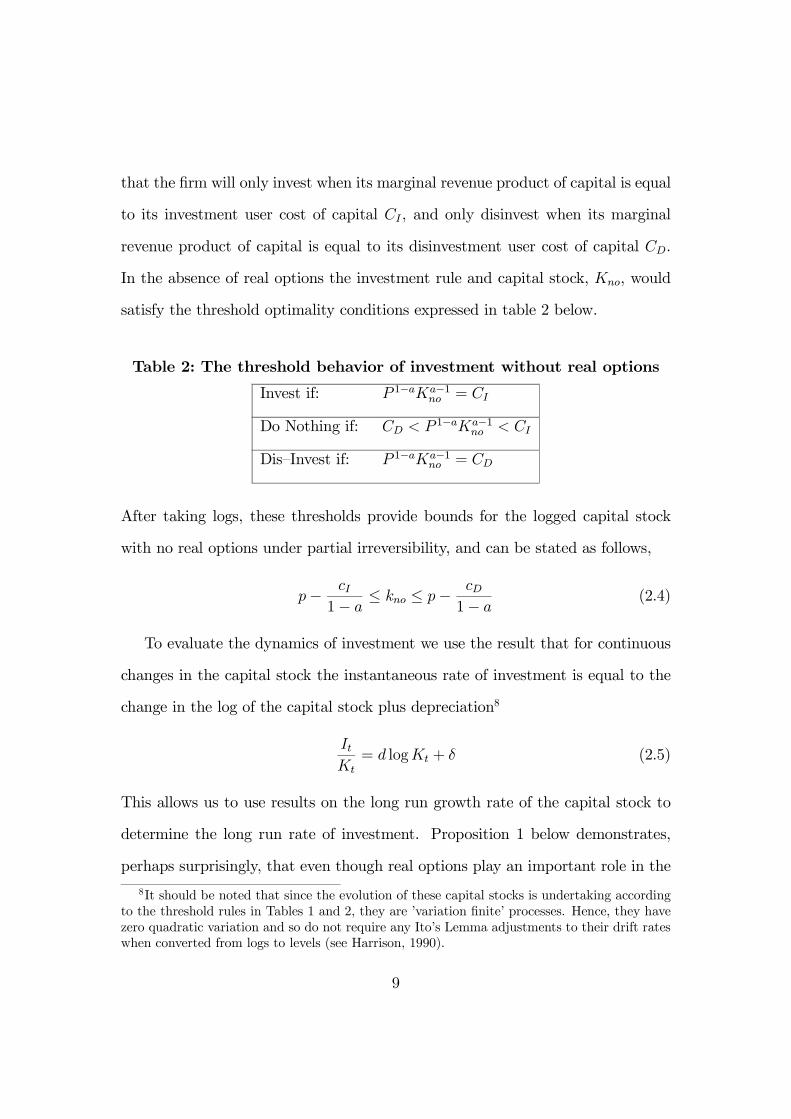
revenue product of capital is equal to its disinvestment user cost of capital CD.

In the absence of real options the investment rule and capital stock, Kno, would

satisfy the threshold optimality conditions expressed in table 2 below.

Table 2: The threshold behavior of investment without real options

Invest if: P 1−aKa−1no = CI

Do Nothing if: CD < P1−aKa−1

no < CI

Dis—Invest if: P 1−aKa−1no = CD

After taking logs, these thresholds provide bounds for the logged capital stock

with no real options under partial irreversibility, and can be stated as follows,

p− cI1− a ≤ kno ≤ p−

cD1− a (2.4)

To evaluate the dynamics of investment we use the result that for continuous

changes in the capital stock the instantaneous rate of investment is equal to the

change in the log of the capital stock plus depreciation8

ItKt= d logKt + δ (2.5)

This allows us to use results on the long run growth rate of the capital stock to

determine the long run rate of investment. Proposition 1 below demonstrates,

perhaps surprisingly, that even though real options play an important role in the

8It should be noted that since the evolution of these capital stocks is undertaking accordingto the threshold rules in Tables 1 and 2, they are ’variation finite’ processes. Hence, they havezero quadratic variation and so do not require any Ito’s Lemma adjustments to their drift rateswhen converted from logs to levels (see Harrison, 1990).

9

determination of the investment thresholds, they play no limiting role in long run

investment.

Proposition 1: Real Options have no limiting effect on long run investment.

Proof: For partially irreversible investment combining the conditions (2.3) and

(2.4) we find that the difference between the capital stock with real options and

without real options is bounded by a finite constant,

− log φI1− a ≤ k − kno ≤ log φD

1− a (2.6)

Hence, K and Kno have the same long run limiting9 growth rate since

limT→∞

1

T| log(KT+t/Kt)− log(Kno,T+t/Kno,t)| = lim

T→∞1

T|(log(KT+t/Kno,T+t)− log(Kt/Kno,t)|

≤ limT→∞

1

T| log φI1− a +

log φD1− a | (2.7)

= 0

By (2.5) they also have the same long run rate of investment. For completely

irreversible investment the distance between the capital stock with real options

and without real options is, after any initial common investment episode, a fixed

distance apart10,

k − kno = − logφI1− a (2.8)

Hence, by the same logic as above they also have the same long run rate of

investment.9This and all other limits in the paper are the standard deterministic limits.10For complete irreversibility the (positive investment) rules from Tables 1 and 2 are still

optimal, so that during any common investment episode the levels of the capital stock withoptions and without options will be logφU1−a apart. Since subsequent depreciation imparts a linear

trend to both capital stocks this log φU1−a gap between the two levels will persist from then onwards.

10

These results are independent of any assumptions on the rate of capital de-

preciation, the rate of demand growth, the degree of uncertainty or the degree of

irreversibility.

!

The intuition for this proof is that the capital stocks with and without real

options are both contained within the real options investment thresholds. These

thresholds are a fixed and bounded distance apart so that the gap between the two

capital stocks is also fixed and bounded. Over time the importance of this fixed

gap for long run investment tends to zero, as the evolution of demand becomes

the first order determinant of investment. This is illustrated in figure 1, which

plots in bold the investment profile for the capital stock with real options and

without real options for a random 10 year realization of logged demand11. Also

plotted in figure 1 in feint are the investment and disinvestment thresholds for

the capital stock with real options.

FIGURE 1 ABOUT HERE

In figure 1 both the capital stocks with and without real options have been

normalized to start off at one unit so that total cumulative investment can be

measured from the current level of the capital stock. It can be seen that these

two capital stocks evolve in a similar manner to each other. Figure 2 plots the

evolution of these two capital stocks for the same demand process continued over a

11Logged demand is drawn from a Brownian process with 5% drift and 20% standard deviation.Returns to capital are assumed homogenous of degree 0.75, consistent with constant returns toscale production and a price elasticity of 4. Capital depreciates at 10% per year, costs $1 perunit to buy and can be resold for $0.75 per unit. The firm’s annual discount rate is 10%.

11

fifty year period from which the equivalence between the long run rates of growth

is much clearer12.

FIGURE 2 ABOUT HERE

While the real options effect of uncertainty plays no role in long run investment,

there is a specific case in which uncertainty does play a long run role by directly

affecting the growth rate of logged demand. This effect is independent from real

options.

Corollary to Proposition 1: Uncertainty can decrease (increase) expected

long run investment, independently of real options and irreversibility, if logged

demand is concave (convex) in the Brownian motion term.

Proof: From the definition of the thresholds for the level of capital stock with

and without real options, equations (2.3) and equations (2.4), we can see that the

long run growth rate of both levels of capital will be equal to the long run growth

rate of logged demand,

limT→∞

1

T| log(KT+t/Kt)| = lim

T→∞1

T| log(Kno,T+t/Kno,t)|

= limT→∞

1

T|(log(PT+t/Pt)|

Jensen’s inequality states that long run growth of demand will be decreasing (in-

creasing) in the variance of demand if logP is concave (convex) in the underlying

12For Ss models with fixed costs of adjustment, for example as analyzed by Grossman andLaroque (1990), the long run rate of investment is also independent from any option value effectsof uncertainty, since the investment rule takes on a similar threshold form.

12

Brownian motion process. But, since this affects the level of the capital stock both

with and without real options, this Jensen’s effect of uncertainty is independent

of real options.

!

This explains Dixit and Pindyck’s (1994) result that the expected long run

rate of investment is equal to µ− σ2

2, and so reduced by higher uncertainty, since

logged demand is concave in the level of demand. But this Jensen’s effect is not

a robust theoretical prediction since it relies on the initial assumptions on the

functional form of the demand process. For example, if we assume that logged

demand, rather than the level of demand, is a Brownian motion process with

mean µ and standard deviation σ, then this effect of uncertainty would disappear

entirely.

2.2. A Model With Multiple Lines of Capital and Labor AdjustmentCosts

The investment model outlined above, as is common in the literature, treats all

types of capital within the firm as homogenous and labor as completely flexible

because this makes the firm’s optimization problem analytically tractable. But

even a cursory glance at establishment and firm level data will reveal that it is

common for firms to operate at several different production locations, across in-

dustry classifications, and with different capital mixes and vintages. Furthermore,

since at least the work of Oi (1962) it has been recognized that hiring and firing

workers involves recruitment, training, reorganization and compensation costs,

which makes labor a costly factor to adjust. We generalize the firm level produc-

tion function to allow for N separate lines of capital and M types of labor and a

13

more flexible demand process. This is done in a general way by considering the

class of models which satisfy the following three assumptions13:

1. The sales function is jointly concave and homogenous of degree λ in all N

lines of capital andM types of labor, where λ < 1. Individual lines of capital

and types of labor within each plant are also complementary in production14.

2. Lines of capital cost B = {B1, B2, ...BN} to buy and can be resold forS = {S1, S2, ...SN} where 0 < S < B. Labor can be hired at a cost H =

{H1,H2, ...HM} and fired at a cost F = {F1, F2, ...FM}, where these costsinclude the present discounted value of all future wage payments, and 0 <

F < H.

3. The firm level demand shock has a multiplicative impact upon revenue and

is generated by a stationary Markov process15.

Since firms may operate using several lines of capital and types of labor we

have to generalize our threshold investment rule. Eberly and Van Mieghem (1997)

demonstrate that the investment policy of a production plant with N lines of

capital and M types of labor satisfying conditions (1) to (3) will be of a multi

dimensional threshold form as characterized in Table 3.

13This class of models includes the Cobb-Douglas production and Brownian demand modelwe discussed previously in section (2.1).14This complementarity is defined such that for a production function

F (K1,K2...KN ;L1, L2...LM) the marginal product of any individual factor of productionis increasing in every other factor of production. For example, ∂F (K1,K2...KN)/∂Ki wouldbe increasing in all Kj , j 6= i. This condition is technically known as supermodularity and isdescribed in more detail in Dixit (1997).15Stationarity implies that this process does not depend on time, while the Markov property

implies that the future behaviour of the process depends on its present position but not on howit got there.

14

Table 3: N+M dimensional investment and hiring threshold behavior

For Lines of Capital i = 1, 2, ...N For Types of Labor j = 1, 2, ...MInvest if: Ki = K

Ii Hire if: Lj = L

Hj

Do Nothing if: KIi < Ki < K

Di Do Nothing if: LHj < Lj < L

Fj

Dis—Invest if: Ki = KDi Fire if: Lj = L

Fj

For this more general set up we demonstrate in proposition 2 below that once

again real options play no role in determining long run investment.

Proposition 2: For models satisfying assumptions (1) to (3) real options have

no effect on the long run rate of investment.

Proof: In Appendix A

!

This suggests that even in quite general models of production and investment,

after conditioning on demand growth to remove any Jensen’s inequality effects,

uncertainty plays no role in determining the long run rate of investment.

3. The Short Run Impact of Real Options and Irreversibil-ity on Investment and Labor Demand

The combination of real options and irreversibility do play an important role,

however, in shaping the short run response to demand shocks. To explore this

issue we first develop a methodology for characterizing these responses which is

robust to any degree of aggregation. This is important because it enables us to

make predictions on the dynamics of investment and hiring at the establishment,

firm, industry, and macro level - thereby developing results that apply to data at

the much lower levels of aggregation that is commonly used in empirical work. To

ensure as wide a generality as possible we also maintain the multiple line of capital

15

and inflexible labor model outlined by assumptions (1) to (3) in section (2.2).

While our results will be stated for investment and hiring, to avoid repetition

we will prove them only for investment, with the proof for hiring following by

symmetry16.

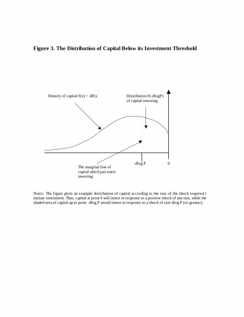
First, we define F (−x) to be the cumulative distribution of log capital withineach firm according to the size of the demand shock x required to move the cap-

ital up to its investment threshold. This implies, for example, that F (0) = 1

because all lines of capital will be either on or below their investment demand

threshold and so require a shock of zero or greater to start investing. In contrast,

if F (−∆ logP ) = 0, this would imply that all lines of capital would start investingafter a (presumably large) demand shock of size ∆ logP . Figure 3 plots an ex-

ample density function, f(x) = dF (x), of capital below its investment threshold

with the shaded area representing F (−d logP ), the lines of capital which wouldinvest after a demand shock of size d logP .

FIGURE 3 ABOUT HERE

Second, we define the investment function for capital at each point x of this

cumulative distribution F (−x) as follows17

d logK(−x) = I(−x,∆ logP ) where I(−x,∆ logP ) ≥ 0 if ∆ logP ≥ x

and I(−x,∆ logP ) = 0 if ∆ logP ≤ x16Note that we define the rate of labor hiring as the change in the logged labor force.17This investment function actually also depends on the whole distribution of capital be-

low the threholds F (.), so could be fully written out for a position x and shock ∆ logP asI(−x,∆ logP,F (.)). However, since this does not effect the discussion of the main results thisis compressed to the shorter form I(−x,∆ logP ) in the main text.

16

The right hand side conditions follow by the definition of −x as the smallestdemand shock required to move capital at that position up to the investment

threshold. This investment function will be increasing in the size of the demand

shock so that ∂I(−x,∆ logP )∂∆ logP

≥ 0. For firms with multiple lines of capital this

investment function will also be convex (increasing at an increasing rate) due to

the assumed complementarity of capital in production, so that ∂2I(−x,∆ logP )(∂∆ logP )2

≥ 0.Combining these two definitions we can characterize total firm level investment

to a demand shock of size ∆ logP as

∆ log(K) =

Z 0

−∆ logPI(x,∆ logP )dF (x) (3.1)

One important effect of real options and irreversibility is to reduce the invest-

ment and hiring response to a demand shock. This arises because firms will act

more cautiously when capital and labor is partially irreversible and their market

conditions are uncertain - any investment and hiring represents a gamble from

which the firm can not easily extricate itself if conditions turn bad. This is noted

in proposition 3 below

Proposition 3: Real options and irreversibility will reduce the responsiveness

of investment and hiring to demand shocks.

Proof : In response to a positive demand shock of size ∆ logP the investment

response across all lines of capital will be

∆ log(K) =

Z 0

−∆ logPI(x,∆ logP )dF (x) (3.2)

≤Z 0

−∆ logP

1

1− λ(∆ logP + x)dF (x)

=1

1− λµ∆ logP −

Z 0

−∆ logPF (x)dx

¶17

≤ 1

1− λ∆ logP

where the second line follows because I(x,∆ logP ) ≤ 11−λ(∆ logP + x) by the

complementarity of capital in production (see appendix B for details), and the

third line follows by integration by parts. If there is any capital lying below the

investment threshold, so that F (−x) > 0 for some x > 0, we obtain the strict

inequality that ∆ log(K) < 11−λ∆ logP . To isolate the impact of real options and

irreversibility we make the comparison to the hypothetical completely reversible

level of capital, KR. For this reversible capital we show in appendix B that

∆ log(KR) =1

1− λ∆ logP (3.3)

Combining (3.2) and (3.3) demonstrates that the investment response is lower

under partial irreversibility than under complete reversibility.

!

The intuition for this result is that the region of inaction between the invest-

ment/disinvestment thresholds and the hiring/firing thresholds acts as a buffer

against demand shocks. Within this region the response to shocks will be zero

unless they are large enough to ensure that capital and labor are moved up against

their investment and hiring thresholds. And even when the demand shock is large

enough to ensure this happens the investment and hiring response will still be

reduced by the zone of inaction.

FIGURE 4 ABOUT HERE

Figure 4 plots an investment response, as an example, for a an economy com-

prised of a set of firms operating with a single line of capital and flexible labor,

18

and where these firms are uniformly distributed between their investment and

disinvestment thresholds. We can see that the investment response to a demand

shock under partial irreversibility (the curved darker line) is always smaller than

the investment response under complete reversibility (the straight lighter line).

It can also be seen that while the demand response is always lower under par-

tial irreversibility, this response is proportionally larger for larger shocks than for

smaller shocks. This leads to a low but increasing and convex investment and

hiring response to demand shocks, as noted in proposition 4 below.

Proposition 4: Real options and irreversibility will lead to an increasing

convex investment and hiring response to demand shocks.

Proof: Taking the first derivative of the investment response in (3.1) with

respect to the demand shock yields a positive result, simply indicating that larger

shocks lead to more investment

∂∆ log(K)

∂∆ logP=

Z 0

−∆ logP

∂I(x,∆ logP )

∂∆ logPdF (x) ≥ 0 (3.4)

Taking the second derivative we see that the investment response is also increasing

in the size of the shock

∂2∆ log(K)

∂(∆ logP )2=

Z 0

−∆ logP

∂2I(x,∆ logP )

(∂∆ logP )2dF (x) +

∂I(−x,∆ logP )∂∆ logP

|x=−∆ logPdF (−∆ logP )

≥ 0

where the first term is non-negative by the assumed complementarity of different

lines of capital in production and the second term is non-negative by the non-

decreasing nature of cumulative distribution functions.

!

19

This prediction matches the results of Caballero, Engel and Haltiwanger (1997)

and Cooper and Haltiwanger (2000), who estimate employment and investment

functions respectively on a panel of US establishment level data, and find a convex

and increasing response.

Finally, in addition to the reduction in the short run response of investment

and hiring to demand shocks, real options and irreversibility also lead this re-

sponse to be spread out over time, imparting rich and persistent dynamics to

these processes. This is noted in proposition 5 below.

Proposition 5: Real Options and irreversibility will lead investment and

hiring to be increasing in all past demand shocks.

Proof: In Appendix C

!

This can be interpreted in terms of the basic concept of pent up demand.

Firms and industries with a history of strong recent demand growth will have a

distribution of capital and labor lying close to their investment threshold and will

display a strong investment and hiring response, while firms with a recent history

of bad demand shocks will be less disposed to hire or invest. Empirically this

will lead investment and labor demand to appear to respond to both current and

lagged demand shocks. This matches the stylized facts from estimating firm and

macro investment and labor demand equations. These display lagged responses

to demand shocks usually spread over several quarters and years18.

18See, for example, Chirinko (1993) and Hammermesh (1993).

20

4. Conclusion

In this paper we have shown that real options play no role in determining the long

run rate of investment. This is demonstrated for both the standard model with

Cobb-Douglas production and Brownian demand shocks, and also for a broader

class of models with multiple lines of capital, inflexible labor and a generalized

demand process. However, real options and irreversibilities are shown to play an

important role in shaping the short run dynamics of investment and hiring. They

reduce the short run response of investment and hiring to current demand shocks

and create lags in the response to past demand shocks.

The predictions of this model are consistent with the stylized facts from esti-

mating firm, industry and macro level investment and labor demand equations.

Hence, using real options to build a structural framework for estimating invest-

ment and labour demand should help to bridge the gap between what is often em-

pirically preferable (reduced form models) and what is often theoretically prefer-

able (their structural counterparts). And from the policy perspective, the time

varying response elasticity of investment and employment over the business cycle

can be explained by variations in the degree of macro uncertainty. Thus using

measures of the current degree of macro uncertainty could improve the predictions

of the response elasticities of investment and employment, helping policymakers

to better model the effects of tax and interest rate changes.

21

Appendix APROOF OF PROPOSITION 2:

For a plant with N+M lines of capital and types of labor satisfying assump-

tions (1) to (3) we define V (K,L, P ) to be its value function given its current

capital stock K = {K1, K2, ...KN}, labor force L = {L1, L2, ...LM}, and demandcondition P . By theorems 9.6, exercise 9.9 and theorem 9.10 respectively of

Stokey et al. (1983) this value function will inherit the concavity and homogene-

ity properties of plant level sales and will be once continuously differentiable. We

define U = {B1, ...BN , H1...HM} and D = {S1, ...SN , F1...FM} to be the combinedN+M dimensional {buy,hire} and {sell,fire} prices of capital and labor. Following

Eberly and Van Mieghem (1997) we can define the plants investment and hiring

thresholds by the vector of first differential of V (K,L,P ) with respect to each line

of capital and type of labor,

D ≤ ∇V (K,L,P ) ≤ U (4.1)

Since this value function is homogenous of degree one19 in (K,L, P1

1−λ ) its vector

of first derivatives will be homogeneous of degree zero in (K,L, P1

1−λ ) so that this

condition can be re-written as

D ≤ ∇V (KP− 11−λ ,LP−

11−λ , 1) ≤ U (4.2)

By the concavity of ∇V (K,L,P ) this defines a bounded continuation region suchthat

P1

1−λΓIK ≤ K ≤ P

11−λΓDK (4.3)

19By assumptions (1) to (3) sales is homogeneous of degree λ inK and L, and homogeneous ofdegree one in P (due to the multiplicative nature of the shock), and so sales is jointly homogenousof degree one in (K,L,P

11−λ ).

22

P1

1−λΓHL ≤ L ≤ P

11−λΓFL (4.4)

where ΓIK , ΓDK ∈ RN and ΓHL , Γ

FL ∈ RM , with these being functions of the

curvature of the value function and the cost of reversibility. Hence for capital we

can write1

1− λ logP + logΓIK ≤ logK ≤ 1

1− λ logP + logΓDK (4.5)

By revealed preference these optimal investment and disinvestment thresholds

contain the investment and disinvestment thresholds for a firm that ignores its

option to delay the investment decisions so that

logΓIK − logΓDL ≤ logK− logKno ≤ logΓDK − logΓIK (4.6)

where logKno is the vector of no real options capital stocks.

Following the same logic as in proposition 1 we can show that logK and

logKno have the same long run limiting growth rate since

limT→∞

1

T| log(KT+t/Kt)− log(Kno,T+t/Kno,t)| = lim

T→∞1

T|(log(KT+t/Kno,T+t)− log(Kt/Kno,t)|

≤ limT→∞

1

T| logΓI + logΓD| (4.7)

= 0

!

Appendix BNOTES FOR THE PROOF OF PROPOSITION 3:

From equation (4.1) above it can be seen that for completely reversible capital

and labor we have

∇KV (KP−11−λ, 1) = r (4.8)

23

where r is the reversible cost of capital. Thus logK = 11−λ logP + logΓ

rK. The

investment response to a demand shock can then be written as, ∆ logKi =

11−λ∆ logP , which, since this holds for the log of each line of capital, holds for the

log of the total capital stock,

∆NXi=1

logKi =

PNi=1 dKiPNi=1Ki

(4.9)

=1

1− λ∆ logP. (4.10)

To show that

I(x,∆ logP ) ≤ 1

1− λ(∆ logP + x). (4.11)

it is sufficient to note that under irreversibility every line of capital and type of

labor may not be adjusting, and because these are supermodular (complementary)

in production, the investment response to a demand shock at the investment

threshold will be less than the reversibility case where all factors of production

would adjust. This inequality will be strict if production is strictly supermodular

and some factors do not adjust fully.

!

Appendix CPROOF OF PROPOSITION 5:

The approach of this proof is to demonstrate that for any demand shock in

period t a lagged positive demand shock in any period t− s, s > 0, will increaseinvestment in period t. And the larger the demand shock in period t − s thelarger the increase in investment in period t. Thus current investment will be an

increasing function of past demand shocks.

24

Suppose in the absence of a some past demand shock the cumulative density

of capital below the investment thresholds has the form F (x). The investment

function at each point x in response to a demand shock ∆ logPt takes the value

I(−x,∆ logPt, F (.)), where we use the fuller notation which accounts for the im-pact of the distribution of capital on the investment response of each line of capital.

Since all lines of capital are (weakly) complimentary in production the investment

function will be weakly increasing in all weakly decreasing transformations of F (.)

across its support.

Now consider a counter factual in which the firm experienced a shock in pe-

riod t − s of magnitude ∆ logPt−s > 0 so that the distribution below the in-

vestment threshold is now characterised by gF (.). We can then define the newinvestment function at each point x on the old cumulative density function by

I(−x,∆ logPt,gF (.)). For each point x on the old cumulative density functionthis new investment function must be greater or equal to than the old investment

function since gF (.) ≤ F (.) across the support of x, because the lagged demand

shock will have moved all lines of capital closer to their investment thresholds.

Hence, using our characterization for investment we can write

^∆(logK) =

Z 0

−∆ logPt−g(F (.),gF (.)) I(−x,∆ logPt,gF (.))dF (x)

≥Z 0

−∆ logPtI(−x,∆ logPt,gF (.))dF (x)

≥Z 0

−∆ logPtI(−x,∆ logPt, F (.))dF (x)

= ∆ log(K)

where g(F (.),gF (.)) ≥ 0 is a positive function reflecting the impact of past demandshocks on the density of capital which will invest today. Hence, current investment

25

is increasing in lagged demand shocks. Since ,I(−x,∆ logPt,gF (.)) is increasing innegative transformations of gF (.), and gF (.) is decreasing in the size of the laggeddemand shock, current investment will display a larger response to larger lagged

demand shocks. Since this result holds by symmetry for negative demand shocks

the proof is complete.

!

26

ReferencesAbel, Andrew. (1983) ”Optimal Investment under Uncertainty”, American

Economic Review, March vol.73, pp.228-33.

Abel, Andrew. and Eberly, Janice. (1995) ” The Effects of Irreversibility and

Uncertainty on Capital Accumulation”, NBER Working Paper no. 5363.

Abel, Andrew. and Eberly, Janice. (1996) ”Optimal Investment with Costly

Reversibility”, Review of Economic Studies,. vol. 63, pp. 581-593

Bentolila, Samuel. and Bertola, Giuseppe. (1990), ”Firing Costs and Labor

Demand: How Bad is Eurosclerosis?”, Review of Economic Studies, vol 57, pp.

381-402.

Bertola, Giuseppe. (1988), ”Irreversible Investment”, Massachusetts Institute

of Technology doctoral thesis, re-printed in Research in Economics (1998), vol.

52, pp. 3-37.

Bertola, Giuseppe. and Caballero, Ricardo. (1994) ”Irreversibility and Aggre-

gate Investment” Review of Economic Studies 61: 223-246.

Caballero, Ricardo (1991) ”On the Sign of the Investment-Uncertainty Rela-

tionship”, American Economic Review (March): 279-288.

Caballero, Ricardo., Engel, Eduardo. and Haltiwanger, John. (1997), ”Aggre-

gate Employment Dynamics: Building from Microeconomic Evidence”, American

Economic Review (March): pp. 115-137.

Chirinko, Robert. (1993), ”Business Fixed Investment Spending: Modeling

Strategies, Empirical Results, and Policy Implications”, Journal of Economic

Literature vol. XXXI, pp.1875-1911.

Cooper, Russell., Haltiwanger, John. and Power, Laura. (1999) ”Machine

27

Replacement and the Business Cycle: Lumps and Bumps”, American Economic

Review.

Cooper, Russell. and Haltiwanger, John. (2000) ”On the Nature of Capital

Adjustment Costs”, NBER working paper no W7925.

Dixit, Avinash. (1989). ”Entry and Exit Decisions under Uncertainty”. Jour-

nal of Political Economy 97 (June): 620-638.

Dixit, Avinash. and Pindyck, Robert. (1994) ”Investment Under Uncertain-

ty”, Princeton University Press, Princeton, New Jersey.

Dixit, Avinash. (1997). ”Investment and Employment Dynamics in the Short

Run and the Long Run”, Oxford Economic Papers, vol. 49 pp.1-20.

Eberly, Janice. and Van Mieghem, Jan. (1997), ”Multi-Factor Dynamic In-

vestment under Uncertainty”, Journal of Economic Theory, vol. 75, pp. 345-387.

Grossman, Sanford. and Laroque, Guy. (1990), ”Asset Pricing and Opti-

mal Portfolio Choice in the Presence of Illiquid Durable Consumption Goods”,

Econometrica vol. 58, pp.25-51

Harrison, Michael. (1985) Brownian Motion and Stochastic Flow Systems,

Krieger Publishing Company.

Hartman, Richard. (1972) ”The Effects of Price and Cost Uncertainty on

Investment”, Journal of Economic Theory, October 1972, 5, pp. 258-66.

Hamermesh, Daniel. ”Labor Demand” Princeton University Press, Princeton,

New Jersey.

Jorgenson, Dale. (1963) ”Capital Theory and Investment Behavior”, American

Economic Review (Papers and Proceedings), 53, pp.247-259.

Lee, Jaewoo. and Shin, Kwanho. (2000), ”The Role of a Variable Input in the

28

Relationship Between Investment and Uncertainty”, American Economic Review

(June): 667-680.

Oi, Walter. (1962). ”Labor as a Quasi-Fixed Factor”, Journal of Political

Economy, vol 70, pp. 538-555.

Pindyck, Robert. (1988) ”Irreversible Investment, Capacity Choice, and the

Valuation of the Firm” American Economic Review 79 (December): 969-985.

Pindyck, Robert. (1993) ”A Note on Competitive Investment Under Uncer-

tainty”, American Economic Review (March) pp.:273-277.

Sakellaris, Plutarchos. (1994) ”A Note on Competitive Investment under Un-

certainty: Comment”, American Economic Review, September pp.1107-1112.

Stokey, Nancy., Lucas, Robert. and Prescott, Edward. ”Recursive Methods

in Economic Dynamics”, Harvard University Press, Cambridge, Massachusetts.

29

Level of

Capital S

tock

Years2 4 6 8 10

-5

0

5

10

Figure 1. The Level of the Capital Stock with Real Options and Without Real Options, and the Real Options Investment and Disinvestment Thresholds.

The Real Options Disinvestment Threshold

The Capital Stock Without Real Options

The Capital Stock With Real Options

The Real Options Investment Threshold

Notes: The graph plots the evolution of the capital stock with real options (in bold) between its lower investment threshold (in feint) and its upper disinvestment threshold (in feint) in response to a randomly drawn demand process (see footnote 11 for details). Also plotted in bold is the evolution of the no real options capital stock in response to the same demand process.

Level of C

apital S

tock

Years10 20 30 40 50

-10

0

10

20

30

Figure 2. The Level of the Capital Stock With and Without Real Options.

The Capital Stock Without Real Options

The Capital Stock With Real Options

Notes: The graph plots the evolution of the capital stock with real options (the less variable line) in response to a randomly drawn demand process (see footnote 11 for details). Also plotted is the evolution of the no real options capital stock (the more variable line) in response to the same demand process.

0 -dlog P

Distribution F(-dlogP) of capital investing

Density of capital f(x) = dF(x)

Figure 3. The Distribution of Capital Below its Investment Threshold

The marginal line of capital which just starts investing

Notes: The figure plots an example distribution of capital according to the size of the shock required to initiate investment. Thus, capital at point 0 will invest in response to a positive shock of any size, while the shaded area of capital up to point -dlog P would invest in response to a shock of size dlog P (or greater).

-100 -50 0 50 100

-100

-50

0

50

100

Figure 4. The Investment Response to Demand Shocks When Capital is Uniformly Distributed below the Investment Threshold

The Demand Shock

The Investment Response

The Partially Irreversible Investment Response

The Reversible Investment Response

Notes: The figure plots the investment response (in bold) of an economy of firms with partially irreversible capital which are uniformly distributed between their investment and disinvestment thresholds. Also plotted (in feint) is the investment response for this economy if capital were to be completely reversible.