Uncertainty and Investment Options

Nancy L. Stokey∗

University of Chicago

Preliminary

Septembers 25, 2013

Abstract

This paper develops a simple model in which uncertainty about a future tax

change leads to a temporary reduction in investment. When the uncertainty is

resolved, investment recovers, generating a temporary boom.

1. INTRODUCTION

Legislative bodies rarely act quickly, and during the period when a piece of new

legislation is being formulated, there can be substantial uncertainty about its final

form. If the legislation involves tax rates or other matters (trade policy, financial

regulation) that affect the profitability of investments, this uncertainty increases the

option value of delaying decisions.

This paper develops a simple model in which uncertainty about future tax policy

leads to a temporary reduction in investment. The basic idea is that policy uncer-

tainty creates uncertainty about the profitability of investment. If the uncertainty is

likely to be resolved in the not-too-distant future, firms rationally delay committing

resources to irreversible projects, reducing current investment. When the uncertainty

1

is resolved, investment recovers, generating a temporary boom. The size of the boom

depends on the realization of the fiscal uncertainty, with lower realizations of the tax

rate producing larger booms.

The model here is formulated in terms of tax policy and business investment, but

the idea could as well be applied to business hiring decisions and household decisions

about purchases of housing and other durables, and to uncertainty about financial

regulation, trade policy, energy policy, and other matters that affect the profitabil-

ity/desirability of various types of investment.

The mechanism studied here may be most important in prolonging and amplifying

the consequences of other shocks. If a financial crisis produces a severe downturn,

the private sector may wait for legislative decisions about whether to turn to fiscal

stimulus, what form it will take, and how it will be financed. If the fiscal stimulus

is ineffective, investors may wait again for decisions about a second round. If central

bankers and political leaders stall on decisions about how to deal with a currency

crisis or a potential default on sovereign debt, investors may choose to delay until the

main outlines of a policy have been agreed upon.

In the model studied here investment has two inputs, projects and cash. Projects

can be thought of as specific investment opportunities, as in McDonald and Siegel

(1986) and Jovanovic (2009). For a retail chain or a service provider, projects might

be cities or locations where new outlets could be built. For a manufacturing firm,

a project might be the construction of a new plant. For a real estate developer, a

project might be a parcel of land that could be built on. The key feature of a project

is that it is an investment opportunity not available to others: it is exclusive to one

particular investor. This feature is important in generating delay: the investor is

willing to delay because he does not have to worry that someone else will exploit the

opportunity if he waits.

Both projects and liquid assets can be stored, and delay is defined as a situation

2

where the stocks of both inputs are positive. When is delay an optimal strategy?

In the model here, uncertainty about future policy necessarily produces a period of

delay, although that period is short if the extent of uncertainty is small, and it does

not begin immediately if the uncertainty is in the distant future. Perfectly anticipated

policy changes, on the other hand, typically lead investors to accumulate one input

or the other, but not both.

Although there is a vast literature on investment under uncertainty, most of it

focuses on uncertainty about idiosyncratic shocks to the demand for a firm’s product

or to its cost of production. Recent work extends this literature to look at the

aggregate effects of increased variance in these idiosyncratic shocks.1

Most closely related to the model here are papers by Cukierman (1980) and Bernanke

(1983). Cukierman looks at the decision problem of an individual firm with a single

investment opportunity. The project is characterized by an unknown scale parameter,

drawn from a known distribution. Each period the firm receives a signal about the

parameter and updates its beliefs. The firm must decide when to invest–how long to

wait and receive more information–and how much to invest. The paper shows that

an increase in the variance of the distribution from which the parameter is drawn

(weakly) increases the number of periods that investment is delayed.

Bernanke (1983) looks at a dynamic inference model, in which investment opportu-

nities arrive every period and the underlying distribution from which these are drawn

1See Dixit and Pindyck (1994) and Stokey (2008) for more detailed discussions. More recently,

Bloom (2009) and Arellano, Bai, and Kehoe (2011) develop aggregate models with idiosyncratic

shocks to firm-level productivity. In these models more uncertainty means a higher variance for the

distribution of shocks, and changes in the variance affects aggregate investment. In Bloom’s model

the effects of more uncertainty come through fixed costs of investment, while in ABK they come

through financing constraints. Lee (2012) looks at a setting in which investment opportunities must

be created, and higher idiosyncrataic volatility has a beneficial effect by inducing investors to create

more opportunities and then set a high threshold for selection.

3

is, at random dates, replaced with a new one. When this happens, investors learn

about it slowly, by observing the outcomes of previous investment decisions. There-

fore, after a switch occurs there is likely to be at least one period when investors

are very uncertain which distribution is in place. The paper provides an example in

which the switch from one distribution to another necessarily produces at least one

period in which investors adopt a “wait and see” strategy and no investment takes

place.

The empirical analysis in Baker, Bloom and Davis (2011) provides some confir-

mation of the idea that a temporary increase in policy uncertainty may depress in-

vestment. They construct an index of policy uncertainty that averages information

from news media, the number of federal tax code provisions set to expire, and the

extent of forecaster disagreement over future inflation and federal government pur-

chases. Their VAR estimates show that an increase in policy uncertainty equal to the

actual increase between 2006 and 2011 leads to a 13% decline in private investment.

Fernandez-Villaverde, et. al. (2011) look at a model with time-varying volatility and

also find support for the adverse effect of an increase in fiscal volatility on economic

activity.

The rest of the paper is organized as follows. Section 2 provides an overview.

In section 3 the model is descibed in more detail, and the transition after the tax

change is studied. Section 4 analyzes the firm’s strategy before the tax change. The

main result is Proposition 4, which shows that uncertainty about the new tax policy

necessarily leads to delay. Section 5 extends the model to allow a Poisson arrival date,

and Proposition 5 shows that the main result carries over, provided the arrival rate is

not too small. Section 6 contains several numerical examples, and section 7 concludes.

The proofs of all propositions are in Appendix A, and Appendix B contains a brief

description of the computational procedure.

4

2. OVERVIEW

The model uses an investment technology designed to produce an option value.

Briefly, the key features are that each investment opportunity is specific to one firm,

there is an intensity decision that is irreversible, and there are storage possibilities

that permit delay. This rest of this section describes these features in more detail.

First, investment requires a project, as well as an input of cash. As noted above,

projects should be thought of as specific investment opportunities. For retailers they

might be new locations for outlets, for manufacturers they might be new plants, and

so on. The key feature of a project is that it is available only to one particular

investor. Hence that investor can wait to make a decision about how best to exploit

it. This exclusivity assumption could be relaxed to some extent. For example, similar

conclusions would hold if projects had a positive hazard rate of becoming available to

other investors. The assumption cannot be dropped altogether, however. If a specific

project were immediately available to multiple investors, there would be Bertrand-like

competition to be the first to exploit it, precluding the possibility of delay.

Second, the intensity of investment in a project is an irreversible decision. Specif-

ically, all investment in a particular project must take place at a single date: the

capital cannot be increased or decreased later on. Thus, investment intensity has a

putty-clay character: it is flexible ex ante but fixed ex post. This feature could also

be relaxed. A model with costly reversibility would deliver similar conclusions, at the

cost of added complexity.

Third, the firm can accumulate projects, and those projects do not depreciate.

A positive depreciation rate or a positive probability of becoming obsolete could be

incorporated, but storability is key for creating an option value.

Fourth, the total cost of investment is linear in the number of projects for a fixed

intensity and strictly convex in the intensity for a fixed number of projects. Strict

5

convexity in the intensity is critical for making projects a valuable commodity. With-

out it, investment could be concentrated on a small set of projects, at no additional

cost.

Finally, the firm cannot borrow, although it can hold stocks of liquid assets. The

interest rate on liquid assets is less than the discount rate for dividends, however.

Thus, in the absence of uncertainty holding liquid assets is unattractive, and the firm

pays out dividends as quickly as possible. But in the presence of uncertainty, liquid

assets can be attractive as a temporary investment while waiting for the uncertainty

to be resolved. The assumption of a low interest rate on liquid assets makes the

firm’s dividend policy determinate, and the no-borrowing assumption is primarily for

convenience. Allowing the firm to borrow at an interest rate higher than the discount

rate would make the firm’s financing decision more complex, and reduce or eliminate

the incentive to hold liquid assets. Investment decisions would be qualitatively the

same however, and the firm would borrow only to accelerate investment.

Formally, time is continuous, and new projects arrive at a constant rate . At

each date a firm chooses the number of projects (a flow), and the intensity of

investment in each project. Total investment is the product = (a flow). The cost

of implementing a project with intensity 0 is () where the function is strictly

increasing and strictly convex. Hence cost minimization implies that the firm chooses

the same intensity for all projects implemented at the same date, and investing at

the total rate = has total cost () = () (a flow) if it is allocated across

projects. If projects and liquid assets have been accumulated, there may also be a

discrete investment with intensity , where the number of projects the increment to

capital and the total cost () are masses. This type of investment is discussed

in more detail later.

The role played by projects can be seen in a two-period example, = 1 2 with a

project inflow of = 1 in each period, and 0 given. The firm chooses the investment

6

scale in each period, 0 ≤ 1 ≤ 1 and 0 ≤ 2 ≤ 2 − 1 as well as the intensities,

1 2 ≥ 0 The capital stock and total investment costs are then

= (1− ) −1 + = 1 2

= 1(1) +1

1 + 2(2)

If the firm uses the projects as they arrive, choosing 1 = 2 = 1 total investment

costs in the option model are () + (2) (1 + ) as usual. But if the firm chooses

to concentrate investment in the second period, if 1 = 0 and 2 = 2 with total

investment 2 0 in the second period, the option model reduces total cost from

(2) to 2(22) Because it allows (forward) smoothing over time, the option model

reduces the cost of delay.

Installed capital produces the net revenue flow () and depreciates at the con-

stant rate 0 The revenue from installed capital is taxed at a flat rate and

uncertainty about is the only risk the firm faces. We will study the effect of uncer-

tainty about a one-time tax reform that is expected in the future. Two assumptions

about timing are considered. In the first, the date of the tax reform is known, and

only the new tax rate is uncertain. In the second, the date of the reform is stochastic,

with a Poisson arrival time. In both cases the new tax rate is drawn from a known

distribution (·)The following assumptions are maintained throughout:

–dividends are discounted at the constant rate 0;

–liquid assets held by the firm earn interest at the constant rate 0 ≤ ;

–the firm cannot borrow: all investment is from retained earnings, and

the dividend must be nonnegative;

–capital cannot be sold: gross investment must be nonnegative;

–the firm receives a constant flow 0 of new projects;

–the revenue function is strictly increasing, strictly concave, and twice

7

differentiable, with (0) = 0 0(0) =∞ and lim→∞ 0() = 0;

–the cost function is strictly increasing, strictly convex, and twice

differentiable, with (0) = 0 0(0) ≥ 0 and lim→∞ 0() =∞;–the time horizon is infinite.

3. THE MODEL AND THE TRANSITION AFTER

Consider a one-time tax reform, announced at date = 0, that will take effect at

date 0 There are no changes in the tax rate during the interval [0 ) and after

the single reform there are no further changes. The new tax rate is not announced

at = 0 however. Instead, the firm knows only that it will, at be drawn from a

known distribution

We will compare the firm’s optimal strategy in the option model with its behavior in

a benchmark model where projects cannot be accumulated. The goal is to characterize

the firm’s optimal investment on [0 ) in anticipation of the change, and after ,

when the new rate is in effect. As usual, it is convenient to start by looking at

decisions after

In the option model the state variable for the firm is = ( ) where 0

and ≥ 0 are its stocks of capital, liquid assets, and projects. In the benchmarkmodel the state variable is ( )

a. The firm’s problem at

At date the tax rate is announced and takes effect. Consider the optimal

investment strategy for a firm with state where 0 and ≥ 0 If

0 the firm can make a one-time discrete adjustment (DA), using some or

all of its stocks of cash and projects to produce an increment to its capital stock. In

particular, it can invest in a mass of projects ≥ 0, with intensity ≥ 0, producing

8

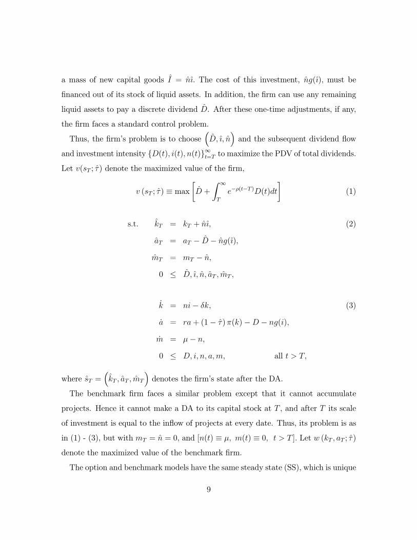
a mass of new capital goods = The cost of this investment, () must be

financed out of its stock of liquid assets. In addition, the firm can use any remaining

liquid assets to pay a discrete dividend . After these one-time adjustments, if any,

the firm faces a standard control problem.

Thus, the firm’s problem is to choose³

´and the subsequent dividend flow

and investment intensity {() () ()}∞= to maximize the PDV of total dividends.Let ( ; ) denote the maximized value of the firm,

( ; ) ≡ max∙ +

Z ∞

−(− )()

¸(1)

s.t. = + (2)

= − − ()

= −

0 ≤

= − (3)

= + (1− )()− − ()

= −

0 ≤ all

where =³

´denotes the firm’s state after the DA.

The benchmark firm faces a similar problem except that it cannot accumulate

projects. Hence it cannot make a DA to its capital stock at , and after its scale

of investment is equal to the inflow of projects at every date. Thus, its problem is as

in (1) - (3), but with = = 0 and [() ≡ () ≡ 0 ] Let ( ; )

denote the maximized value of the benchmark firm.

The option and benchmark models have the same steady state (SS), which is unique

9

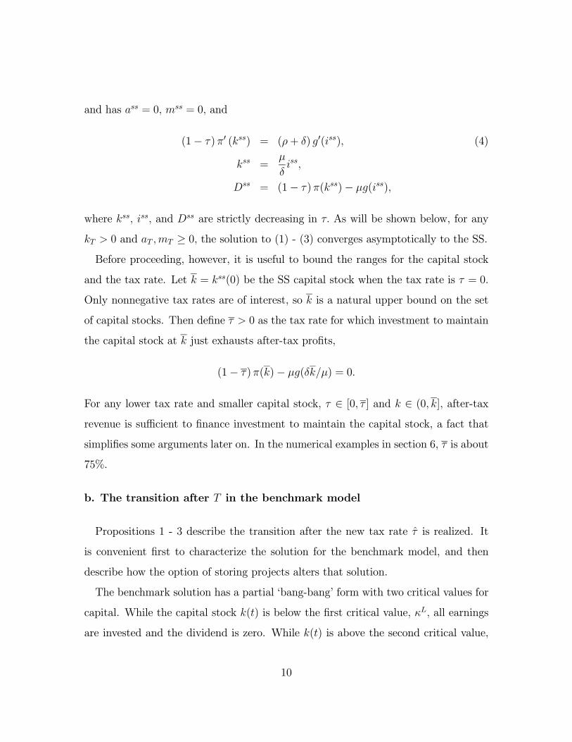
and has = 0 = 0 and

(1− )0 () = (+ ) 0() (4)

=

= (1− )()− ()

where and are strictly decreasing in As will be shown below, for any

0 and ≥ 0 the solution to (1) - (3) converges asymptotically to the SS.Before proceeding, however, it is useful to bound the ranges for the capital stock

and the tax rate. Let = (0) be the SS capital stock when the tax rate is = 0

Only nonnegative tax rates are of interest, so is a natural upper bound on the set

of capital stocks. Then define 0 as the tax rate for which investment to maintain

the capital stock at just exhausts after-tax profits,

(1− )()− () = 0

For any lower tax rate and smaller capital stock, ∈ [0 ] and ∈ (0 ] after-taxrevenue is sufficient to finance investment to maintain the capital stock, a fact that

simplifies some arguments later on. In the numerical examples in section 6, is about

75%.

b. The transition after in the benchmark model

Propositions 1 - 3 describe the transition after the new tax rate is realized. It

is convenient first to characterize the solution for the benchmark model, and then

describe how the option of storing projects alters that solution.

The benchmark solution has a partial ‘bang-bang’ form with two critical values for

capital. While the capital stock () is below the first critical value, all earnings

are invested and the dividend is zero. While () is above the second critical value,

10

all earnings are paid out as dividends and there is no investment. While () is

between the two critical values, both investment and the dividend are positive.

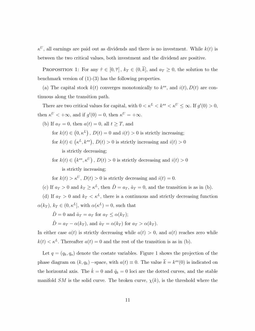
Proposition 1: For any ∈ [0 ] ∈ (0 ] and ≥ 0 the solution to thebenchmark version of (1)-(3) has the following properties.

(a) The capital stock () converges monotonically to and ()() are con-

tinuous along the transition path.

There are two critical values for capital, with 0 ≤ ∞ If 0(0) 0,

then +∞ and if 0(0) = 0 then = +∞

(b) If = 0 then () = 0 all ≥ and

for () ∈ ¡0 ¢ () = 0 and () 0 is strictly increasing;

for () ∈ ¡ ¢, () 0 is strictly increasing and () 0

is strictly decreasing;

for () ∈ ¡ ¢ () 0 is strictly decreasing and () 0

is strictly increasing;

for () () 0 is strictly decreasing and () = 0

(c) If 0 and ≥ then = = 0 and the transition is as in (b).

(d) If 0 and there is a continuous and strictly decreasing function

( ) ∈ (0 ], with () = 0 such that

= 0 and = for ≤ ( );

= − ( ) and = ( ) for ( )

In either case () is strictly decreasing while () 0, and () reaches zero while

() Thereafter () = 0 and the rest of the transition is as in (b).

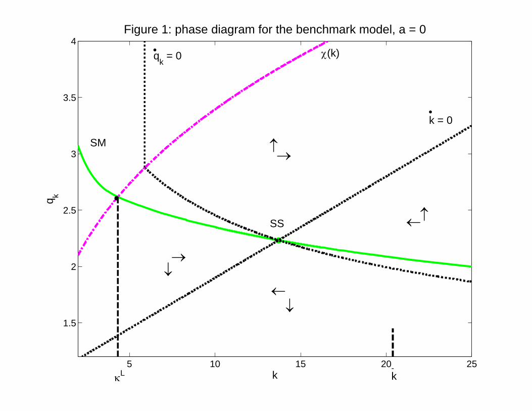
Let = ( ) denote the costate variables. Figure 1 shows the projection of the

phase diagram on ( )−space, with () ≡ 0. The value = (0) is indicated on

the horizontal axis. The = 0 and = 0 loci are the dotted curves, and the stable

manifold is the solid curve. The broken curve, () is the threshold where the

11

firm becomes cash constrained. Above that curve the firm is constrained, with 1

and = 0 Below it the firm is unconstrained, with = 1 and 0 The critical

value is defined by the intersection of and (). In this example so

the region where ∗ = 0 does not appear in the figure.

If the initial asset stock is zero, = 0 the transition is along in Figure 1, and

liquid assets are never acquired. If initial assets are positive, 0 there are two

possibilities. If ≥ the relevant portion of lies below () in the region

where = 1 Thus, the firm’s profit flow is sufficient to finance investment at the

desired rate with funds left over for a dividend. Hence the entire initial asset stock is

paid as a dividend, = and rest of the solution is unchanged.

If the firm’s profit flow is insufficient to finance investment at the desired

rate. In this case the initial dividend is less than the asset stock, 0 ≤ and

the remaining assets are used for investment. Thus, the solution involves () 0

over a finite period. Let denote the date when assets are depleted. Since =

(− ) 0 for ∈ [ ) it follows that ( ) 1 which implies ( )

c. The transition after in the option model

Next consider a firm with the option to store projects. Proposition 2 describes

a key feature of the transition: stocks of liquid assets and projects are never held

simultaneously. Thus, the DA ( ) exhausts at least one of the initial stocks, so

the subsequent transition begins with = 0 or = 0 or both, and at least one

stock is zero at every later date as well. In addition, the post-DA stock of liquid

assets can be positive only if the post-DA capital stock is less than

Proposition 2: For any ∈ [0 ] ∈ (0 ] and ≥ 0 the solution to(1) - (3) has the property that: = 0 and ()() = 0 all In addition

0 implies

12

The proof of the last claim is immediate. If ≥ the firm is not liquidity

constrained, and = 1 Hence any excess cash is paid out immediately as a dividend,

and = 0

The next result describes potential post-DA transitions in the option model. In

accord with Proposition 2, attention is limited to initial conditions with = 0

with if 0 The transitions involve two new thresholds, 0 If

the capital stock lies outside the interval£0

¤and = 0 the firm accumulates

projects. For capital stocks below 0 the firm is cash constrained, and it accumulates

projects in order to fund them later, at higher intensities, after its cash flow has

improved. For capital stocks above the firm is decumulating capital, and it

hoards projects to use later to reduce the cost of replacement investment.

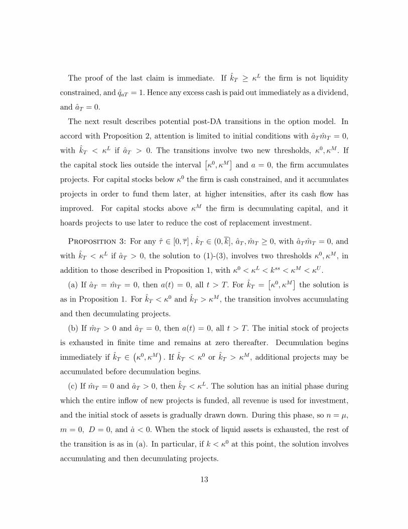
Proposition 3: For any ∈ [0 ] ∈ (0 ] ≥ 0 with = 0 and

with if 0 the solution to (1)-(3), involves two thresholds 0 in

addition to those described in Proposition 1, with 0

(a) If = = 0 then () = 0 all For =£0

¤the solution is

as in Proposition 1. For 0 and the transition involves accumulating

and then decumulating projects.

(b) If 0 and = 0 then () = 0 all The initial stock of projects

is exhausted in finite time and remains at zero thereafter. Decumulation begins

immediately if ∈¡0

¢ If 0 or additional projects may be

accumulated before decumulation begins.

(c) If = 0 and 0 then The solution has an initial phase during

which the entire inflow of new projects is funded, all revenue is used for investment,

and the initial stock of assets is gradually drawn down. During this phase, so =

= 0 = 0 and 0 When the stock of liquid assets is exhausted, the rest of

the transition is as in (a). In particular, if 0 at this point, the solution involves

accumulating and then decumulating projects.

13

If = 0 the transition in the option model is the same as in the benchmark

model for intermediate levels of the capital stock, ∈ £0 ¤ Only for capitalstocks outside this range does the firm accumulate projects after date If 0

the firm immediately starts decumulating projects if ∈£0

¤ For capital stock

outside this range, it accumlates more projects before tapping into the stock.

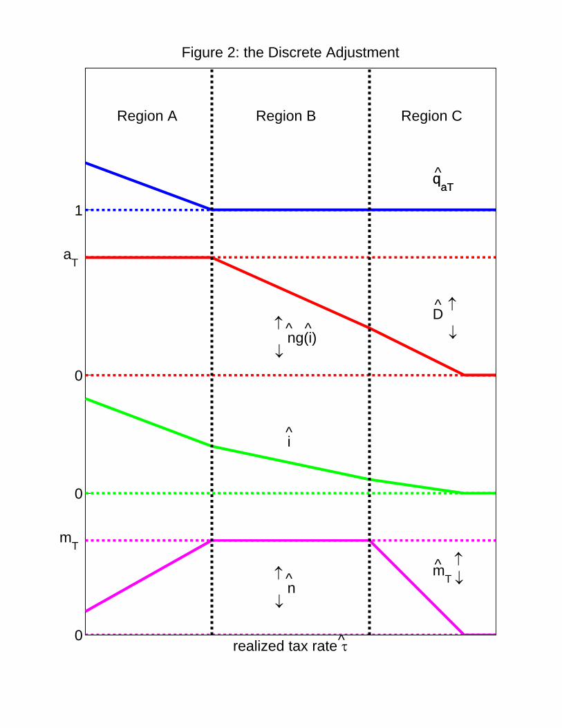
d. The DA at

The firm’s choice about the DA at depends on the realized tax rate with

lower rates producing an incentive for higher investment intensity. For fixed 0

and positive stocks of both assets, 0 Figure 2 shows, qualitatively, how

() and the initial costate value vary with Note that the description

of as low, moderate or high means relative to other values in the support of The

initial tax rate may be higher or lower than all these values.

The support of is divided into three regions. For the lowest realizations of

Region A, the firm would like to invest in the accumulated projects with a high

intensity, but it is cash constrained. In this region the DA exhausts the firm’s stock

of liquid assets, () = and some projects remain, No initial dividend is

paid, = 0 and cash is at a premium, 1 In this region is strictly increasing

in while and are strictly decreasing. After date the stock of remaining

projects is gradually used. During this period all earnings are used for investment,

and no dividend is paid. When the stock of projects is exhausted the solution lies on

() and the remaining transition is as in the benchmark model.

For higher realizations of Region B, the DA continues to use the entire stock of

projects, = but the intensity of investment declines and the firm is not cash

constrained. The excess liquid assets are paid as an initial dividend, 0 The

post-DA state lies on () and the rest of the transition is as in the benchmark

model. Since = 1 the post-DA capital stock satisfies ≥ ()

14

For even higher realizations of Region C, neither the stock of projects nor the

stock of liquid assets is exhausted by the discrete investment, and the excess assets

are paid as a dividend. That is, , = − () 0 and = 1 Indeed,

for sufficiently large, = 0 For tax rates in this region, the post-DA adjustment

starts with a stock of projects 0 which is gradually used. When the stock is

exhausted, ( ) lies on ()

Note that while the intensity of the DA is decreasing in over the entire range in

Figure 2, the scale is increasing in Region A, constant in Region B, and decreasing

in Region C. Thus, a stock of projects remains after the DA in Regions A and C. The

economic motive for holding investment options after is different in the two regions,

however. In Region A the firm is accumulating capital, but it is cash constrained.

Thus, it holds some projects back in order to finance them later, out of retained

earnings, at higher intensities. In Region C the firm is reducing its capital stock, and

it hoards projects to reduce the cost of replacement investment later on. As we will

see below, there must be positive probability of a realization in Region A, where cash

is exhausted by the DA and () 1 The firm does not accumulate excessively

large stocks of cash.

Note, too, that the firm does not hold liquid assets after date Although liq-

uid assets remain after the discrete investment in Regions B and C, they are paid

immediately as a dividend.

4. THE FIRM’S STRATEGY ON [0 )

Next consider the firm’s strategy during the time interval [0 ) Assume that when

the reform is announced at = 0 the firm has no initial stocks of liquid assets or

projects, 0 = 0 = 0, and its initial capital stock is at or below the steady state

for the old tax rate, 0 ≤ () Values for 0 near () represent mature firms,

while smaller values represent younger firms. The new tax rate , which takes effect

15

at is drawn from the known distribution () and there are no further changes

thereafter. If puts unit mass on a single point, the change is deterministic.

Since there are no initial stocks of liquid assets or projects, there can be no DA or

discrete dividend at = 0 Hence the firm chooses {( )}=0 to solve

max

Z

0

−()+ −E [(( ); )] s.t. (3), (5)

where the expectation uses . The necessary conditions for an optimum are as before,

and the terminal conditions are

lim↑

() = E [ ()] (6)

lim↑

() ≥ E [ ()] w/ eq. if 0 =

where () = are the initial costate values for the problem in (1) - (3),

given the initial state ( ) = (( ) ( )( )) and the realized tax rate

Thus, the costate for capital approaching date before the uncertainty is resolved,

must equal its expected value ex post. The costates for liquid assets and projects

may exceed their expected ex post values if the stock is zero.

a. The period of delay

The main result of the paper is the next proposition, which states that in the option

model, uncertainty about the new tax rate always leads to a period of delay: there is

an interval of time before during which investment ceases.

Proposition 4: Suppose a tax change at 0 drawn from the distribution

is announced at = 0 Unless puts unit mass at a single point, there exists ∆ 0

such that ()() = 0 for ∈ ( −∆ )

The proof is by contradiction. Suppose the contrary. Because is convex, smooth-

ing the intensity of investment across projects reduces the total cost. Delaying some

16

projects from before until just after permits this type of smoothing. Of course,

if the uncertainty is small in magnitude, the period of delay is short. Thus, if is

large, the period of delay may not begin at = 0

Proposition 4 implies that 0 so all three conditions in (6) must hold with

equality. One important feature of the solution is clear from that fact and Figure

2: the firm’s optimal strategy before necessarily produces a positive probability

of being cash constrained when is realized. Since liquid assets are acquired before

the necessary conditions imply that is increasing on (0 ) Since (0) ≥ 1 itfollows that ( ) 1 At date the post-realization value satisfies 1 only if

the new tax rate lies in Region A. Hence (6) implies that the solution lies in Region

A–where the firm is cash constrained–with strictly positive probability.

Can delay occur in the absence of uncertainty? Yes, anticipation of a deterministic

tax decrease can induce the firm to accumulate both cash and projects. The Appendix

provides an example of this sort, with ≈ ≈ 0 an extremely convex cost function and an approximately linear profit function . The motive for delay in this example

is simply to wait and exploit projects when the tax climate is more favorable. The

assumptions on and make the profits from an incremental stock of projects almost

independent of when it is exploited, and the assumptions on and make waiting

almost costless.

5. STOCHASTIC ARRIVAL DATE

The date when a tax change will occur may also be uncertain, and in this section

the model above is extended to include uncertainty about For tractability, the

arrival is assumed to be Poisson, with arrival rate

A stochastic arrival date for the tax change does not affect the firm’s post-arrival

problem in (1)-(3) or the continuation value function (; ) Before the arrival the

17

firm’s problem, given 0 = (0 0 0) is to choose {( )}∞=0 to solve

max

Z ∞

0

−(+) {() + E [((); )]} s.t. (3), (7)

where the second term in the objective function is the post-reform continuation value,

and the extra exponential term represents the probability that the tax change has

not yet occurred.

The solution for (7) consists of {[ ] all 0} This solution con-verges asymptotically to a steady state. Let ∗() denote the steady state value for

= ( ) as a function of

Let e denote the random date when the tax change arrives. The initial condition

for the post-reform transition depends on the realization of e call it For small the initial condition is close to 0 = (0 0 0) so the transition is essentially as in

Proposition 1, with negligible initial stocks of assets and projects. For large the

initial condition for the post-arrival transition is close to ∗()

The next result has two parts. First, it shows that for 0 sufficiently small, the

firm does not accumulate stocks of liquid assets or projects, although it may adjust

its capital stock slightly. That is, ∗() = [∗() 0 0] where ∗() is close to ()

The second part is an analog of Proposition 4. It shows that unless the distribution

puts unit mass on a single point, for all is sufficiently large, the steady state stocks

of liquid assets and projects are positive, ∗() 0 and ∗() 0.

Proposition 5: (a) For all 0 sufficiently small, the steady state for (7) has

the property that ∗() = [∗() 0 0] where ∗() is close to () (b) Unless

puts unit mass at a single point, for all sufficiently large, ∗()∗() 0

18

6. EXAMPLES

The examples use the revenue and cost functions

() = () = 1+1

22

2

and the parameter values

= 1 = 070 1 = 1 2 = 15

= 010 = 1 = 004 = 003

The initial tax rate is 0 = 020, and the post-reform rate is

=

⎧⎨⎩ = 022 with probability 0.5025,

= 042 with probability 0.4975.

Thus, the tax reform could raise the tax rate by 2 or 22 percentage points, with

approximately equal probability. The reform is anticipated = 2 years in advance.

Figures 3 and 4 show the transition for a mature firm, one with a capital stock at

the steady state level for the initial tax rate, 0 = (0) Figure 3 shows the short-

run transition. Panels (a)-(d) show the capital stock, investment, and the stocks of

projects and liquid assets. For comparison, the transition in the benchmark model

(broken lines) is also displayed in panels (a) and (c). In the benchmark model the firm

lets the capital stock decline mildly over [0 ] by reducing the investment rate. At

when the uncertainty is resolved, the investment rate jumps up or down, depending on

the realization of the new tax rate, and thereafter the capital stock adjusts gradually

to its new steady state level.

In the option model the period of delay begins immediately, and investment ceases

over [0 ] The capital stock declines sharply, through depreciation, and the stock

of projects increases linearly. Liquid asset accumulation begins only about 5 months

before date and the stock of assets then grows linearly until .

19

At accumulated projects are implemented in a discrete adjustment. Interestingly,

the adjustment at is larger if is realized. If the higher tax rate is realized, the

firm chooses a lower intensity of investment. Hence the entire stock of projects can

be financed from the accumulated liquid assets, with cash left over. If is realized,

the firm chooses a higher intensity for each project and hence it is cash constrained.

The stock of liquid assets is insufficient to finance the entire stock of projects, and

some projects remain after the discrete adjustment. These are implemented over a

short interval after as cash becomes available.

Panels (e)-(h) show the marginal values of capital, projects, and cash, as well as

the dividend. The shadow values for both capital and projects jump down at = 0

since news about the tax change–an increase, and perhaps a large one–reduces the

value of capital. The marginal value of capital continues to fall over [0 ] as the

date of the tax increase draws closer. The marginal value of projects rises at the rate

, as it must while the stock is positive.

The dividend jumps up at = 0 when investment ceases, and then jumps down

to zero when liquid asset accumulation begins. The marginal value of cash remains

constant at unity while a dividend is paid, but rises at the rate − 0 over the

period when liquid assets are accumulated.

All of the marginal values jump again at with the direction and size of the jump

depending on the realization of the new tax rate. If is realized, the marginal values

of capital and projects jump down. In this case some liquid assets remain after the

discrete investment, and these are paid out as a discrete dividend at . The firm

also starts paying a flow dividend at this time, and the marginal value of liquid assets

jumps back to unity at

If is realized, the marginal values of capital and projects jump up. In this case

the firm is cash constrained at and a stock of projects remains. Until that stock is

exhausted, no dividend is paid and the marginal value of liquid assets remains above

20

unity.

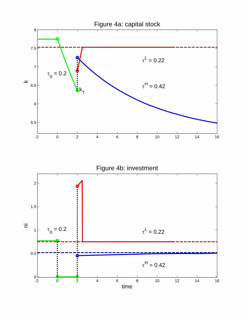
Figure 4 displays the longer run transition for the capital stock and investment, as

well as the steady state levels (dotted lines) for each realization of the new tax rate.

For the low realization, = the new steady state capital stock is only slightly

below the initial value 0 For the high realization, = the long run involves

decumulating a substantial amount of capital. In either case, the long-run adjustment

involves investing at slightly less than the new steady-state rate, producing a slow,

gradual adjustment in the capital stock.

7. CONCLUSIONS

The positive predictions of the model developed here are very stark: policy un-

certainty leads to sharp swings in investment, as the firm delays projects until the

uncertainty is resolved.

To incorporate this model of firm-level investment into a macro model, it would

be useful to let stored projects depreciate. There are two interpretations: that the

market changes, making the investment less profitable, or that a rival firm gets access

to the project and exploits it. If depreciation rates vary across projects, those with

high depreciation rates are less storable. Thus, for a policy reform with a given level

of uncertainty, projects with depreciation rates below a certain threshold would be

stored, while those above the threshold would be exploited immediately.

In highly competitive sectors, presumably the ‘depreciation’ due to rivals is greater,

making delay less feasible. Thus, highly competitive sectors should behave more

like the benchmark model, and sectors with more products that are more strongly

differentiated should behave more like the options model.

The welfare implications in a macroeconomic setting are less clear. In the model

here, the decline in investment during the period of delay is largely offset by a boom

after the uncertainty is resolved. But the same is true in many models of investment

21

over the business cycle, so the welfare costs here might be similar to the costs of

cyclical fluctuations.

[To be added: The value of the firm is a weighted sum of the values of the installed

capital, liquid assets, and stored projects that it holds. The model describes the mar-

ginal values of these three stocks, and the changes in firm valuation that accompany

delay might provide a useful signal about when delay is occurring.]

22

REFERENCES

[1] Arellano, Cristina, Yan Bai, and Patrick Kehoe. 2011. Financial markets and fluc-

tuations in uncertainty, Research Dept. Staff Report, Federal Reserve Bank of

Minneapolis.

[2] Baker, Scott, Nicholas Bloom, and Steve Davis. 2011. Measuring economic policy

uncertainty, working paper, Stanford University.

[3] Baldwin, Carliss Y. , and Richard F. Meyer. 1979. Liquidity preference under un-

certainty: A model of dynamic investment in illiquid opportunities, Journal of

Financial Economics, 7: 347-374.

[4] Bernanke, Ben S. 1983. Irreversibility, uncertainty, and cyclical investment, Quarterly

Journal of Economics, 98: 85-106.

[5] Bloom, Nicholas. 2009. The impact of uncertainty shocks, Econometrica, 77: 623-685.

[6] Bloom, Nicholas, Max Floetotto, and Nir Jaimovich. 2010. Really uncertain business

cycles, working paper, Stanford University.

[7] Cukierman, Alex. 1980. The effects of uncertainty on investment under risk neutrality

with endogenous information, Journal of Political Economy, 88: 462-475.

[8] Dixit, Avinash K., and Robert S. Pindyck. 1994. Investment under Uncertainty, MIT

Press.

[9] Fernandez-Villaverde, Jesus, Pablo Guerron-Quintana, Keith Kuester, and Juan

Rubio-Ramırez. 2011. Fiscal volatility shocks and economic activity, working

paper, University of Pennsylvania.

[10] Hopenhayn, Hugo A. and Marıa E. Muniagurria. 1996. Policy variability and eco-

nomic growth, Review of Economic Studies, 63: 611-625.

23

[11] Jovanovic, Boyan. 2009. Investment options and the business cycle, Journal of Eco-

nomic Theory.

[12] Julio, Brandon, and Youngsuk Yook. 2012. Political uncertainty and corporate in-

vestment cycles, Journal of Finance, February.

[13] Kamien, Morton I. and Nancy L. Schwartz. 1991. Dynamic Optimization: the calculus

of variations and optimal control in economics and management, second edition,

Amsterdam, North Holland.

[14] Lee, Junghoon. 2012. Does an increase in idiosyncratic volatility cause a recession,

working paper, University of Chicago.

[15] McGrattan, Ellen R. 2011. Capital taxation during the U.S. Great Depression, Staff

Report 451, Federal Reserve Bank of Minneapolis.

[16] McDonald, Robert and Daniel Siegel. 1986. The value of waiting to invest, Quarterly

Journal of Economics, 101(4): 707-728.

[17] Pastor, Lubos, and Pietro Veronesi. Political uncertainty and risk premia, Journal of

Finance, forthcoming.

[18] Seierstad, Atle and Knut Sydsaeter. 1977. Sufficient conditions in optimal control

theory, International Economic Review, 18: 367-391.

[19] Stokey, Nancy L. 2008. The Economics of Inaction: Stochastic Control Models with

Fixed Costs, Princeton University Press.

24

APPENDIX A: PROOFS OF PROPOSITIONS

Let = ( ) denote the costates for the problem in (1)-(3). The discrete

adjustment³

´satisfies2

1 ≤ w/ eq. if 0 (8)

≤ 0() w/ eq. if 0

≤ + () w/ eq. if 0

where () () and () are the costate values at date after is realized.

Thereafter the solution satisfies

1 ≤ w/ eq. if 0 (9)

≤ 0() w/ eq. if 0

≤ + () w/ eq. if 0 all

= (+ ) − (1− )0() (10)

≤ (− ) w/ eq. if 0

≤ w/ eq. if 0 all

and the transversality conditions lim→∞ −()() = 0 =

For the benchmark model, = the solution satisfies the first line in (8) and the

first and second lines in (2)-(3) and (9)-(10), and does not appear. Call this the

benchmark system.

Proof of Proposition 1: The solution { ≥ } satisfies thebenchmark system. Clearly (4) is the steady state, where the assumptions on and

ensure it is unique.

2See Kamien and Schwartz (1991) or Seierstad and Sydsaeter (1977) for a detailed discussion.

25

Suppose = 0 and conjecture the solution has () ≡ 0 Then satisfy

≤ 0() w/ eq. if 0 (11)

= (1− )()− () all ≥ (12)

Use (11) and (12) to define () by

£0−1(())

¤ ≡ (1− )()

For any , the intensity satisfying 0() = () is just sufficient to absorb all of

after-tax earnings. The function is strictly increasing, with (0) = 0(0) and the

threshold () divides ( )−space into two regions.Above the threshold the firm is cash constrained. In this region the dividend is

zero and cash is at a premium, = 0 and 1. The investment intensity, call it

∗( ) is determined by (12), so it is strictly increasing in and independent of

and (11) determines

Below the threshold the firm is not cash constrained, so 0 and = 1 In this

region the investment intensity is determined by (11), so it is strictly increasing in

and independent of and the dividend is determined by (12).

Hence the intensity isoquants in ( ) space are L-shaped, with kinks on the

( ()) threshold. If 0(0) 0 there is a second threshold, the horizontal line where

= 0(0) Below this threshold ∗ = 0 and above it ∗ 0

The locus where = 0 satisfies ∗( ) = , so it is upward sloping, hitting the

vertical axis at = 0(0) For ∈ [0 ] and 0 ∈ (0 ) the = 0 locus lies in theregion where 0 below () The locus where = 0 satisfies

(+ ) 0 [∗( )] = (1− )0()

so it is downward sloping in the region where ∗ 0 and vertical in the regions

where = 0 and ∗ = 0

26

The stable manifold, call it slopes downward, and for any ∈ (0 ] thereis unique value 0 for which the system converges to the steady state. The

critical values are defined by the points where cuts the () and

0(0) thresholds. Along intensity ∗ increases with (as falls) for

it decreases with for ∈ ¡ ¢ and it is constant at ∗ = 0 for ≥ The

dividend is = 0 for ≤ and increases with for

To verify that the conjecture () ≡ 0 is correct, it suffices to show that ≤ −If 0 then = 1 and = 0. If = 0, then so and ∗ are

increasing, and is decreasing. Since = 0(∗) it follows that 0

If 0 and ≥ then for = and = 0 the rest of the solution is as

above.

For 0 and solutions can be constructed as follows. Choose any

point ( ) on with use (12) with = 0 to determine ∗ and calculate

= 0(∗) 1 Construct trajectories for ( ) by running the relevant

ODEs in (3) and (10) backward in time, with = − 0 and 0(∗) = The

restriction ≥ 1 limits the length of the extension. The terminal pairs ( ( ))for the longest extensions define the function

Varying the length of the backward extension traces out a one-dimensional fam-

ily of initial conditions ( ) and varying the initial point on gives a two-

dimensional family. Lower initial values for on have higher initial values for

allowing longer extensions. Hence is a continuous, decreasing function, with

()→ 0 as ↑ .For 0 ≤ ( ) the initial dividend is = 0 and the transition begins with

= and 1 The solution follows a constructed trajectory until assets are

exhausted. This occurs while , and thereafter the solution follows For

( ) the initial dividend is = − ( ) and the transition begins with

= ( ) and = 1 ¥

27

Proof of Proposition 2: For the first claim it suffices to show that 0

implies = 0 Fix and suppose 0

If ( +)( +) = 0 for ∈ (0∆) then ( +) 0 which implies ()

In this region lies below (·; ) so ( +) ≡ 1 and consequently ( +) ≡ 0Hence the solution requires = 0

If ( + )( + ) 0 for ∈ (0∆) then the second and third lines in (9) holdwith equality over ( +∆) Differentiate them to get two equations involving

=

+

000

=

+

000 −

By hypothesis 0 so the third line in (10) holds with equality, and if 0 the

second line also holds with equality, so

( + ) 0 − (1− )0 = 00 (13)

[0 − ] = 00

0 + = (1− )0

and hence

(1− )0 = 0 +

Suppose this condition holds at . It continues to hold on ( +∆) if and only if

(1− )00 =h00 +

³0 −

´i (14)

The term in brackets on the right is positive, and the second line in (13) implies

≥ 0 Since 00 0 (14) holds only if ≤ 0 which implies () The rest of

the argument is as before.

The same argument shows that () 0 implies () = 0 for any

28

Finally, suppose ≥ and let 0 denote the solution for = 0 For 0

increasing the dividend by ∆ = and using 0 for the rest of the solution satisfies

all of the conditions for an optimum. ¥

Proof of Proposition 3: (a) Suppose = = 0 The solution for the option

model coincides with the solution to the benchmark model if and only if ≤

all

In the region where 1 we have 0 and

= [− 0]

so

=

+

00

0

0 −

In this region 0 and 0 Since the investment intensity is determined by

the cash flow constraint, 0 and the required condition may fail if the growth in

intensity is rapid. Define 0 as the threshold below which on

In the region where 0 and = 1

= 0()− () and 0() =

Hence

= 00 =

so the required condition holds if It also holds in some region above but

may fail for sufficiently large. It may also fail in the region where = 0 Define

as the threshold above which on

(b) Solutions with 0 can be constructed as follows. Choose 0 let

( ) = ( 0 0), and let ( ) be the associated costate values on the SM.

Construct the solution for ( ) by running the ODEs

= − (15)

29

= −

=

∙+ − (1− )0

0

¸ (16)

=

backward in time, with () = 0, all

If ≤ , then = 0 and ( ) satisfy

() =

=(1− )()

()

=

0()

where () ≡ − ()0() is strictly increasing. To verify that ≥ 1 and ≤ − note that with time running forward, is increasing and is decreasing.

Hence () and are increasing, so is falling. Since ≥ 1 on the SM, both of therequired condition holds.

By definition of the thresholds, if 0 or the solution for = 0 has

( + ) for small 0 Hence the same is true for 0 sufficiently small.

If ∈¡0

¢ the solution for = 0 has () = all and = [− 0]

with ≤ Suppose 0 is small. Then the solution requires a lower initial

value for a lower intensity, and ( + ) for small 0

To verify that = − 0 along the constructed trajectory, recall that =

on the SM. For any fixed ,

(()) ≤ (1− )() = ()

where () denotes the intensity on the SM. Hence it suffices to show that ()

When the stock of projects is exhausted, the constructed trajectory meets the SM,

so = (). Before then, is increasing along the constructed trajectory, and

() is decreasing along the SM. Hence the required condition holds for all

30

If ∈ [ ) then = 1 and 0 While 0 both the second and third

lines in (9) with equality. Together they determine from

0()− () =

Since is increasing over time, so is Going backward in time, eventually = 0

While 0 the requirement 0() = determines Specifically, (16) implies

= =

000 −

= + − (1− )0

0= 00

Combine these conditions to get

(1− )0() = 0 [+ − (0 − )]

Evidently the term in brackets is positive. Differentiate w.r.t. to get

(1− )00 =©00 [+ − (0 − )]− 0

¡00 − 0+ 2

¢ª

Since are known, and = − this equation determines The dividend is

the residual from the cash constraint,

= (1− )()− ()

To verify that = − 0 along the constructed trajectory, recall that = on

the SM. Along the constructed trajectory, and are increasing and is falling,

and the trajectory meets the SM when the stock of projects is exhausted.

There are no solutions of this type with ≥

Varying and the length of the trajectory traces out a two-dimensional manifold

of potential initial conditions for

(c) If 0 then the solution in Proposition 1 is also a solution for the option

model if at the date +∆ when liquid assets are exhausted, the capital stock satisfies

31

( +∆) ≥ 0 This happens if is not too far below 0 Otherwise, the firm is still

cash constrained after the initial stock of liquid assets is exhausted, and the solution

has a second phase where projects are first accumulated and later used, as in part (a)

above. ¥

Proof of Proposition 4: Suppose to the contrary that for any ∆ 0 the

optimal policy has ()() 0, all ∈ [−∆ ) Consider the following perturbation

to the conjectured solution over ( −∆ +∆) where ∆ 0 is small. Reduce the

flow of projects by 0 over ( −∆ ) and accumulate the projects and cash. For

0 sufficiently small, this is feasible. Then increase the flow of projects by over

( +∆) and adjust the intensity on an additional group of projects of size For

each choose the intensity for this group of 2 projects as follows.

Let ( ) denote the intensity on ( −∆ ) and let () denote the intensity on

( +∆) conditional on Since ∆ is small, these intensities are approximately

constant before and after , although the latter varies with For the 2 projects use

the intensity

() =1

2[( ) + ()]

so the capital stock at ( +∆) is unaltered.

The perturbation changes the investment cost by

∆() = ∆ {2 [ ()]− [( )]− [ ()]} all

Since is strictly convex, ∆() ≤ 0 with equality if and only if () = ( ) Unless

puts unit mass at a single point, this condition must fail on a set of ’s with positive

probability. Therefore, unless puts unit mass on a single point,

≡ E {2 [ ()]− [( )]− [ ()]} 0

Since the perturbation reduces the cost of investment, at least weakly, for every

and delays the timing of expenditures, it is also feasible in the sense that it can be

financed without any additional liquid assets.

32

The cost of the delay is the foregone revenue. The perturbation changes the capital

stock by

∆( − ) ≈ − (∆− ) ( ) ∈ (0∆) ∆( + ; ) ≈ −∆( ) + [2 ()− ()]

= − (∆− ) ( ) ∈ (0∆)

where the changes after are conditional on Hence the change in revenue is

∆Π() ≈ − (1− )0∙Z ∆

0

∆( − ) +

Z ∆

0

∆( + )

¸≈ −2 (1− )0( )

Z ∆

0

(∆− )

= −∆2 (1− )0( )

The reduction in revenue is of order ∆2 while the reduction in investment costs is

of order ∆ As noted above, 0 Hence for ∆ 0 sufficiently small,

E [∆Π()−∆()] ≈ ∆ [−∆0( )−] 0

and the perturbation raises expected profits. ¥

A deterministic tax cut with delay

To construct an example where a deterministic tax change produces delay, suppose

is approximately linear in the relevant region, let 0 be close to zero, and let

≈ Let = 1, and suppose the marginal cost of investment is piecewise linear,

with 0() = 1 for 0 ≤ 1 and 0() = 2 for 1 with 2 1 = 1

We will compare the strategy of investing at the intensity = 1 on [0 ] for some

0 with the strategy of accumulating projects and cash and carrying out

the same investment at If the firm invests at the rate = 1 over [0 ] then the

increment to its capital stock over [0 ] is approximately

∆() ≈ ¡− 22

¢ ≈ ∈ [0 ]

33

Thus, ignoring discounting, the incremental profit over [0 ] is approximately

∆Π1 ≈ (1− )0∙Z

0

∆()+∆()

Z

−(−)

¸≈ (1− )0

∙1

22 +

1− −(−)

¸≈ (1− )0

1− −

The increment to the capital stock at date from this investment is ∆1( ) ≈ −

If the firm waits until date it gets no incremental profit flow over [0 ] but the

incremental capital stock at is ∆2( ) = Hence the extra capital if investment is

delayed is ∆ ≡ ∆2−∆1 = ¡1− −

¢ The extra profit flow from this increment

from onward is approximately

∆Π2 ≈ (1− )0Z ∞

∆−(− )

= (1− )0¡1− −

¢ 1

The firm chooses to delay investment if ∆Π2 ∆Π1 which holds for any tax cut,

1− 1−

Stochastic arrival date

The first order conditions for the problem in (7) are again as in (9), but the laws

of motion for the costates now include terms that pick up the expected capital gains

or losses on the assets when the tax change occurs. Thus, (10) is replaced by

= (+ ) − (1− )0() + { − E [ (; )]} (17)

≤ (− ) + { − E [ (; )]} w/ eq. if 0

≤ + { − E [ (; )]} w/ eq. if 0

where (; ) denotes the initial value of the costate for the post-reform transition,

conditional on the state and the realized tax rate and where we have used the

34

fact that (; ) ≡ (; ) =

From (3), a steady state requires

∗ = ∗ = ∗ ∗ = (1− )(∗)− (∗) + ∗ (18)

where the restriction to tax rates ∈ [0 ) implies ∗ ≤ (0) so ∗ 0 Since

∗ ∗ ∗ 0 (9) implies

∗ = 1 ∗ = 0(∗) ∗ = (∗) (19)

where () ≡ 0() − () with 0() 0 These conditions determine ∗ ∗ ∗ as

functions of ∗ Use (18) and (19) to find that at a steady state (17) requires

{E (∗; )− 0(∗)} = (+ ) 0(∗)− (1− )0(∗) (20)

{E [ (∗; )]− 1} ≤ − w/ eq. if ∗ 0

{E [ (∗; )]− (∗)} ≤ (∗) w/ eq. if ∗ 0

The three conditions in (20) determine (∗ ∗∗) Let ∗() denote the SS as a

function of

Proof of Proposition 5: (a) For = 0 the first line in (20) requires ∗ =

() Then for ∗ = ∗ = 0 the second and third lines hold with strict inequality.

Hence ∗(0) = [() 0 0]

Consider the term in braces on the left in the first line of (20),

≡ E [ (∗(0); )]− 0(∗)

If = 0, then the first line also holds for 0

Otherwise, since is strictly convex and is strictly concave, an increase in ∗

increases the RHS of the first line and decreases the LHS. Thus, if 0 an increase

in ∗ is needed to restore equality for small 0 If 0 then by the same

reasoning, a decrease in ∗ is needed to restore equality. In both cases the second

35

and third lines continue to hold for 0 sufficiently small. Hence, in these cases

∗() = [() + () 0 0] where () has the sign of

(b) Choose large, and suppose to the contrary that ∗ = 0 or ∗ = 0 or both.

Consider the initial condition 0 = ∗() and consider the following perturbation to

the strategy of choosing () = ∗() all 0

Let ∗ denote the SS intensity, and choose ∆ 0 small. Over (0∆) reduce the

flow of projects by keeping the intensity unchanged. At = ∆ the capital stock

is reduced by ∆∗ and the firm has a stock of = ∆ untapped projects and a

stock of = ∆(∗) liquid assets. Over³∆ e´ reduce the intensity of replacement

investment by ∆∗ so the capital stock remains constant. Pay the interest on

the accumulated liquid assets and the savings in replacement cost as dividends. The

EDV of the additional dividends is

∆ = ∆

∙(∗) +

∗0(∗)

¸Z ∞

0

−(+)

=

∙(∗) +

∗0(∗)

¸∆

+ (21)

These terms are positive and have order ∆

After the tax change arrives, over³e e +∆

´increase the scale of investment by

and alter the intensity for an additional projects as in the proof of Proposition 4,

so the capital stock at e +∆ is as it would have been under the original plan. Define

() and () as in the proof of Prop. 4. Conditional on the new tax rate the

perturbation to the investment cost is

∆() = ∆ {2 [ ()]− (∗)− [ ()]} all

As shown in the proof of Prop. 4, ∆() ≤ 0 with equality if and only if () = ∗

Therefore, unless puts unit mass on a single point,

(∗) ≡ E {2 [ ()]− (∗)− [ ()]} 0

36

Hence this contribution of the perturbation to the EDV of profits is

−∆ = −∆(∗)Z ∞

0

−(+)

= −(∗) ∆

+ (22)

This term is positive and has order ∆

The perturbation changes the capital stock by

∆() =

⎧⎪⎪⎪⎨⎪⎪⎪⎩−∗ ∈ (0∆) −∗∆ ∈

³∆ e´

∗h−

³e +∆´i

∈³e e +∆

´

The PDV of the change in revenues over the interval (0∆) evaluated at = 0 is

∆ = − (1− )0∗Z ∆

0

−

≈ − (1− )0∗∆2

2

which has order ∆2 The EDV of the change in revenues over³e e +∆

´also has

order ∆2 Hence both terms can be dropped.

The EDV of the change in revenue over³∆ e´ is

∆ = −∆∗ (1− )0Z ∞

∆

−(+)

≈ − (1− )0∗∆

+ (23)

This term is negative and has order ∆

Summing the components in (21)-(23) and dropping those of order higher than ∆

we find that the perturbation is profitable for ∆ sufficiently small if and only if

0 (∗) +

∗0(∗)− (∗)− (1− )0∗

The first three terms are positive, and the last is negative. But as grows without

bound, with fixed, ∗ and ∗ = ∗ converge to limiting values. Hence for

sufficiently large, the third term, which is positive, dominates the last one. ¥

37

5 10 15 20 25

1.5

2

2.5

3

3.5

4

k

q k

Figure 1: phase diagram for the benchmark model, a = 0qk = 0 (k)

k = 0

SM

SS

L -k

0

0

0

1

Figure 2: the Discrete Adjustment

^realized tax rate

Region A Region B Region C

aT

mT

qaTqaT

D

^ ^ng(i)

i

n

mT

-1 0 1 2 3 4 56.2

6.4

6.6

6.8

7

7.2

7.4

7.6

7.8

0 = 0.2

L = 0.22

H = 0.42

Figure 3a: capital stock

k

time

-1 0 1 2 3 4 50

0.5

1

1.5

2

Figure 3c: investment

ni

time

-1 0 1 2 3 4 50

0.5

1

1.5

2

Figure 3b: projects

m

mT

-1 0 1 2 3 4 50

0.2

0.4

0.6

0.8

1

1.2

Figure 3d: liquid assets

a

aT

-1 0 1 2 3 4 51.6

1.7

1.8

1.9

2

2.1

2.2Fig 3e: MV capital

qkTq k

time

0 = 0.2

L = 0.22

H = 0.42

-1 0 1 2 3 4 50

0.5

1

1.5

2

2.5

3

3.5Figure 3g: dividend

D

time

-1 0 1 2 3 4 50.15

0.2

0.25

0.3

0.35

0.4

0.45

Figure 3f: MV projects

qmT

q m

time

-1 0 1 2 3 4 51

1.001

1.002

1.003

1.004

1.005

1.006

1.007

1.008

1.009

Figure 3h: MV liquid assets

qaTq a

time

-2 0 2 4 6 8 10 12 14 16

5.5

6

6.5

7

7.5

8

0 = 0.2

L = 0.22

H = 0.42

Figure 4a: capital stockk

kT

-2 0 2 4 6 8 10 12 14 160

0.5

1

1.5

2

0 = 0.2 L = 0.22

H = 0.42

Figure 4b: investment

ni

time