Arithmetic dynamics

Dragos Ghioca and Thomas Tucker

A simple question

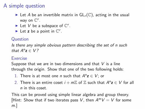
I Let A be an invertible matrix in GLr (C), acting in the usualway on Cr .

I Let V be a subspace of Cr .I Let z be a point in Cr .

QuestionIs there any simple obvious pattern describing the set of n suchthat Anz ∈ V?

ExerciseSuppose that we are in two dimensions and that V is a linethrough the origin. Show that one of the two following holds:

1. There is at most one n such that Anz ∈ V ; or

2. There is an entire coset i + mZ of Z such that Anz ∈ V for alln in this coset.

This can be proved using simple linear algebra and group theory.[Hint: Show that if two iterates pass V , then AmV = V for somem.]

One more very simple example

Let’s just do one very simple example.

Example

Let A =

(−2 0

0 2

)and let s =

(11

). Let V be the subspace

consisting of all vectors of the form

(x

−x

). Then Ans ∈ V if

and only if n is odd, i.e. if n ∈ 1 + 2Z.

Note that A2 sends V to itself, so once you get some Ai s ∈ V , youmust get Ai+2ks ∈ V for any k (this is why you do not get any“singleton cosets” here).

Other examples

The case of lines through the origin is particularly simple, bothbecause the proof is obvious and because the formulation is sosimple: Things are not quite so simple in general. For example,when V is a line that does not pass through the origin, it is easy tosee that you can have s 6= t with Asz ∈ V and Atz ∈ V withoutgetting an entire coset, just by drawing a line.

But in the case of lines not passing through the origin, once youhave a large finite number of n such that Anz ∈ V , you must havean entire coset of such n. (In fact, there is an explicit bound onthat number, 61, due to Beukers-Schlickewei, which is likelynowhere near sharp.)

Linear recurrence sequences

The first results on the problem above were proved by Skolem, inthe context of closely related questions on linear recurrencesequences.We call {an}n∈N ⊂ C a linear recurrence sequence if for somek ∈ N there exist c0, . . . , ck−1 ∈ C such that for each n ∈ N wehave

an+k = ck−1an+k−1 + · · ·+ c1an+1 + c0an.

The associated characteristic equation for this sequence is

xk − ck−1xk−1 − · · · − c1x − c0 = 0.

We let r1, . . . , rm be the distinct, nonzero roots of the abovecharacteristic equation. Then there exist polynomialsf1, . . . , fm ∈ C[z ] (deg(fi ) is less than the order of multiplicity ofthe root ri ) such that for each n ∈ N we have

an = f1(n)rn1 + · · ·+ fm(n)rn

m. (1)

It’s easy to see formula (1) in the case m = k (i.e., all roots of thecharacteristic equation are distinct and nonzero). In that case thepolynomials fi are simply constants which we find by solving thek-by-k system of equations obtained from verifying the aboveformula for n = 1, . . . , k. Then, note that since each λi is a root ofxk − ck−1x

k−1 − · · · − c1x − c0 = 0, we have

λn+ki = cn+k−1λ

n+k−1i + · · ·+ c1λ

n+1i + c0λ

n

so (1) then continues to hold by induction. When λi is a doubleroot, then it also satisfies the derivative of(xn)(xk − ck−1x

k−1 − · · · − c1x − c0), so we have

(n+k)λn+ki = (n+k−1)cn+k−1λ

n+k−1i +· · ·+(n+1)c1λ

n+1i +c0λ

n,

which allows relations involving linear polynomials fi (n) to bepreserved by induction. The same reasoning applies to higher orderfi (n) when λi is a higher-order root.

Example

Let {an}n≥1 be the sequence defined by

a1 = −3; a2 = 0; a3 = −15 and

an+3 = 3an+1 − 2an.

The characteristic equation is

x3 − 3x + 2 = 0

whose roots are r1 = 1 (twice) and r2 = −2. Thus we search for aformula

an = (An + B)rn1 + Crn

2 ,

with A,B,C ∈ C. We find that A = −3, B = 2 and C = 1; so

an = −3n + 2 + (−2)n.

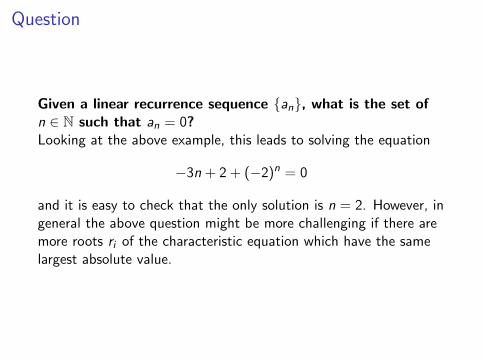
Question

Given a linear recurrence sequence {an}, what is the set ofn ∈ N such that an = 0?Looking at the above example, this leads to solving the equation

−3n + 2 + (−2)n = 0

and it is easy to check that the only solution is n = 2. However, ingeneral the above question might be more challenging if there aremore roots ri of the characteristic equation which have the samelargest absolute value.

“Analytic functions”

Assume that each ri is a positive real number; then

F (x) :=m∑

i=1

fi (x)r xi

is a real analytic function. So, the question is when F (x) = 0(especially, for which values x which are positive integers). Stillthis doesn’t solve the problem, but it provides the motivation forthe Skolem’s method which will solve the problem. Rather thanwork over R, we will work over “p-adic fields” where:

1. The integers Z are actually in the unit disc (very differentfrom R or C.)

2. Non-zero convergent power series have finitely many zeros (asover R or C).

Then writing F (x) as a p-adic analytic power series will solve ourproblem completely.

p-adic valuation

Let p be a prime number. For each nonzero integer n we denote byvp(n) the exponent of p in n. We extend the function vp to allnonzero rational numbers a/b by letting vp(a/b) = vp(a)− vp(b).Example: v3(7/9) = −2

p-adic norm

For a prime number p and any nonzero rational number x we let

|x |p := p−vp(x)

be the p-adic norm of x . It’s easy to show that

|x + y |p ≤ max{|x |p, |y |p}

with equality if |x |p 6= |y |p. This allows us to define a metric on Qby letting the distance between two rational numbers x and y be|x − y |p.

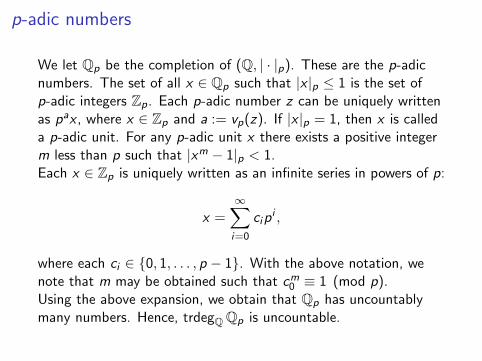
p-adic numbers

We let Qp be the completion of (Q, | · |p). These are the p-adicnumbers. The set of all x ∈ Qp such that |x |p ≤ 1 is the set ofp-adic integers Zp. Each p-adic number z can be uniquely writtenas pax , where x ∈ Zp and a := vp(z). If |x |p = 1, then x is calleda p-adic unit. For any p-adic unit x there exists a positive integerm less than p such that |xm − 1|p < 1.Each x ∈ Zp is uniquely written as an infinite series in powers of p:

x =∞∑i=0

cipi ,

where each ci ∈ {0, 1, . . . , p − 1}. With the above notation, wenote that m may be obtained such that cm

0 ≡ 1 (mod p).Using the above expansion, we obtain that Qp has uncountablymany numbers. Hence, trdegQ Qp is uncountable.

p-adic analytic functions

Let a ∈ Qp and r > 0 be a positive real number. We say thatf : Qp −→ Qp is a p-adic analytic function on the open ballD(a; r) if it has a power series expansion

∞∑i=0

ci (x − a)i

which is convergent for all x ∈ D(a; r).

TheoremIf f is p-adic analytic on D(a; r), then its zeros cannot accumulateat a point inside D(a; r).

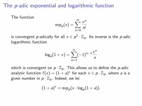
The p-adic exponential and logarithmic function

The function

expp(x) =∞∑

n=0

xn

n!

is convergent p-adically for all x ∈ p2 · Zp. Its inverse is the p-adiclogarithmic function

logp(1 + x) =∞∑

n=1

(−1)n−1 xn

n

which is convergent on p · Zp. This allows us to define the p-adicanalytic function f (x) = (1 + a)x for each x ∈ p · Zp, where a is agiven number in p · Zp. Indeed, we let

(1 + a)x = expp(x · logp(1 + a)).

What is our goal?

For a given finite set S of nonzero complex numbers, we want tofind a prime number p and an embedding σ of the finitelygenerated field Q(S) into Qp such that for each x ∈ S , we haveσ(x) ∈ Zp.Why?We want this since then we can choose the set S be the finite setcontaining all (nonzero) coefficients of the polynomials fi and allri ’s, and also the inverses of all of these numbers. We also chooseS to contain the inverses of these numbers so that the embeddingwe found actually sends each number of S into a p-adic unit.

So, assume we obtained the above embedding. We can let then Mbe a positive integer such that for each i = 1, . . . ,m we have

|rMi − 1|p < 1.

Then for each j = 0, . . . ,M − 1, the function

Fj(x) :=m∑

i=1

fi (Mx + j)rMx+ji =

m∑i=1

fi (Mx + j)r ji ·

(rMi

)x

is a p-adic analytic function. Hence we split the sequence {an}into M subsequences and for each one of them we found aparametrization by a p-adic analytic function. Using the Theoremon zeros of p-adic analytic functions we conclude that the set ofintegers n for which an = 0 is a finite union of arithmeticprogressions, where (for us) a single number is the arithmeticprogression of ratio 0.

An example of embedding

Say that we want to embed into a suitable Zp the following set ofnumbers S :=

{251 , π, e,

3√

7, i}. We proceed one number from S

at a time.As long as p does not divide 51, we can always embed 2

51 into Zp;so all prime numbers p work except for 3 and 17.For the numbers π and e, we can easily find two algebraicallyindependent (over Q) elements u and v of Qp (for any prime p)since trdegQ Qp is infinite. Then we can find an isomorphismσ : Q(π, e) −→ Q(u, v) such that σ(π) = u and σ(e) = v .It’s a bit harder to find a suitable prime p for the desiredembedding of 3

√7 and of i .

Embedding of algebraic numbers into Qp

If i ∈ Zp then it has a p-adic expansion

i = c0 + c1 · p + · · · .

In particular, c20 + 1 ≡ 0 (mod p). So we are searching for prime

numbers p such that the congruence equation

x2 ≡ −1 (mod p)

is solvable in integers. Immediately this yields that p ≡ 1 (mod 4).Conversely, if p ≡ 1 (mod 4), then we can solve for c0, c1, . . . sothat i ∈ Zp. For proving this we use Hensel’s Lemma.

Hensel’s Lemma

TheoremLet f ∈ Z[x ], let x0 ∈ Z such that f (x0) ≡ 0 (mod p) andf ′(x0) 6= 0 (mod p). Then there exists z0 ∈ Zp such thatz0 − x0 ∈ p · Zp and f (z0) = 0.

The proof constructs progressively better approximations of z0, i.e.,we construct {xn}n≥1 such that for each n ≥ 1 we have

xn ≡ xn−1 (mod pn) and f (xn) ≡ 0 (mod pn+1).

Then z0 is the limit (in Zp) of the above sequence {xn}.

So, going back to finding a suitable prime number p so that both iand 3

√7 embed into Zp, we deal now with the latter.

If 3√

7 = c0 + c1p + · · · ∈ Zp, then

c30 ≡ 7 (mod p).

Furthermore, as long as p is neither 3 nor 7, then Hensel’s Lemmacan be applied to show that 3

√7 ∈ Zp. So all we need is to find a

prime number p such that the congruence equation

x3 ≡ 7 (mod p)

is solvable. If p ≡ 2 (mod 3), then any integer is a perfect cubemodulo p.

Conclusion of the example

So, as long as p /∈ {3, 7, 17} and in addition,

p ≡ 1 (mod 4) and p ≡ 2 (mod 3)

then each of the numbers from S ={

251 , π, e,

3√

7, i}

can beembedded into Zp. Next we have to show that this can be donesimultaneously.Yes, we can do this since for each distinct x , y ∈ S ,Q(x) ∩Q(y) = Q (the intersection being taken in C).

Skolem-Mahler-Lech Theorem

The above always works, we can always embed any arithmeticsequence in Qp. So we obtain the following.

TheoremLet (an)

∞n=1 be a linear recurrence sequence. Then the set of

positive integers n such that an = 0 is a finite union of arithmeticsequences.

An arithmetic sequence is a set of integers of the form`, `+ M, `+ 2M, ..... We allow M = 0, which gives a “singletonsequence”. The M here is the power we must raise elements to sothat we can take their p-adic logarithm.

Algebraic dynamics

For any algebraic variety X endowed with a self-map Φ, we denoteby Φn the n-th iterate of Φ (for each n ∈ N). For any α ∈ X wedenote by OrbΦ(α) the orbit of α under Φ, i.e., the set of allΦn(α) for nonnegative integers n.Example. X = A1, Φ(x) = x2 + 1 and α = 0. Then

OrbΦ(α) = {0, 1, 2, 5, 26, 676, . . . }

If OrbΦ(α) is finite, then we call the point α preperiodic.

One geometric reformulation of Skolem-Mahler-Lech

The following comes directly from the proof of theSkolem-Mahler-Lech theorem.

TheoremLet Φ : CN −→ CN be a linear map, let z ∈ CN , and let V be asubvariety of CN . Then the set of n such that Φn(z) ∈ V is afinite union of arithmetic sequences.

Recall that a subvariety of CN is simply the zero set of a set ofn-variable polynomials with coefficients in C. In this context weusually write CN as AN(C).

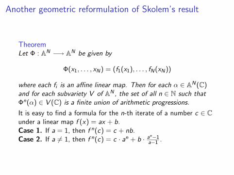
Another geometric reformulation of Skolem’s result

TheoremLet Φ : AN −→ AN be given by

Φ(x1, . . . , xN) = (f1(x1), . . . , fN(xN))

where each fi is an affine linear map. Then for each α ∈ AN(C)and for each subvariety V of AN , the set of all n ∈ N such thatΦn(α) ∈ V (C) is a finite union of arithmetic progressions.

It is easy to find a formula for the n-th iterate of a number c ∈ Cunder a linear map f (x) = ax + b.Case 1. If a = 1, then f n(c) = c + nb.Case 2. If a 6= 1, then f n(c) = c · an + b · an−1

a−1 .

Now, a point (γ1, . . . , γN) in AN lies on a given affine subvariety Vif for each F (x1, . . . , xN) in the vanishing ideal of V , we haveF (γ1, . . . , γN) = 0.Using the fact that we have explicit formulas for the n-th iterate ofa number under a linear map, we immediately get that the equation

F (f n1 (α1), . . . , f

nN (αn)) = 0

translates into an equation of the form

m∑i=1

gi (n)rni = 0

for some polynomials gi and some numbers ri . Then Skolem’sTheorem finishes the problem. Note that during our proof weactually obtain a p-adic parametrization of the orbit of α under Φ.

Extension to automorphisms of AN

The above morphisms given by the coordinatewise action of alinear map are automorphisms of AN . However there are morecomplicated automorphisms of AN ; for example

Φ(x , y) = (y + x2,−2x)

is an automorphism of A2 with inverse

Ψ(x , y) = (−y/2, x − y2/4).

It’s still possible to find suitable p-adic parametrizations of theorbit of any point in AN under an automorphism Φ of AN . Thekey is that the determinant of the Jacobian of an automorphism ofAN is a nonzero constant.

Preliminaries

So, we have an automorphism of AN given by

Φ(x1, . . . , xN) := (F1, . . . ,FN)

where each Fi ∈ C[x1, . . . , xN ]. We choose a suitable primenumber p such that

(1) each coefficient of each Fi embeds into Zp; and

(2) under this embedding, the Jacobian of Φ is mapped to ap-adic unit.

Strategy – informal

Suppose that there is a prime p and a modulus M such that foreach congruence class i modulo M, there is a p-adic analytic map

θi : Zp −→ A(Qp) such that θi (k) = Φi+Mk(z).

For each polynomial G that vanishes on V , we have that

G ◦ θi : Zp −→ Zp

is a one variable analytic power series. Thus G ◦ θi either has atmost finitely many zeroes or is itself identically zero. Since forn = Mk + i , we have An(z) ∈ V if and only if G ◦ θi (k) = 0 for allG vanishing on V , we see that either

I Φi+Mk(z) ∈ V at most for finitely many k (these give“singleton”cosets); or

I Φi+Mk(z) ∈ V for all k (these give infinite cosets).

Construction of the p-adic analytic functions

LemmaLet Φ := (F1, . . . ,FN) : ZN

p −→ ZNp be a surjective polynomial

map whose Jacobian has constant determinant which is a p-adicunit. Then there exists a positive integer k such thatΦk := (H1, . . . ,HN) has the following two properties:

(i) Hi (z1, . . . , zN) ≡ zi (mod p) for all z1, . . . , zN ∈ Zp; and

(ii) for each z := (z1, . . . , zN) ∈ ZNp , the Jacobian of Φk at z is of

the form IN + p ·Mz , for some matrix Mz with entries in Zp.

The first part is easy since Φ induces a bijective action on FNp , and

thus a suitable power Φj induces the identity map on FNp . Now, we

let m be the order of the reduction of J(Φj , ·) modulo p seen as anelement of GLN(Fp). We have

J(Φjm, z) = J(Φj , z) · J(Φj ,Φj(z)) · · · J(Φj ,Φj(m−1)(z)).

By our choice of j , we have J(Φj ,Φji (z)) ≡ J(Φj , z) (mod p) forall i ; hence k = j ·m works for the above Lemma.

Construction of the p-adic analytic functions (continued)

LemmaLet Ψ := (H1, . . . ,HN) : ZN

p −→ ZNp be a polynomial map

satisfying:

(i) Hi (z1, . . . , zN) ≡ zi (mod p) for all z1, . . . , zN ∈ Zp; and

(ii) for each z := (z1, . . . , zN) ∈ ZNp , the Jacobian of Ψ at z is of

the form IN + p ·Mz , for some matrix Mz with entries in Zp.

Then for each given point z0 ∈ ZNp , there exist

g1, . . . , gN ∈ Qp[[x ]] which are analytic on Zp such that

(1) (g1(0), g2(0) · · · , gN(0)) = z0; and

(2) gi (z + 1) = Hi (g1(z), · · · , gN(z)) for each i = 1, . . . ,N andfor each z ∈ Zp.

The above lemma shows that

Ψn(z0) = (g1(n), g2(n), · · · gN(n)),

which is the desired p-adic analytic parametrization for our orbit.

Generalized Skolem-Mahler-Lech

The above method can be generalized to any unramified self-mapon any quasiprojective variety. A map is said to be unramified ifthe Jacobian never vanishes.

TheoremLet X be a quasiprojective variety defined over C, let Φ be anunramified endomorphism of X , let α ∈ X (C) and let V be asubvariety of X . Then the set of all n ∈ N such thatΦn(α) ∈ V (C) is a finite union of arithmetic progressions.

Examples: endomorphisms of group varieties, automorphisms ofK3 surfaces.... What about when a map is not unramified?

Why do constant Jacobians help?

Here’s the (admittedly oversimplified) idea...If the Jacobian is constant, one can take its p-adic logarithm at allbut finitely many p, after raising to a sufficient power. Consider

A =

(4 00 7

)Then we can take p-adic logarithms of suitable powers of A at allprimes but 4 and 7. For example, at 3 we obtain

An =

(exp3(n log3 4) 0

0 exp3(n log3 7)

)Something more sophisticated will work whenever the Jacobian isnon-vanishing.

p-adic dynamics in one variable

Let f (x) ∈ Z. Choose p prime to the degree of f such that all thenonzero coefficients of f are p-adic units.Then the p-adic dynamics of f are surprisingly simple.First look at the level of “residue classes modulo p”.Within each periodic residue class, there are three possiblebehaviors: indifferent, attracting, and superattracting Each givesdifferent sorts of functions. (Note: there are no “repelling periodicpoints” so no chaos.)

Analytic uniformization of the orbit of a single variableanalytic function

DefinitionLet p be a prime. Let U = pZp. Let f : U → U be a function suchthat

f (t) =∑i≥0

ci ti ∈ Qp[[t]],

with |c0|p < 1, |c1|p = 1, and |ci |p ≤ 1 for all i ≥ 1. Then we sayU is a quasiperiodicity disk for f .

The conditions on f in the above Definition mean precisely that fis p-adic analytic and maps U bijectively onto U. U is called aquasiperiodicity domain of f (in the sense of Rivera-Letelier).In particular, the preperiodic points of f in U are in fact periodic.

The indifferent case – theorem

Although quasiperiodicity domains are complicated in general, ifwe put in one extra assumption – that c1 is congruent to 1 modulop, we get the following very simple theorem.

Theorem(Rivera-Letelier, BGT) Pick z ∈ U as above. There exists abijective analytic map σ : pZp −→ U such that

f k(z) = σ(σ−1(z) + k).

In other words, z moves around as if being translated!Note that σ depends on z .

Example of constructing the parametrization in theindifferent case

Say that f (z) = λz , where |λ− 1|p < 1. We want to find afunction u(z) such that f (u(z)) = u(z + 1). We let µ = log(λ)and u(z) = exp(µz) would work.

Example of the indifferent case

Let f (x) = 7 + 3x + 4x2 − 5x4 + 2x5 and consider the orbit of 0under f (x).Then for p = 7, D(0; 1) is a domain of quasiperiodicity for f (x)and therefore there exists a 7-adic uniformization map u(x) asabove.Furthermore, since f 6(x) has the linear term 729 ≡ 1 (mod 7), weget that f 6(x) is conjugated through a 7-adic analytic mapu : Z7 −→ Z7 to x 7→ x + 1, i.e.,

f (u(x)) = u(x + 1).

So, for each n ∈ N we have

f n(0) = u(n + α0),

where u(α0) = 0.

Example of the attracting case

Let f (x) = 3x + 4x2 − 5x4 + 2x5 and consider the orbit of 1 underf (x). 7-adically we are in the previous scenario, but what about3-adically?One can prove the existence of a point y ∈ 3 · Z3 such thatf (y) = y ; this is Hensel’s Lemma again. Then we can show thatf (x) is conjugated through a 3-adic analytic function u(x) tox 7→ 3x , i.e.,

f (u(x)) = u(3x).

Hence for each n ∈ N, we have

f n(1) = u(3n · α0),

where u(α0) = 1.

Example of the superattracting case

Let f (x) = 4x2− 5x4 + 2x5 and consider the orbit of 3 under f (x).It is immediate to see that the orbit converges to 0 in the 3-adictopology.One can prove that f (x) is conjugated through a 3-adic analyticfunction u(x) to x 7→ x2, i.e.,

f (u(x)) = u(x2).

Hence for each n ∈ N, we have

f n(3) = u(α2n

0

),

where u(α0) = 3.

Parametrization at an attracting fixed point – theorem

Let f (z) = a0 + a1z + a2z2 + · · · ∈ Zp[[z ]] be a nonconstant power

series with |a0|p, |a1|p < 1. Then there is a point |y |p < 1 suchthat f (y) = y , and limn→∞ f n(z) = y for all |z |p < 1. In otherwords, an attracting point. . Write λ = f ′(y); then |λ|p < 1. Wemay change coordinates to make the fixed point 0. Let U = pZp.Suppose that λ 6= 0. Then we have

TheoremThere is a bijective analytic map σ : pZp −→ U such that

f k(z) = σ(λkσ−1(z))

for all z ∈ U.

Sketch of constructing the uniformization at an attractingpoint

We have

f (z) = λz · (1 + g(z)), where g(z) = O(z).

So, for each positive integer n we have

un(z) := λ−nf n(z) = z ·(1+g(z))(1+g(f (z))) · · · (1+g(f n−1(z))).

One can prove that {un} converges to an analytic function u andsince

λun+1 = un ◦ f

we conclude that indeed f is p-adically analytically conjugate toz 7→ λz through the function u(z).

Parametrization at a superattracting fixed point – theorem

Let f (z) = a0 + a1z + a2z2 + · · · ∈ Zp[[z ]] be a nonconstant power

series with |a0|p, |a1|p < 1. Then there is a point y ∈ pZp suchthat f (y) = y , and limn→∞ f n(z) = y for all z ∈ D(0, 1). In otherwords, an attracting point. . Write λ = f ′(y); then |λ|p < 1. Wemay change coordinates to make the fixed point 0. Let U = pZp.Suppose now that λ = 0, and let am be the first nonzerocoefficient of f . Then we have

TheoremThere is a bijective analytic map σ : pZp −→ U such that

f k(z) = σ((σ−1(z))m

k).

for all z ∈ U.

Sketch of constructing the uniformization at asuperattracting point

After conjugating by a suitable map z 7→ cz we may assume that

f (z) = zm · (1 + g(z)), where g(z) = O(z).

We compute then for each positive integer n:

f n(z) = zmn ·(1+g(z))mn−1 ·(1+g(f (z)))m

n−2 · · · (1+g(f n−1(z))).

One can prove that the function

z 7→∑n≥0

log(1 + g(f n(z)))

mn+1

converges uniformly to another function h(z).

Sketch of constructing the uniformization at asuperattracting point (continued)

Sinceh(f (z)) = mh(z)− log(1 + g(z))

we get that

log

(f (z)

zm

)= mh(z)− h(f (z))

and letting u(z) = z · exp(h(z)) yields

u(f (z)) = u(z)m.

Indifferent is good

In the above, the indifferent U are much more complicated,but...they do give us p-adic analytic uniformization.Look at the underlying maps:

1. Indifferent: we have f k(z) looks like z + k (obviously p-adicanalytic in k).

2. Attracting: we have f k(z) looks like λkz , where |λ|p < 1, sowe cannot take a logarithm, so not p-adic analytic.

3. Superattracting, we have f k(z) looks like (zmk), also not

analytic in k when |z |p < 1.

One final note: the translation for indifferents comes from “takinga second log”. You start with λkz , but taking logp makes thisk logp λ+ z . Then rescale to get 1.

The Dynamical Mordell-Lang Conjecture

Conjecture

Let X be a quasiprojective variety defined over C, let Φ be anendomorphism of X , let α ∈ X (C) and let V be a subvariety of X .Then the set of all n ∈ N such that Φn(α) ∈ V (C) is a finite unionof arithmetic progressions.

We’ve seen that the result holds for all unramified maps. The keylies in finding a suitable prime p and a p-adic parametrization ofthe orbit. This works when the orbit ends up in an indifferent cyclemodulo p.When we deal with an attracting cycle modulo p, the methodmight work as long as we have a single multiplier, i.e., theJacobian of Φ at a point of the orbit is a multiple λ of the identitymatrix, where |λ|p < 1.Also the superattracting case works under restricted hypothesis.

Why Mordell-Lang?

Assume X = AN , α = (1, . . . , 1) and

Φ(x1, . . . , xN) = (a1x1, . . . , aNxN)

for some nonzero numbers ai . Then the above Conjecture reducesto the problem of understanding what is the intersection betweenan affine subvariety V and a cyclic multiplicative group Γ spannedby (a1, . . . , aN). This is a special case of a Theorem of Laurent.

Laurent’s Theorem

For each field K , Gm(K ) = (K ∗, ·) is the set of its nonzeronumbers, with the usual multiplication operation.

TheoremLet F ∈ C[x1, . . . , xN ] and let Γ be a finitely generated subgroup ofGN

m. Then the set of all γ ∈ Γ such that F (γ) = 0 is a finite unionof cosets of subgroups of Γ.

One can reduce to the case F is a linear polynomial, but still theproblem remains difficult. For example, Laurent’s Theorem impliesthat there are only finitely many positive integers m and n suchthat

3m − 2n = 1.

This is the case since the curve x − y = 1 contains no positivedimensional algebraic subgroup of G2

m.

3m − 2n = 1

Such diophantine exponential equations are difficult since theyinvolve more than 1 variable. There are some obvious solutions:m = n = 1 and (m, n) = (2, 3). Are there any other solutions?No.But what about the equation

3m − 2n = 115?

Are there any other solutions besides m = 5 and n = 7?

The beginnings

Laurent’s Theorem is a special case of the classical Mordell-LangConjecture. On the other hand, everything started with Mordell’sConjecture 83 years ago.Essentially, Mordell’s Conjecture asks that a curve which is notsufficiently simple (i.e., its genus is larger than 1) it cannot haveinfinitely many rational points.Note that curves of genus 0 are parametrizable and thus theycontain infinitely many rational points, while curves of genus 1(which are the elliptic curves) sometimes contain infinitely manyrational points.If F (x , y) ∈ Q[x , y ] is a generic polynomial of degree larger than 3,then the corresponding curve has genus larger than 1. For example,

x4 + y4 = 1

has genus 3.

Already Mordell’s Conjecture implies that an equation such as

2m − 3n = 115

has finitely many solutions (m, n) ∈ N× N. Indeed, if there wereinfinitely many solutions, then there would be infinitely manysolutions (m, n) ∈ N× N with both m and n in fixed residueclasses modulo 4 (or even some larger moduli, if needed). Thisyields that for some constants c1 and c2, the equation

c1x4 − c2y

4 = 115

would contain infinitely many solutions (x , y) ∈ Q×Q. If thegenus of the above curve is larger than 1 this contradicts Mordell’sconjecture.

Mordell’s Conjecture

Mordell’s conjecture was proven by Faltings:

TheoremLet K be a number field, and C be a curve of genus greater than 1defined over K. Then C (K ) is a finite set.

Lang’s generalization

One can interpret Mordell’s Conjecture as follows: we view thecurve C embedded into its Jacobian J (which is an abelian varietyof dimension equal to the genus of C ). Then finding C (K ) reducesto finding the intersection between the curve C (inside J) with thefinitely generated group J(K ) of K -rational points of J.Mordell’s Conjecture predicts that C (K ) ∩ J(K ) is finite. Langgeneralized this problem to the case of intersecting an arbitrarysubvariety X of a semiabelian variety G with a finitely generatedsubgroup of G (K ). This is called the Mordell-Lang Conjecture andit was proven by Faltings in the case G is an abelian variety, and byVojta in the general case of a semiabelian variety.

Conjecture (Mordell-Lang)

Let G be a semiabelian variety defined over C, let V ⊂ G be asubvariety, and let Γ ⊂ G (C) be a finitely generated subgroup.Then V (C) ∩ Γ is a finite union of cosets of subgroups of Γ.

The above conjecture is indeed a generalization of Mordell’sConjecture. One sees this by noting that if we assume theintersection C (K )∩ J(K ) (taken inside the Jacobian J of the curveC ) is infinite, then Mordell-Lang’s Conjecture predicts that theabove intersection contains a coset of a infinite subgroup H ofJ(K ). Since the Zariski closure of H (in J) is a (infinite) algebraicsubgroup, we conclude that C is a translate of a 1-dimensionalalgebraic subgroup of J. However, this forces C be isomorphic toan elliptic curve, which contradicts th assumption that its genus islarger than 1.

Special points and special subvarieties

In particular, the above analysis shows that if the intersection inthe Mordell-Lang problem is infinite, then the subvariety Vcontains a translate of an infinite algebraic subgroup of G .This phenomenon fits into the philosophy that only specialsubvarieties may contain a Zariski dense set of special points. Forthe Mordell-Lang Conjecture, the special points are the points ofΓ, while the special subvarieties are finite unions of translates ofalgebraic subgroups of of G . This principle of special points andspecial subvarieties is fundamental in other important conjecturesfrom arithmetic geometry, such as: Manin-Mumford, Bogomolov,Andre-Oort, Pink-Zilber.

Limitations to possible extensions of the Mordell-Langproblem

One cannot replace G by an arbitrary algebraic subgroup definedover C. For example, the Mordell-Lang principle fails in G2

a due tothe existence of infinitely many solutions to the Pell’s equation:

x2 − 2y2 = 1.

Then the plane curve C given by the above Pell’s equationcontains infinitely many points in common with the rank-2subgroup Z× Z of G2

a(C). Also, C is not a coset of 1-dimensionalalgebraic subgroup of G2

a, and thus the intersection is not a finiteunion of cosets of subgroups of Z× Z.Similarly, we cannot (naively) extend the Mordell-Lang principle inpositive characteristic. Indeed, the curve C ⊂ G2

m defined by theequation x + y = 1 over Fp(t) contains infinitely many points incommon with the cyclic subgroup Γ ⊂ G2

m generated by (t, 1− t).However, the intersection is not a finite union of cosets ofsubgroups of Γ, and also C is not a translate of a tori.

“Special points” and “special subvarieties in the DynamicalMordell-Lang Conjecture

Conjecture

Let X be a quasiprojective variety defined over C, let Φ be anendomorphism of X , let α ∈ X (C) and let V be a subvariety of X .Then the set of all n ∈ N such that Φn(α) ∈ V (C) is a finite unionof arithmetic progressions.

The special points are the points in the orbit of α under Φ, whilethe special subvarieties are the irreducible, Φ-periodic subvarietiesof X which intersect the given orbit.

A dynamical generalization

In the Mordell-Lang Conjecture, the subgroup Γ of the semiabelianvariety G can be viewed as the orbit of the identity 0 of G under afinitely generated group of translations Φ1, . . . ,Φr acting on G .Then the conclusion would be that for any subvariety V of G , theset of all (n1, . . . , nr ) ∈ Zr such that

Φn11 · · ·Φnr

r (0) ∈ X (C)

is a finite union of cosets of subgroups of Zr .It is natural to ask what happens if one replaces:

I G with an arbitrary quasiprojective variety X defined over C;

I Φ1, . . . ,Φr with arbitrary commuting endomorphisms of G ;

I 0 by any point in X (C).

Dynamical Mordell-Lang problem Let X be a quasiprojectivevariety defined over C, let V be a subvariety of X , let Φ1, . . . ,Φr

be commuting endomorphisms of X , and let α ∈ X (C). Is the setof all (n1, . . . , nr ) ∈ Nr such that Φn1

1 · · ·Φnrr (α) ∈ V (C) a finite

union of sets of the form γ + H ∩ Nr , where γ ∈ Nr and H is asubgroup of Zr?As shown by the example of the Pell’s equation the answer issometimes “NO”. It is interesting to note that the answer is also“NO” for certain commuting semigroups of linear transformationsacting on AN . But we do have a positive answer in an importantcase of linear transformations.

TheoremIf M1, . . . ,Mr are commuting matrices which are diagonalizable,then the Dynamical Mordell-Lang problem has a positive answer.

The case of linear transformationsFor the Dynamical Mordell-Lang (DML) problem, assume X = AN

and that each endomorphism Φi is linear, given by some matrixMi ; we assume MiMj = MjMi for each i and j . Then the DMLproblem for (linear) varieties V of AN reduces to finding all tuples(n1, . . . , nr ) ∈ Nr such that for a given vector α ∈ AN we have

Mn11 · · ·Mnr

r (α) ∈ V .

Since the matrices Mi commute, they share the same Jordanblocks, and thus without loss of generality we may assume they areall in Jordan form (at the expense of replacing each Mi byB−1MiB for some suitable invertible matrix B). Furthermore, wemay assume each Mi consists of a single Jordan block, i.e. thereexist strictly upper triangular matrices Ui such that

Mi = λ · IN + Ui

where λ is the common eigenvalue of the Mi ’s.

Powers of a matrixFor a matrix M := λ · IN + U where U is nilpotent, we immediatelysee that there exist polynomials f1, . . . , fN−1 such that for alln ∈ N we have

Mn = λn · IN +N−1∑i=1

fi (n) · U i .

Hence the equation

Mn11 · · ·Mnr

r (α) ∈ V

translates into a polynomial-exponential equation of severalvariables:

F (rn11 , . . . , rnm

m , n1, . . . , nm) = 0

where the ri ’s are the eigenvalues of the matrices Mi , and F is apolynomial. We’ve seen that when n1 = · · · = nm, the Skolem’smethod applies and yields a result compatible with theMordell-Lang principle. However, in the general case when the ni ’sare distinct, then we can get much more different answers.

An example

Let

M1 =

1 −1 00 1 −20 0 1

and

M2 =

1 2 00 1 40 0 1

.

Then

M1M2 = M2M1 =

1 1 −40 1 20 0 1

.

We let α = (3, 2, 1) and let V be the line given by the equationsx = 3 and z = 1. We can compute

Mm1 Mn

2 =

1 2n −m 4n(n − 1)− 4mn + m(m − 1)0 1 4n − 2m0 0 1

.

So, we have to find nonnegative integers m and n such that

4n − 2m + 4n(n − 1)− 4mn + m(m − 1) = 0.

The solutions are

m = 3k2 and n =3(k2 ± k)

2, where k ∈ N.

This doesn’t fit into the Mordell-Lang principle.

The diagonal case

However when all the matrices Mi are diagonalizable, then theabove equation is only exponential; the polynomial part appearsonly in the presence of Jordan blocks of dimension larger than 1.So, in the diagonalizable case, the DML problem reduces toLaurent’s Theorem, i.e., solving equations of the form

F (rn11 , . . . , rnm

m ) = 0

where F ∈ C[x1, . . . , xm].

The linear caseAn interesting special case for the DML problem is when X = A2,α = (x0, y0), and V is the diagonal line given by the equationx = y , and moreover Φ1(x , y) = (f (x), y) whileΦ2(x , y) = (x , g(y)) for some polynomials f and g with complexcoefficients. Then the Dynamical Mordell-Lang problem reduces toasking for which positive integers m and n we have

f m(x0) = gn(y0)?

If one of the polynomials is linear, then the answer will notnecessarily fit the Mordell-Lang principle. Indeed, if

f (x) = x + 1; g(y) = 2y ; (x0, y0) = (0, 1)

then f m(x0) = gn(y0) if and only if m = 2n. If instead g(y) = y2

and y0 = 2, then we obtain that

f m(x0) = gn(y0) if and only if m = 22n.

However, if neither f nor g is a linear polynomial we can show thatthe Mordell-Lang principle holds for lines in the affine space.

A simple version

Theorem(GTZ) Let f , g ∈ C[x ] have degree greater than 1. If the orbitOrbf (x0) intersects the orbit Orbg (y0) in infinitely many pointsthen there exist positive integers m and n such that f m = gn.

The full case of lines

TheoremIf X = AN and V ⊂ AN is a line, and for each i = 1, . . . , r , wehave

Φi (x1, . . . , xN) = (x1, . . . , xi−1, fi (xi ), xi+1, . . . , xN)

for some polynomials fi of degree larger than 1, then theDynamical Mordell-Lang problem has a positive answer.

In particular, going back to the special case: N = 2 and V is thediagonal line, we get that if the orbit Orbf (x0) intersects the orbitOrbg (y0) in infinitely many points then there exist positive integersm and n such that f m = gn. Using our method, together withadditional analytic and topological arguments, Wang proved asimilar result where the polynomials fi are replaced by finiteBlaschke products (these are endomorphisms of the complex unitdisk).

Idea of the proof

One can show that indeed the special case of the diagonal line inA2 is the general case. Assume now that x0, y0, and all coefficientsof f and g are integers. Then knowing that f m(x0) = gn(y0) forinfinitely many positive integers m and n yields that for each pairof positive integers r and s, the curve

f r (X )− g s(Y ) = 0

contains infinitely many integral points. Using Siegel’s Theorem(together with the refinements of Bilu and Tichy) one gets that f r

and g s must have very special forms. Using the recent results ofZieve who improved on the old results of Ritt on polynomialdecomposition, one derives that the only possibility is that f and gmust share a common iterate.

Siegel’s Theorem

Theorem(Siegel 1929!) If C is a plane curve defined over Q of positivegenus, or of genus 0 but with at least 3 points at infinity, then itcontains finitely many points with both coordinates integers.

Note that if f , g ∈ Q[z ] are generic polynomials of degree largerthan 2, then the curve given by the equation

f (x)− g(y) = 0

has no irreducible component which is a genus 0 curve with atmost 2 points at infinity.

All of the previous results suggest that the Mordell-Lang principleholds in the dynamical setting always for a cyclic semigroup ofendomorphisms of the ambient space, and it holds only sometimeswhen S is not cyclic.

The Dynamical Mordell-Lang Conjecture

Let X be any quasiprojective variety defined over C, and let Φ beany endomorphism of X . Then for any subvariety V ⊂ X, and forany point α ∈ X (C), the set of integers n ∈ N such thatΦn(α) ∈ V (C) is a union of at most finitely many arithmeticprogressions.

In particular, the above conjecture predicts that only periodicsubvarieties may contain a Zariski dense set of points from a givenorbit. This reformulation is in line with the principle of specialpoints and special subvarieties outlined before: this time, thespecial points are the points of the orbit, while the specialsubvarieties are the ones which are periodic.

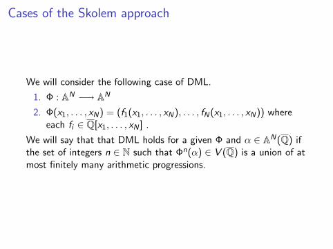
Cases of the Skolem approach

We will consider the following case of DML.

1. Φ : AN −→ AN

2. Φ(x1, . . . , xN) = (f1(x1, . . . , xN), . . . , fN(x1, . . . , xN)) whereeach fi ∈ Q[x1, . . . , xN ] .

We will say that that DML holds for a given Φ and α ∈ AN(Q) ifthe set of integers n ∈ N such that Φn(α) ∈ V (Q) is a union of atmost finitely many arithmetic progressions.

The ramification locus

The ramification locus Rϕ is defined by the vanishing of theJacobian determinant det(DΦ).We have the following: if there is a prime p such that the orbit ofα avoids the ramification locus of RΦ modulo p, then DML holdsfor Φ and α.The reason is that in this case we can construct a p-adicparametrization of the orbit of α.

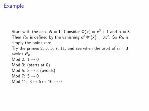
Example

Start with the case N = 1. Consider Φ(x) = x3 + 1 and α = 3.Then RΦ is defined by the vanishing of Φ′(x) = 3x2. So RΦ issimply the point zero.Try the primes 2, 3, 5, 7, 11, and see when the orbit of α = 3avoids RΦ.Mod 2: 1 7→ 0Mod 3: (starts at 0)Mod 5: 3 7→ 3 (avoids)Mod 7: 3 7→ 0Mod 11: 3 7→ 6 7→ 10 7→ 0

More examples of RΦ

Example

Φ(x1, x2) = (x21 + x2, x

51 + x3

2 ). Then RΦ is defined by thevanishing of

det

(2x1 15x4

1 3x22

)= 6x1x

22 − 5x4

1

In particular, it is a curve. More generally, we always get that RΦ

has dimension N − 1 (unless it is empty, which means Φ isunramified) when we are in dimension N.

Avoiding ramification, the birthday problem, and randommaps

Note that AN has pN points modulo p. By the “birthdayproblem”, it should therefore take about

√pN iterations for an

orbit to start to cycle modulo p.

The ramification locus RΦ has codimension 1 in AN , so it haspN−1 points modulo p. So each iterate has a 1/p chance of hittingRΦ modulo p (regardless of N).

Moral: when N is large and p is large, any given orbit probablygoes through RΦ. But...you can probably avoid ramificationmodulo some p in dimensions 1, 2, and 3.

Empirical evidence for random maps

In dimension 1, analysis predicts an average orbit length of√

p.Here is the data we obtained fixing a polynomial and starting pointα and looking at the first 1000 primes. (The chart is normalized bydividing orbit length by

√2p.) We graph against what a random

model would predict.

Empirical evidence for (failure of) ramification avoidance

See the chart below for the chance that a point passes throughramification modulo p (fixed starting point, varying maps of fixeddegree).

0.7

0.75

0.8

0.85

Pro

ba

bil

ity

Dimension 2

0

0.1

0.2

0.3

0.4

0.5

0.6

0 500 1000 1500 2000

Pro

ba

bil

ity

Prime

Dimension 1

0.5

0.55

0.6

0.65

0.7

0 500 1000 1500 2000

Pro

ba

bil

ity

Prime

0.88

0.9

0.92

0.94

0.96

0.98

1

0 50 100 150 200 250

Pro

ba

bil

ity

Prime

Dimension 3

Prime

Skolemdammerung: Twilight of the Skolem approach

Let A(p) be the chance that the orbit passes through RΦ modulo pfor a give p. Then, when N = 3, the last chart shows that

limp→∞

A(p) = 1.

But we only need to avoid ramification at a single primes, so we’reokay as long as ∏

primes p

A(p) = 0

(which it does for N = 3).When N ≥ 5, the chance of passing through ramification at aprime p goes to 1 so quickly that∏

primes p

A(p) > 0

and we have empirical evidence that there are points and maps indimension 5 where we pass through ramification at every prime p.So the Skolem approach to DML seems hopeless in general.

How bad is it when you can’t avoid ramification?

Bad: When you do not avoid ramification at p, there arecounterexamples if you replace algebraic subvariety V with p-adicanalytic subvariety V . Note that when SLM works at a prime p, itproves a result for p-adic analytic subvarieties.Good.

I We can still prove DML for algebraic subvarieties in manycases where there are p-adic analytic counterexamples.

I The counterexamples are highly transcendental, and a“dynamical transcendence theory” (suggested by Zhang)might rule these out in the algebraic case.

A special case

Consider the following special case (“split coordinates”).

I polynomials f1, . . . , fN ∈ Q[x ].

I Φ = (f1, . . . , fN) : AN −→ AN by

(f1, . . . , fN)(x1, . . . , xN) 7→ (f1(x1), . . . , fN(xN))

Here we think we can avoid ramification modulo p for infinitelymany p. (Note that we think we can “specialize” to get a proofover C, via work of Medevdev-Scanlon, Silverman,Baker-Benedetto.)

Birthday revisited

Idea: in each coordinate, should have orbit length of√

p, sothere’s only

√p/p = 1/

√p chance of passing through a given

point modulo p, so should avoid ramification mod p for a density 1set of primes.

An intersection of g sets of primes of density 1 is still density 1, sowe get lots of “ramification-avoiding” primes (so the methodworks) for (f1, . . . , fN).

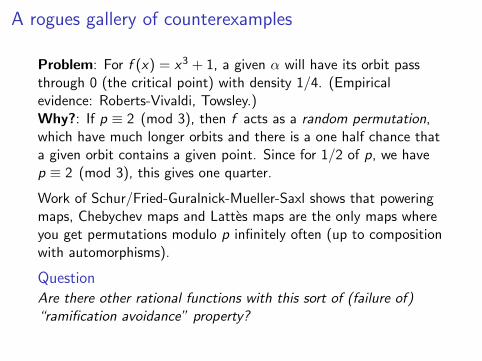
A rogues gallery of counterexamples

Problem: For f (x) = x3 + 1, a given α will have its orbit passthrough 0 (the critical point) with density 1/4. (Empiricalevidence: Roberts-Vivaldi, Towsley.)Why?: If p ≡ 2 (mod 3), then f acts as a random permutation,which have much longer orbits and there is a one half chance thata given orbit contains a given point. Since for 1/2 of p, we havep ≡ 2 (mod 3), this gives one quarter.

Work of Schur/Fried-Guralnick-Mueller-Saxl shows that poweringmaps, Chebychev maps and Lattes maps are the only maps whereyou get permutations modulo p infinitely often (up to compositionwith automorphisms).

QuestionAre there other rational functions with this sort of (failure of)“ramification avoidance” property?

Densities

Given a set S of primes, we define the density of S as

limM→∞

#{p ∈ S with p ≤ M}#{p ≤ M}

(assuming this limit exists). Here’s a sample of the type of resultthat one gets.

Theorem(Odoni-Stoll-Jones) Let f (x) = x2 + c where c 6= 0,−1,−2, andlet α ∈ Z. Suppose that the orbit of α does not pass through 0.Let T be the set of primes such that α passes through 0 modulo p.Then T has density 0.

The main tool here is the Chebotarev density theorem, which youwill treat in discussion today.

A positive result

Theorem(BGHKST) Suppose that

I polynomials f1, . . . , fN ∈ Z[x ] with fi (x) = x2 + ci .

I Φ = (f1, . . . , fN) : AN −→ AN by

(f1, . . . , fN)(x1, . . . , xN) 7→ (f1(x1), . . . , fN(xN))

Then one can avoid ramification modulo infinitely many primes pand DML holds for any subvariety, i.e for any α ∈ AN(Q) whoseorbit avoids ramification, there are infinitely many p such that theorbit of α avoids ramification modulo p.

Proof.At each ci with ci 6= 0,−1,−2, we avoid ramification with density1. We treat the cases 0,−1,−2 separately.

RemarkThere are similar results for other special polynomials.

A theorem of Lang

We deal now with another problem of “special points” and “specialvarieties”. Consider the special points be points in the affine planewith both coordinates roots of unity. In order to determine thespecial curves in A2 we search for some obvious candidates ofcurves C which would contain infinitely many points with bothcoordinates roots of unity. It’s easy to see that whenever theequation of C is

α · xmyn = 1,

for some root of unity α, then indeed C contains infinitely manypoints with both coordinates roots of unity. The interesting thingis that these are the only special ones according to the following

TheoremIf the curve C ⊂ A2 defined over C contains infinitely many pointswith both coordinates roots of unity, then the equation of C isxmyn = α, for some m, n ∈ Z and some root of unity α.

Proof of Lang’s Theorem in a special case

Assume C is a curve defined by an equation: y = g(x) for somerational function g . Furthermore, using a multiplicative translationby a root of unity, we may assume that g(1) = 1.Now, since C contains infinitely many points whose coordinates areroots of unity, we conclude that C is defined over a cyclotomicextension of Q (since, on one hand, it is defined over the infiniteextension of Q generated by all roots of unity, and on the otherhand, it is defined over a finitely generated extension of Q). So,g ∈ Q(ζm)(x) and let now {ζnk

}k an infinite sequence of primitiveroots of unity of order nk with the property that g(ζnk

) is also aroot of unity.Obviously, we may assume that n1 < n2 < · · · < nk < · · · .

Proof (continued)

For each k ∈ N let σk be an automorphism of Q such that

σk(ζnk) = e2πi/nk .

Since Q(ζm)/Q is a Galois extension, at the expense of replacingthe sequence {nk}k with a subsequence, we may assume that foreach k ∈ N, the restriction of σk on Q(ζm) is the sameautomorphism σ. Furthermore, at the expense of replacing g withgσ, we obtain that for each k ∈ N we have

σk(g(ζnk)) = g

(e2πi/nk

)is a root of unity.

Furthermore g(e2πi/nk

)∈ Q(ζm, ζnk

) ⊂ Q(ζ2mnk), which means

that there exists some dk ∈ {0, 1, . . . , 2mnk − 1} such that

g(e2πi/nk

)= e2dkπi/2mnk .

Clearly e2πi/nk → 1 as k →∞, and since g(1) = 1, we get thatalso

22dkπi/2mnk → 1 as k →∞.

At the expense of replacing g by 1/g , we may assume that

dk

mnk→ 0 as k →∞.

Complex analysis

On the other hand, using basic complex analysis, there exists somepositive real number C such that for all sufficiently large k ∈ N wehave

|g(22πi/nk

)− g(1)| ≤ C · |e2πi/nk − 1| ≤ 2Cπ

nk.

Using that g(1) = 1 and that g(e2πi/nk

)= e2dkπi/2mnk we

conclude that also

|e2dkπi/2mnk − 1| = 2 sin(dkπ/2mnk) ≤ 2Cπ

nk.

Using the inequality sin(α) > α/π for any angle α ∈ [0, π/2] allowsus to conclude that for each k ∈ N,

dk < 2Cπ.

Conclusion

By the pigeonhole principle, again at the expense of replacing {nk}with a subsequence, we may assume that dk = d for some d ∈ N,for all k ∈ N. So,

g(e2πi/nk

)= e2dπi/nk

for infinitely many nk ∈ N.Therefore g(x) = xd as desired.

The Manin-Mumford Conjecture

We note that roots of unity are precisely the torsion points forGm(C). Also, note that an equation of the form xmyn = α forsome root of unity α cuts a curve which is a torsion translate of a1-dimensional algebraic subgroup of G2

m.So, Lang’s Theorem can be reformulated (and extended) as follows.

Conjecture

If V ⊂ GNm is an irreducible subvariety which contains a Zariski

dense set of torsion points, then V is a torsion translate of analgebraic subgroup of GN

m.

The above conjecture was proven by Raynaud in a more generalform which deals with semiabelian varieties. An alternative proofto the above conjecture can be given using the results of Pila andWilkie.

An abelian variety is a projective, connected, group variety. Thesimplest example is an elliptic curve. A product of abelian varietiesis also an abelian variety. For any curve of positive genus g , itsJacobian is an abelian variety of dimension g .A semiabelian variety (over C) is an extension G of an abelianvariety A by a power of the multiplicative group, i.e., we have ashort exact sequence of group varieties (over C)

1 −→ G gm −→ G −→ A −→ 0.

Raynaud’s Theorem yields that if an irreducible subvariety V of asemiabelian variety G defined over C contains a Zariski dense setof torsion points, then V is a torsion translate of an algebraicsubgroup of G .

A dynamical reformulation

Here’s an alternative interpretation of Raynaud’s Theorem: wehave an abelian variety A and the multiplication-by-2-map Φ on A.Then the torsion points of A are the preperiodic points for Φ, whilethe torsion translates of algebraic subgroups of A are thesubvarieties which are preperiodic under the action of Φ (this partfollows from a result of Hindry).So, it is natural to ask whether it is always true for a projectivevariety X , and an endomorphism Φ of X that if a subvariety V ofX contains a Zariski dense set of preperiodic points, then V ispreperiodic itself.The above formulation is once again an instance of the philosophythat only “special” varieties may contain a Zariski dense set of“special” points.

However there are some obvious counterexamples to the aboveformulation as shown by the following example.Consider the endomorphism Φ : P1 × P1 −→ P1 × P1 be theprojectivized version of the map ϕ : A1 ×A1 −→ A1 ×A1 given byϕ(x , y) = (x2, y3). Then the diagonal subvariety contains infinitelymany preperiodic points (note that both x 7→ x2 and y 7→ y3 sharethe same set of preperiodic points) without being itself preperiodic.Same counterexample can be constructed in general: for anyabelian variety A, the endomorphism Φ : A×A −→ A×A given byΦ(x , y) = (2x , 3y) allows the diagonal subvariety of A× A containa Zariski dense set of preperiodic points (note that the torsionpoints are dense in A) without being itself preperiodic.

The Dynamical Manin-Mumford Conjecture (firstformulation)

The above problem can be easily fixed through the followingterminology.

DefinitionWe call the endomorphism Φ of the projective variety Xpolarizable if there exists some ample line bundle L and someinteger d ≥ 2 such that Φ∗(L) = d · L.

In the examples above that would force the map Φ act with thesame “weights” on both factors. So, it’s natural to formulate thefollowing conjecture (of Zhang).

Conjecture

Let Φ be a polarizable endomorphism of a projective variety Xdefined over C. If a subvariety V contains a Zariski dense set ofpreperiodic points, then V is preperiodic.

In positive characteristic, the above statement would fail due tothe presence of varieties V defined over finite fields which wouldcontain a Zariski dense set of torsion points (assuming V iscontained in an abelian variety X defined over Fp under the actionof the multiplication-by-2-map Φ) without being themselvespreperiodic under Φ.

Introduction to height functions

Before continuing with dynamical Manin-Mumford, a detour intoheights...Height functions play a crucial role in the study of diophantinegeometry. We begin with the simplest definition. Let α = a/b witha, b ∈ Z in lowest terms, that is there no p that divides both a andb. Then we define the (logarithmic) height of a/b as

h(a/b) = log max(|a|, |b|)

1. h(1) = 0.

2. h(99/100) = log 100.

3. h(0) = 0.

4. h(−23/4) = log 23.

Basic properties of height functions

For any α, β ∈ bQ, we have

1. h(αβ) ≤ h(α) + h(β).

2. h(α+ β) ≤ h(α) + h(β) + log 2.

3. For any M, there are finitely many α ∈ Q such thath(α) ≤ M.

Extending to other algebraic numbers

What if we wanted to extend this to Q?

We could intuit h(√

2) to be log 22 .

But what if we wanted to know (or at least define!) the height ofα where α is a root of x3 + 9x + 3 say? There are two ways toproceed. We will take the algebraic approach. First off, we redefineour p-adic absolute values on Q very carefully.

|p|p = p−1

In other words,|α|p = p−vp(α)

with the convention that vp(0) = ∞ so |0|p = 0.

An alternate definition of height

Why this choice of normalization?First of all, the product formula. We let M be the set{∞, 2, 3, 5, 7, 11, 13, ....}. We set | · |∞ to be the usual absolutevalue. Then for any nonzero α ∈ Q, we have the famous productformula of Weil ∏

v∈M|α|v = 1.

And crucially,

h(α) =∑v∈M

log max(|α|v , 1).

From now on, we let log+ z = log max(z , 1). Then the abovebecomes

h(α) =∑v∈M

log+ |α|v

Extending to algebraic numbers

Now, let K be a number field with [K : Q] = n. Then for anyalgebraically closed field F , there are n distinct field embeddingsσ1, . . . , σn with σi : K ↪→ F .

Each absolute value | · |v extends to the completion Qv (either Qp

or R) and then to Qv . For any α ∈ K , we may define

h(α) =1

[K : Q]

∑v∈M

∑σi :K ↪→Qv

log+ |σi (α)|v .

(Note that this does not depend on K .)

Extending to algebraic numbers, continued

h(α) =1

[K : Q]

∑v∈M

∑σi :K ↪→Qv

log+ |σi (α)|v .

We will not work explicitly with this construction very much. Let’sdo a few examples in K = Q(

√5).

1.√

5.

2.√

52 .

3. 1 +√

5.

4.√

53 .

Properties of general height functions

For any α, β ∈ Q, we have

1. h(αβ) ≤ h(α) + h(β).

2. h(α+ β) ≤ h(α) + h(β) + log 2.

3. For any M and D, there are finitely many α ∈ Q such thath(α) ≤ M and [Q(α) : Q] ≤ D. (Northcott’s theorem.) Thatis, there are finitely many points of bounded height andbounded degree.

Proof of Northcott’s theorem

Simple:

1. Let α have bounded degree and bounded height.

2. Let α1, . . . , αn be its conjugates.

3. Let

F (x) =n∏

i=1

(x − αi ).

Then the coefficients of F have bounded height from 1. and 2. ofthe previous page, since they are just symmetric polynomials in theαi

This leaves finitely many choices for each coefficient by propertiesof height functions on Q.

Points of height zero

When can a point have height zero?

Reasoning dynamically, we see that if h(α) = 0, then h(αm) = 0for all m. But all αm ∈ Q(α) so they all have bounded degree.So there must be only finitely many distinct αm, so we must haveαn = αm for some n > m, so either

1. α = 0; or

2. αn−m = 1 (α is a root of unity).

Equidistribution

By Northcott, we have the following: if limn→∞ h(αn) = 0, thenlimn→∞ degαn = ∞.

Some families where limn→∞ h(αn) = 0:

1. Primitive n-th roots of unity (αn = 1, αm 6= 1 for m < n).

2. n√

2.

3. Solutions to (xn − 1)(x − 2) + 3 (Autissier example)

Do you see a pattern?

A theorem of Bilu

Bilu proved that points with height tending to zero equidistributeon the unit circle. More specifically we have.

Theorem(Bilu) Let (αn)

∞n=1 be a nonrepeating sequence of points in Q such

that limn→∞ h(αn) = 0. Let f be a continuous bounded functionon C. Then

limn→∞

1

degαn

∑conjugates ασ

n of αn

f (ασn ) =

∫ 1

0f (e2πiz) dz

Heights in higher dimension

We can naturally extend heights to GNm by

h(α1, . . . , αN) =N∑

n=1

h(αn)

(by abuse of notation).Example

1. h(1, 3) = 0 + log 3 = log 3

2. h(4, 11) = log 4 + log 11.

3. h(i , 1) = 0.

A point in GNm has height zero if and only if it is a root of unity in

each coordinate, i.e. is a torsion point of GNmx(Q).

Bogomolov conjecture

Theorem(Zhang) Let C be an irreducible curve in G2

m such that there is aninfinite nonrepeating sequence (αn)

∞n=1 with limn→∞ h(αn) = 0.

Then C has the form x iy j = ξ, for some i , j ∈ Z and some root ofunity ξ.

This is much harder than the Serre-Ihara-Tate theorem from Lang!There are many more points with limn→∞ h(αn) = 0 than there areroots of unity.

Sketch of proof of Bogomolov a la Bilu

The proof (a sketch) is as follows: take (αn)∞n=1 with

limn→∞ h(αn) = 0 and apply maps fi ,j : (x , y) → x iy j . Then (witha bit of elementary analysis) either:

1. The (αn)∞n=1 map to a point in C , which means that the

points lie on a curve x iy j = ξ for ξ a root of unity; or

2. The (αn)∞n=1 actually equidistribute on the circle cross the

circle in G2m.

The second possibility means they do not really lie on a curve at all.

Special special case, due to Zagier

Consider the line x + y = 1. Then the only points of height zeroare (−ξ3,−ξ23), (−ξ23 ,−ξ3), (1, 0), (0, 1) (note that the last two arenot in G2

m).

Zagier explicitly calculates that for all other α ∈ G2m, we have

h(α) > 0.24.

It turns out this is not the actual lim inf, though. The lim inf isstill not known. (Just to show how difficult the Bogomolovproblem is in general.)

An interesting counterexample aside

Does it make sense to say that any family (αn)∞n=1 with

limn→∞ h(αn) = 0 is also special?

Maybe. It turns out that if f (x) = log(x − 2) (which is notcontinuous of course!), then

limn→∞

1

degαn

∑conjugates ασ

n of αn

f (ασn ) =

∫ 1

0f (e2πiz) dz

for nonrepeating sequences (αn)∞n=1 with h(αn) = 0 all n but not

necessarily if only limn→∞ h(αn) = 0 (see problem set!).

Preperiodic points and points of small canonical height

Now, let f be a polynomial of degree d with coefficients in Q.About how large is h(f (α)) compared to h(α) Let’s take a look:

f (α) = adαd + ad−1α

d−1 + · · ·+ a0.

The biggest term should dominate, so after taking logs, you shouldget about dh(α). In fact...

Height change under polynomial maps

We easily see that for all but finitely many v , we have

log+ |f (α)|v = log+ |α|dv .

(we are abusing notation a bit here, thinking of α as alreadyembedded in Qv ). At the others, we have a constant Bv such that∣∣∣log+ |f (α)|v − log+ |α|dv

∣∣∣ < Bv

(just like the proof in calculus that odd degree polynomials havereal roots). So summing up over all v , we obtain

|h(f (α))− dh(α)| < B

The canonical height

One has the Call-Silverman canonical height for a polynomial fgiven by

hf (α) = limn→∞

h(f n(α))

dn.

Why does it converge? By Tate’s famous telescoping seriesargument.

We rewrite this as

h(α) +∞∑

n=1

h(f n(α))− dh(f n−1(α))

dn.

Then |h(f n(α))−dh(f n−1(α))|dn ≤ B

dn , so the series converges.

Basic properties of canonical height

1. There is a constant M such that |h(α) = hf (α)| < M for allα ∈ Q;

2. hf (f (α)) = dhf (α) for all α ∈ Q.

3. hf (α) = 0 if and only if α is preperiodic under f .

1. gives dynamical Northcott: there are finitely many points ofbounded degree and bounded canonical height.

Then 1. and 3. give: f has only finitely many preperiodic points ofbounded degree.

Equidistribution

If we extend the height function to include the point at infinity,setting h(∞) = 0, we can define canonical heights for rationalfunctions ϕ(x) = f (x)/g(x) of degree d > 1.

All the same properties apply.

In particular, if limn→∞ h(αn) = 0, then limn→∞ degαn = ∞...soit’s not unreasonable to expect that points with height tending tozero spread out (and equidistribute) in a nice way.

Dynamical equidistribution

Any rational function has a Brolin-Lyubich measure supported onthe famous Julia set J (f ). These are the Julia sets forf (x) = x2 + c where c is as below.

(c = 0)

More on the Julia set

The Julia set J (f ) is the boundary of the filled-in Julia set ofpoints that do not escape to infinity:

{z ∈ C | limn→∞

|f n(z)| 6= ∞}

Some quick pictures

For f (x) = x2.

Julia set

Filled-in Julia set.

Julia sets and the Brolin-Lyubich measure

Let ϕ ∈ C(x) be a rational function of degree d > 1. Then theBrolin-Lyubich measure µϕ is defined as follows. Take any z thathas an infinite backwards orbit – infinitely many points such thatϕn(w) = z for some n (such points are called nonexceptional).Then define ∫

Cg dµϕ = lim

n→∞

1

dn

∑ϕn(w)=z

g(w).

Colloquially, it is the limit of the average of point masses oninverse images of z under ϕ.

The Brolin-Lyubich measure is supported on the Julia set ofϕ. (For us, that will be the definition of the Julia set for generalrational functions.)

Equidistribution revisited

Work of Baker/Hsia, Baker/Rumely, Chambert-Loir,Favre/Rivera-Letelier, and Yuan gives the following generalizationof BIlu’s result.

TheoremLet (αn)

∞n=1 be a nonrepeating sequence of algebraic points such

that limn→∞ hϕ(αn) = 0. Then∑conjugates ασ

n of α

g(ασn ) =

∫C

g dµϕ.

In other words, small points equidistribute with respect to theBrolin-Lyubich measure.

This will drive our efforts to prove dynamical Manin-Mumford.

The Dynamical Manin-Mumford Conjecture (firstformulation)

Conjecture

Let Φ be a polarizable endomorphism of a projective variety Xdefined over C. If a subvariety V contains a Zariski dense set ofpreperiodic points, then V is preperiodic.

And the Bogomolov variant.

Conjecture

Let Φ be a polarizable endomorphism of a projective variety Xdefined over Q. If a subvariety V contains a Zariski dense set ofpoints (αn)

∞n=1 with limn→∞ hΦ(αn) = 0, then V is preperiodic.

Note: we haven’t defined general canonical heights hΦ yet, but forus we will be in the split case (f1, . . . , fN) : AN −→ AN with eachfi ∈ K [x ] so hΦ(x1, . . . , xN) = hf1(x1) + . . . hfN (xN).

Bogomolov and Manin-Mumford

I Bogomolov-type results hold for small points.

I Manin-Mumford-type results hold only for preperiodic points.

I Bogomolv-type results hold only over number fields (whereheights are defined).

I Manin-Mumford-type results hold over C.

In practice, Bogomolov results seem stronger because there arevarious tricks for sending F to K where K is a number field and Fis a finitely generated ring over which our problem is defined.

Results

The above (both Manin-Mumford and Bogomolov type)conjectures hold for lines V ⊂ (P1)N under the action ofΦ := (f1, . . . , fN) where each fi ∈ Q[z ] (polynomials!) such thatdeg(f1) = · · · = deg(fN) ≥ 2.In order to prove this result one easily makes the followingreductions:

1. N = 2 (simply project on two coordinate axis at a time; eachprojection is still a line);

2. V projects dominantly to each axis (since otherwise it has toproject on one of the axis to a preperiodic point and the resultis obvious then).

3. V is the diagonal line in P1 × P1 (we achieve this by replacingg with a suitable conjugate). If V is the line given byy = σ(x) for some linear polynomial σ, then we replace gwith σ−1 ◦ g ◦ σ and obtain that both f and (the new) gshare infinitely many preperiodic points in common.

The case N = 2

In the case N = 2, we have:

I we have two maps f and g of the same degree with(f , g) : A2 −→ A2 by (f , g)(x , y) = (f (x), g(y)).

I a line L in A2.

I A nonrepeating sequence of points ((αn, βn))∞n=1 on L such

that limn→∞ hf (αn) + hg (βn) = 0.

We want to show that L is preperiodic under the action of (f , g)

The case N = 2: reduction to the diagonal

After changing coordinates, we may assume the line is thediagonal. So we have then a nonrepeating sequence of points((αn, αn))

∞n=1 such that limn→∞ hf (αn) + hg (αn) = 0. Since

hf , hg ≥ 0, this means

limn→∞

hf (αn) = limn→∞

hg (αn) = 0.

Since the αn equidistribute, they determine the Brolin-Lyubichmeasures...so we must have dµf = dµg . So J (f ) = J (g). If twopolynomials share a sequence of small points, then they have thesame Julia set.

If J (f ) = J (g), then what this means for f and g?

Classical results in complex dynamics (proven by Beardon) yieldthat the Julia set essentially governs not only the dynamics of agiven polynomial mapping, but even the polynomial itself. So,J (f ) = J (g) yields that there exists a linear isometry σ ofJ (f ) = J (g) such that g = σ ◦ f ; furthermore f ◦ σ = σd ◦ fwhere d = deg(f ) = deg(g). So (f , g)n always looks like (f n, τ f n)for some isometry τ of the Julia set.

1. If neither f nor g are conjugate to zd , then J (f ) has finitelymany isometries, and then immediately we get that thediagonal in P1 × P1 is preperiodic under the action of (f , g)since it simply moves through various a finite list ofautomorphic images of the diagonal (τx , x).

2. If f (and so, also g) is conjugate to zd , we are back toZhang’s theorem and the conclusion follows immediately.

Isometries

Which of these sets has a lot of isometries?

(c = 0)

How about rational functions?

If we try this for rational functions, ψ and ϕ, things work out thesame.

Reducing to the diagonal, we get a sequence of points that aresmall for both canonical heights, so dµϕ = dµψ.

This means the Julia sets are the same, but that is a bit weaker (itturns out) for rational functions. Two rational functions can havethe same Julia set without having the same Brolin-Lyubichmeasure.

Counterexample with Lattes maps

However, there are counterexamples when ϕ and ψ are Lattesmaps corresponding to endomorphisms of same degree of the sameCM elliptic curve.

(See diagram on board)

It does turn out these are the only counterexamples.

Why are Lattes maps good examples for counterexamples?

Lattes maps have a number of properties that make them goodcandidates for counterexamples here.

I They all have Julia sets that are equal to the whole Riemannsphere. (This has many symmetries.)

I They commute with many other maps, and these all share thesame Brolin-Lyubich measure.

I They are counterexamples to many important statements onmoduli of rational functions (Thurston rigidity, McMullenmultipier theorem, etc.).

Counterexample with CM elliptic curves

Let E be the elliptic curve given by the equation y2 = x3 − x . Theendomorphism ring of E is Z[i ]; note that

[i ](x , y) = (−x , iy).

Let ϕ be the endomorphism of E corresponding to [2 + i ] and ψ bethe endomorphism corresponding to [2− i ]. We let A = E × E andlet Ψ := (ϕ,ψ) ∈ End(A). It’s easy to see that Ψ is polarizable(here we use the fact that 2 + i and 2− i have the same norm).Also, the preperiodic points for Φ are precisely pairs of torsionpoints for E .So, the diagonal ∆ ⊂ E × E contains infinitely many preperiodicpoints for Φ, but it is not preperiodic (here we use the fact that foreach n ∈ N we have (2 + i)n 6= (2− i)n).

A simple explanation with exponential maps

Our old friend the exponential map – which helped so much withdynamical Mordell-Lang – is the villain here. Let A = E × E . Wehave a map exp (over C) that sends the tangent space at theidentity to surjectively onto C, that is

exp : TA,0 −→ A(C).

What does the Jacobian of ([2 + i ], [2− i ]) look like at the

identity?

(2 + i 0

0 2− i

). Now, exp sends the space

(xx

)onto

the diagonal in E × E ...but it obviously is not preperiodic under(2 + i 0

0 2− i

).

The Dynamical Manin-Mumford Conjecture (new version)

We believe that maybe all counterexamples to the original versionof the Dynamical Manin-Mumford Conjecture descend toendomorphisms of abelian varieties (similar to the aboveconstruction). Motivated by this we have the followingreformulation of the conjecture:

Conjecture

Let X be a projective variety, let ϕ : X −→ X be an endomorphismdefined over C with a polarization, and let Y be a subvariety of Xwhich has no component included into the singular part of X .Then Y is preperiodic under ϕ if and only if there exists a Zariskidense subset of smooth points x ∈ Y ∩ Prepϕ(X ) such that thetangent subspace of Y at x is preperiodic under the induced actionof ϕ on the Grassmanian Grdim(Y ) (TX ,x). (Here we denote byTX ,x the tangent space of X at the point x.)

Preview of coming attractions

Here is something you may be even more likely to have seen than aJulia set: Mandelbrot set.

WIth the Julia set, you fix a map, vary points and see which pointsdo not go to infinity. With a Mandelbrot set, you fix a point(namely 0), vary the map (over the family x2 + c), and see forwhich maps that point goes to infinity. The same equidistributionresults apply, and they allow us treat a whole new class ofquestions...next time!

The case of abelian varieties for the new conjecture

It is easy to check the above conjecture for all algebraic groupendomorphisms of abelian varieties. Also, the approach we hadabove for the case of lines under polynomial actions works for theabove reformulation for all lines under the coordinatewise action ofany rational maps.First note that since Φ : A −→ A is a polarizable algebraic groupendomorphism, all its preperiodic points are the torsion points of A.

Indeed, if Φn(α)− Φm(α) for some positive integers n 6= m, thenα ∈ ker(Φn−Φm). Because Φ is polarizable, Φ acts on the tangentspace of A at any point with eigenvalues of absolute value strictlylarger than 1. Therefore Φn − Φm is a finite endomorphism of A,and thus it has finite kernel, which means that α is a torsion point.If V is an irreducible subvariety of A which contains a Zariski denseset of preperiodic points for Φ, then V contains a Zariski dense setof torsion points of A and so, by Laurent’s Theorem we obtain thatV is a torsion translate of an algebraic subgroup H of A.Using the fact that the tangent subspace of V at any preperiodicpoint for Φ is preperiodic under the induced action of Φ on thetangent space of A, we get that H itself must be preperiodic underthe action of Φ.

Unlikely intersections

We return again to Lang’s Theorem:

TheoremIf the curve C ⊂ A2 defined over C contains infinitely many pointswith both coordinates roots of unity, then the equation of C isxmyn = α, for some m, n ∈ Z and some root of unity α.

Lang’s result yields (assuming C projects dominantly to both axis)that for each point (x , y) ∈ C , we have that x is a root of unity ifand only if y is a root of unity. In other words, if there is a point(x0, y0) ∈ C such that x0 is a root of unity while y0 is not a root ofunity (or vice-versa), then there exist at most finitely many points(x , y) ∈ C such that both x and y are roots of unity.Masser and Zannier proved a similar result for torsion points infibres of the Legendre family of elliptic curves. Both their resultand the above theorem of Lang fit into a more general programwhich is highlighted by the Pink-Zilber Conjecture.

The Legendre family of elliptic curves

For each λ /∈ {0, 1} we let Eλ be the elliptic curve given by theequation

y2 = x(x − 1)(x − λ)

and let Pλ := (2,√

2(2− λ)) and Qλ := (3,√

6(3− λ)).It is easy to check that P2 = (2, 0) is a 2-torsion point on E2, whileQ2 = (3,

√6) is a nontorsion point for E2. Similarly, Q3 = (3, 0) is

a 2-torsion point on E3, while P3 = (2, i√

2) is a nontorsion pointfor E3.On the other hand, one can find infinitely many λ ∈ Q such thatPλ is a torsion point for Eλ, and similarly one can find infinitelymany λ ∈ Q such that Qλ is a torsion point for Eλ.Can we find infinitely many λ ∈ C such that both Pλ and Qλ aretorsion points for Eλ?No.

The dynamical interpretation of the Masser and Zannier’sresult

For each elliptic curve Eλ we consider [2] be themultiplication-by-2-map on Eλ. Then the preperiodic points of thismap are precisely the torsion points of Eλ; hence Masser andZannier’s theorem is similar to Lang’s result on roots of unity oncurves (also recall that roots of unity are preperiodic points for thesquaring map).For example, one can find a parametrization of the C ⊂ A2 inLang’s theorem given by two algebraic functions f (z) and g(z) andthen the setting is the same as in the elliptic case: can one findinfinitely many λ ∈ C such that both f (λ) and g(λ) are roots ofunity at the same time?

The general problem

Let {Xλ} be an algebraic family of varieties parametrized byλ ∈ C. Let Pλ,Qλ ∈ Xλ be two algebraic families of points, andlet Φλ : Xλ −→ Xλ be an algebraic family of endomorphisms.Question: Under what conditions there exist infinitely manyλ ∈ C such that both Pλ and Qλ are preperiodic points for Φλ?One cannot expect to find explicit necessary and sufficientconditions satisfying the conclusion of the above question.However we note that since for each family of points Rλ oneexpects that there exist infinitely many λ ∈ C such that Rλ ispreperiodic for Φλ, then we expect that the following trichotomybe the answer to the above question:

1. Pλ is preperiodic for Φλ, for all λ; or

2. Qλ is preperiodic for Φλ, for all λ; or

3. for each λ, Pλ is preperiodic for Φλ if and only if Qλ ispreperiodic for Φλ.

A theorem of Baker and DeMarco

It is immediate to see that the conclusion in the following result fitsexactly into the trichotomy for unlikely intersections in dynamics.

TheoremLet a, b ∈ C, let d be an integer greater than 1, and letΦλ(x) = xd + λ. There exist infinitely many λ ∈ C such that botha and b are preperiodic for Φλ if and only if ad = bd .

The proof uses various techniques, from an equidistribution resulton Berkovich spaces (proven by Baker an Rumely, Favre andRivera-Letelier, and Chambert-Loir) to classical theorems incomplex dynamics and complex analysis (regarding univalentfunctions).

An example

Consider the family of polynomialsfλ(x) = x3 − λx2 + (λ2 − 1)x + λ indexed by all λ ∈ C. Leta(λ) = λ and b(λ) = λ3 − 1.Question: Are there infinitely many λ ∈ C such that both a(λ)and b(λ) are preperiodic for the same fλ?For example, λ = 0 satisfies the above conditions since then

I f0(x) = x3 − x ;

I a(0) = 0 and b(0) = −1,

and f0(0) = 0 while f0(−1) = 0.Also λ = 1 works since then

I f1(x) = x3 − x2 + 1;

I a(1) = 1 and b(1) = 0,

and f1(1) = 1 while f1(0) = 1.Are there infinitely many more such λ’s? Note that individually,there exist infinitely many λ ∈ C such that either a(λ) or b(λ) arepreperiodic for fλ (simply solve the equation f n

λ (a(λ)) = a(λ) forvarying n ∈ N).

On the other hand, λ = −1 does not work since

I f−1(x) = x3 + x2 − 1;

I a(−1) = −1 and b(−1) = −2,

and f−1(−1) = −1, while

f−1(−2) = −5; f 2−1(−2) = −101; . . . . . .

So, it’s not true that a(λ) is preperiodic exactly when b(λ) ispreperiodic, and it’s not true that b(λ) is always preperiodic underfλ. Nor it is true that a(λ) is always preperiodic, as it’s shown bythe case λ = 2. In that case,

I f2(x) = x3 − 2x2 + 3x + 2 and a(2) = 2, while

I f2(2) = 8, f 22 (2) = 410, . . . . . . .

The above two examples coupled with our conjecture suggest thatthere should only be finitely many λ ∈ C such that both a(λ) andb(λ) are preperiodic for fλ since all three conditions from thetrichotomy principle regarding unlikely intersections in dynamicsfail in this example. This follows from the next result.

TheoremLet {fλ} be any family of polynomials defined over Q of degreelarger than 1, and let a,b ∈ Q[λ]. Suppose that a and b are notpreperiodic under {fλ} in Q[λ]. If there exist infinitely many λ ∈ Qsuch that both a(λ) and b(λ) are preperiodic for fλ, then:

I for each λ ∈ Q, a(λ) is preperiodic for fλ if and only if b(λ) ispreperiodic for fλ.

Sketch of proof

The idea here, due to Baker and DeMarco, is a beautiful one.Instead of using a map to define a height on points, you use a pointto define a height on maps. Their family is fλ(x) = x2 + λ. Fixinga point a gives us a height on the parameter space {fλ}λ∈Q by

ha(λ) = hfλ(a).

Then crucially:ha(λ) = 0 if and only if a is preperiodic for fλ.

Also: One can obtain a measure corresponding to this height invarious ways and equidistribution results apply.Let’s do an example that we touched on last time.

Mandelbrot set revisited

As before, let fλ(x) = x2 + λ. Let a = 0. Then the Mandelbrot setbelow is the exact analog of the filled in Julia set. It is:

{λ ∈ C | limn→∞

|f nλ (0)| 6= ∞}

Mandelbrot set revisited

There is a natural measure one can associate to this set, theequilibrium measure (one can also obtain the measure in otherways), concentrated on the boundary. Let’s call the measure µ0.

Equidistribution

Now, let’s go back to our slightly more general setting. The familyis fλ(x) = x2 + λ. Fixing a point a gives us a height on theparameter space {fλ}λ∈Q by

ha(λ) = hfλ(a).

Theorem(Baker-DeMarco et al.) Let (λ)∞n=1 be a nonrepeating sequencesuch that limn→∞ ha(λn) = 0. Then the (λn)

∞n=1 equidistribute

with respect to dµa. (In the usual sense of weak convergence ofaverage point masses.)

In particular, when a = 0, such a family (λn)∞n=1 equidistributes on

the boundary of the Mandelbrot set.

Examples with heights

With this family again and a = 0, for which λ ∈ Q, do we haveh0(λ) = 0?

In other words, for which λ is 0 preperiodic under fλ?

We see right off that λ ∈ Z because once a denominator gets in, itwill never come out. Similarly if λ > 1, then 0 must go off toinfinity. The same if |λ| > 2. So we are just left with 0,−1,−2.We check that 0 is indeed preperiodic for these λ.

Let’s look at the Mandelbrot set again.

Idea of proof of Baker-DeMarco

Take a and b. Let ha(λ) and hb(λ) be as above. Suppose that wehave (λn)

∞n=1, be a nonrepeating sequence such that

limn→∞ ha(λn) = limn→∞ hb(λn) = 0. Then

1. (λn)∞n=1 equidistribute for both µa and µb

2. So µa = µb.

3. This forces a “special relation” between a and b (as with ourproof of Manin-Mumford, using Julia sets), namely thata2 = b2.

Notes on Baker-DeMarco

Some notes on Baker-DeMarco:

1. It gives a “Bogomolov-type” result for points of small height,not just preperiodic points.

2. It extends from Q to C via specialization.

3. The (λn)∞n=1 equidistribute for both µa and µb, so µa = µb

idea extends vastly to other situations..

4. The “special relation” a2 = b2 is difficult to prove and may behard to extend to more generality.

(One more chart on special)

Recall from earlier.

TheoremLet {fλ} be any family of polynomials defined over Q of degreelarger than 1, and let a,b ∈ Q[λ]. Suppose that a and b are notpreperiodic under {fλ} in Q[λ]. If there exist infinitely many λ ∈ Qsuch that both a(λ) and b(λ) are preperiodic for fλ, then:

I for each λ ∈ Q, a(λ) is preperiodic for fλ if and only if b(λ) ispreperiodic for fλ.

In fact, it’s enough to have a sequence of “small points”.

Proof

The same basic trickeration works but with a weaker last step.Define

ha(λ) = hfλ(a(λ))

for λ ∈ Q.

1. (λn)∞n=1 equidistribute for both µa and µb.

2. So µa = µb.

3. This forces ha = hb so the preperiodic maps are the same fora as for b.

When we can get a “special relation”

Theorem(Ghioca, Hsia, Tucker) Let d be an integer greater than 1, letcd ∈ C∗, let cd−1, . . . , c0 ∈ C[λ], and let

fλ(x) = cdxd + cd−1(λ)xd−1 + · · ·+ c1(λ)x + c0(λ).

Let a,b ∈ C[λ] such that

I deg(a) = deg(b) ≥ d ·max{deg(c0), . . . , deg(cd−1)};I a and b have the same leading coefficient.

If there exist infinitely many λ ∈ C such that both a(λ) and b(λ)are preperiodic for fλ, then a = b.

In particular, we get that a(λ) is preperiodic if and only if b(λ) ispreperiodic.

Getting the “special relation”

The special relation trick will only ever work for polynomialsbecause there you Botcher’s Uniformization Theorem, which allowsyou to choose analytic coordinate near infinity that make yourpolynomial look like a powering map (obviously can’t do this formore general rational functions).

For any (monic) polynomial g ∈ C[x ] of degree d ≥ 2, there existsa real number R ≥ 1 and an analytic map Φ : UR −→ UR , where

UR = {z ∈ C : |z | > R}

satisfying the following two conditions:

(i) Φ is univalent on UR and at ∞,

Φ(z) = z + O

(1

z

);

(ii) for all z ∈ UR we have

Φ(g(z)) = Φ(z)d .

All happy families are alike

You can actually get a result that compares different families ofmaps.

TheoremLet {fλ} and {gλ}be any family of polynomials defined over Q ofdegree larger than 1, and let a,b ∈ Q[λ]. Suppose that a is notpreperiodic under {fλ} in Q[λ] and b is not preperiodic under {gλ}in Q[λ]. If there exist infinitely many λ ∈ Q such that both a(λ)and b(λ) are preperiodic for fλ, then:

I for each λ ∈ Q, a(λ) is preperiodic for fλ if and only if b(λ) ispreperiodic for gλ.

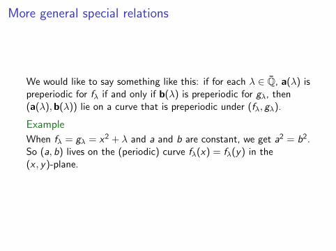
More general special relations

We would like to say something like this: if for each λ ∈ Q, a(λ) ispreperiodic for fλ if and only if b(λ) is preperiodic for gλ, then(a(λ),b(λ)) lie on a curve that is preperiodic under (fλ, gλ).

Example

When fλ = gλ = x2 + λ and a and b are constant, we get a2 = b2.So (a, b) lives on the (periodic) curve fλ(x) = fλ(y) in the(x , y)-plane.

A counterexample revisited

But in full generality, you cannot always get a dynamically specialrelation.

Example

Take the constant families of maps Lattes maps f and g where fcorresponds to multiplication by 2 + i on the elliptic curvey2 = x3 − x and g corresponds to multiplication by 2 + i . Leta(λ) = b(λ) = λ (a nonconstant family). Then there are clearlyinfinitely many λn such that λn is preperiodic for both f and g ,but there is no nice dynamically relation between a and b(although they are actually equal).

Both sides now

We would like a Bogomolov version of Masser-Zannier’s result.

Conjecture

Let E be the elliptic curve over Q(λ) given by

y2 = x(x − 1)(x − λ)

and let P,Q be two points in E (Q(λ)). Suppose that there valuesλn such that limn→∞ hEλn

(Pλn) = limn→∞ hEλn(Pλn) = 0. Then

[m]P = [n]Q in E (Q(λ)) for some m, n.

Curiously, getting the “small points” form via Pila-Wilkie seemsimpossible.Getting the “special relation” [m]P = [n]Q via equidistributionseems impossible.But maybe we can use them together.

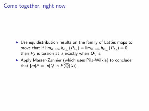
Come together, right now

I Use equidistribution results on the family of Lattes maps toprove that if limn→∞ hEλn

(Pλn) = limn→∞ hEλn(Pλn) = 0,

then Pλ is torsion at λ exactly when Qλ is.

I Apply Masser-Zannier (which uses Pila-Wilkie) to concludethat [m]P = [n]Q in E (Q(λ)).