Supplementary Material for Identifying residential neighbourhood types from settlement points in a machine learning approach

Section 1: Processing and Computational Methods

Overview of processing steps

The geometry-derived features are calculated using a moving window operation. A circular filter with a fixed radius moves across each cell of the 20 m resolution output grid. At each step, settlement points within the circular window are selected and used to calculate various features as described in the text. Each feature is stored in a separate gridded layer. The entire process is repeated for each radii.

Figure: Example processing steps to calculate geometry-derived features.

Sub-scenes within the study area

The process described above is computationally intensive given the number of radii and the large area being analysed. To improve computational efficiency of feature calculations, a recursive splitting algorithm is used to divide the study area into smaller, sub-scene areas that balances the size of the scene with the number of settlement points in the area. The smallest blocks correspond to areas with higher densities of settlement points. An example of these splits is shown in Figure 1. The smallest blocks correspond to urban areas of the provincial capital with a large number of settlement points. By adding a “halo” of cells around each sub-scene equal to the size of the processing radius, each sub-scene can be processed in parallel while avoiding edge effects in the moving window calculation.

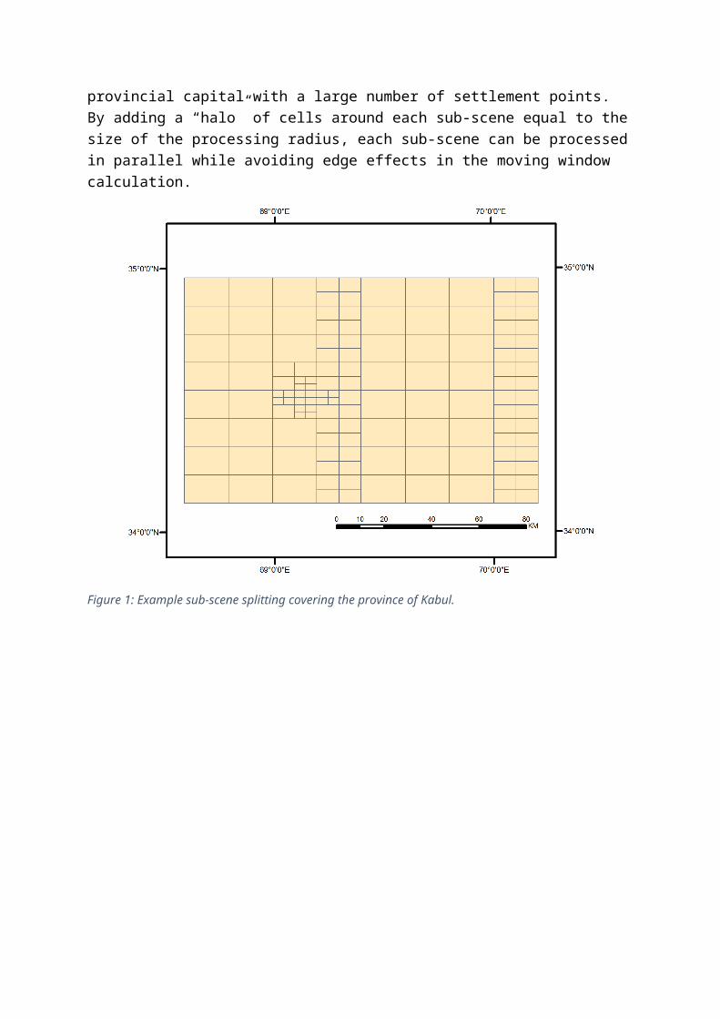
Figure 1: Example sub-scene splitting covering the province of Kabul.

Section 2: R Code demonstration of point pattern feature calculations

## Example feature calculations from settlement points# # This code demonstrates the general ideas of calculating# data features from spatial point patterns used in the# paper "Identifying residential types from settlement # points in a machine learning approach." ## Calculations use only 4 spatial scales for demonstration. # Settlement points are not actual locations.#

require(spdep)require(FNN)require(raster)

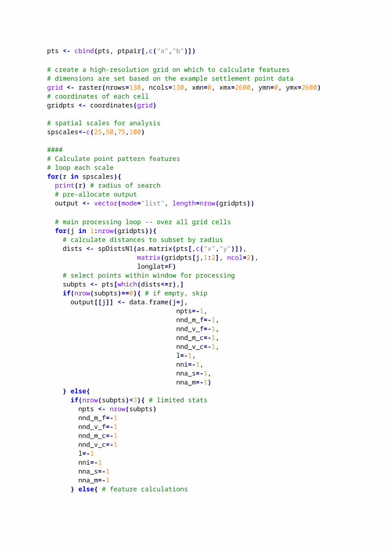
# read settlement point locations# change to your file pathsetwd("C:/Users/CHANGE/PATH/HERE/")pts <- read.csv("settlement_pts_example.csv", stringsAsFactors=F) str(pts) # uid=unique id, x/y=locations dim(pts) # n=9004 head(pts) # plot(pts$x, pts$y) # pre-calculate nearest neighbour distances and angles# used for unconstrained feature calculationskn1 <- get.knn(pts[,c("x","y")], k=1) pts$dist <- kn1$nn.dist# use neighbour pairs to find anglesptpair <- data.frame(pts[,c("x","y")], pts[kn1$nn.index, c("x","y")])names(ptpair) <- c("x1","y1","x2","y2")# make anglesptpair$dx <- ptpair$x2 - ptpair$x1ptpair$dy <- ptpair$y2 - ptpair$y1ptpair$a <- atan2(ptpair$dy, ptpair$dx) * 180/piptpair$a <- ptpair$a %% 360# bin the angles into 4 groupsptpair$b <- as.numeric(cut(ptpair$a, breaks=c(0,45,90,135,180,225,270,315,360), include.lowest=T))ptpair[ptpair$b==1 | ptpair$b==5, "b"] <- 1ptpair[ptpair$b==2 | ptpair$b==6, "b"] <- 2ptpair[ptpair$b==3 | ptpair$b==7, "b"] <- 3ptpair[ptpair$b==4 | ptpair$b==8, "b"] <- 4# merge back to the originalpts <- cbind(pts, ptpair[,c("a","b")]) # create a high-resolution grid on which to calculate features# dimensions are set based on the example settlement point datagrid <- raster(nrows=130, ncols=130, xmn=0, xmx=2600, ymn=0, ymx=2600)# coordinates of each cellgridpts <- coordinates(grid)

# spatial scales for analysisspscales<-c(25,50,75,100)

####

# Calculate point pattern features # loop each scalefor(r in spscales){ print(r) # radius of search # pre-allocate output output <- vector(mode="list", length=nrow(gridpts)) # main processing loop -- over all grid cells for(j in 1:nrow(gridpts)){ # calculate distances to subset by radius dists <- spDistsN1(as.matrix(pts[,c("x","y")]), matrix(gridpts[j,1:2], ncol=2), longlat=F) # select points within window for processing subpts <- pts[which(dists<=r),] if(nrow(subpts)==0){ # if empty, skip output[[j]] <- data.frame(j=j, npts=-1, nnd_m_f=-1, nnd_v_f=-1, nnd_m_c=-1, nnd_v_c=-1, l=-1, nni=-1, nna_s=-1, nna_m=-1) } else{ if(nrow(subpts)<3){ # limited stats npts <- nrow(subpts) nnd_m_f=-1 nnd_v_f=-1 nnd_m_c=-1 nnd_v_c=-1 l=-1 nni=-1 nna_s=-1 nna_m=-1 } else{ # feature calculations # number of points npts <- nrow(subpts) # nearest neighbour distances (unconstrained) nnd_m_f <- mean(subpts$dist) nnd_v_f <- var(subpts$dist) # nearest neighbour distances (window-constrained) kn1 <- knearneigh(as.matrix(subpts[,c("x","y")]), k=1, longlat=F) dkn1 <- nbdists(knn2nb(kn1), coords=as.matrix(subpts[,c("x","y")]), longlat=F) avgnnd <- mean(unlist(dkn1)) nnd_m_c <- avgnnd nnd_v_c <- var(unlist(dkn1)) # linearity cv <- cov(subpts) e <- eigen(cv)$values l <- (e[1]-e[2])/e[1] # nearest neighbour index nni <- avgnnd / (0.5*sqrt((pi*r^2)/nrow(subpts))) # nearest neighbour angles p <- prop.table(table(subpts$b))

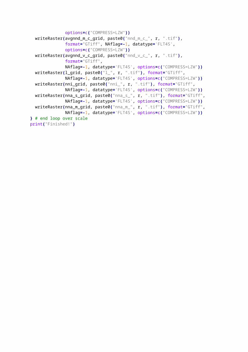
nna_s <- -sum(p*log2(p)) # shannon's entropy nna_m <- -sum(p*log2(p)) / nrow(subpts) # metric entropy } output[[j]] <- data.frame(j=j, npts, nnd_m_f, nnd_v_f, nnd_m_c, nnd_v_c, l, nni, nna_s,nna_m) } } # end loop over grid cells print(" creating rasters") # combine calculations o <- do.call(rbind.data.frame, output) # create grids npts_grid <- rasterize(gridpts, grid, field=o$npts) avgnnd_m_f_grid <- rasterize(gridpts, grid, field=o$nnd_m_f) avgnnd_v_f_grid <- rasterize(gridpts, grid, field=o$nnd_v_f) avgnnd_m_c_grid <- rasterize(gridpts, grid, field=o$nnd_m_c) avgnnd_v_c_grid <- rasterize(gridpts, grid, field=o$nnd_v_c) l_grid <- rasterize(gridpts, grid, field=o$l) nni_grid <- rasterize(gridpts, grid, field=o$nni) nna_s_grid <- rasterize(gridpts, grid, field=o$nna_s) nna_m_grid <- rasterize(gridpts, grid, field=o$nna_m) # write out for each feature writeRaster(npts_grid, paste0("npts_", r, ".tif"), format="GTiff", NAflag=-1, datatype='FLT4S', options=c("COMPRESS=LZW")) writeRaster(avgnnd_m_f_grid, paste0("nnd_m_f_", r, ".tif"), format="GTiff", NAflag=-1, datatype='FLT4S', options=c("COMPRESS=LZW")) writeRaster(avgnnd_v_f_grid, paste0("nnd_v_f_", r, ".tif"), format="GTiff", NAflag=-1, datatype='FLT4S', options=c("COMPRESS=LZW")) writeRaster(avgnnd_m_c_grid, paste0("nnd_m_c_", r, ".tif"), format="GTiff", NAflag=-1, datatype='FLT4S', options=c("COMPRESS=LZW")) writeRaster(avgnnd_v_c_grid, paste0("nnd_v_c_", r, ".tif"), format="GTiff", NAflag=-1, datatype='FLT4S', options=c("COMPRESS=LZW")) writeRaster(l_grid, paste0("l_", r, ".tif"), format="GTiff", NAflag=-1, datatype='FLT4S', options=c("COMPRESS=LZW")) writeRaster(nni_grid, paste0("nni_", r, ".tif"), format="GTiff", NAflag=-1, datatype='FLT4S', options=c("COMPRESS=LZW")) writeRaster(nna_s_grid, paste0("nna_s_", r, ".tif"), format="GTiff", NAflag=-1, datatype='FLT4S', options=c("COMPRESS=LZW")) writeRaster(nna_m_grid, paste0("nna_m_", r, ".tif"), format="GTiff", NAflag=-1, datatype='FLT4S', options=c("COMPRESS=LZW"))} # end loop over scaleprint("Finished!")

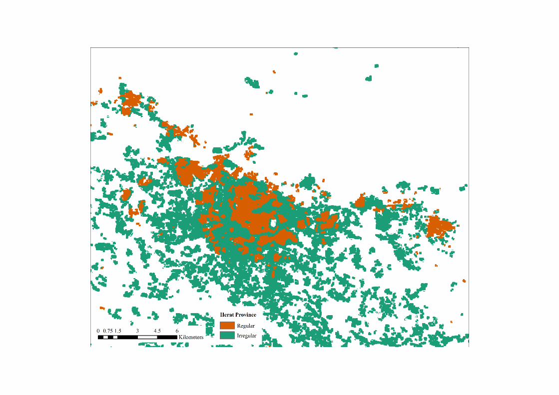
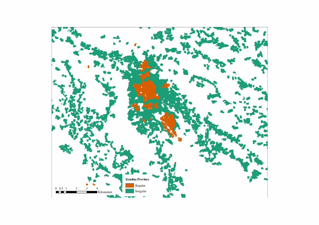
Section 3: Prediction maps for seven provincial capital areas