arthurfreitasramos - ufpe
TRANSCRIPT

Arthur Freitas Ramos
Explicit Computational Paths in Type Theory
Universidade Federal de [email protected]
http://cin.ufpe.br/~posgraduacao
Recife2018

Arthur Freitas Ramos
Explicit Computational Paths in Type Theory
Esse trabalho foi apresentado à Pós-graduação em Ciência da Computação do Centro de Informática da Universidade Federal de Pernambuco como requisito parcial para obtenção do grau de Doutor em Ciência da Computação.
Área de Concentração: Teoria da Computação
Orientadora: Anjolina Grisi de Oliveira Co-orientador: Ruy José Guerra Barreto de Queiroz
Recife2018

Catalogação na fonte Bibliotecária Monick Raquel Silvestre da S. Portes, CRB4-1217
R175e Ramos, Arthur Freitas Explicit computational paths in type theory / Arthur Freitas Ramos. – 2018.
145 f.: il., tab.
Orientadora: Anjolina Grisi de Oliveira. Tese (Doutorado) – Universidade Federal de Pernambuco. CIn, Ciência da
Computação, Recife, 2018. Inclui referências.
1. Ciência da computação. 2. Teoria da computação. I. Oliveira, AnjolinaGrisi de (orientador). II. Título.
004 CDD (23. ed.) UFPE- MEI 2018-140

Arthur Freitas Ramos
“Explicit Computational Paths in Type Theory”
Tese de Doutorado apresentada ao Programa
de Pós-Graduação em Ciência da
Computação da Universidade Federal de
Pernambuco, como requisito parcial para a
obtenção do título de Doutora em Ciência da
Computação.
Aprovado em: 17/08/2018.
_____________________________________________________
Orientadora: Profa. Anjolina Grisi de Oliveira
BANCA EXAMINADORA
______________________________________________ Prof. Frederico Luiz Gonçalves de Freitas
Centro de Informática /UFPE
______________________________________________ Prof. Edward Hermann Haeusler
Departamento de Informática / PUC/RJ
_______________________________________________ Prof. Hugo Luiz Mariano
Instituto de Matemática e Estatística / USP
_______________________________________________ Profa. Elaine Gouvêa Pimentel
Departamento de Matemática / UFRN
_______________________________________________ Prof. António Mário da Silva Marcos Florido
Departamento de Ciência de Computadores / Universidade do Porto

To my parents, Neide & Valdez, who are my role models.To my wife, Láis, for all the love and support.

ACKNOWLEDGEMENTS
This work would have not been possible without the help of many people. First, I canpoint the never-ending dedication of my parents, Neide and Valdez. Despite facing manyhardships in life, they always valued my education, supporting and encouraging my stud-ies. For this, I am eternally grateful. You are my role models and my heroes. I thankmy wife, Laís, for her patience, love and support. Without her, it would be impossible towrite this work. I also thank my advisor, Professor Ruy de Queiroz. He has been in thisjourney with me for 5 years, since the end of my undergraduate studies. I have learned agreat deal from him and he has shown me true wisdom. Last but not least, I thank Godfor giving me patience, strength and resilience every time I asked.

ABSTRACT
The current work has three main objectives. The first one is the proposal of com-putational paths as a new entity of type theory. In this proposal, we point out the factthat computational paths should be seen as the syntax counterpart of the homotopicalpaths between terms of a type. We also propose a formalization of the identity type usingcomputational paths. The second objective is the proposal of a mathematical structure fora type using computational paths. We show that using categorical semantics it is possibleto induce a groupoid structure for a type and also a higher groupoid structure, usingcomputational paths and a rewrite system. We use this groupoid structure to prove thatcomputational paths also refutes the uniqueness of identity proofs. The last objective is toformulate and prove the main concepts and building blocks of homotopy type theory. Weend this last objective with a proof of the isomorphism between the fundamental groupof the circle and the group of the integers.
Key-words: Computational paths. Homotopy type theory. Identity type. Category the-ory. Term rewrite system. Uniqueness of identity proofs.

RESUMO
O presente trabalho tem três objetivos principais. O primeiro é propor caminhos com-putacionais como uma nova entidade da teoria dos tipos. Nessa proposta, indicamos queos caminhos computacionais podem ser vistos como uma contrapartida sintática dos cam-inhos homotópicos entre termos de um mesmo tipo. Também propomos uma formalizaçãodo tipo identidade usando caminhos computacionais. O segundo objetivo é propor umaestrutura matemática para um tipo usando os caminhos computacionais. Mostramos, us-ando semântica categórica, que é possível induzir uma estrutura de grupóide de alta ordempara um tipo, utilizando os caminhos computacionais e um sistema de reescrita. Usamoso modelo de grupóide para provar que os caminhos computacionais também refutam aunicidade de provas de identidade. O último objetivo é formular e provar os principaisconceitos da teoria homotópica dos tipos utilizando caminhos. Finalizamos esse últimoobjetivo com uma prova do isomorfismo entre o grupo fundamental do círculo e o grupodos inteiros.
Palavras-chaves: Caminhos computacionais. Teoria homotópica dos tipos. Tipo iden-tidade. Teoria das categorias. Sistema de reescrita de termos. Unicidade de provas deidentidade.

LIST OF TABLES
Table 1 – Multiple semantical interpretations of a type . . . . . . . . . . . . . . . 31

LIST OF ABBREVIATIONS AND ACRONYMS
𝐼𝑑− 𝐸 identity type elimination
𝐼𝑑𝑒𝑥𝑡 − 𝐸 extensional identity type elimination
𝐼𝑑𝑒𝑥𝑡 − 𝐸𝑞 extensional identity type equality
𝐼𝑑𝑒𝑥𝑡 − 𝐹 extensional identity type formation
𝐼𝑑𝑒𝑥𝑡 − 𝐼 extensional identity type introduction
𝐼𝑑𝑖𝑛𝑡 − 𝐹 identity type formation
𝐼𝑑𝑖𝑛𝑡 − 𝐼 identity type introduction
Π − 𝐶 dependent function computation
Π − 𝐸 dependent function elimination
Π − 𝐹 dependent function formation
Π − 𝐼 dependent function introduction
Σ − 𝐸1 first dependent sum elimination
Σ − 𝐸2 second dependent sum elimination
Σ − 𝐹 dependent sum formation
Σ − 𝐼 dependent sum introduction
N− 𝐼0 zero introduction
N− 𝐼𝑠 successor induction
× − 𝐸1 first product elimination
× − 𝐸2 second product elimination
× − 𝐹 product formation
× − 𝐼 product introduction
UIP Uniquiness of Identity Proofs
ZFC Zermelo-Frankel-Choice

CONTENTS
1 INTRODUCTION . . . . . . . . . . . . . . . . . . . . . . . . . . . . 131.1 FOUNDATIONS OF MATHEMATICS AND ZFC . . . . . . . . . . . . . . 131.2 THE IDENTITY TYPE . . . . . . . . . . . . . . . . . . . . . . . . . . . . 151.3 OBJECTIVES . . . . . . . . . . . . . . . . . . . . . . . . . . . . . . . . . 161.4 STRUCTURE . . . . . . . . . . . . . . . . . . . . . . . . . . . . . . . . . 17
2 TYPE THEORY . . . . . . . . . . . . . . . . . . . . . . . . . . . . . 192.1 BASIC CONCEPTS . . . . . . . . . . . . . . . . . . . . . . . . . . . . . 202.1.1 Definitional Equality vs Propositional Equality . . . . . . . . . . . . . 202.1.2 Type Families . . . . . . . . . . . . . . . . . . . . . . . . . . . . . . . . 222.1.3 Function Type . . . . . . . . . . . . . . . . . . . . . . . . . . . . . . . . 222.1.4 Dependent Function Type(Π) . . . . . . . . . . . . . . . . . . . . . . 242.1.5 Product type (×) . . . . . . . . . . . . . . . . . . . . . . . . . . . . . . 252.1.6 Coproduct (+) . . . . . . . . . . . . . . . . . . . . . . . . . . . . . . . 262.1.7 Dependent Pair Type (Σ) . . . . . . . . . . . . . . . . . . . . . . . . . 272.1.8 Alternative Formulation for the Dependent Pair . . . . . . . . . . . . 282.1.9 The Natural Numbers . . . . . . . . . . . . . . . . . . . . . . . . . . . 292.1.10 Additional Information . . . . . . . . . . . . . . . . . . . . . . . . . . . 312.2 IDENTITY TYPE . . . . . . . . . . . . . . . . . . . . . . . . . . . . . . . 312.2.1 Formal Definition of The Identity Type . . . . . . . . . . . . . . . . . 322.2.2 Basic Constructions . . . . . . . . . . . . . . . . . . . . . . . . . . . . 332.2.3 Extensionality vs Intensionality . . . . . . . . . . . . . . . . . . . . . . 362.3 CONCLUSION . . . . . . . . . . . . . . . . . . . . . . . . . . . . . . . . 37
3 CATEGORY THEORY . . . . . . . . . . . . . . . . . . . . . . . . . 383.1 BASIC CONCEPTS . . . . . . . . . . . . . . . . . . . . . . . . . . . . . 383.1.1 Categories . . . . . . . . . . . . . . . . . . . . . . . . . . . . . . . . . . 393.1.2 Isomorphism . . . . . . . . . . . . . . . . . . . . . . . . . . . . . . . . . 413.1.3 Groupoid . . . . . . . . . . . . . . . . . . . . . . . . . . . . . . . . . . . 433.1.4 Functors . . . . . . . . . . . . . . . . . . . . . . . . . . . . . . . . . . . 433.1.5 Duality . . . . . . . . . . . . . . . . . . . . . . . . . . . . . . . . . . . . 453.1.6 Commutativity . . . . . . . . . . . . . . . . . . . . . . . . . . . . . . . 463.1.7 Product between two categories . . . . . . . . . . . . . . . . . . . . . 463.1.8 Hom and Small Categories . . . . . . . . . . . . . . . . . . . . . . . . 473.2 PRODUCT IN A CATEGORY . . . . . . . . . . . . . . . . . . . . . . . . 483.2.1 Product in Type Theory and Category Theory . . . . . . . . . . . . . 50

3.2.2 Coproduct . . . . . . . . . . . . . . . . . . . . . . . . . . . . . . . . . . 513.3 NATURAL TRANSFORMATIONS . . . . . . . . . . . . . . . . . . . . . . 513.3.1 Adjoints . . . . . . . . . . . . . . . . . . . . . . . . . . . . . . . . . . . 553.4 HIGHER CATEGORIES . . . . . . . . . . . . . . . . . . . . . . . . . . . . 573.4.1 Globular Sets . . . . . . . . . . . . . . . . . . . . . . . . . . . . . . . . 573.4.2 Horizontal Composition . . . . . . . . . . . . . . . . . . . . . . . . . . 583.4.3 Bicategories . . . . . . . . . . . . . . . . . . . . . . . . . . . . . . . . . 593.5 CONCLUSION . . . . . . . . . . . . . . . . . . . . . . . . . . . . . . . . 61
4 COMPUTATIONAL PATHS . . . . . . . . . . . . . . . . . . . . . . 624.1 INTRODUCING COMPUTATIONAL PATHS . . . . . . . . . . . . . . . . 634.1.1 Formal Definition . . . . . . . . . . . . . . . . . . . . . . . . . . . . . . 644.1.2 Equality Equations . . . . . . . . . . . . . . . . . . . . . . . . . . . . . 664.1.3 Identity Type . . . . . . . . . . . . . . . . . . . . . . . . . . . . . . . . 674.1.4 Path-based Examples . . . . . . . . . . . . . . . . . . . . . . . . . . . 684.1.4.1 Reflexivity . . . . . . . . . . . . . . . . . . . . . . . . . . . . . . . . . . . 694.1.4.2 Symmetry . . . . . . . . . . . . . . . . . . . . . . . . . . . . . . . . . . . 694.1.4.3 Transitivity . . . . . . . . . . . . . . . . . . . . . . . . . . . . . . . . . . 694.2 TERM REWRITE SYSTEM . . . . . . . . . . . . . . . . . . . . . . . . . 724.2.1 𝐿𝑁𝐷𝐸𝑄 − 𝑇𝑅𝑆 . . . . . . . . . . . . . . . . . . . . . . . . . . . . . . . 734.2.1.1 Subterm Substitution . . . . . . . . . . . . . . . . . . . . . . . . . . . . . 734.2.1.2 Rewriting Rules . . . . . . . . . . . . . . . . . . . . . . . . . . . . . . . . 734.2.2 Normalization . . . . . . . . . . . . . . . . . . . . . . . . . . . . . . . . 834.2.2.1 Termination . . . . . . . . . . . . . . . . . . . . . . . . . . . . . . . . . . 834.2.2.2 Confluence . . . . . . . . . . . . . . . . . . . . . . . . . . . . . . . . . . 844.2.2.3 Normalization Procedure . . . . . . . . . . . . . . . . . . . . . . . . . . . 854.2.3 Rewrite Equality . . . . . . . . . . . . . . . . . . . . . . . . . . . . . . 864.2.4 𝐿𝑁𝐷𝐸𝑄 − 𝑇𝑅𝑆2 . . . . . . . . . . . . . . . . . . . . . . . . . . . . . . . 874.3 GROUPOID MODEL . . . . . . . . . . . . . . . . . . . . . . . . . . . . . 894.3.1 Globular Structure . . . . . . . . . . . . . . . . . . . . . . . . . . . . . 894.3.2 The Induced Groupoid . . . . . . . . . . . . . . . . . . . . . . . . . . . 904.3.3 Higher Structures . . . . . . . . . . . . . . . . . . . . . . . . . . . . . . 934.4 UNIQUENESS OF IDENTITY PROOFS . . . . . . . . . . . . . . . . . . . 984.5 CONCLUSION . . . . . . . . . . . . . . . . . . . . . . . . . . . . . . . . 99
5 HOMOTOPY TYPE THEORY . . . . . . . . . . . . . . . . . . . . . 1015.1 GROUPOID LAWS . . . . . . . . . . . . . . . . . . . . . . . . . . . . . . 1015.2 FUNCTORIALITY . . . . . . . . . . . . . . . . . . . . . . . . . . . . . . 1075.3 TRANSPORT . . . . . . . . . . . . . . . . . . . . . . . . . . . . . . . . 1095.4 HOMOTOPIES . . . . . . . . . . . . . . . . . . . . . . . . . . . . . . . . 113

5.5 CARTESIAN PRODUCT . . . . . . . . . . . . . . . . . . . . . . . . . . . 1155.6 UNIT TYPE . . . . . . . . . . . . . . . . . . . . . . . . . . . . . . . . . 1195.7 FUNCTION EXTENSIONALITY . . . . . . . . . . . . . . . . . . . . . . . 1205.8 UNIVALENCE AXIOM . . . . . . . . . . . . . . . . . . . . . . . . . . . . 1245.9 IDENTITY TYPE . . . . . . . . . . . . . . . . . . . . . . . . . . . . . . . 1255.10 COPRODUCT . . . . . . . . . . . . . . . . . . . . . . . . . . . . . . . . 1285.11 REFLEXIVITY . . . . . . . . . . . . . . . . . . . . . . . . . . . . . . . . 1305.12 NATURAL NUMBERS . . . . . . . . . . . . . . . . . . . . . . . . . . . . 1315.13 SETS AND AXIOM K . . . . . . . . . . . . . . . . . . . . . . . . . . . . 1335.14 FUNDAMENTAL GROUP OF A CIRCLE . . . . . . . . . . . . . . . . . . 1355.15 RULES ADDED TO 𝐿𝑁𝐷𝐸𝑄 − 𝑇𝑅𝑆 . . . . . . . . . . . . . . . . . . . . 1385.16 CONCLUSION . . . . . . . . . . . . . . . . . . . . . . . . . . . . . . . . 139
6 CONCLUSION . . . . . . . . . . . . . . . . . . . . . . . . . . . . . . 1406.1 FUTURE WORK . . . . . . . . . . . . . . . . . . . . . . . . . . . . . . . 141
REFERENCES . . . . . . . . . . . . . . . . . . . . . . . . . . . . . . 143

13
1 INTRODUCTION
In this chapter, we introduce the main objective of this work. First, we show that theaxiom system Zermelo-Frankel-Choice (ZFC), the main theory currently used as founda-tions of mathematics, is not constructive and thus, modeling it using computers is notpracticable. After that, we introduce a theory that can be used as a foundation for com-putation and mathematics at the same time, homotopy type theory. Then, we introducethe type responsible for this connection, the identity type. Given the importance givento this type, it will be the main entity of this work. The main objective is to show analternative way of formalizing the identity type, using an entity known as computationalpath. To do that, we propose a mathematical model to computational paths and provemany results of homotopy type theory using it.
1.1 FOUNDATIONS OF MATHEMATICS AND ZFC
One can easily say that the XIX century caused a mathematical revolution. It is mainlyresponsible for the modern way of mathematical thinking (AVIGAD, 2007). Before thiscentury, mathematical practice was closely related to algorithmic processes. This cen-tury was marked by a sharp increase in abstraction in mathematics (AVIGAD, 2007).For example, it was in this century that non-euclidean geometries were proposed. First,the hyperbolic geometry by Nikolai Lobachevsky in 1832 and then elliptic geometry byBernhard Riemman in 1851.
Given this high level of abstraction, a natural question has arisen. Where do math-ematical objects come from? A mathematical object already exists and is awaiting forsomeone to discover it, or is it a creation of human minds? This question divided themathematical community and was responsible for the creation of a whole new area of re-search, called philosophy of mathematics. In one hand, there were some mathematiciansthat defended that there is already an abstract and immutable universe containing allmathematical objects. Thus, a mathematician’s job was to discover the objects of thiswork. This vision is known as Platonism and is currently the main vision of most mathe-maticians. On the other hand, there were some that believed that a mathematical objectis created at the exact moment that it is conceived in the mind of a mathematician. Thus,the objective is constructed by the mathematician. This vision is known as constructivism.Since computers uses algorithmic process (programs) to obtain results, it is closely relatedto this constructive view of mathematics.
This work has been written based on the author’s master’s thesis (RAMOS, 2015), three journal papers,two published (RAMOS; QUEIROZ; OLIVEIRA, 2017; QUEIROZ; OLIVEIRA; RAMOS, 2016) and a thirdone still unpublished, and a conference talk (RAMOS, 2017) based on the still unpublished paper.

Chapter 1. Introduction 14
The way one does mathematics can depend on the view one chooses to follow. We aregoing to give an classic example of two proofs (DUMMETT, 1977), one that is not acceptedby constructivists and one that is. Consider the following proposition:
Proposition 1.1. There exist two irrational numbers 𝑎 e 𝑏 such that 𝑎𝑏 is a rationalnumber.
First, we give a proof that is accepted by platonists but not by constructivists.
Proof. Consider the number√
2. It is clearly irrational. Thus,√
2√
2 is irrational or ratio-nal. If it is rational, then we conclude the proof. If not (
√2
√2)
√2 =
√22 = 2 (DUMMETT,
1977), also conclude the proof, since√
2√
2 was considered to be irrational.
This proof shows that one of the two cases solves the problem, but not determinewhich one does. Thus, this proof is not constructive. But, if one accepts the platonicpoint of view, this proof is completely acceptable. Consider this alternate proof:
Proof. Consider numbers√
2 and log√2 3. Since both are irrationals and
√2log√
2 3 = 3,then our proof is complete.
One can notice that we directly show two irrational numbers that can be used toconstruct a rational one. Thus, we consider this proof as a constructive one.
Currently, most mathematicians are platonists, thus they accept proofs like the firstone. One of the factors that may be responsible for this is the fact that 𝑍𝐹𝐶 is widelyaccepted as a foundation for mathematics. 𝑍𝐹𝐶, a abbreviation for Zermelo-Frankel withchoice is an axiomatic theory proposed in 1908 and improved in 1920-1940 (HORSTEN,2015). that gave a mathematical formalization for set theory. It was born out of necessity,since Russel noticed that naive set theory led to a paradox.
In 1901, the philosopher and mathematician Bertrand Russell discovered a paradoxthat disrupted the mathematical community. In naive set theory, one can construct thefollowing set: 𝑅 = {𝑥|𝑥 /∈ 𝑥}. Russel noticed that it led to a paradox (IRVINE, 2014), ifone thinks in the following way: If 𝑅 is not a member of itself, then by the definition of 𝑅it should be a member of itself. But if 𝑅 is a member of itself, it would contradict directlyits own definition. Thus, 𝑅 cannot exist. Thus, 𝑍𝐹𝐶 was proposed to deal with problemslike this one.
The main problem is that 𝑍𝐹𝐶 is not constructive. Using the axiom of choice, one canshow a theorem that states that every set can be well-ordered(HRBACEK; JECH, 1999).Nevertheless, one is not able to construct directly a well-ordering for the reals. Therefore,this clearly shows that 𝑍𝐹𝐶 admits results without an explicit construction.

Chapter 1. Introduction 15
1.2 THE IDENTITY TYPE
In this section, we show that it is possible to connect computer science and mathematicsusing the identity type. The identity type is arguably the most important entity of atheory known as type theory. Type theory is a construct theory proposed by the mathe-matician Martin-Löf in 1971(MARTIN-LÖF, 1975; MARTIN-LÖF, 1982; MARTIN-LÖF, 1984).The fundamental concept of this theory is the concept of type. A type is defined by adescription on how to construct and eliminate it (BRIDGES; PALMGREN, 2013). We showthis theory in detail in chapter 2
Given any type 𝐴, we write 𝑎 : 𝐴 to indicate that 𝑎 is a term of type 𝐴. The identitytype captures the following idea: given any terms 𝑎 : 𝐴 and 𝑏 : 𝐴 and a proof 𝑝 thatestablishes that 𝑎 = 𝑏, then one can say that 𝑝 is term of the identity type 𝐼𝑑𝐴(𝑎, 𝑏), i.e.,the terms of type 𝐼𝑑𝐴(𝑎, 𝑏) are proofs that establish that 𝑎 = 𝑏. That way, the identitytype gives two main facts: that 𝑎 is equal to 𝑏 and why this equality holds.
A groundbreaking result turned the identity type in one of the most studied topicsof type theory: the direct relation between the identity type and homotopy type theory(VOEVODSKY, 2014). This came from the fact that one can semantically interpret a type𝐴 as a topological space, the objects 𝑎, 𝑏 : 𝐴 are seen as point of this space and a term 𝑝 :𝐼𝑑𝐴(𝑎, 𝑏) is seen as a homotopical path between points 𝑎 and 𝑏(Univalent Foundations Program,2013). This interpretation yielded groundbreaking results. One of the most importantresult is the fact that it connected homotopy theory with type theory, giving rise tohomotopy type theory. Moreover, it raised the possibility of type theory as a foundationof mathematics. Also, since type theory is naturally constructive, it can be used as afoundation for computation.
The distinguished mathematician Vladimir Voevodsky made clear the advantages ofusing a constructive theory as a foundation for mathematics (VOEVODSKY, 2014). Vo-evodsky, which is a Fields Medal winner, proposes that the increasingly abstraction ofmathematics makes the mathematician prone to committing errors when doing mathe-matics. To illustrate that, he uses his past experiences: he discovered in 2013 that a paperpublished by him in 1989 contained errors (VOEVODSKY, 2014). Thus, he argues that ifone did mathematics using the help of an automatic theorem checker, errors like this onewould not occur anymore. Thus, one practical advantage of homotopy type theory is thefact that all proofs can be modeled and checked by computers.
One of the disadvantages of the identity type is that it can be hard to understand. Itis based on the fact that the only canonical proof of equality is the reflexivity, i.e., givena term 𝑎 : 𝐴, we have a canonical proof 𝑟(𝑎) : 𝑎 = 𝑎. This leads to a complex eliminationrule that gives rise to an induction known as path induction (Univalent Foundations Program,2013). Although beautifully defined, we have noticed that proofs that uses the identitytype can be sometimes a little too complex. The elimination rule of the intensional identitytype encapsulates lots of information, sometimes making too troublesome the process of

Chapter 1. Introduction 16
finding the reason that builds the correct type.Inspired by the path-based approach of the homotopy interpretation, we believe that
a similar approach can be used to define the identity type in type theory. Our main idea isto add computational paths to the formal syntax of type theory. That way, this new entitywould be the syntax counterpart of semantical paths. In the sequel, we shall define formallythe concept of a computational path. The main idea, i.e. proofs of equality statements as(reversible) sequences of rewrites, is not new, as it goes back to a paper entitled “Equalityin labeled deductive systems and the functional interpretation of propositional equality", presented in December 1993 at the 9th Amsterdam Colloquium, and published in theproceedings in 1994(QUEIROZ; GABBAY, 1994).
One of the most interesting aspects of the identity type is the fact that it can be usedto construct higher structures. This is a rather natural consequence of the fact that it ispossible to construct higher identities. For any 𝑎, 𝑏 : 𝐴, we have type 𝐼𝑑𝐴(𝑎, 𝑏). If this typeis inhabited by any 𝑝, 𝑞 : 𝐼𝑑𝐴(𝑎, 𝑏), then we have type 𝐼𝑑𝐼𝑑𝐴(𝑎,𝑏)(𝑝, 𝑞). If the latter type isinhabited, we have a higher equality between 𝑝 and 𝑞(HARPER, 2012). This concept is alsopresent in computational paths. One can show the equality between two computationalpaths 𝑠 and 𝑡 by constructing a third one between 𝑠 and 𝑡. We show in the sequel a systemof rules used to establish equalities between computational paths(OLIVEIRA, 1995). Then,we show that these higher equalities go up to the infinity, forming a ∞-globular-set. Wealso show that computational paths naturally induce a structure known as groupoid. Wealso go a step further, showing that computational paths are capable of inducing a highergroupoid structure.
After constructing this mathematical model, we also need to show that it is possible touse computational paths to construct concepts of homotopy type theory. To do that, weinvestigate well established properties and concepts of the foundations of homotopy typetheory. We are interested in the ones connected to the identity type. Our main objective isto show that these properties and theorems are valid in our approach for the identity typebased on computational paths. In this sense, we show that one can use computationalpaths to define and develop concepts of homotopy type theory. We end this work with aproof using computational paths that the fundamental group of a circle is isomorphic tothe integers.
1.3 OBJECTIVES
In the previous sections, we pointed out the importance of type theory to mathematicsand computation. We have also said that the identity type is one of the main conceptsof this theory and perhaps the most interesting one. With that in mind, we have saidthat we want to develop an alternative approach to the identity type, based on the factthat an equality proof can be seen as a sequence of rewrites between two computationalobjects. In this sense, this work has 3 main objectives.
Chapter 1. Introduction 17
The first objective is to formally introduce to type theory an entity known as com-putational paths and, based on this entity, propose a formulation for the identity type.To do this, we revisit the main concepts of type theory and some important concepts of𝜆-calculus. Then, we introduce the notion of computational paths. We present this newentity in the traditional way of defining a type in type theory: we define formation, intro-duction, elimination and computation rules. We also establish a rewrite system that willwork as an algebra of computational paths.
The second objective is to give mathematical meaning to the structure of computa-tional paths. We do this using categorical semantics. Specifically, we are talking aboutthe groupoid structure of a type. We use our computational path entity and the associ-ated rewrite system to show that every type has an induced groupoid associated to it.We also go a step further, showing that it is possible to induce higher structures such asbicategories.
Our final objective is to establish the connection between computational paths andhomotopy type theory. We use the theory developed in this work to show that manyconcepts and proofs of homotopy type theory can be achieved without the use of path-induction, using computational paths instead. In this sense, we show that our approach iscapable of producing the main building blocks of homotopy theory. We end this objectivewith an important proof: we use computational paths to show that the fundamentalgroupoid of the circle is isomorphic to the group of the integers.
Thus, to achieve the first objective, we have mainly used a computational approach.The second one is mainly a mathematical approach. The third objective is a mix betweenthe previous two.
1.4 STRUCTURE
This first chapter was meant as an introduction for this work. We have highlighted theimportance of the importance of the identity type in type theory. We have also exposedthe main objectives of this work.
The second chapter will be focused on type theory. In this chapter, we will introducethe basic concepts and the difference of definitional and propositional equality. We alsoshow the classic approach for the identity type, showing the formation, introduction,elimination and computation rules. We also show how to use this approach in practice,showing how some basic types can be constructed.
The third chapter will be focused on category theory. We show the basic conceptsof this theory and also some concepts of higher category. This chapter is important tounderstand the results of chapter 4.
The fourth chapter is of great importance, since it is responsible for objectives 1 and2. In this chapter, we introduce the concept of computational paths and establishes theconnection with the identity type. Moreover, we introduce an extremely important rewrite

Chapter 1. Introduction 18
system, responsible for establishing the equalities between computational paths. Thus,we use this system and categorical semantics to show that computational paths inducea mathematical structure known as groupoid. We finish this chapter establishing onefundamental result, the refutation of the uniqueness of identity proofs using computationalpaths.
The fifth chapter is responsible for objective 3. In this chapter. we use the theorydeveloped in chapter 4 to define, construct and prove the main building blocks of homotopytheory. In the process, we prove dozens of lemmas and theorems. We end this chapter withone of the most classic proofs of algebraic topology: we use computational paths and therewrite system to show that the fundamental group of the circle is isomorphic to the groupof the integers.
The sixth chapter is the conclusion of this work. It is a short chapter in which wereview and point out all results obtained in this work.

19
2 TYPE THEORY
Among the theories used as a foundation for computation, one of the most famousand that is closely related to a general purpose computer are the theory of Turing ma-chines, proposed by Alan Turing in 1937. Turing machines had great success in giving amathematical formalization for the concept of computer. Moreover, it is essential in theinvestigation of the complexity of algorithms and the limits of computations, proving theexistence of problems that are not bound to be solved by computers (BARKER-PLUMMER,2013).
Even before Turing’s groundbreaking work, one theory that has the same power ofTuring’s machine had already been proposed by Alonso Church. Known as 𝜆-calculus, itcan be seen as a very basic programming language, with only two operations: functionabstraction and function application. Despite this fact, 𝜆-calculus plays a very importantrole in computation, logic and mathematics.
Initially, 𝜆-calculus was proposed to simplify the notation of functions (ALAMA, 2015).Take 𝑓(𝑥) = 𝑥š as a very simple example. How do we calculate the value of 𝑓(3)? It isvery simple. We just need to plug the value 3 in place of 𝑥 in the expression 𝑥2, resultingin 32 = 9. The idea that 𝑥2 is an expression that awaits one term to be plugged into itis given by the abstraction operation. We denote this fact by the expression 𝜆.𝑥2. Thus,𝑓 = 𝜆.𝑥2. Function is the reverse process. Given 𝜆.𝑥2, one can use an application tosubstitute the value of input 𝑥 for an arbitrary value 𝑦. When we apply 𝑦, we woundup with (𝜆.𝑥2).𝑦. Then, we say that this term 𝛽-reduce to [𝑦/𝑥]𝑥2 = 𝑦2. The notation[𝑦/𝑥] indicates that all occurrences of 𝑥 in the term will be substituted for 𝑦. We are alsogoing to use this notation in type theory. Therefore, we had in our previous example thefollowing case: [3/𝑥]𝑥2 = 32 = 9.
One of the most counterintuitive facts is that it is possible to prove that this theorywith only two simple operations is powerful enough to formalize all computable functions(HINDLEY; SELDIN, 2008). That way, 𝜆-calculus, together with the theory of Turing’smachines are the two main theories used to formalize computability and that serve as afoundation for computation.
Type theory is a theory that is in many aspects similar to 𝜆-calculus. Despite this,it was originally proposed with for a different purpose. Instead of being a foundation forcomputation, the main objective of type theory was to function as a foundation for con-structive mathematics. Specifically, an attempt based on Erret Bishop’s constructivism.This work will focus on a specific kind of type theory: Martin-Löf’s intensional type the-
Parts of this chapter are based on previous research done by the author and appears in his Master’sThesis (RAMOS, 2015)

Chapter 2. Type Theory 20
ory, originally proposed in 1971. Since this theory is intrinsically constructive, it has alsobeen used as a foundation for computation. This fact can be seen in practice: Coq, Agdaand Epigram are all examples of programming languages based on the concepts of typetheory.
In the next section, we describe and develop the main basic concepts and types ofMartin-Löf’s intensional type theory. The correct understanding of this concepts will beessential to the development of latter sections of this work.
2.1 BASIC CONCEPTS
The main and most basic concept of type theory is the concept of type. A type must beunderstood as a fundamental concept that work as the basis of type theory. One can thinkof a type as similar to the concept of set in set theory. In fact, types are more powerfulin type theory than sets in set theory (Univalent Foundations Program, 2013). The reason forthat is that one cannot derive all results of ZFC using sets only. The use of first-orderlogic is necessary to state the axioms. In ZFC, the concept of set and propositions arecompletely distinct. In contrast, we are going to see that propositions can be seen as typesin type theory.
Let 𝐴 be a type and 𝑎 a term of type 𝐴. We say that 𝐴 is inhabited by 𝑎 and denotethis by 𝑎 : 𝐴. This is the basic judgment of type theory. Another judgment is 𝑎 = 𝑏 : 𝐴,indicating that 𝑎 and 𝑏 are intensionally equal elements of type 𝐴.
The syntax of type theory is independent of the nature of type 𝐴. 𝐴 can be a set,a proposition or even a topological space. Nevertheless, for all those cases, if 𝑎 has type𝐴, then we always denote 𝑎 : 𝐴. What differs is the semantical interpretation of 𝑎 : 𝐴(Univalent Foundations Program, 2013). If 𝐴 is a set, then 𝑎 can be understood as an elementof set 𝐴. If it is a space, then 𝑎 is a point of space 𝐴. A very interesting case is when 𝐴
is a proposition. In that case, 𝑎 can be seen as a witness of the veracity of 𝐴. In otherwords, 𝑎 is a proof that 𝐴 is true. One should keep in mind that it is only a semanticalinterpretation. Even when 𝐴 is a set and 𝑎 : 𝐴, one cannot write 𝑎 ∈ 𝐴.
In the next subsection, we investigate the existence of two different kinds of equalitiesin type theory.
2.1.1 Definitional Equality vs Propositional Equality
One of the main things that one should grasp about type theory is the existence andthe difference between two types of equality. The first kind of equality is originated bythe fact that two terms are equal simply by definition, without the need of some resultestablishing the equality. This equality is called definitional equality. The other kind ofequality is when equality is seen as a type. In that case, it is called propositional equality.

Chapter 2. Type Theory 21
Between the two kinds of equality, the most interesting one is the propositional, since itoriginates the identity type. Given terms 𝑎, 𝑏 : 𝐴, one could derive the judgment 𝑎 = 𝑏 : 𝐴.Thus, taken this judgment as a starting point, one can naturally conceive a premiseestablishing the equality between terms 𝑎 and 𝑏 of type 𝐴. This equality gives rise toa proposition, i.e., a type known as identity type, usually written as 𝐼𝑑𝐴(𝑎, 𝑏). Usingthe aforementioned interpretation, 𝐼𝑑𝐴(𝑎, 𝑏) should be understood as a proposition thatestablishes the equality between 𝑎 and 𝑏. We say that 𝑎 is propositionally equal to 𝑏. Ifwe have a proof 𝑝 of this equality, then 𝑝 : 𝐼𝑑𝐴(𝑎, 𝑏). That way, 𝑝 is a witness of 𝐼𝑑𝐴(𝑎, 𝑏),establishing the veracity of the proposition that 𝑎 is propositionally equal to 𝑏.
The definitional equality is much simpler than the propositional one. In this equal-ity, the existence of a witness that establishes the equality is not necessary. We denotedefinitional equality using the symbol ≡. For example, take the function 𝑓 : N → N as𝑓(𝑥) ≡ 𝑥2 (Univalent Foundations Program, 2013). Suppose one wants to compute 𝑓(3). Fromthe definition of 𝑓 , we can conclude that 𝑓(3) ≡ 32. Nevertheless, one cannot concludeby definition that 𝑓(3) = 9. To conclude that, one needs to conceive a proof 𝑝 such that𝑝 : 𝐼𝑑N(3, 9). Thus, one could establish that 3 is propositionally equal to 9. To denotethat two terms of type 𝐴 are definitionally equal we use the notation 𝑎 ≡ 𝑏 : 𝐴.
To better grasp the difference between these two kinds of equalities, consider thefollowing example (HARPER, 2012):
Example 2.1. Define addition as following:
𝑎𝑑𝑑 :
⎧⎪⎨⎪⎩𝑎+ 0 = 𝑎
𝑎+ 𝑠(𝑏) = 𝑠(𝑎+ 𝑏)
Consider 𝑠(𝑥) as the successor function. We can analyze the following cases:
• 2 + 2 ≡ 4 : N (True): First, we have 2 ≡ 𝑠(1). From the definition, we have2 + 𝑠(1) ≡ 𝑠(2 + 1) ≡ 𝑠(𝑠(2 + 0)) ≡ 𝑠(𝑠(2)) ≡ 𝑠(3) ≡ 4.
• 0 + 𝑥 ≡ 𝑥 : N (False): Since by definition we only have that 𝑥 + 0 ≡ 𝑥, we cannotconclude that 0 + 𝑥 ≡ 𝑥. One can easily prove that, but since we need a proof toestablish this, this is a propositional equality.
• 𝑠(𝑥) ≡ (1 + 𝑥) : N (False): We know that 𝑠(𝑥) ≡ (1 + 𝑥), but we need to prove thecommutativity of addition to conclude that 𝑥+ 1 = 1 +𝑥. Thus, this equality is notdefinitional.
• (𝑥+ 𝑦) ≡ (𝑦 + 𝑥) : N (False): Same case as before.
This example shows the subtle differences between definitional equality and proposi-tional equality. Every time one needs an external evidence, it is a propositional equality.If the result follows directly from a definition, then it is a definitional equality. That way,

Chapter 2. Type Theory 22
even a simple property as commutativity of addition is established by a propositionalequality.
2.1.2 Type Families
In this subsection, our objective is to show that it is possible to simulate the concept ofpredicate in type theory. To understand that, it is useful to consider a simple example.Given 𝑥 : N, one wants to decide if 𝑥 is even. The problem is that if you consider a typethat 𝑒𝑣𝑒𝑛(𝑥), that is inhabited if 𝑥 is even, the type would depend of the value of 𝑥. Sincefor every different value of 𝑥 one creates a new type 𝑒𝑣𝑒𝑛(𝑥), we say that it is a typefamily indexed by the values of 𝑥, i.e., indexed by the natural numbers. Thus, in this typefamily, we would have 0 : 𝑒𝑣𝑒𝑛(0). Since 1 is odd, 𝑒𝑣𝑒𝑛(1) is not inhabited. Thus, every𝑒𝑣𝑒𝑛(2𝑛) is inhabited and every 𝑒𝑣𝑒𝑛(2𝑛+ 1) is not.
As one can see, the concept of type families is equivalent to the concept of predicate.One important property of type families is the following: (HARPER, 2012):
𝑚 : 𝐴[𝑥 : 𝐴]
𝐵(𝑥) type[𝑚/𝑥]𝐵(𝑥) type
Given a type family 𝐵(𝑥) indexed by a type 𝐴, then if one has a term 𝑚 : 𝐴 then onecan obtain the type [𝑚/𝑥]𝐵(𝑥) ≡ 𝐵(𝑚). We have another important property: (HARPER,2012):
𝑚 ≡ 𝑛 : 𝐴[𝑥 : 𝐴]
𝐵(𝑥) typefunctionality [𝑚/𝑥]𝐵(𝑥) ≡ [𝑛/𝑥]𝐵(𝑥) type
This property establishes that if we have a type family indexed by 𝐴 and two terms𝑚 ≡ 𝑛 : 𝐴, then it is intuitive to think that 𝐵(𝑚) ≡ 𝐵(𝑛). For example, we know that2+2 ≡ 1+3 ≡ 4 : N. Thus, by functionality, we have 𝑒𝑣𝑒𝑛(1+3) ≡ 𝑒𝑣𝑒𝑛(2+2) ≡ 𝑒𝑣𝑒𝑛(4).
2.1.3 Function Type
In this subsection we are going to introduce the type that represents functions. Givenany two types 𝐴,𝐵, one can build the function type 𝐴 → 𝐵. The first type, 𝐴, is calleddomain of the function and the type 𝐵 is called codomain. Of course it is also possibleto construct this type using only 𝐴, obtaining 𝐴 → 𝐴. In that case, 𝐴 is at the sametime the domain and the codomain of the function. In set theory, a function is built as arelation, i.e., pairs of input and output, whereas in type theory a function is understoodas a primitive element of the theory (Univalent Foundations Program, 2013). Since it is a

Chapter 2. Type Theory 23
primitive element, a function must be understood and interpreted by the way of how itis constructed and utilized.
In a function type 𝑓 : 𝐴 → 𝐵, one can apply 𝑓 in a term 𝑎 : 𝐴 to obtain a term 𝑏 : 𝐵.In that case, we write the usual notation 𝑓(𝑎) = 𝑏 : 𝐵. The notation 𝑓𝑎 = 𝑏 : 𝐵 can alsobe used sometimes. This behavior defines how the function type can be used. We alsoneed to define how a function can be constructed.
There are two main ways of constructing 𝐴 → 𝐵 (Univalent Foundations Program, 2013).The first one is to use directly the definitional equality of 𝑓(𝑥). In that case, 𝐴 → 𝐵
is constructed from an expression 𝑓(𝑥) ≡ 𝜃. The necessary conditions are that 𝑥 musta term of type 𝐴, i.e., 𝑥 : 𝐴 and that 𝜃 : 𝐵. The second way is defining a functionusing 𝜆 notation. In that case, a function is defined using an abstraction 𝜆𝑥, obtaining(𝜆(𝑥 : 𝐴).𝜃) : 𝐴 → 𝐵. Using this notation, a function application is similar to how is donein 𝜆-calculus: (𝜆𝑥.𝜃)(𝑎) ≡ [𝑎/𝑥]𝜃.
As a simple example, one can take a 𝑓 : N → N that has a input 𝑥 : N and gives𝑥 + 2 : N as output. One can construct this function using the two aforementionedapproaches. First, take the one using definitional equality. One obtain 𝑓(𝑥) ≡ 𝑥 + 2 :N → N, with 𝑓(𝑎) ≡ 𝑎 + 2, 𝑎 : N. The other way is using 𝜆 notation. One can define𝑓 = 𝜆𝑥.(𝑥 + 2) : N → N. If one applies 𝑎 : N, one winds up with the same result:(𝜆𝑥.(𝑥+ 2))(𝑎) ≡ [𝑎/𝑥](𝑥+ 2) ≡ 𝑎+ 2.
It also should be possible to define multivariable functions. In the previous examples,the function received only one input. Nonetheless, it is possible to define functions receiv-ing 2 or more inputs. Take the case of 2 inputs as example: 𝑓(𝑥, 𝑦 : N) ≡ 𝜃 : 𝑁 . Thisfunction has type 𝑓 : N × N → N. We have not formally defined the symbol × yet, buttake it as the usual cartesian product, which can also be defined in the framework of typetheory. Using 𝜆 notation, one defines 𝑓 = (𝜆𝑥.𝜆𝑦.𝜃) : N × N → N. To define functionswith more than 2 variables, one can use an analogous process.
One important concept of multivariable functions is the existence of a process knownas currying. Currying is a process to transform a function in 𝑛 variables into 𝑛 functionsthat receives only one variable, such that the output of those functions is another function(Univalent Foundations Program, 2013). Let’s explain this process in a function of two vari-ables, since one can analogously extend this process to an arbitrary number of variables.Given a function 𝑓(𝑎, 𝑏) ≡ 𝑐, it is possible to transform 𝑓 into a function that receives only𝑎 and has as output another function that receives only 𝑏, giving 𝑐 as the final output.Doing this, the type 𝑓 : N×N → N is transformed in an equivalent type 𝑓 : N → (N → N).Since parenthesis is right-associative, one can write this type as N → N → N.
To a better understanding of this process, let’s take an example. Let’s take a function𝑓(𝑥, 𝑦) ≡ 𝑥+𝑦+ 5. Consider the specific case of an application 𝑥 = 3 and 𝑦 = 5. Withoutusing currying, one could do 𝑓(3, 5) ≡ 3+5+5 ≡ 8+5 ≡ 13. With currying, 𝑓(𝑥) outputs𝑔 : N → N that receives 𝑦 as input. In that case, one would have 𝑓(3) ≡ 𝜆𝑦.(3 + 𝑦 + 5).
Chapter 2. Type Theory 24
This function receives 𝑦 = 5 : 𝑓(3)(5) ≡ 3 + 5 + 5 ≡ 13. As one could see, the final resultsof these two approaches is exactly the same.
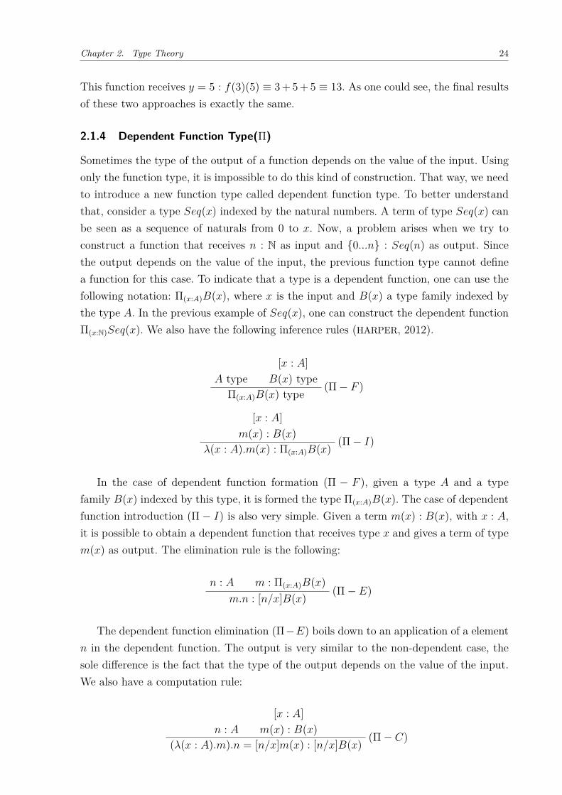
2.1.4 Dependent Function Type(Π)
Sometimes the type of the output of a function depends on the value of the input. Usingonly the function type, it is impossible to do this kind of construction. That way, we needto introduce a new function type called dependent function type. To better understandthat, consider a type 𝑆𝑒𝑞(𝑥) indexed by the natural numbers. A term of type 𝑆𝑒𝑞(𝑥) canbe seen as a sequence of naturals from 0 to 𝑥. Now, a problem arises when we try toconstruct a function that receives 𝑛 : N as input and {0...𝑛} : 𝑆𝑒𝑞(𝑛) as output. Sincethe output depends on the value of the input, the previous function type cannot definea function for this case. To indicate that a type is a dependent function, one can use thefollowing notation: Π(𝑥:𝐴)𝐵(𝑥), where 𝑥 is the input and 𝐵(𝑥) a type family indexed bythe type 𝐴. In the previous example of 𝑆𝑒𝑞(𝑥), one can construct the dependent functionΠ(𝑥:N)𝑆𝑒𝑞(𝑥). We also have the following inference rules (HARPER, 2012).
𝐴 type[𝑥 : 𝐴]
𝐵(𝑥) type (Π − 𝐹 )Π(𝑥:𝐴)𝐵(𝑥) type
[𝑥 : 𝐴]𝑚(𝑥) : 𝐵(𝑥) (Π − 𝐼)
𝜆(𝑥 : 𝐴).𝑚(𝑥) : Π(𝑥:𝐴)𝐵(𝑥)
In the case of dependent function formation (Π − 𝐹 ), given a type 𝐴 and a typefamily 𝐵(𝑥) indexed by this type, it is formed the type Π(𝑥:𝐴)𝐵(𝑥). The case of dependentfunction introduction (Π − 𝐼) is also very simple. Given a term 𝑚(𝑥) : 𝐵(𝑥), with 𝑥 : 𝐴,it is possible to obtain a dependent function that receives type 𝑥 and gives a term of type𝑚(𝑥) as output. The elimination rule is the following:
𝑛 : 𝐴 𝑚 : Π(𝑥:𝐴)𝐵(𝑥)(Π − 𝐸)
𝑚.𝑛 : [𝑛/𝑥]𝐵(𝑥)
The dependent function elimination (Π−𝐸) boils down to an application of a element𝑛 in the dependent function. The output is very similar to the non-dependent case, thesole difference is the fact that the type of the output depends on the value of the input.We also have a computation rule:
𝑛 : 𝐴[𝑥 : 𝐴]
𝑚(𝑥) : 𝐵(𝑥) (Π − 𝐶)(𝜆(𝑥 : 𝐴).𝑚).𝑛 = [𝑛/𝑥]𝑚(𝑥) : [𝑛/𝑥]𝐵(𝑥)

Chapter 2. Type Theory 25
If one looks closely, the dependent function computation (Π −𝐶) establishes functionapplication the exactly way that was defined in non-dependent functions. The sole dif-ference is that the output depends on 𝑥. With that, we have all necessary rules to defineand compute dependent functions. Also, when working directly with types that representpropositions, one should can semantically interpret a type Π(𝑥:𝐴)𝐵(𝑥) as ∀(𝑥 : 𝐴)𝐵(𝑥).
2.1.5 Product type (×)
Previously we have mentioned the existence of multivariable functions, that receives twoor more inputs. But how can we represent a function that, for instance, receives twonatural numbers? In set theory, one could use the cross product to do that. That way,this function receives N×N as input. In this sense, it is essential to define cross productin the framework of type theory.
Intuitively, for any types 𝐴 and 𝐵 one should be able to construct the type 𝐴 × 𝐵.A term of 𝐴 × 𝐵 is a pair (𝑎, 𝑏) : 𝐴 × 𝐵, with 𝑎 : 𝐴 and 𝑏 : 𝐵. This is formalized in thefollowing rules (QUEIROZ; OLIVEIRA; GABBAY, 2011):
𝐴 type 𝐵 type (× − 𝐹 )𝐴×𝐵 type
𝑎 : 𝐴 𝑏 : 𝐵 (× − 𝐼)(𝑎, 𝑏) : 𝐴×𝐵
If one looks closely, if 𝐴 and 𝐵 are propositions, 𝐴× 𝐵 can be interpreted as 𝐴 ∧ 𝐵.That way, one should be able to infer 𝐴 and 𝐵 from 𝐴 × 𝐵. To do that, we introducefunctions 𝐹𝑆𝑇 and 𝑆𝑁𝐷 (QUEIROZ; OLIVEIRA; GABBAY, 2011):
⟨𝑎, 𝑏⟩ : 𝐴×𝐵 (× − 𝐸1)𝐹𝑆𝑇 ((𝑎, 𝑏)) : 𝐴
(𝑎, 𝑏) : 𝐴×𝐵 (× − 𝐸2)𝑆𝑁𝐷((𝑎, 𝑏)) : 𝐵
Using 𝐹𝑆𝑇 and 𝑆𝑁𝐷 functions, we want to be able to retrieve the first and sec-ond elements of a pair ⟨𝑎, 𝑏⟩ respectively. Thus, we have the following computation rules(QUEIROZ; OLIVEIRA; GABBAY, 2011):
(𝑎, 𝑏) : 𝐴×𝐵 × − 𝐸1 B𝛽 𝑎 : 𝐴𝐹𝑆𝑇 ((𝑎, 𝑏)) : 𝐴
(𝑎, 𝑏) : 𝐴×𝐵 × − 𝐸2 B𝛽 𝑏 : 𝐴𝑆𝑁𝐷((𝑎, 𝑏)) : 𝐵
The above rules are called ×-reductions. We also have another computation rule called×-induction (QUEIROZ; OLIVEIRA; GABBAY, 2011):

Chapter 2. Type Theory 26
𝑐 : 𝐴×𝐵 × − 𝐸1𝐹𝑆𝑇 (𝑐) : 𝐴
𝑐 : 𝐴×𝐵 × − 𝐸2𝑆𝑁𝐷(𝑐) : 𝐵 × − 𝐼 B𝜂 𝑐 : 𝐴×𝐵
(𝐹𝑆𝑇 (𝑐), 𝑆𝑁𝐷(𝑐)) : 𝐴×𝐵
2.1.6 Coproduct (+)
In the previous subsection we have introduced the product type. We saw that × can beseen semantically as a cross product in set theory and the connector ∧ when dealing withpropositions. Thus, it is natural to think that the dual of the product should also be ableto be formalized in type theory. That is what we do in this section. In set theory, thecoproduct represents the disjoint union. If one is working with propositions, the coproductcan be semantically interpreted as the connector ∨.
In the product, we have seen that from a term of 𝐴×𝐵 one should be able to obtainterms of 𝐴 and 𝐵 by separate processes. Since the coproduct work as the dual of theproduct, then it is natural to think that one should be able to obtain a term of 𝐴 + 𝐵
from a term of 𝐴 or a term of 𝐵. That is exactly what happens (QUEIROZ; OLIVEIRA;
GABBAY, 2011):
𝐴 type 𝐵 type (+ − 𝐹 )𝐴+𝐵 type
𝑎 : 𝐴 (+ − 𝐼1)𝑖𝑛𝑙(𝑎) : 𝐴+𝐵
𝑏 : 𝐵 (+ − 𝐼2)𝑖𝑛𝑟(𝑏) : 𝐴+𝐵
The elimination rule follows directly from the fact that if one from 𝑎 : 𝐴 is able toconstruct a term 𝑟(𝑎) : 𝐶 and from 𝑏 : 𝐵 we also construct 𝑙(𝑏) : 𝐶, then we should beable to construct one term of type 𝐶 directly from a term 𝑐 : 𝐴+𝐵 (QUEIROZ; OLIVEIRA;
GABBAY, 2011):
𝑐 : 𝐴+𝐵
[𝑎 : 𝐴]𝑟(𝑎) : 𝐶
[𝑏 : 𝐵]𝑙(𝑏) : 𝐶 (+ − 𝐸)
𝐶𝐴𝑆𝐸(𝑐, �́�𝑟(𝑎), �́�𝑙(𝑏)) : 𝐶
One should see 𝑑(𝑎) and 𝑒(𝑏) as functional expressions dependent on 𝑎 and 𝑏 respec-tively. One should also notice the use of ‘́ ’ in �́� and �́�. One should see ‘́ ’ as an abstractorthat binds the occurrences of the variable 𝑎 and 𝑏 both introduced in the local assump-tions. We have the following reduction rules (QUEIROZ; OLIVEIRA; GABBAY, 2011):
𝑐 : 𝐴𝑖𝑛𝑙(𝑐) : 𝐴+𝐵
[𝑎 : 𝐴]𝑟(𝑎) : 𝐶
[𝑏 : 𝐵]𝑙(𝑏) : 𝐶 (+ − 𝐸) B𝛽
𝐶𝐴𝑆𝐸(𝑖𝑛𝑙(𝑐), �́�𝑟(𝑎), �́�𝑙(𝑏)) : 𝐶
[𝑐 : 𝐴][𝑐/𝑥]𝑟(𝑎) : 𝐶

Chapter 2. Type Theory 27
𝑐 : 𝐵𝑖𝑛𝑟(𝑐) : 𝐴+𝐵
[𝑎 : 𝐴]𝑟(𝑎) : 𝐶
[𝑏 : 𝐵]𝑙(𝑏) : 𝐶 (+ − 𝐸) B𝛽
𝐶𝐴𝑆𝐸(𝑖𝑛𝑟(𝑐), �́�𝑟(𝑎), �́�𝑙(𝑏)) : 𝐶
[𝑐 : 𝐵][𝑐/𝑥]𝑙(𝑏) : 𝐶
We also have an induction rule (QUEIROZ; OLIVEIRA; GABBAY, 2011):
𝑐 : 𝐴+𝐵
[𝑎 : 𝐴] + − 𝐼1𝑖𝑛𝑙(𝑎) : 𝐴+𝐵
[𝑏 : 𝐵] + − 𝐼2𝑖𝑛𝑟(𝑦) : 𝐴+𝐵 + − 𝐸 B𝜂
𝐶𝐴𝑆𝐸(𝑐, ´(𝑎)𝑖𝑛𝑙(𝑎), �́�𝑖𝑛𝑟(𝑏)) : 𝐴+𝐵𝑐 : 𝐴+𝐵
2.1.7 Dependent Pair Type (Σ)
When working with functions, it is sometimes useful to work with ordered pairs (𝑎, 𝑏)such that 𝑎 is a input for the function and 𝑏 is the respective output. But what happensif one is working with a dependent function? In that case, the type of the output 𝑏would be bounded to the value of the input 𝑎. To represent this, one needs to use a typecalled dependent pair. The notation for this type is Σ(𝑥:𝐴)𝐵(𝑥) and it has the followingrules(HARPER, 2012):
𝐴 type[𝑥 : 𝐴]
𝐵(𝑥) type (Σ − 𝐹 )Σ(𝑥:𝐴)𝐵(𝑥) type
𝑚 : 𝐴 𝑛 : 𝐵(𝑚) (Σ − 𝐼)⟨𝑚,𝑛⟩ : Σ(𝑥:𝐴)𝐵(𝑥)
The dependent sum formation (Σ − 𝐹 ) is similar to Π − 𝐹 . For dependent sum intro-duction (Σ − 𝐼), an element 𝑚 : 𝐴 and an element 𝑛 : 𝐵(𝑚) are enough to introduce adependent pair ⟨𝑚,𝑛⟩ : Σ(𝑥:𝐴)𝐵(𝑥). We have two elimination rules:
𝑚 : Σ(𝑥:𝐴)𝐵(𝑥)(Σ − 𝐸1)
𝜋1(𝑚) : 𝐴
𝑚 : Σ(𝑥:𝐴)𝐵(𝑥)(Σ − 𝐸2)
𝜋2(𝑚) : [𝜋1(𝑚)/𝑥]𝐵(𝑥)
In traditional type theory, the dependent pair has two eliminations. This is explainedby the fact that since the pair is composed by two terms, it is possible to eliminateΣ obtaining the first or the second term. From a dependent pair, one can use the firstdependent sum elimination (Σ − 𝐸1) and extract the first element. From the seconddependent sum elimination (Σ − 𝐸2) one can extract the second element, which typedepends on the value of the first element. Thus, we have two computation rules:

Chapter 2. Type Theory 28
𝜋1(⟨𝑚,𝑛⟩) = 𝑚 e 𝜋2(⟨𝑚,𝑛⟩) = 𝑛.
The operators 𝜋1 and 𝜋2 extract the necessary information from the dependent pair.One obtains 𝑚 and 𝑛 respectively. The dependent pair should be understood as the dualof the dependent product.
2.1.8 Alternative Formulation for the Dependent Pair
If one is working within the paradigm of formulae-as-types(HOWARD, 1980), the depen-dent product should be semantically interpreted as the ∃ quantifier. Nevertheless, it hasbeen pointed out by(QUEIROZ; GABBAY, 1995) that the previous formulation for the de-pendent pair leads to problems. The main issue is the fact that the previous formulationdoes not ’hide’ the witness in an existential formula. One can apply directly 𝜋1 to adependent pair, obtaining the witness and ignoring the fact that it should be hidden.Thus,(QUEIROZ; GABBAY, 1995) argues that this ’availability’ does not match with thetrue spirit of indefiniteness of the existential qualifier. To better see this, one could con-sider the fact that the duality between the existential and universal quantifiers are thefirst-order counterpart of the duality between the disjunction and the conjunction. In thelanguage of type theory, when one talks about conjunction one is really talking about×-product. In the ×-product, the terms of a pair are readily available:
𝑎 : 𝐴 𝑏 : 𝐵 × − 𝐼(𝑎, 𝑏) : 𝐴×𝐵× − 𝐸1
𝐹𝑆𝑇 ((𝑎, 𝑏)) : 𝐴
𝑎 : 𝐴 𝑏 : 𝐵 × − 𝐼(𝑎, 𝑏) : 𝐴×𝐵× − 𝐸2
𝑆𝑁𝐷((𝑎, 𝑏)) : 𝐵
In the case of the disjunction, i.e., the coproduct in type theory, once one of thedisjuncts is used to construct a term of the coproduct, it becomes ’hidden’, the elimina-tion rule has to proceed by Skolem-like introductions of new local assumptions(QUEIROZ;
GABBAY, 1995):
𝑎 : 𝐴 + − 𝐼𝑖𝑛𝑙(𝑎) : 𝐴+𝐵
[𝑥 : 𝐴]𝑟(𝑥) : 𝐶
[𝑦 : 𝐵]𝑙(𝑦) : 𝐶 + − 𝐸1
𝐶𝐴𝑆𝐸(𝑖𝑛𝑙(𝑎), �́�𝑟(𝑥), 𝑦𝑙(𝑦))
𝑏 : 𝐵 + − 𝐼𝑖𝑛𝑟(𝑏) : 𝐴+𝐵
[𝑥 : 𝐴]𝑟(𝑥) : 𝐶
[𝑦 : 𝐵]𝑙(𝑦) : 𝐶 + − 𝐸2
𝐶𝐴𝑆𝐸(𝑖𝑛𝑟(𝑏), �́�𝑟(𝑥), 𝑦𝑙(𝑦))
In the first case, one has 𝑎 : 𝐴 in the start, but after introducing 𝑖𝑛𝑙(𝑎) : 𝐴 + 𝐵, 𝑎becomes hidden, i.e., one loses direct access to it. The same thing happens to 𝑏 : 𝐵 and𝑖𝑛𝑟(𝑏) : 𝐴 + 𝐵 in the second case. Thus, one proceeds adding local assumptions 𝑥 : 𝐴and 𝑦 : 𝐵. With that in mind, (QUEIROZ; GABBAY, 1995) showed that the existential

Chapter 2. Type Theory 29
should mirror this aspect. The witness should be hidden and one should proceed byintroducing Skolem-like local assumptions. Thus, the elimination rule for the dependentpair is reformulated (QUEIROZ; GABBAY, 1995):
𝑛 : Σ(𝑥:𝐴)𝐵(𝑥)[𝑡 : 𝐴, 𝑓(𝑡) : 𝐵(𝑡)]
ℎ(𝑡, 𝑓) : 𝐶(Σ − 𝐸)
𝐸(𝑛, 𝑡𝑓ℎ(𝑡, 𝑓)) : 𝐶
This elimination rule eliminates the dependent pair without giving direct access tothe witness. Of course, it generates new computation rules. Here follows the reductionrule(QUEIROZ; GABBAY, 1995):
𝑎 : 𝐷 𝑓(𝑎) : 𝐹 (𝑎)Σ − 𝐼⟨𝑎, 𝑓(𝑎)⟩ : Σ(𝑥:𝐷)𝐹 (𝑥)
𝑡 : 𝐷, 𝑔(𝑡) : 𝐹 (𝑡)𝑑(𝑔, 𝑡) : 𝐶
Σ − 𝐸 B𝛽𝐸(⟨𝑎, 𝑓(𝑎)⟩ , 𝑔𝑡𝑑(𝑔, 𝑡)) : 𝐶
[𝐴 : 𝐷, 𝑓(𝑎) : 𝐹 (𝑎)][𝑓/𝑔, 𝑎/𝑡]𝑑(𝑔, 𝑡)
The last rule is the induction(QUEIROZ; GABBAY, 1995):
𝑐 : Σ(𝑥:𝐷)𝑃 (𝑥)[𝑡 : 𝐷] [𝑔(𝑡) : 𝑃 (𝑡)]
Σ − 𝐼⟨𝑡, 𝑔(𝑡)⟩ : Σ(𝑦:𝐷)𝑃 (𝑦)Σ − 𝐸 B𝜂 𝑐 : Σ(𝑥:𝐷)𝑃 (𝑥)
𝐸(𝑐, 𝑔𝑡 ⟨𝑡, 𝑔(𝑡)⟩) : Σ(𝑦:𝐷)𝑃 (𝑦)
2.1.9 The Natural Numbers
It has been said that one of the main objectives that motivated type theory was thefact that it worked as a foundation for constructive mathematics. Thus, a theory thatproposes to be a foundation for mathematics should at least be able to formalize thenatural numbers. Set theory, for example, is capable of doing that. Thus, the objective ofthis subsection is to show how the natural numbers can be constructed in type theory andto show some basic properties of the naturals. As always, we start with basic constructions:(HARPER, 2012):
(N− 𝐼0)0 : N𝑚 : N (N− 𝐼𝑠)
𝑠𝑢𝑐𝑐(𝑚) : N

Chapter 2. Type Theory 30
The natural are constructed in a simple way, from the two rules above. The zerointroduction (N− 𝐼0) should be understood as the base of the construction. It states theexistence of at least one term called 0 that is a term of N. From a term 𝑚 : N, one canapply the successor induction (N−𝐼𝑠) to obtain another term of type 𝑠𝑢𝑐𝑐(𝑚) : N. Thus, ifone starts from 0 and inductively construct numbers applying 𝑠𝑢𝑐𝑐, one wind up with theentire set of natural numbers. Nevertheless, those two rules does not give us the tools towork with the natural numbers. Ideally, one wants to construct functions on the naturalsand also apply the inductive principle to construct proofs. Those tools are given by thecomputation rules. Let’s start with the non-dependent case (HARPER, 2012):
𝑚 : N 𝐶 type 𝑁0 : 𝐶[𝑥 : 𝐶]𝑁𝑠 : 𝐶
𝑟𝑒𝑐(𝑚,𝑁0, 𝜆𝑥.𝑁𝑠) : 𝐶
The inference rule above can be rather confusing. The idea is to use a recursor 𝑟𝑒𝑐 todefine basic functions on the naturals, such as addition, multiplication and exponentiation.The recursor receives a base case 𝑁0, that states how 𝑟𝑒𝑐 should act when it iterates 0times. Another piece of information is that given 𝑥 iterations, the recursor needs to knowhow to compute the next iteration. This next iteration is represented by 𝑁𝑠. Thus, basedon the inductive definition of the naturals, this is enough to define how any function on thenaturals works. To better illustrate that, let’s use 𝑟𝑒𝑐 to define addition. Given 𝑚,𝑛 : N,we want 𝑚+𝑛 : N. Starting from 𝑚, one can define the base case to be 𝑚+0 = 𝑚. Thus,one just needs to iterate 𝑛 times the function 𝑠𝑢𝑐𝑐 starting from 𝑚. This is expressed asfollowing:
𝑚 : N N type 𝑚 : N[𝑛 : N]
𝑠𝑢𝑐𝑐(𝑛) : N𝑟𝑒𝑐(𝑚,𝑚, 𝜆𝑛.𝑠𝑢𝑐𝑐(𝑛)) : N
𝜆𝑚.𝑟𝑒𝑐(𝑚,𝑚, 𝜆𝑛.𝑠𝑢𝑐𝑐(𝑛)) : N → N
This rule used to define recursive functions on the naturals is called the non-dependentcase, since it originates terms of a non-dependent type 𝐶. To use the induction principle,one needs to define the dependent case (HARPER, 2012):
𝑚 : N[𝑥 : N]
𝐶(𝑥) type 𝑁0 : [0/𝑥]𝐶(𝑥)[𝑥 : N, 𝑦 : 𝐶(𝑥)]
𝑁𝑠 : [𝑠𝑢𝑐(𝑥)/𝑥]𝐶(𝑥)𝑟𝑒𝑐(𝑚,𝑁0, (𝑥, 𝜆𝑦.𝑁𝑠)) : [𝑚/𝑥]𝐶(𝑥)
If one looks closely, one should notice that the non-dependent case is the inductionprinciple of the natural numbers. Basically, it states that given a proof of the base case

Chapter 2. Type Theory 31
𝑁0 : 𝐶(0) and the inductive step, i.e., that a proof 𝑦 : 𝐶(𝑥) implies a proof of 𝑁𝑠 : 𝐶(𝑥+1),then one should wind up with a proof 𝐶(𝑚) for any 𝑚 : N. With that, we conclude theconstruction and main properties used to work with the naturals in type theory.
2.1.10 Additional Information
We have said that a type can be semantically interpreted in different ways. It can be aproposition, a topological space, a set, among others semantical interpretation. The mainones are summed up in the table below:
Table 1 – Multiple semantical interpretations of a type
Types Logic Sets Homotopy𝐴 proposition set space𝑎 : 𝐴 proof element point𝐵(𝑥) predicate family of sets fibration𝑏(𝑥) : 𝐵(𝑥) conditional proof family of elements section0,1 ⊥,⊤ ∅, {∅} ∅, *𝐴 + 𝐵 𝐴 ∨ 𝐵 disjoint union coproduct𝐴 × 𝐵 𝐴 ∧ 𝐵 set of pairs product space𝐴 → 𝐵 𝐴 ⇒ 𝐵 set of functions function spaceΣ𝑥:𝐴𝐵(𝑥) ∃(𝑥:𝐴)𝐵(𝑥) disjoint sum total spaceΠ𝑥:𝐴𝐵(𝑥) ∀(𝑥:𝐴)𝐵(𝑥) product space of sections𝐼𝑑𝑎 equality = {(𝑥, 𝑥) | 𝑥 ∈ 𝐴} path space 𝐴𝐼
Source: Homotopy Type Theory Book (Univalent Foundations Program, 2013).
As one can see, type theory is capable of representing many diverse objects of mathe-matics and logic. In the previous subsections, we have shown the basic constructions thateveryone interested in type theory should be familiar with. Nevertheless, we have nottalked about the identity type yet. Since it is a type of central to the main contributionof this work, the next section is completely focused on explaining it.
2.2 IDENTITY TYPE
After briefly introducing the main concepts and types of type theory, the objective of thissection is to introduce the main entity of this work, the identity type. Here we are goingto introduce the classic approach of type theory. One can check our proposed formulationfor the identity type in chapter 4 of this work.
The identity type is arguably the most interesting concept of type theory. This claimis based on the fact that many results have been achieved using it. One of these wasthe discovery of the Univalent Models in 2005 by Vladimir Voevodsky (VOEVODSKY,2014). From this work, a groundbreaking result has arisen: the connection between type

Chapter 2. Type Theory 32
theory and homotopy theory. The intuitive connection is simple: a term 𝑎 : 𝐴 can beconsidered as a point of the space 𝐴 and 𝑝 : 𝐼𝑑𝐴(𝑎, 𝑏) is a homotopy path between points𝑎, 𝑏 ∈ 𝐴(Univalent Foundations Program, 2013). This has given rise to a whole new area ofresearch, known as Homotopy Type Theory. It leads to a new perspective on the study ofequality, as expressed by Voevodsky in a recent talk in The Paul Bernays Lectures (Sept2014, Zürich): equality (for abstract sets) should be looked at as a structure rather thanas a relation.
2.2.1 Formal Definition of The Identity Type
We start with the formation and introduction rules (QUEIROZ; OLIVEIRA, 2014b):
𝐴 type 𝑎 : 𝐴 𝑏 : 𝐴𝐼𝑑𝑖𝑛𝑡 − 𝐹
𝐼𝑑𝑖𝑛𝑡𝐴 (𝑎, 𝑏) type
𝑎 : 𝐴𝐼𝑑𝑖𝑛𝑡 − 𝐼
𝑟(𝑎) : 𝐼𝑑𝑖𝑛𝑡𝐴 (𝑎, 𝑎)
First, we need to clarify the meaning of 𝑖𝑛𝑡 that appears in 𝐼𝑑𝑖𝑛𝑡. This 𝑖𝑛𝑡 indicatesthat we are working with the intensional version of the identity type. The differencebetween the intensional and extensional version will be explained in detail in the nextsubsection. For now, let’s postulate that every time 𝑖𝑛𝑡 or 𝑒𝑥𝑡 do not appear above 𝐼𝑑𝐴,one should assume that the version being used is the intensional one.
The identity type formation (𝐼𝑑𝑖𝑛𝑡 − 𝐹 ) is pretty straightforward. Given any terms𝑎, 𝑏 : 𝐴, it is possible to create a type that will only be inhabited if there exits an witnessthat testifies the propositional equality between 𝑎 and 𝑏. Nevertheless, the existence oftype 𝐼𝑑𝐴(𝑎, 𝑏) does not dependent on whether it is inhabited or not.
The rule identity type introduction (𝐼𝑑𝑖𝑛𝑡 − 𝐼) states that there is only one canonicalproof of equality, the reflexivity. It states that any term 𝑎 : 𝐴 is always propositionalequal to itself. This introduces a canonical proof of reflexivity 𝑟(𝑎) : 𝐼𝑑𝑖𝑛𝑡
𝐴 (𝑎, 𝑎). Thus, themain idea is that every proof of equality can be constructed inductively from a reflexiveproof of equality (QUEIROZ; OLIVEIRA, 2014b):
𝑎 : 𝐴 𝑏 : 𝐴 𝑐 : 𝐼𝑑𝑖𝑛𝑡𝐴 (𝑎, 𝑏)
[𝑥 : 𝐴]𝑑(𝑥) : 𝐶(𝑥, 𝑥, 𝑟(𝑥))
[𝑥 : 𝐴, 𝑦 : 𝐴, 𝑧 : 𝐼𝑑𝐴(𝑥, 𝑦)]𝐶(𝑥, 𝑦, 𝑧) type
𝐼𝑑− 𝐸𝐽(𝑐, 𝑑) : 𝐶(𝑎, 𝑏, 𝑐)
𝑎 : 𝐴[𝑥 : 𝐴]
𝑑(𝑥) : 𝐶(𝑥, 𝑥, 𝑟(𝑥))[𝑥 : 𝐴, 𝑦 : 𝐴, 𝑧 : 𝐼𝑑𝐴(𝑥, 𝑦)]
𝐶(𝑥, 𝑦, 𝑧) type𝐼𝑑− 𝐸𝑞
𝐽(𝑟(𝑎), 𝑑(𝑥)) = 𝑑(𝑎/𝑥) : 𝐶(𝑎, 𝑎, 𝑟(𝑎))

Chapter 2. Type Theory 33
The identity type elimination (𝐼𝑑 − 𝐸) introduces the recursor 𝐽 and eliminates theidentity type in the process. The inner details of the recursor 𝐽 are pretty complicatedto understand and uses complex concepts of category theory. Nevertheless, one can tryto intuitively understand 𝐽 . Basically, 𝐽(𝑐, 𝑑) : 𝐶(𝑎, 𝑏, 𝑐) works constructing 𝑐 from areflexive proof 𝑑. In this case, as any recursor of type theory, 𝑐 is constructed based onmultiple iterations that starts from the base 𝑑. Since this elimination rule has many terms,constructing some types using 𝐽 can be a cumbersome process, as we are going to seein the next subsection. In this work, we are going to introduce a way of formalizing theidentity type using a new entity known as computational paths. We believe that this wayis simpler and more straightforward to use than the one introduced here. Nevertheless,we leave this discussion to a further chapter of this work.
2.2.2 Basic Constructions
The objective of this subsection is to show the use of the elimination rule of the identitytype in practice. The constructions that we have chosen to build are the reflexive, transitiveand symmetric type of the identity type. Those were not random choices. The main reasonis the fact that reflexive, transitive and symmetric types are essential to the process ofbuilding a groupoid model for the identity type (HOFMANN; STREICHER, 1994).
Before we start the constructions, we think that it is essential to understand how to usethe eliminations rules. The process of building a term of some type is a matter of findingthe right reason. In the case of 𝐽 , the reason is the correct 𝑥, 𝑦 : 𝐴 and 𝑧 : 𝐼𝑑𝐴(𝑎, 𝑏) thatgenerates the adequate 𝐶(𝑥, 𝑦, 𝑧).
We start proving the reflexivity. We want a witness for Π(𝑎:𝐴)𝐼𝑑𝐴(𝑎, 𝑎). This case istrivial, since we have the canonical proof of identity:
𝑎 : 𝐴 𝐼𝑑− 𝐼𝑟(𝑎) : 𝐼𝑑𝐴(𝑎, 𝑎)
The second construction is the symmetry. This one does not follow trivially from theintroduction rule. Thus, we need to use the elimination rule in some way. Our objectiveis to construct a term for the type Π(𝑎:𝐴)Π(𝑏:𝐴)(𝐼𝑑𝐴(𝑎, 𝑏) → 𝐼𝑑𝐴(𝑏, 𝑎)).
Looking at the elimination rule of the constructor J, it is clear that our main objectiveis to find a suitable 𝐶(𝑥, 𝑦, 𝑧), with 𝑥 : 𝐴, 𝑦 : 𝐴 and 𝑧 : 𝐼𝑑𝐴(𝑎, 𝑏). The main problem isthe fact that, to find the correct reason, we do not have a fixed process or a fixed set ofrules to follow. One needs to rely on one’s intuition. In this case, one could conclude thatthe correct reason is to look at 𝐶(𝑥, 𝑦, , 𝑧) as the type 𝐼𝑑𝐴(𝑦, 𝑥), with 𝑥 : 𝐴, 𝑦 : 𝐴 and 𝑧
as any term (in the deduction, 𝑧 will be represented by −, to indicate that it can be anyterm). Thus, we obtain the following deduction:

Chapter 2. Type Theory 34
𝑎 : 𝐴 𝑏 : 𝐴 𝑐 : 𝐼𝑑𝐴(𝑎, 𝑏)[𝑥 : 𝐴]
𝑟(𝑥) : 𝐼𝑑𝐴(𝑥, 𝑥)[𝑥 : 𝐴, 𝑦 : 𝐴,− : 𝐼𝑑𝐴(𝑎, 𝑏)]
𝐼𝑑𝐴(𝑦, 𝑥) type𝐼𝑑− 𝐸
𝐽(𝑐, 𝑟(𝑥)) : 𝐼𝑑𝐴(𝑏, 𝑎)→ −𝐼
𝜆𝑐.𝐽(𝑐, 𝑟(𝑥)) : 𝐼𝑑𝐴(𝑎, 𝑏) → 𝐼𝑑𝐴(𝑏, 𝑎)Π − 𝐼
𝜆𝑏.𝜆𝑐.𝐽(𝑐, 𝑟(𝑥)) : Π(𝑏:𝐴)(𝐼𝑑𝐴(𝑎, 𝑏) → 𝐼𝑑𝐴(𝑏, 𝑎))Π − 𝐼
𝜆𝑎.𝜆𝑏.𝜆𝑐.𝐽(𝑐, 𝑟(𝑥)) : Π(𝑎:𝐴)Π(𝑏:𝐴)(𝐼𝑑𝐴(𝑎, 𝑏) → 𝐼𝑑𝐴(𝑏, 𝑎))
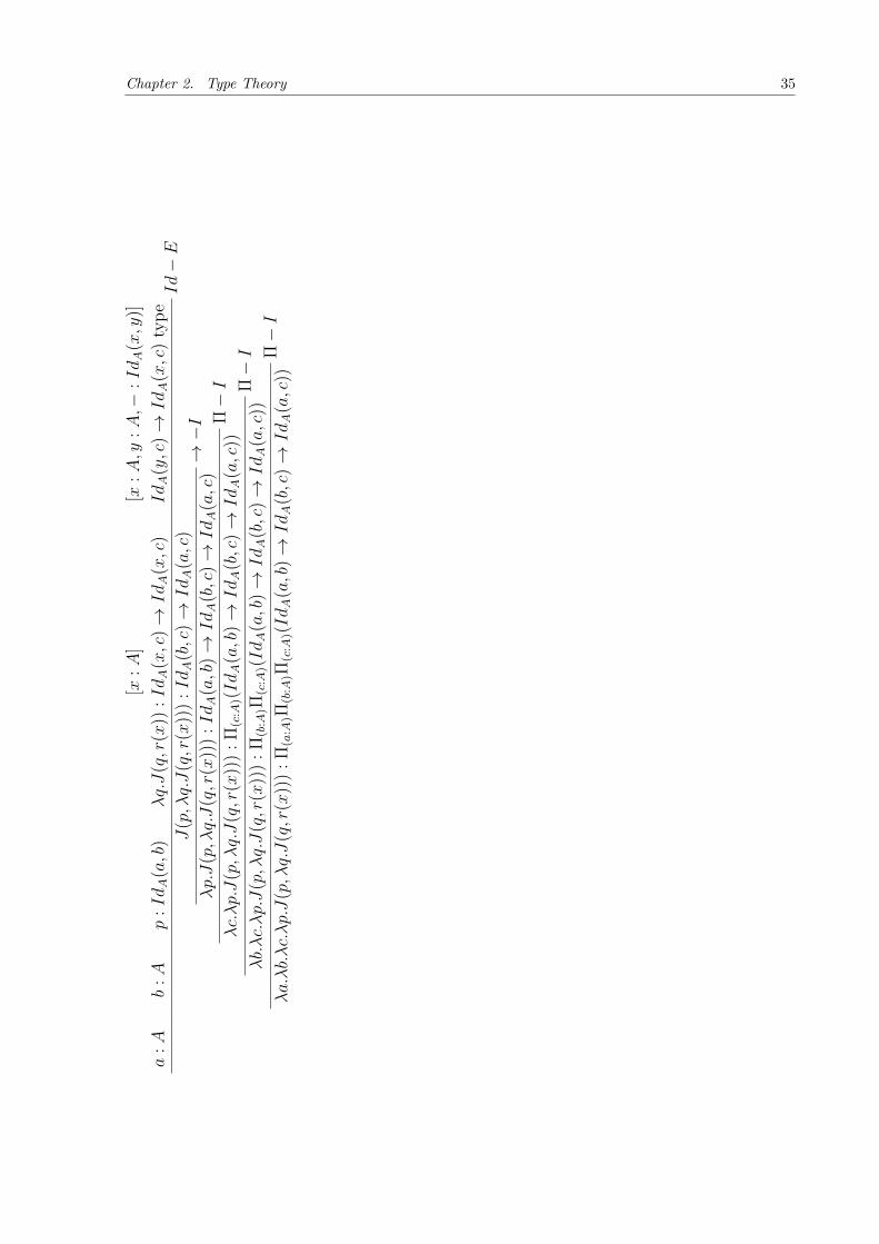
The third and last construction will be the transitivity. Our objective is to constructa term for the type Π(𝑎:𝐴)Π(𝑏:𝐴)Π(𝑐:𝐴)(𝐼𝑑𝐴(𝑎, 𝑏) → 𝐼𝑑𝐴(𝑏, 𝑐) → 𝐼𝑑𝐴(𝑎, 𝑐)).
Let’s now use 𝐽 to build a term for the transitivity. The proof will be based on theone found in (Univalent Foundations Program, 2013). The difference is that instead of defininginduction principles for 𝐽 based on the elimination rules, we will use the rule directly.The complexity is the same, since the proofs are two forms of presenting the same thingand they share the same reasons. As one should expect, the first and main step is tofind a suitable reason. In other words, we need to find suitable 𝑥, 𝑦 : 𝐴 and 𝑧 : 𝐼𝑑𝐴(𝑎, 𝑏)to construct an adequate 𝐶(𝑥, 𝑦, 𝑧). Similar to the case of symmetry, this first step isalready problematic. Different from our approach, in which one starts from a path andapplies intuitive equality axioms to find a suitable reason, there is no clear point of howone should proceed to find a suitable reason for the construction based on 𝐽 . In thiscase, one should rely on intuition and make attempts until one finds out the correctreason. As one can check in (Univalent Foundations Program, 2013), a suitable reason wouldbe 𝑥 : 𝐴, 𝑦 : 𝐴,− : 𝐼𝑑𝐴(𝑥, 𝑦) and 𝐶(𝑥, 𝑦, 𝑧) ≡ 𝐼𝑑𝐴(𝑦, 𝑐) → 𝐼𝑑𝐴(𝑥, 𝑐). Looking closely,the proof is not over yet. The problem is the type of 𝐶(𝑥, 𝑥, 𝑟(𝑥)). With this reason,we have that 𝐶(𝑥, 𝑥, 𝑟(𝑥)) ≡ 𝐼𝑑𝐴(𝑥, 𝑐) → 𝐼𝑑𝐴(𝑥, 𝑐). Therefore, we cannot assume that𝑞(𝑥) : 𝐼𝑑𝐴(𝑥, 𝑐) → 𝐼𝑑𝐴(𝑥, 𝑐) is the term 𝑟(𝑥). The only way to proceed is to apply againthe constructor 𝐽 to build the term 𝑞(𝑥). It means, of course, that we will need to find yetanother reason to build this type. This second reason is given by 𝑥 : 𝐴, 𝑦 : 𝐴,− : 𝐼𝑑𝐴(𝑥, 𝑦)and 𝐶 ′(𝑥, 𝑦, 𝑧) ≡ 𝐼𝑑𝐴(𝑥, 𝑦). In that case, 𝐶 ′(𝑥, 𝑥, 𝑟(𝑥)) = 𝐼𝑑𝐴(𝑥, 𝑥). We will not need touse 𝐽 again, since now we have that 𝑟(𝑥) : 𝐼𝑑𝐴(𝑥, 𝑥). Then, we can construct 𝑞(𝑥):
𝑥 : 𝐴 𝑐 : 𝐴 𝑞 : 𝐼𝑑𝐴(𝑥, 𝑐)[𝑥 : 𝐴]
𝑟(𝑥) : 𝐼𝑑𝐴(𝑥, 𝑥)[𝑥 : 𝐴, 𝑦 : 𝐴,− : 𝐼𝑑𝐴(𝑥, 𝑦)]
𝐼𝑑𝐴(𝑥, 𝑦) type𝐼𝑑− 𝐸
𝐽(𝑞, 𝑟(𝑥)) : 𝐼𝑑𝐴(𝑥, 𝑐)→ −𝐼
𝜆𝑞.𝐽(𝑞, 𝑟(𝑥)) : 𝐼𝑑𝐴(𝑥, 𝑐) → 𝐼𝑑𝐴(𝑥, 𝑐)
Finally, we obtain the desired term:
Chapter 2. Type Theory 35
𝑎:𝐴
𝑏:𝐴
𝑝:𝐼𝑑
𝐴(𝑎,𝑏
)[𝑥
:𝐴]
𝜆𝑞.𝐽
(𝑞,𝑟
(𝑥))
:𝐼𝑑
𝐴(𝑥,𝑐
)→𝐼𝑑
𝐴(𝑥,𝑐
)[𝑥
:𝐴,𝑦
:𝐴,−
:𝐼𝑑
𝐴(𝑥,𝑦
)]𝐼𝑑
𝐴(𝑦,𝑐
)→𝐼𝑑
𝐴(𝑥,𝑐
)ty
pe𝐼𝑑
−𝐸
𝐽(𝑝,𝜆𝑞.𝐽
(𝑞,𝑟
(𝑥))
):𝐼𝑑
𝐴(𝑏,𝑐
)→𝐼𝑑
𝐴(𝑎,𝑐
)→
−𝐼
𝜆𝑝.𝐽
(𝑝,𝜆𝑞.𝐽
(𝑞,𝑟
(𝑥))
):𝐼𝑑
𝐴(𝑎,𝑏
)→𝐼𝑑
𝐴(𝑏,𝑐
)→𝐼𝑑
𝐴(𝑎,𝑐
)Π
−𝐼
𝜆𝑐.𝜆𝑝.𝐽
(𝑝,𝜆𝑞.𝐽
(𝑞,𝑟
(𝑥))
):Π
(𝑐:𝐴
)(𝐼𝑑
𝐴(𝑎,𝑏
)→𝐼𝑑
𝐴(𝑏,𝑐
)→𝐼𝑑
𝐴(𝑎,𝑐
))Π
−𝐼
𝜆𝑏.𝜆𝑐.𝜆𝑝.𝐽
(𝑝,𝜆𝑞.𝐽
(𝑞,𝑟
(𝑥))
):Π
(𝑏:𝐴
)Π(𝑐
:𝐴)(𝐼𝑑
𝐴(𝑎,𝑏
)→𝐼𝑑
𝐴(𝑏,𝑐
)→𝐼𝑑
𝐴(𝑎,𝑐
))Π
−𝐼
𝜆𝑎.𝜆𝑏.𝜆𝑐.𝜆𝑝.𝐽
(𝑝,𝜆𝑞.𝐽
(𝑞,𝑟
(𝑥))
):Π
(𝑎:𝐴
)Π(𝑏
:𝐴)Π
(𝑐:𝐴
)(𝐼𝑑
𝐴(𝑎,𝑏
)→𝐼𝑑
𝐴(𝑏,𝑐
)→𝐼𝑑
𝐴(𝑎,𝑐
))
Chapter 2. Type Theory 36
This construction is an example that makes clear the difficulties of working withthis approach for the identity type. We had to find two different reasons and use twoapplications of the elimination rule. Another problem is the fact that the reasons werenot obtained by a fixed process, like the applications of axioms in some entity of typetheory. They were obtained purely by the intuition that a certain 𝐶(𝑥, 𝑦, 𝑧) should becapable of constructing the desired term. For that reason, obtaining these reasons can betroublesome.
Further in this work we are going to construct those types using computational paths.Thus, we will have some base on which we can compare the two approaches.
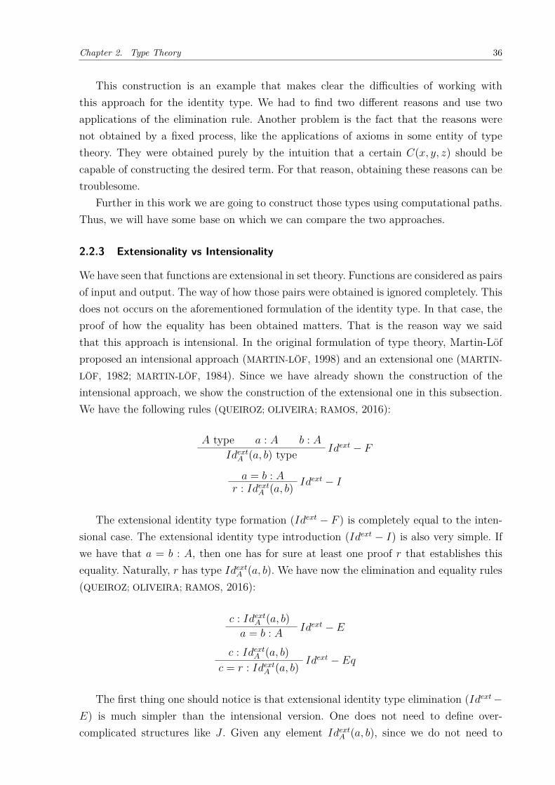
2.2.3 Extensionality vs Intensionality
We have seen that functions are extensional in set theory. Functions are considered as pairsof input and output. The way of how those pairs were obtained is ignored completely. Thisdoes not occurs on the aforementioned formulation of the identity type. In that case, theproof of how the equality has been obtained matters. That is the reason way we saidthat this approach is intensional. In the original formulation of type theory, Martin-Löfproposed an intensional approach (MARTIN-LÖF, 1998) and an extensional one (MARTIN-
LÖF, 1982; MARTIN-LÖF, 1984). Since we have already shown the construction of theintensional approach, we show the construction of the extensional one in this subsection.We have the following rules (QUEIROZ; OLIVEIRA; RAMOS, 2016):
𝐴 type 𝑎 : 𝐴 𝑏 : 𝐴𝐼𝑑𝑒𝑥𝑡 − 𝐹
𝐼𝑑𝑒𝑥𝑡𝐴 (𝑎, 𝑏) type
𝑎 = 𝑏 : 𝐴𝐼𝑑𝑒𝑥𝑡 − 𝐼
𝑟 : 𝐼𝑑𝑒𝑥𝑡𝐴 (𝑎, 𝑏)
The extensional identity type formation (𝐼𝑑𝑒𝑥𝑡 − 𝐹 ) is completely equal to the inten-sional case. The extensional identity type introduction (𝐼𝑑𝑒𝑥𝑡 − 𝐼) is also very simple. Ifwe have that 𝑎 = 𝑏 : 𝐴, then one has for sure at least one proof 𝑟 that establishes thisequality. Naturally, 𝑟 has type 𝐼𝑑𝑒𝑥𝑡
𝐴 (𝑎, 𝑏). We have now the elimination and equality rules(QUEIROZ; OLIVEIRA; RAMOS, 2016):
𝑐 : 𝐼𝑑𝑒𝑥𝑡𝐴 (𝑎, 𝑏)
𝐼𝑑𝑒𝑥𝑡 − 𝐸𝑎 = 𝑏 : 𝐴
𝑐 : 𝐼𝑑𝑒𝑥𝑡𝐴 (𝑎, 𝑏)
𝐼𝑑𝑒𝑥𝑡 − 𝐸𝑞𝑐 = 𝑟 : 𝐼𝑑𝑒𝑥𝑡
𝐴 (𝑎, 𝑏)
The first thing one should notice is that extensional identity type elimination (𝐼𝑑𝑒𝑥𝑡 −𝐸) is much simpler than the intensional version. One does not need to define over-complicated structures like 𝐽 . Given any element 𝐼𝑑𝑒𝑥𝑡
𝐴 (𝑎, 𝑏), since we do not need to

Chapter 2. Type Theory 37
keep track of the equality proof, one can extract directly that 𝑎 = 𝑏 : 𝐶. At this point,the information that 𝑐 is responsible for establishing is irrelevant. As one can see, theexistence of the term 𝑐 is completely excluded of the final inference. The fact that we donot need to keep track of an equality proof is also seen in the extensional identity typeequality (𝐼𝑑𝑒𝑥𝑡 − 𝐸𝑞). This rule shows that any two equality proofs 𝑐 and 𝑟 are equal.Thus, how 𝑐 and 𝑟 are constructed does not matter. The only relevant fact is that theyare both proofs of the equality 𝑎 = 𝑏 : 𝐴.
The approach that we are going to propose based on computational paths will beclearly intensional. This is due to the fact that computation is intrinsically intensional.Two algorithms can solve the same problem, but they can be implemented in completelydifferent ways and have difference space and time complexities. Also, the intensional ver-sion is much more interesting, since it gave rise to homotopy type theory. Thus, this workwill introduce computational paths as an alternative way of formalizing the intensionaltype theory.
2.3 CONCLUSION
In this chapter, we have introduced the basic types of type theory. We showed how toconstruct and compute using those types. We have also highlighted the essential differ-ence between definitional equality and propositional equality. Based on this difference, weshowed how to construct a type based on propositional equality, called identity type.
A good understanding of the basic concepts of this chapter is essential to understandthe main results of this work. In further chapters, we are going to propose a differentway of formalizing intensional identity type. We are going to compare the two approachesusing the basic constructions shown in this chapter. In the next chapter, we are goingto introduce the basic concepts of another theory essential to the results of this work:category theory.

38
3 CATEGORY THEORY
In this chapter, we introduce the theory that we are going to use to develop the math-ematical aspect of computational paths. The theory used to construct this mathematicalmodel will be category theory. We are going to see that this theory is extremely powerful,but it is abstract and complex. With that in mind, we start this chapter defining and ex-posing the main basic concepts of this theory. We then use those basic concepts to arriveat more complicated results, which will be necessary in the construction of our mathemat-ical model for computational paths. Since this model has many details and peculiarities,we leave it to the next chapter of this work.
Category theory appeared for the first time in the works of Eilenberg & Mac Lanein 1945. It was originally proposed as just a tool to study natural transformations andfunctors(MARQUIS, 2014). Functors and natural transformations are basically entities thattransform one mathematical structure into another. For instance, one can transform afunction between sets into a homotopy between topological spaces. Despite being proposedas only a tool, category theory grew quickly and became a well-established theory. Today,it is widely used in mathematics and computer science. Even logic and 𝜆-calculus can bemodeled by category theory. It also has been used as foundation of mathematics in placeof 𝑍𝐹𝐶 (MARQUIS, 2014).
Despite its power of abstraction, category theory does not hinder the importance oftype theory. It can be used as a foundation for mathematics, but it shares some problemsthat appears in ZFC, such as the fact that it is hard to be modeled by computers. Thus,the importance of category theory to this work is limited to the fact that it is closelyrelated to type theory. This fact is clear when one realizes that many type theoreticalconstructions can be mathematically modeled using category theory.
It is also important to note that this chapter is not limited to basic category theory. Toobtain the results that we want about computational paths, one also needs to define somebasic concepts of higher category theory. Thus, we are going to introduce those conceptsin the end of this chapter.
3.1 BASIC CONCEPTS
Category theory has a rather interesting aspect when compared directly with set theoryor type theory. It is the fact that set theory and type theory have a fundamental conceptin the core of those theories. One gains nothing asking what is the exact definition of setsor types, but one can ask what results can be obtained from those concepts. In category
Parts of this chapter are based on previous research done by the author and appears in his Master’sThesis (RAMOS, 2015)

Chapter 3. Category Theory 39
theory, this does not happen. It is possible to prove from rules and well-established entitieswhether some structure is a category or not. Perhaps the best way of introducing categorytheory is to analyze some aspects of functions. The reason for that is that one can affirmthat a category is constructed based on structures called morphisms that are very similarto functions.
Consider that we have sets 𝐴, 𝐵 and 𝐶 and functions 𝑓 and 𝑔 such that 𝑓 : 𝐴 → 𝐵
and 𝑔 : 𝐵 → 𝐶. Thus, it is possible to construct a composite function (𝑔 ∘ 𝑓) : 𝐴 → 𝐶
defined by (𝑔 ∘ 𝑓) = 𝑔(𝑓(𝑥)). We have the following diagram:
𝐴 𝐵
𝐶
𝑓
𝑔∘𝑓𝑔
One should become acquainted with those kinds of diagrams, since they commonlyappear in category theory. Categories are based on objects (in the above diagrams, theobjects are sets) and arrows or morphisms (in the above diagram, the functions). Thus, itis natural to think that those structures are represented by diagrams. They are not justa graphic representation of some structure, since they are frequently used as the mainargument in proofs of important properties.
One interesting property rises from function composition: it is associative. In otherwords, if there is some ℎ : 𝐶 → 𝐷, then (ℎ ∘ 𝑔) ∘ 𝑓 = ℎ ∘ (𝑔 ∘ 𝑓). This property isrepresented by the following diagram (AWODEY, 2010):
𝐴 𝐵
𝐶 𝐷
𝑓
𝑔∘𝑓𝑔
ℎ∘𝑔
ℎ
Functions have another interesting property. For any set 𝐴, there is a identity function1𝐴 : 𝐴 → 𝐴 defined by 1𝐴(𝑎) = 𝑎. This function can be considered as the neutral elementof the composition operation, i.e. 1𝐵 ∘ 𝑓 = 𝑓 = 𝑓 ∘ 1𝐴. In the next subsection we givea formal definition for the concept of category, which will give general versions of thoseproperties.
3.1.1 Categories
Category is the main concept of category theory. Its definition follows:
Definition 3.1 (Categories (AWODEY, 2010)). A category C is a structure with the fol-lowing elements and rules:

Chapter 3. Category Theory 40
• Objects: Objects are usually represented by capital letters 𝐴,𝐵,𝐶.... The class of allobjects is called 𝐶0.
• Arrows(morphisms): Arrows or morphisms are commonly represented by letters whichare used to represent functions, such as 𝑓, 𝑔, ℎ.... It is importance to notice that ar-rows always appear between two objects. The class of all arrows is called 𝐶1.
• Domain and range: Given any arrow 𝑓 : 𝐴 → 𝐵, the domain of 𝑓 is 𝐴 and iswritten as 𝑑𝑜𝑚(𝑓) = 𝐴. The range of 𝑓 is 𝐵 and is written as 𝑐𝑜𝑑(𝑓) = 𝐵.
• Composition: Given any arrows 𝑓 : 𝐴 → 𝐵 and 𝑔 : 𝐵 → 𝐶, there is always anarrow ℎ = (𝑔 ∘ 𝑓) : 𝐴 → 𝐶. This arrow is the composition of 𝑓 and 𝑔. Moreover, ℎhas a universal property, i.e., given any 𝑚 = (𝑔 ∘ 𝑓), then 𝑚 = ℎ.
• Identity Arrow: For any object 𝐴 there is an arrow 1𝐴 : 𝐴 → 𝐴 called identity arrow.
• Associativity rule: Given any arrows 𝑓 : 𝐴 → 𝐵, 𝑔 : 𝐵 → 𝐶 and ℎ : 𝐶 → 𝐷, then(ℎ ∘ 𝑔) ∘ 𝑓 = ℎ ∘ (𝑔 ∘ 𝑓) always holds.
• Identity rule: Given any 𝑓 : 𝐴 → 𝐵, then 1𝐵 ∘ 𝑓 = 𝑓 = 𝑓 ∘ 1𝐴.
From the above definition, it is clear that a function has a categorical structure. Infact, one of the most common category is Sets. In this category, objects are sets andarrows are functions between sets. As we have just seen, a function follows associativeand identity rules and thus, Sets is clearly a category. Before we define further concepts,it is important to show the use of the above definition in another example. An interestingone is the structure Pos. As we have seen in chapter 1, a set can be ordered by an orderrelation ≤. Those ordered sets are known as posets (partially ordered sets). That way, anobject in this structure is a poset and an arrow is a monotone function (AWODEY, 2010).A function is monotone iff 𝑎 ≤ 𝑏 ⇒ 𝑓(𝑎) ≤ 𝑓(𝑏).
Proposition 3.1. Pos is a category.
Proof. A proof that some structure is a category follows a well-defined set of steps. Ini-tially, it is necessary to define what is an arrow, the compositions and the identity arrow.Then, one just needs to check if the rules of associativity and identity hold.
• Composition: The composition is similar to the one given in Sets, i.e., given any𝑓 : 𝐴 → 𝐵 and 𝑔 : 𝐵 → 𝐶, then one can define (𝑔 ∘ 𝑓) = 𝑔(𝑓(𝑥)). In the caseof Pos, (𝑔 ∘ 𝑓) needs to be monotone. Suppose that 𝑎 ≤ 𝑏. Since 𝑓 is monotone,then 𝑓(𝑎) ≤ 𝑓(𝑏). Since 𝑔 is monotone, then 𝑔(𝑓(𝑎)) ≤ 𝑔(𝑓(𝑏)) and thus, 𝑔 ∘ 𝑓 ismonotone.

Chapter 3. Category Theory 41
• Identity: The identity arrow will also be similar to the one in Sets, i.e., the identityarrow will be an 1𝐴 : 𝐴 → 𝐴 defined by 1𝐴(𝑎) = 𝑎. 1𝐴 is clearly monotone, since𝑎 ≤ 𝑏 then 1𝐴(𝑎) = 𝑎 ≤ 𝑏 = 1𝐴(𝑏).
• Associativity rule: Since arrows are functions, the associative rule clearly holds.
• Identity rule: Analogous to the associative rule. It has already proved for functionsthat 1𝐴 respects the identity rule.
Therefore Pos is a category. Our choice of Pos as an example was intentional, sinceit is a category of great importance to computer science. The reason for that is the factthat Pos is used on the formalization of boolean algebra. Nevertheless, this formalizationis out of the scope of this work. After introducing the concept of category, we can proceedwith other interesting concepts.
3.1.2 Isomorphism
In many areas of mathematics it is rather common to work with two different structuresthat have similar properties. Sometimes one wants to establish a direction connectionbetween those structures. To do this, one establishes an isomorphism. The main problemis that the definition of isomorphism is intrinsically dependent to the structure being used.For example, the concept of isomorphism between sets is different to isomorphism betweenposets, which is different from an isomorphism between groups. Thus, the unification ofthose different definitions for the same concept would be a great feat. Fortunately, thiscan be easily done in category theory. It also showcases how powerful is this theory. Wehave the following definition:
Definition 3.2 (Isomorphism (AWODEY, 2010)). : In a category C, an arrow 𝑓 : 𝐴 → 𝐵
is called isomorphism if there exists an arrow 𝑔 : 𝐵 → 𝐶 such that 𝑔 ∘ 𝑓 = 1𝐴 and𝑓 ∘ 𝑔 = 1𝐵. When this happens, 𝑔 is called inverse of 𝑓 . We say that 𝐴 is isomorphicto 𝑏 and the write 𝐴 ∼= 𝐵. The arrow that generated this isomorphism is written as:𝑓 : 𝐴 ∼−→ 𝐵.
Proposition 3.2. Given any isomorphism 𝑓 and a inverse 𝑔 of 𝑓 , then 𝑔 is unique.
Proof. Let h be an inverse of 𝑓 To show that 𝑔 is unique, one needs to show that ℎ = 𝑔.The following equations establish this result:
(𝑔 ∘ 𝑓) ∘ ℎ = 𝑔 ∘ (𝑓 ∘ ℎ)1𝐴 ∘ ℎ = 𝑔 ∘ 1𝐵
ℎ = 𝑔.

Chapter 3. Category Theory 42
One can see that the first equation comes directly from the associativity of the com-position. The second comes from the fact that 𝑔 and ℎ are inverses of 𝑓 . The last equationcomes from the fact that composition respects the identity rule.
Using the above result we can create a notation for an inverse of an isomorphism 𝑓 .Since an inverse 𝑔 is unique, we can write it as 𝑓−1.
Using this definition, what would constitute an isomorphism in Sets? One can noticethat sets 𝐴 and 𝐵 are isomorphic iff there is a 𝑓 : 𝐴 → 𝐵 and a 𝑔 : 𝐵 → 𝐴 suchthat 𝑔(𝑓(𝑥)) = 𝑥. Thus, 𝑔 = 𝑓−1, i.e., 𝑔 is the inverse of 𝑓 . In set theory, a functionhas an inverse iff 𝑓 is bijective. Thus, 𝐴 and 𝐵 are isomorphic in Sets iff there is aninjective function 𝑓 from 𝐴 onto 𝐵. Some interesting results arise from this definition ofisomorphism:
Proposition 3.3. 𝐴 and 𝐵 are isomorphic in Sets iff they have the same cardinality(this result can be informally interpreted as both sets having the same size).
Proof. One can prove directly both sides of this proof. In one hand, One knows that if 𝐴and 𝐵 are isomorphic, then there is a bijection 𝑓 : 𝐴 → 𝐵. Since two sets by definitionhave the same cardinality if there is a bijection between them, then 𝐴 and 𝐵 have thesame cardinality. On the other hand, if two sets have the same cardinality then thereexists a bijection 𝑓 between them, Thus, they are isomorphic.
In set theory, it is well known that one can prove that N, Z e Q have the samecardinality (HRBACEK; JECH, 1999). Thus, by the above proposition, the naturals areisomorphic to the integers and to the rationals. At a first glance, it can be completelycounterintuitive. The naturals have the same structure as the integers? To answer this, oneshould remember that in Sets the object of the category is only a set. Thus, this categorydoes not consider a set together with a order relation. If one considers the naturals andintegers with their usual orderings, then it is obvious that they are not isomorphic. Onedirect argument is that in their usual orderings, the naturals are well-ordered, but theintegers are not.
What would constitute an isomorphism in Pos? Given two orderings (𝐴,≤′) and(𝐵,≤′′), one can think of an isomorphism as a bijection 𝑓 between 𝐴 and 𝐵 that respectsthe ordering, i.e., if 𝑎, 𝑏 ∈ 𝐴 and 𝑎 ≤′ 𝑏, then 𝑓(𝑎) ≤′′ 𝑓(𝑏).
From this definition of isomorphism, one can show that one can pick a suitable orderingto make the naturals isomorphic to the integers:
Proof. Consider the naturals together with its traditional ordering, i.e, (N,≤) = 0, 1, 2, ....For the integers, consider an ordering ≤′′ such that (Z,≤′′) = 0,−1, 1,−2, 2,−3, 3..... Oneneeds to find a bijection 𝑓 such that 𝑓(0) = 0, 𝑓(1) = −1, 𝑓(2) = 1, 𝑓(3) = −2, etc. To dothat, one can define 𝑓(𝑥) = (−1)𝑥.
⌈︁𝑥2
⌉︁. 𝑓 is clearly monotone, i.e., 𝑎 ≤ 𝑏 ⇒ 𝑓(𝑎) ≤′′ 𝑓(𝑏)
and it is also onto. Thus, (N,≤) ∼= (Z,≤′′).

Chapter 3. Category Theory 43
In this subsection, we have seen a way of using category theory to give a generaldefinition for a important concept of mathematics. We have also shown practical examplesusing Sets and Pos. Isomorphism will be an essential concept in the mathematical modelof computational paths.
3.1.3 Groupoid
We can use the concept of isomorphism to define a structure known as groupoid. It hasthe following definition:
Definition 3.3 (Groupoid (AWODEY, 2010)). Given any category C, we say that C is agroupoid iff every arrow 𝑓 ∈ 𝐶1 is an isomorphism. In other words, every pair of objectsare mutually isomorphic.
The concept of groupoid plays a main role in the semantical definition of the identitytype. If a category C is a groupoid, then every object of C has a similar structure. In fact,this concept has achieved great importance due to the discovery of the fact that typesin Martin-Löf’s type theory have a groupoid structure (HOFMANN; STREICHER, 1994). Infact, one can prove that types have a weak groupoid structure. Weak here means that theequalities do not hold on the nose (i.e., the equalities are not definitional), but only up topropositional equality. One will have a better grasp of the concept of a weak structure inthe next chapter, when we introduce the weak groupoid model of computational paths. Infact, one of the objectives of our next chapter is to show that one can use computationalpaths to build a weak structure similar to the one proposed by (HOFMANN; STREICHER,1994), which uses the usual formulation of the intensional identity type to build it. Withthat in mind, one should notice that groupoid plays an important rule in this work.
We leave further details of this topic for the next chapter. Nevertheless, to better illus-trate this concept, we are going to give simple examples. Take a category whose objectsare sets and the arrows are bijections between these sets. Since bijections are isomor-phisms, this category constitutes a groupoid structure. Another example of groupoid isconstructed using Pos. One can take a category whose objects are ordered sets (𝐴𝑛,≤𝑛)and arrows are bijections that respect the orderings. Thus, every arrow is an isomorphism.
3.1.4 Functors
The notion of functor is one of the most interesting and important concepts of categorytheory. Functors could be understood as a function that receives a category as input.Therefore, a functor transforms one category into another For example, one could thinkof the transformation of a category C into a category D. To do that, one needs to transformevery object of C into a object of D and the arrows of C into arrows of D. Moreover, theassociativity and identity rule must be preserved. We have the following formal definition:

Chapter 3. Category Theory 44
Definition 3.4 (Functor (AWODEY, 2010)). A functor 𝐹 : C → D between categories Cand D is a mapping of objects and arrows such that:
• 𝐴 ∈ 𝐶0 is mapped to 𝐹 (𝐴) ∈ 𝐷0,
• 𝑓 : 𝐴 → 𝐵 ∈ 𝐶1 is mapped to 𝐹 (𝑓) : 𝐹 (𝐴) → 𝐹 (𝐵) ∈ 𝐷1,
• 𝐹 (𝑔 ∘ 𝑓) = 𝐹 (𝑔) ∘ 𝐹 (𝑓),
• 𝐹 (1𝐴) = 1𝐹 (𝐴).
Perhaps a better way of understanding the above definition is to visualize it throughthe help of diagrams (AWODEY, 2012):
Example 3.1. This example is going to show the diagram representation of the action ofa generic functor 𝐹 : C → D. Let C be a category represented by the following diagram:
𝐴 𝐵
𝐶
1𝐴
𝑓
𝑔∘𝑓𝑔
After applying a functor 𝐹 , one ends up with 𝐹 (C) = D. This is represented by thefollowing diagram:
𝐹 (𝐴) 𝐹 (𝐵)
𝐹 (𝐶)
𝐹 (1𝐴)=1𝐹 (𝐴)𝐹 (𝑓)
𝐹 (𝑔∘𝑓)=𝐹 (𝑔)∘𝐹 (𝑓)𝐹 (𝑔)
Functors are common in practice. A simple example is the functor 𝐹𝑜𝑟 : Pos → Sets.One can define 𝐹𝑜𝑟 explaining its action on the objects and arrows of Pos. As we haveseen, an object of Pos is a pair (𝐴,≤), in which 𝐴 is a set. 𝐹𝑜𝑟 has the following behavior:𝐹𝑜𝑟(𝐴,≤) = 𝐴. In the arrows, we have that 𝐹𝑜𝑟(𝑓 : (𝐴,≤) → (𝐵,≤′)) = 𝑓 : 𝐴 → 𝐵.Thus, 𝐹𝑜𝑟 can be seen as a forgetful functor that forgets the ordering of a ordered set,returning only the set. For the arrows, 𝐹𝑜𝑟 forgets that 𝑓 is a monotone function, returningonly the function. Forgetful functors are common in mathematics. Another well knownexample is 𝐹𝑜𝑟 : Grp → Sets. This functor receives a category of groups as input. It thenforgets the group structure, returning only the underlying set. Forgetful functors plays afundamental role in category theory, since it is the basic concept behind the concept ofadjoint.
Further in this chapter we are going to see that the use of functors is needed in thedefinition of a 2-category.

Chapter 3. Category Theory 45
3.1.5 Duality
Duality is a principle of category theory that states that for any category C, there is adual category 𝐶𝑂𝑃 . This category is defined in the following way (AWODEY, 2012):
Definition 3.5. Given any category C, the category C𝑂𝑃 is the dual category of C andis defined in the following way::
• C𝑂𝑃0 = C0.
• C𝑂𝑃1 = C1.
• 𝑑𝑜𝑚 C𝑂𝑃 = 𝑐𝑜𝑑 C.
• 𝑐𝑜𝑑 C𝑂𝑃 = 𝑑𝑜𝑚 C.
We can represent this duality using diagrams. Given any category C represented bythe following diagram:
𝐴 𝐵
𝐶
1𝐴
𝑓
𝑔∘𝑓𝑔
Thus, 𝐶𝑂𝑃 is given by:
𝐴 𝐵
𝐶
1̄𝐴=1𝐴
𝑓
𝑔¯𝑔∘𝑓=𝑓∘𝑔
From a dual category, one can define a new kind of functor known as contravariantfunctor. A contravariant functor is given by 𝐹 : C𝑂𝑃 → D. Instead of defining a functorthat acts on a category C𝑂𝑃 , one can apply directly a contravariant functor in a categoryC. To do that, one just needs to invert the order of the arrows in the application of thefunctor. To better see this, consider C as the category of the above example. We have thefollowing diagram of an application of a contravariant functor 𝐹 :
𝐴 𝐵
𝐶
𝐹 (1𝐴)𝐹 (𝑓)
𝐹 (𝑔)𝐹 (𝑔∘𝑓)

Chapter 3. Category Theory 46
The use of contravariant functors in category theory is common. Also, duality is a veryuseful principle, since many properties of category theory appears from the dual categoryof some property. For example, if one has a diagram that represents the product of twocategories, one just needs to get the dual category to define the coproduct.
3.1.6 Commutativity
In this subsection, we introduce two kinds of diagrams widely used in category theory,the commutative triangle and commutative square.
Definition 3.6 (Commutative triangle). A commutative triangle is the following diagram:
𝐴 𝐵
𝐶
𝑓
ℎ𝑔
Since it commutes, the triangle 𝐴𝐵𝐶 respects the following equation: 𝑔 ∘ 𝑓 = ℎ.
Definition 3.7 (Commutative square). A commutative square is the following diagram:
𝐴 𝐵
𝐶 𝐷
𝑓
𝑡 𝑔
𝑠
Since it commutes, the square 𝐴𝐵𝐶𝐷 respects the following equation: 𝑔 ∘ 𝑓 = 𝑠 ∘ 𝑡.
Those two diagrams are used to define and prove many entities and properties ofcategory theory.
3.1.7 Product between two categories
Before we define product between two categories, it is important to notice that there isa significant difference between product between categories and product between objectsof a category. Product between categories is an operation that builds another category,whereas a product between objects of a category builds another object. Moreover, we canalways obtain the product of two categories, but sometimes the product of two objectsdoes not exist. Thus, in this subsection we introduce the product between two categories.We are also going to introduce the product between two objects in the sequel, since it isdirectly connected to the product of two types in type theory.

Chapter 3. Category Theory 47
Definition 3.8 (Product between two categories (AWODEY, 2010)). Given any categoriesC and D, one can obtain a category C × D defined by:
• Objects: Objects have the form (𝐶,𝐷), with 𝐶 ∈ 𝐶0 e 𝐷 ∈ 𝐷0.
• Arrows: Arrows have the form (𝑓, 𝑔) : (𝐶,𝐷) → (𝐶 ′, 𝐷′), with 𝑓 : 𝐶 → 𝐶 ′ ∈ 𝐶1 e𝑔 : 𝐷 → 𝐷′ ∈ 𝐷1.
• Composition: Composition is defined component-wise, given by (𝑓 ′, 𝑔′) ∘ (𝑓, 𝑔) =(𝑓 ′ ∘ 𝑓, 𝑔′ ∘ 𝑔).
• Identity: The identity arrow is also defined component-wise, given by 1(𝐶,𝐷) =(1𝐶 , 1𝐷).
• Two projection functors, represented by the following diagram:
C C × D D𝜋1 𝜋2
The projections respects the following equations:
𝜋1(𝐶,𝐷) = 𝐶 𝜋2(𝐶,𝐷) = 𝐷
𝜋1(𝑓, 𝑔) = 𝑓 𝜋2(𝑓, 𝑔) = 𝑔.
This definition will play an important role in the definition of bicategory, as we aregoing to see further in this chapter.
3.1.8 Hom and Small Categories
In category theory, there is a important structure called 𝐻𝑜𝑚 and defined as:
Definition 3.9 (𝐻𝑜𝑚C(𝐴,𝐵) (AWODEY, 2012)). 𝐻𝑜𝑚C(𝐴,𝐵) is a structure that con-tains all arrows from object 𝐴 to object 𝐵, both objects of C.
Why we called 𝐻𝑜𝑚 a structure instead of a set? The reason for that is the fact thatsometimes 𝐻𝑜𝑚 is more than just a set. In higher categories, for example, 𝐻𝑜𝑚 can be acategory. Also, when we talk about the size of a category, one has the following definitions:
Definition 3.10 (Large and small category (AWODEY, 2010)). A category C is calledsmall if 𝐶0 and 𝐶1 are sets. Otherwise the category is called large.

Chapter 3. Category Theory 48
The concept of large category rose up from the fact that in many categories the objectsand arrows cannot be represented by sets. In many cases, each object of a category isanother category. The same thing can happen to the arrows. Moreover, another importantthing to notice is that many properties are only valid in small categories. This happensbecause some properties are directly dependent on the fact that the objects and arrowsare sets. We have one more relevant definition:
Definition 3.11 (Locally small category (AWODEY, 2010)). A category C is locally smallif for any pair of objects 𝐴,𝐵 ∈ 𝐶0, then 𝐻𝑜𝑚C(𝐴,𝐵) is a set.
Sometimes we just need some category C to be locally small. This will become moreclear further in this chapter, when we investigate some properties of higher categories.
3.2 PRODUCT IN A CATEGORY
In the previous section, we have seen the definition of product between categories. In thissection, our objective is to define product between objects of a category. This plays animportant role in this work, since it has a direct connection with product of types, as weare going to show in this section. Based on those connections that we have decided touse category theory to propose a mathematical model for computational paths, as we aregoing to do in the next chapter.
Definition 3.12 (Product in a category (NLAB, 2014)). In a category C, the productbetween two objects 𝑋, 𝑌 ∈ 𝐶0 is an object 𝑋×𝑌 equipped with morphisms 𝑝 : 𝑋×𝑌 → 𝑋
and 𝑞 : 𝑋 × 𝑌 → 𝑌 , which are called projections. Moreover, the product has a universalproperty, which states that given any 𝑍 ∈ 𝐶0 and maps 𝑓 : 𝑍 → 𝑋 and 𝑔 → 𝑍 → 𝑌 , thenthere exists a unique map ℎ : 𝑍 → 𝑋 × 𝑌 such that 𝑝 ∘ ℎ = 𝑓 and 𝑞 ∘ ℎ = 𝑔.
This is represented in the following diagram (AWODEY, 2010):
𝑍
𝑋 𝑋 × 𝑌 𝑌
𝑓ℎ
𝑔
𝑝 𝑞
In the above diagram, the triangles are commutative. If one pays attention to thedefinition, the projections are easy to understand. Nevertheless, the part that related tothe universal property, i.e., 𝑍 and the unicity of ℎ might be a little complicated. This partcan be explained in the following way: If there is an arrow 𝑓 : 𝑍 → 𝑋 and 𝑔 : 𝑍 → 𝑌 ,then the unicity of ℎ : 𝑍 → 𝑋 × 𝑌 indicates that there is only one way to construct theproduct from these two arrows. Therefore, we can write ℎ uniquely as ℎ = (𝑓, 𝑔).

Chapter 3. Category Theory 49
Proposition 3.4. In Sets, the product between two objects 𝐴,𝐵 ∈ 𝑆𝑒𝑡𝑠0 is the cartesianproduct between two sets.
Proof. To show that the product between two sets is the cartesian product, the first thingone needs to do is to show the projects. Thus, one just needs to define 𝑝 : 𝐴 × 𝐵 → 𝐴
as 𝑝(𝑎, 𝑏) = 𝑎 and define 𝑞 : 𝐴 × 𝐵 → 𝐵 as 𝑞(𝑎, 𝑏) = 𝑏. Now, one needs to show theuniversal property. Let 𝑓 : 𝑍 → 𝐴 and 𝑔 : 𝑍 → 𝐵. One can define a ℎ : 𝑍 → 𝐴 × 𝐵
in the following way: ℎ(𝑥) = (𝑓(𝑥), 𝑔(𝑥)). To end this proof, one needs to check that𝑝 ∘ℎ = 𝑓 and 𝑞 ∘ℎ = 𝑔. Indeed, (𝑝 ∘ℎ)(𝑥) = 𝑝(ℎ(𝑥)) = 𝑝(𝑓(𝑥), 𝑔(𝑥)) = 𝑓(𝑥). Analogously,(𝑞 ∘ ℎ)(𝑥) = 𝑞(ℎ(𝑥)) = 𝑞(𝑓(𝑥), 𝑔(𝑥)) = 𝑔(𝑥). Therefore, the cartesian product of two setsshould be seen a the product between two objects of Sets.
A natural questions arises. Is it possible to find another definition for the product oftwo objects in Sets. The following proposition answers this question (AWODEY, 2010):
Proposition 3.5. If × and ×′ are products of a category C, then 𝐴×𝐵 ∼= 𝐴×′ 𝐵.
Proof. This is one case that the a proof with the help of diagrams is much easier to see(AWODEY, 2010):
𝐴×𝐵
𝐴 𝐴×′ 𝐵 𝐵
𝐴×𝐵
𝑝1 (𝑝1,𝑝2) 𝑝2
𝑞1
(𝑞1,𝑞2)
𝑞2
𝑝1 𝑝2
The main point here is that from the universal property of the products, one canobtain the arrows (𝑝1, 𝑝2) and (𝑞1, 𝑞2). Moreover, all triangles in the above diagram arecommutative. Looking at the diagram, the following equations are obtained from thetriangles (𝐴×𝐵)(𝐴×𝐵)𝐴 and (𝐴×𝐵)(𝐴×𝐵)𝐵:
𝑝1 ∘ (𝑞1, 𝑞2) ∘ (𝑝1, 𝑝2) = 𝑝1
𝑝2 ∘ (𝑞1, 𝑞2) ∘ (𝑝1, 𝑝2) = 𝑝2
Indeed, (𝑞1, 𝑞2) ∘ (𝑝1, 𝑝2) acts as the identity arrow of 𝐴 × 𝐵. By the unicity of thosearrows, one knowns that (𝑞1, 𝑞2)∘(𝑝1, 𝑝2) = 1𝐴×𝐵. Using the symmetry of the diagram, oneobtains (𝑝1, 𝑝2) ∘ (𝑞1, 𝑞2) = 1𝐴×′𝐵. Therefore (𝑝1, 𝑝2) and (𝑞1, 𝑞2) are inverses and establishthe isomorphism between the two products.
Based on this proof, it is possible to state that every category has only one definitionfor the product of two objects since all possible definitions are mutually isomorphic.

Chapter 3. Category Theory 50
3.2.1 Product in Type Theory and Category Theory
This section is going to show the close relation between type theory and category theory.To see that, we are going to show some type theoretic constructions together with therespective diagrams in type theory. We start with product formation (× − 𝐹 ) (NLAB,2014):
𝐴 type 𝐵 type × − 𝐹𝐴×𝐵 type
Product formation is intuitive. Given any types 𝐴 and 𝐵, it is possible to obtain 𝐴×𝐵.In categories, there is an equivalent proposition: If 𝐴,𝐵 ∈ 𝐶0, then 𝐴 × 𝐵𝑖𝑛𝐶0. Now wehave product introduction (× − 𝐼) (NLAB, 2014):
𝑎 : 𝐴 𝑏 : 𝐵 × − 𝐼⟨𝑎, 𝑏⟩ : 𝐴×𝐵
𝑍
𝐴 𝐴×𝐵 𝐵
𝑎 (𝑎,𝑏) 𝑏
Indeed, given any terms 𝑎 : 𝐴 and 𝑏 : 𝐵, it is possible to construct ⟨𝑎, 𝑏⟩ : 𝐴 × 𝐵.In categories, it is represented by arrows 𝑎 and 𝑏. Given those arrows, it is possible toobtain a unique ⟨𝑎, 𝑏⟩ given by the universal property of the product. Now follows thefirst product elimination (× − 𝐸1) and the second product elimination (× − 𝐸2) (NLAB,2014):
𝑡 : 𝐴×𝐵 × − 𝐸1𝑝1(𝑡) : 𝐴
𝑡 : 𝐴×𝐵 × − 𝐸2𝑝2(𝑡) : 𝐵
𝑍
𝐴 𝐴×𝐵 𝐵
𝑡
𝑝1 𝑝2
The eliminations are done using the projections. This is exactly that the above diagramrepresents. We also have diagram representations of the computation rules 𝑝1(⟨𝑎, 𝑏⟩) = 𝑎
and 𝑝2(⟨𝑎, 𝑏⟩) = 𝑏:
𝑍
𝐴 𝐴×𝐵 𝐵
𝑎 ⟨𝑎,𝑏⟩ 𝑏
𝑝1 𝑝2

Chapter 3. Category Theory 51
That way, one can see that we can translate type theoretic constructions to the lan-guage of category theory. In this subsection, we have shown the specific case of the prod-uct, but using a similar process one can translate any entity of type theory, includingpath-induction and the constructor 𝐽 .
3.2.2 Coproduct
The objective of this section is not to give a detailed construction of the coproduct, butto show that it is possible to use duality on the constructions of the product to obtaindirect constructions of the coproduct. Given any a category C and objects 𝐴,𝐵 ∈ 𝐶0, thecoproduct of two objects is represented by 𝐴+𝐵 and given by the following diagram:
𝑍
′𝐴 𝐴+𝐵 𝐵
𝑓
𝑖1
[𝑎,𝑏] 𝑔
𝑖2
As one can see, the coproduct is exactly the dual category of the product. The projec-tions are replaced by injections. It also has a universal product, that states the following:if there are 𝑓 : 𝐴 → 𝑍 and 𝑔 : 𝐵 → 𝑍, then there is a unique ℎ : 𝐴 + 𝐵 → 𝑍. We canalso use duality to prove the following proposition:
Proposition 3.6. If + and +′ are coproducts of a category C, then 𝐴+𝐵 ∼= 𝐴+′ 𝐵.
Proof. The proof is directly connected to the fact that the dual of an isomorphism is alsoan isomorphism. The duality only changes the direction of the arrow. Thus, if an arrowis an isomorphism in the original category, then it will also be in the dual. Since theisomorphism has been proved for the product, the duality keeps it
Using the same process that we have established for the product, one can translatethe construction of the coproduct in type theory to the language of category theory.
3.3 NATURAL TRANSFORMATIONS
Natural transformations are one of the most important concepts of category theory. As wehave said in the introduction of this chapter, category theory was originally proposed tostudy natural transformations. Moreover, we are going to use this concept in the definitionof bicategory. Perhaps a good way of introducing natural transformations is the followingexample: Suppose that𝐴,𝐵 and 𝐶 are objects of a category with products. Then, (𝐴×𝐵)×𝐶 ∼= 𝐴×(𝐵×𝐶) (AWODEY, 2010). We will not show the proof of this proposition, since it ispretty straightforward. One just needs to draw the diagram and establishes the equationsusing the commutative triangles. Nevertheless, the important piece o information is the

Chapter 3. Category Theory 52
fact that there exists an isomorphism 𝑓 : (𝐴×𝐵) ×𝐶∼−→ 𝐴× (𝐵×𝐶). This isomorphism
𝑓 has a limitation though. It establishes only the isomorphism for objects 𝐴,𝐵 and 𝐶.Ideally, one wants a general result that does not depend on the choice of objects 𝐴,𝐵 or𝐶. To do that, one needs the concept of natural transformations.
Intuitively, a natural transformation is a morphism between functors. We can use theassociativity of the product as our first example of natural transformation. First, one canconceive the following functors: 𝐹 : C × C × C → C defined by 𝐹 = (−1 × −2) × −3 andthe functor 𝐺 : C × C × C → C defined by 𝐺 = −1 × (−2 × −3). With that in mind,one needs to find a natural transformation 𝜃 : 𝐹 → 𝐺. Moreover, one also needs to showthat 𝜃 is an entity known as natural isomorphism. Thus, one finishes the proof that theisomorphism (𝐴×𝐵) ×𝐶 ∼= 𝐴× (𝐵×𝐶) does not depend on the choice of the objects. Inthat case, it is said that the isomorphism is natural on 𝐴,𝐵 and 𝐶. Here follows a formaldefinition for natural transformation:
Definition 3.13 (Natural transformation (AWODEY, 2010)). Given any categories Cand D and functors 𝐹,𝐺 : C → D, a natural transformation 𝜃 : 𝐹 → 𝐺 is a family ofarrows in D given by: (𝜃𝐶 : 𝐹𝐶 → 𝐺𝐶)𝐶∈𝐶0. Moreover, given a 𝑓 : 𝐶 → 𝐶 ′ ∈ 𝐶1, then𝜃𝐶′ ∘𝐹 (𝑓) = 𝐺(𝑓) ∘ 𝜃𝐶. This equality is represented by the following commutative square:
𝐹𝐶 𝐺𝐵
𝐹𝐶 ′ 𝐺𝐷
𝜃𝐶
𝐹 (𝑓) 𝐺(𝑔)
𝜃𝐶′
The arrows 𝜃𝐶 are called components 𝜃 in 𝐶.
Looking at the above definition, one can conclude that to find a natural transformationbetween two functors, one just needs to find a suitable morphism for the components.This morphism needs to be natural, i.e, it must obey the commutative square. From thedefinition of natural transformation, one can define the following category:
Definition 3.14 (Category 𝐹𝑢𝑛(C,D) (AWODEY, 2010)). Given any categories C andD, it is possible to construct the category 𝐹𝑢𝑛(C,D) defined by:
• Objects: Objects are functors 𝐹 : C → D.
• Arrows: Arrows are natural transformations 𝜃 : 𝐹 → 𝐺.
• Composition: Given any two arrows 𝜃 : 𝐹 → 𝐺 e 𝜑 : 𝐺 → 𝐻, it is possible to define(𝜑 ∘ 𝜃) component-wise: (𝜑 ∘ 𝜃)𝐶 = 𝜑𝐶 ∘ 𝜃𝐶.

Chapter 3. Category Theory 53
• Identity: Given any functor 𝐹 , the arrow 1𝐹 is defined component-wise: (1𝐹 )𝐶 =1𝐹 𝐶 : 𝐹𝐶 → 𝐹𝐶.
Therefore, we can now define natural isomorphism:
Definition 3.15 (Natural isomorphism (AWODEY, 2010)). A natural isomorphism isa natural transformation 𝜃 : 𝐹 → 𝐺 such that 𝜃 is an isomorphism in the category𝐹𝑢𝑛(C,D).
There is a easier way to check if a natural transformation is an isomorphism (AWODEY,2010):
Proposition 3.7. A natural transformation 𝜃 : 𝐹 → 𝐺 is a natural isomorphism iff everycomponent 𝜃𝐶 : 𝐹𝐶 → 𝐺𝐶 is an isomorphism.
Proof. (⇒) To prove this direction, one needs to prove that given any natural isomorphism𝜃 : 𝐹 → 𝐺„ then every component 𝜃𝐶 is also an isomorphism. Since 𝜃 is an isomorphism,then 𝜃 has an inverse 𝜑 : 𝐺 → 𝐹 . Thus, one has that 𝜃 ∘ 𝜑 = 1𝐺 and 𝜑 ∘ 𝜃 = 1𝐹 . Thus,if one takes any component in 𝐶, one concludes that (𝜃 ∘ 𝜑)𝐶 = (1𝐺)𝐶 and (𝜑 ∘ 𝜃)𝐶 =(1𝐹 )𝐶 . By the definition of composition and identity in 𝐹𝑢𝑛, one obtains 𝜑𝐶 ∘ 𝜃𝐶 = 1𝐹 𝐶
and 𝜃𝐶 ∘ 𝜑𝐶 = 1𝐺𝐶 . Therefore, 𝜑𝐶 is inverse to 𝜃𝐶 . Therefore, every component is anisomorphism.
(⇐) To prove the opposite direction, one needs to show that if every component 𝜃𝐶
of a natural transformation 𝜃 is an isomorphism, then 𝜃 is also an isomorphism. If eachcomponent is an isomorphism then for each 𝜃𝐶 there exists an inverse arrow 𝜑𝐶 such that𝜃𝐶 ∘ 𝜑𝐶 = 1𝐺𝐶 and 𝜑𝐶 ∘ 𝜃𝐶 = 1𝐹 𝐶 . By the definition of composition and identity of 𝐹𝑢𝑛,one has that 𝜃𝐶 ∘𝜑𝐶 = (𝜃 ∘𝜑)𝐶 = 1𝐺𝐶 = (1𝐺)𝐶 . Thus, 𝜃 ∘𝜑 = 1𝐺. Analogously, one showsthat 𝜑 ∘ 𝜃 = 1𝐹 . Therefore, 𝜑 is a natural transformation inverse to 𝜃. One concludes that𝜃 is natural isomorphism.
The above proposition makes the notion of natural isomorphism easier to work with,since one only needs to show that every component is an isomorphism. To show howone can use natural transformations and natural isomorphisms in practice, consider thefollowing proposition:
Proposition 3.8. Let C be a category that has binary products and 𝐴,𝐵 ∈ 𝐶0, then𝐴×𝐵 ∼= 𝐵 × 𝐴 and the isomorphism is natural in 𝐴 and in 𝐵.
If we limited the above proposition to a proof of 𝐴× 𝐵 ∼= 𝐵 × 𝐴, then it would be amatter of showing diagrams of the product to establish this isomorphism. Nevertheless,we also need to show that this isomorphism is natural in 𝐴 and in 𝐵. There is only oneway of doing that: using natural transformations. Here is the proof (AWODEY, 2010):

Chapter 3. Category Theory 54
Proof. To prove this natural isomorphism, one needs to define the functors first. The firstfunctor is × : C×C → C, defined by × = (−1,−2). The second is given by ×̄ : C×C → Cdefined by ×̄ : (−2,−1). Thus, in objects 𝐴×̄𝐵 = 𝐵×𝐴 and in arrows 𝛼×̄𝛽 = 𝛽×𝛼. thatway, one now needs to conceive a natural transformation 𝜃 between those two functors.One can define 𝜃 by its behavior when applied in terms (𝐴,𝐵). Thus, one can define𝜃(𝐴,𝐵)(𝑎, 𝑏) = (𝑏, 𝑎), with 𝑎 and 𝑏 arrows of a product (i.e., given a 𝑍, they are arrows𝑍 → 𝐴 e 𝑍 → 𝐵 respectively). One also needs to show that 𝜃 is a natural transformation.In other words, to show that the following diagram commutes:
𝐴×𝐵 𝐵 × 𝐴
𝐴′ ×𝐵′ 𝐵′ × 𝐴′
𝜃(𝐴,𝐵)
𝛼×𝛽 𝛽×𝛼
𝜃(𝐴′,𝐵′)
To show that the above diagram commutes, one only needs to take any (𝑎, 𝑏) from 𝑍,𝑎 : 𝑍 → 𝐴 and 𝑏 : 𝑍 → 𝐵. Thus, we obtain the following equations:
(𝛽 × 𝛼)𝜃(𝐴,𝐵)(𝑎, 𝑏) = (𝛽 × 𝛼)(𝑏, 𝑎)(𝛽 × 𝛼)(𝑏, 𝑎) = (𝛽𝑏, 𝛼𝑎)
(𝛽𝑏, 𝛼𝑎) = 𝜃(𝐴′,𝐵′)(𝛼𝑎, 𝛽𝑏)(𝛼𝑎, 𝛽𝑏) = 𝜃(𝐴′,𝐵′)(𝛼× 𝛽)(𝑎, 𝑏)
Therefore, (𝛽 × 𝛼)𝜃(𝐴,𝐵)(𝑎, 𝑏) = 𝜃(𝐴′,𝐵′)(𝛼 × 𝛽)(𝑎, 𝑏), proving that the square is com-mutative. Thus, one concludes that 𝜃 is a natural transformation. Nonetheless, one stillneeds to show that 𝜃 is an isomorphism. To do that, one can use proposition 3.7, i.e.,one just needs to show that every component is an isomorphism. The isomorphism foreach component is simple to show, since for each 𝜃(𝐴,𝐵) there is an inverse 𝜑(𝐴,𝐵) = 𝜃(𝐵,𝐴).Here follows:
(𝜃(𝐴,𝐵) ∘ 𝜑(𝐴,𝐵))(𝐵 × 𝐴) = 𝜃(𝐴,𝐵)(𝐴×𝐵) = 𝐵 × 𝐴
(𝜑(𝐴,𝐵) ∘ 𝜃(𝐴,𝐵))(𝐴×𝐵) = 𝜑(𝐵,𝐴)(𝐵 × 𝐴) = 𝐴×𝐵
Therefore, one concludes:
(𝜃(𝐴,𝐵) ∘ 𝜑(𝐴,𝐵)) = 1×̄(𝐴,𝐵)
(𝜑(𝐴,𝐵) ∘ 𝜃(𝐴,𝐵)) = 1×(𝐴,𝐵).
Thus, each component 𝜃 em (𝐴,𝐵) is an isomorphism. Therefore, 𝜃 is an isomorphism.Thus, one concludes this proof.

Chapter 3. Category Theory 55
3.3.1 Adjoints
After introducing the concept of natural transformations, we can talk about adjoints. Itis one of the most important concepts of this theory, since it has many applications.
We have talked about functions and how one can transform a structure into another.A question arises: what is the best way of making this transformation? In other words,we have an optimization problem in our hands. This subsection proposes a solution tothis question. It introduces a concept that it is possible to optimize those transformationsand its inverse process. For example, we talked about a forgetful functor that forgets thegroup structure and returns only the underlying set. As a matter of fact, it is the optimalway of transforming a group into a set. We also have an inverse process, we take a setand obtain a group freely generated by it. This is also optimal, thus we are going to saythat those two functors form a pair of adjoints.
Perhaps one of the best way of introducing adjoints is to use the concept of monoid,the forgetful functor on a monoid and the functor that generates a free monoid. First,let’s recall the classic definition of monoid:
Definition 3.16 (Monoid (NLAB, 2017)). A monoid is a set 𝑀 equipped with a binaryoperation 𝜇 : 𝑀 ×𝑀 → 𝑀 and a special element 1 ∈ 𝑀 (the neutral element) such that1 and 𝑥.𝑦 = 𝜇(𝑥, 𝑦) satisfies the associative law:
(𝑥.𝑦).𝑧 = 𝑥.(𝑦.𝑧)
and the left and right unit laws:
1.𝑥 = 𝑥 = 𝑥.1
Thus, from a monoid, one can clearly apply a forgetful functor to obtain the underlyingset. From a set, one can freely generate a monoid using the elements of this set. Intuitively,a free generation works using the elements of the set as as letters and the operation ofthe monoid as compositions. Also, all equalities must come from the monoid axioms.Nevertheless, one can use category theory to precisely define a free monoid. Before wedefine that, it is important to notice some facts. If one have a monoid 𝑁 , then one alsohave an underlying set ‖𝑁‖. Also, from every monoid homomorphism 𝑓 : 𝑁 → 𝑀 , onehave a forgetful functor ‖𝑓‖ : ‖𝑁‖ → ‖𝑀‖. Thus, one can define a free monoid in thefollowing way:
Definition 3.17 (Free Monoid (AWODEY, 2010)). A free monoid 𝑀(𝐴) on a set 𝐴 is themonoid with the following universal mapping property: There’s a function 𝑖 : 𝐴 → ‖𝑀(𝐴)‖and given any monoid 𝑁 and any function 𝐴 → ‖𝑁‖, there’s a unique monoid homo-morphism 𝑓 : 𝑀(𝐴) → 𝑁 such that ‖𝑓‖ ∘ 𝑖 = 𝑓 . This is given by the following diagrams:
In the category of monoids:

Chapter 3. Category Theory 56
𝑀(𝐴) 𝑁𝑓
in the category of Sets:
𝐴 𝑀(𝐴)
‖𝑁‖
𝑖
𝑓 ‖𝑓‖
Since we have considered the forgetful functor as the optimal way of obtaining a setfrom a monoid, one can consider a free monoid as the optimal way of obtaining a monoidfrom a set. Together, those two functors makes a pair of adjoints.
Based on that, we can define adjoints formally already:
Definition 3.18 (Adjunction (AWODEY, 2010)). An adjuction between categories C andD are a pair of functors:
𝐹 : 𝐶 𝐷 : 𝑈𝑠
𝑡
and a natural transformation:
𝜂 : 1𝐶 → 𝑈 ∘ 𝐹
that follows the diagrams:
𝐹 (𝐶) 𝐷𝑔
𝐶 𝑈(𝐹 (𝐶))
𝑈(𝐷)
𝜂𝐶
𝑓𝑈(𝑔)
In the above definition, 𝐹 is called the left adjoint, 𝑈 the right adjoint and 𝜂 is the unitof the adjunction. In the monoid example, the left adjoint is the free monoid generatorand the right adjoint is the forgetful functor.

Chapter 3. Category Theory 57
3.4 HIGHER CATEGORIES
In this section, we introduce only the concepts of higher category theory that will benecessary to prove our results in the next chapter.
Previously in this chapter, we have said that sometimes the arrows between two objectsdo not form only a set, but a category instead. In that case, we have categories betweenevery pair of objects. In this sense, we can think that we have added a new dimension tothe category. Indeed, this process can continue. We can take a category, then a categorybetween pair of objects and go even further, taking a category between pairs of objects ofthis inner category. This process can add infinitely many dimensions. When this processgoes up to the infinity, we have an ∞ − 𝑔𝑟𝑜𝑢𝑝𝑜𝑖𝑑.
Another important concept is the fact that sometimes the equalities of a categorydoes not hold "on the nose", but only in a weak sense. For example, we have seen thedifference between definitional and propositional equalities in type theory. In this theory,the equalities of a category induced by a type do not hold in the strict sense of definitionalequalities, but only hold up to propositional equality, thus they are weak structures. Infact, weak structures are much more common in mathematics than strict ones. Thus, weare going to be interested in weak higher order categories.
Moreover, it is important to notice that we are going to limit the scope of this workto weak categories of the second order, called bicategories. Obtaining a weak ∞-groupoidwould be a great achievement, but since it involves many highly complex concepts ofhigher category theory, trying to achieve this result would be unpractical.
With that said, we can finally define some basic concepts of higher category theory.
3.4.1 Globular Sets
The first important concept is globular set:
Definition 3.19 (Globular Sets (LEINSTER, 2004)). Let 𝑛 ∈ N. A globular set 𝑋 is thefollowing diagram of sets and functions:
𝑋(𝑛) 𝑋(𝑛− 1) ... 𝑋(0)𝑠
𝑡
𝑠
𝑡
𝑠
𝑡
The diagram must respect the following equations for any 𝑚 ∈ {2, ...., 𝑛} and 𝑥 ∈𝑋(𝑚):
𝑠(𝑠(𝑥)) = 𝑠(𝑡(𝑥)), 𝑡(𝑠(𝑥)) = 𝑡(𝑡(𝑥))
The terms 𝑥 ∈ 𝑋(𝑛) are called 𝑛-cells.

Chapter 3. Category Theory 58
3.4.2 Horizontal Composition
Given any globular set, a 0-cell is simply an object and is represented by the followingdiagram:
𝑎
An 1-cell is a morphism between objects, represented by:
𝑎 𝑏𝑠
2-cells are morphisms between 1-cells. Therefore, are represented by the followingdiagram:
𝑎 𝑏
𝑠
𝑡
𝛼
Since a 2-cell has a higher dimension that 1-cells, it is possible to compose 2-cells intwo different ways. The first way is the traditional composition written as ∘. The diagram
𝑎 𝑏
𝑠
t
𝑥
𝛼
𝜒
can be represented by:
𝑎 𝑏
𝑠
𝑥
𝜒 ∘ 𝛼
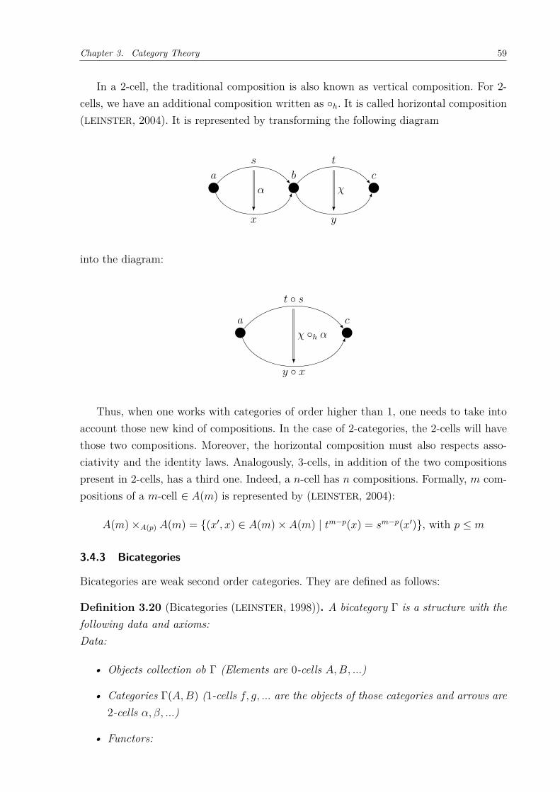
Chapter 3. Category Theory 59
In a 2-cell, the traditional composition is also known as vertical composition. For 2-cells, we have an additional composition written as ∘ℎ. It is called horizontal composition(LEINSTER, 2004). It is represented by transforming the following diagram
𝑎 𝑏 𝑐
𝑠
𝑥
𝑡
𝑦
𝛼 𝜒
into the diagram:
𝑎 𝑐
𝑡 ∘ 𝑠
𝑦 ∘ 𝑥
𝜒 ∘ℎ 𝛼
Thus, when one works with categories of order higher than 1, one needs to take intoaccount those new kind of compositions. In the case of 2-categories, the 2-cells will havethose two compositions. Moreover, the horizontal composition must also respects asso-ciativity and the identity laws. Analogously, 3-cells, in addition of the two compositionspresent in 2-cells, has a third one. Indeed, a 𝑛-cell has 𝑛 compositions. Formally, 𝑚 com-positions of a 𝑚-cell ∈ 𝐴(𝑚) is represented by (LEINSTER, 2004):
𝐴(𝑚) ×𝐴(𝑝) 𝐴(𝑚) = {(𝑥′, 𝑥) ∈ 𝐴(𝑚) × 𝐴(𝑚) | 𝑡𝑚−𝑝(𝑥) = 𝑠𝑚−𝑝(𝑥′)}, with 𝑝 ≤ 𝑚
3.4.3 Bicategories
Bicategories are weak second order categories. They are defined as follows:
Definition 3.20 (Bicategories (LEINSTER, 1998)). A bicategory Γ is a structure with thefollowing data and axioms:Data:
• Objects collection ob Γ (Elements are 0-cells 𝐴,𝐵, ...)
• Categories Γ(𝐴,𝐵) (1-cells 𝑓, 𝑔, ... are the objects of those categories and arrows are2-cells 𝛼, 𝛽, ...)
• Functors:

Chapter 3. Category Theory 60
𝑐𝐴𝐵𝐶 : Γ(𝐵,𝐶) × Γ(𝐴,𝐵) → Γ(𝐴,𝐶)
(𝑔, 𝑓) → 𝑔 ∘ 𝑓 = 𝑔𝑓
(𝛽, 𝛼) → 𝛽 ∘ℎ 𝛼
and 𝐼𝐴 : 1 → Γ(𝐴,𝐴) (thus, 𝐼𝐴 is an 1-cell 𝐴 → 𝐴)
• The following natural isomorphisms:
Thus, we have 2-cells:
𝑎ℎ𝑔𝑓 : (ℎ𝑔)𝑓 ∼−→ ℎ(𝑔𝑓)
𝑟𝑓 : 𝑓 ∘ 𝐼𝐴∼−→ 𝑓
𝑙𝑓 : 𝐼𝐵 ∘ 𝑓 ∼−→ 𝑓
Axioms:Consider the following configuration of 1-cells
𝑎 𝑏 𝑐 𝑑 𝑒𝑠 𝑟 𝑝 𝑢
The following diagrams commute:

Chapter 3. Category Theory 61
((𝑢 ∘ 𝑝) ∘ 𝑟) ∘ 𝑠
(𝑢 ∘ 𝑝) ∘ (𝑟 ∘ 𝑠)
(𝑢 ∘ (𝑝 ∘ 𝑟)) ∘ 𝑠
𝑢 ∘ ((𝑝 ∘ 𝑟) ∘ 𝑠)
𝑢 ∘ (𝑝 ∘ (𝑟 ∘ 𝑠))
𝑎
𝑎 ∘ℎ 1
𝑎
𝑎 1 ∘ℎ 𝑎
(𝑟 ∘ 𝜌𝑏) ∘ 𝑠 𝑟 ∘ (𝜌𝑏 ∘ 𝑠)
𝑟 ∘ 𝑠
𝑎
𝑟𝑟 ∘ℎ 1 1 ∘ℎ 𝑙𝑠
In the literature of higher order category theory, the axioms of a weak higher ordercategory are called coherence laws (LEINSTER, 2004).
3.5 CONCLUSION
In this chapter, we have seen the basic concepts of category theory. Most will play animportant role in the next chapter. The concepts of isomorphism and groupoid, for in-stance, will be the base for mathematical model for computational paths. We have alsoseen concepts of higher category theory, since in the sequel we are going to show thatcomputational paths forms a higher structure.

62
4 COMPUTATIONAL PATHS
In this chapter, we introduce the main concept of this work, an entity known ascomputational paths. In chapter 2, we have seen that it is possible to interpret theidentity type semantically, considering the terms as homotopical paths between two pointsof a space. Nevertheless, there is no entity that represents those paths in the syntax oftype theory. Thus, we add computational paths to fill this gap. In this sense, our objectiveis to formulate the identity type using this new entity.
This work has also been motivated by the fact that although beautifully defined, wehave noticed that proofs that uses the identity type can be sometimes a little too complex.The elimination rule of the intensional identity type encapsulates lots of information,sometimes making too troublesome the process of finding the reason that builds the correcttype. We have also seen this in chapter 2. We proposed constructions for the symmetryand transitivity of the identity type. Although one could expect those constructions to bepretty straightforward, the process of obtaining the right reason to construct those typeswas troublesome.
Thus, inspired by the path-based approach of the homotopy interpretation, we believethat a similar approach can be used to define the identity type in type theory. To achievethat, we have been using a notion of computational paths. The interpretation will besimilar to the homotopy one: a term 𝑝 : 𝐼𝑑𝐴(𝑎, 𝑏) will be a computational path betweenterms 𝑎, 𝑏 : 𝐴, and such path will be the result of a sequence of rewrites. In the sequel, weshall define formally the concept of a computational path. The main idea, i.e. proofs ofequality statements as (reversible) sequences of rewrites, is not new, as it goes back to apaper entitled “Equality in labeled deductive systems and the functional interpretation ofpropositional equality ", presented in December 1993 at the 9th Amsterdam Colloquium,and published in the proceedings in 1994(QUEIROZ; GABBAY, 1994).
In the previous chapter, we have seen the concept of higher structures such as highercategories. Indeed, one of the most interesting aspects of the identity type is the fact that itcan be used to construct higher structures. This is a rather natural consequence of the factthat it is possible to construct higher identities. For any 𝑎, 𝑏 : 𝐴, we have type 𝐼𝑑𝐴(𝑎, 𝑏). Ifthis type is inhabited by any 𝑝, 𝑞 : 𝐼𝑑𝐴(𝑎, 𝑏), then we have type 𝐼𝑑𝐼𝑑𝐴(𝑎,𝑏)(𝑝, 𝑞). If the lattertype is inhabited, we have a higher equality between 𝑝 and 𝑞(HARPER, 2012). This conceptis also present in computational paths. One can show the equality between two computa-tional paths 𝑠 and 𝑡 by constructing a third one between 𝑠 and 𝑡. We show in this chapter a
This chapter is based on two papers published by the author (jointly with his advisor and co-advisor):Propositional equality, identity types, and computational paths in South American Joournal of Logic,2016 (QUEIROZ; OLIVEIRA; RAMOS, 2016) and On the Identity Type as the Type of ComputationalPaths in Logic Journal of the IGPL, 2017 (RAMOS; QUEIROZ; OLIVEIRA, 2017).

Chapter 4. Computational Paths 63
system of rules used to establish equalities between computational paths(OLIVEIRA, 1995).Then, we show that these higher equalities go up to the infinity, forming a ∞-globular-set.We also show that computational paths naturally induce a groupoid structure. We alsogo a step further, showing that computational paths are capable of inducing a highergroupoid structure.
Another important question we want to answer is one that arises naturally whentalking about equality: Is there a canonical proof for an expression 𝑡1 = 𝑡2? In the languageof computational paths, is there a normal path between 𝑡1 = 𝑡2 such that every other pathcan be reduced to this one? In fact, we are going to prove that the answer is negative.Our model also refute the Uniquiness of Identity Proofs (UIP)).
4.1 INTRODUCING COMPUTATIONAL PATHS
Before we enter in details of computational paths, let’s recall what motivated the intro-duction of computational paths to type theory. In type theory, our types are interpretedusing the so-called Brower-Heyting-Kolmogorov Interpretation. That way, a semantic in-terpretation of types are not given by truth-values, but by the concept of proof as aprimitive notion. Thus, we have (QUEIROZ; OLIVEIRA; RAMOS, 2016):
a proof of the proposition: is given by:𝐴 ∧𝐵 a proof of 𝐴 and a proof of 𝐵𝐴 ∨𝐵 a proof of 𝐴 or a proof of 𝐵𝐴 → 𝐵 a function that turns a proof of 𝐴 into a proof of 𝐵∀𝑥𝐷.𝑃 (𝑥) a function that turns an element 𝑎 into a proof of 𝑃 (𝑎)∃𝑥𝐷.𝑃 (𝑥) an element 𝑎 (witness) and a proof of 𝑃 (𝑎)
Also, based on the Curry-Howard functional interpretation of logical connectives, onehave (QUEIROZ; OLIVEIRA; RAMOS, 2016):
a proof of the proposition: has the canonical form of:𝐴 ∧𝐵 ⟨𝑝, 𝑞⟩ where 𝑝 is a proof of 𝐴 and 𝑞 is a proof of 𝐵𝐴 ∨𝐵 𝑖(𝑝) where 𝑝 is a proof of 𝐴 or 𝑗(𝑞) where 𝑞 is a proof of 𝐵
(‘𝑖’ and ‘𝑗’ abbreviate ‘into the left/right disjunct’)𝐴 → 𝐵 𝜆𝑥.𝑏(𝑥) where 𝑏(𝑝) is a proof of B
provided 𝑝 is a proof of A∀𝑥𝐴.𝐵(𝑥) Λ𝑥.𝑓(𝑥) where 𝑓(𝑎) is a proof of 𝐵(𝑎)
provided 𝑎 is an arbitrary individual chosenfrom the domain 𝐴
∃𝑥𝐴.𝐵(𝑥) 𝜀𝑥.(𝑓(𝑥), 𝑎) where 𝑎 is a witnessfrom the domain 𝐴, 𝑓(𝑎) is a proof of 𝐵(𝑎)

Chapter 4. Computational Paths 64
If one looks closely, there is one interpretation missing in the BHK-Interpretation.What constitutes a proof of 𝑡1 = 𝑡2? In other words, what is a proof of an equalitystatement? We answer this by proposing that an equality between those two terms shouldbe a sequence of rewrites starting from 𝑡1 and ending at 𝑡2. Thus, we would have (QUEIROZ;
OLIVEIRA; RAMOS, 2016):
a proof of the proposition: is given by:
𝑡1 = 𝑡2 ?(Perhaps a sequence of rewritesstarting from 𝑡1 and ending in 𝑡2?)
We call computational path the sequence of rewrites between these terms.
4.1.1 Formal Definition
Since computational path is a generic term, it is important to emphasize the fact thatwe are using the term computational path in the sense defined by(QUEIROZ; OLIVEIRA,2014a). A computational path is based on the idea that it is possible to formally definewhen two computational objects 𝑎, 𝑏 : 𝐴 are equal. These two objects are equal if one canreach 𝑏 from 𝑎 by applying a sequence of axioms or rules. This sequence of operationsforms a path. Since it is between two computational objects, it is said that this path isa computational one. Also, an application of an axiom or a rule transforms (or rewrite)an term in another. For that reason, a computational path is also known as a sequenceof rewrites. Nevertheless, before we define formally a computational path, we can take alook at one famous equality theory, the 𝜆𝛽𝜂 − 𝑒𝑞𝑢𝑎𝑙𝑖𝑡𝑦(HINDLEY; SELDIN, 2008):
Definition 4.1. The 𝜆𝛽𝜂-equality is composed by the following axioms:
(𝛼) 𝜆𝑥.𝑀 = 𝜆𝑦.𝑀 [𝑦/𝑥] if 𝑦 /∈ 𝐹𝑉 (𝑀);
(𝛽) (𝜆𝑥.𝑀)𝑁 = 𝑀 [𝑁/𝑥];
(𝜌) 𝑀 = 𝑀 ;
(𝜂) (𝜆𝑥.𝑀𝑥) = 𝑀 (𝑥 /∈ 𝐹𝑉 (𝑀)).
And the following rules of inference:
𝑀 = 𝑀 ′(𝜇)
𝑁𝑀 = 𝑁𝑀 ′𝑀 = 𝑁 𝑁 = 𝑃(𝜏)
𝑀 = 𝑃

Chapter 4. Computational Paths 65
𝑀 = 𝑀 ′(𝜈)
𝑀𝑁 = 𝑀 ′𝑁𝑀 = 𝑁(𝜎)𝑁 = 𝑀
𝑀 = 𝑀 ′(𝜉)
𝜆𝑥.𝑀 = 𝜆𝑥.𝑀 ′
Definition 4.2. (HINDLEY; SELDIN, 2008) 𝑃 is 𝛽-equal or 𝛽-convertible to 𝑄 (notation𝑃 =𝛽 𝑄) iff 𝑄 is obtained from 𝑃 by a finite (perhaps empty) series of 𝛽-contractionsand reversed 𝛽-contractions and changes of bound variables. That is, 𝑃 =𝛽 𝑄 iff thereexist 𝑃0, . . . , 𝑃𝑛 (𝑛 ≥ 0) such that 𝑃0 ≡ 𝑃 , 𝑃𝑛 ≡ 𝑄, (∀𝑖 ≤ 𝑛− 1)(𝑃𝑖 ◁1𝛽 𝑃𝑖+1 or 𝑃𝑖+1 ◁1𝛽
𝑃𝑖 or 𝑃𝑖 ≡𝛼 𝑃𝑖+1).
(Note that equality has an existential force, which will show in the proof rules for theidentity type.)
The same happens with 𝜆𝛽𝜂-equality:
Definition 4.3. (𝜆𝛽𝜂-equality(HINDLEY; SELDIN, 2008)) The equality-relation determinedby the theory 𝜆𝛽𝜂 is called =𝛽𝜂; that is, we define
𝑀 =𝛽𝜂 𝑁 ⇔ 𝜆𝛽𝜂 ⊢ 𝑀 = 𝑁.
Example 4.1. Take the term 𝑀 ≡ (𝜆𝑥.(𝜆𝑦.𝑦𝑥)(𝜆𝑤.𝑧𝑤))𝑣. Then, it is 𝛽𝜂-equal to 𝑁 ≡ 𝑧𝑣
because of the sequence:(𝜆𝑥.(𝜆𝑦.𝑦𝑥)(𝜆𝑤.𝑧𝑤))𝑣, (𝜆𝑥.(𝜆𝑦.𝑦𝑥)𝑧)𝑣, (𝜆𝑦.𝑦𝑣)𝑧, 𝑧𝑣
which starts from 𝑀 and ends with 𝑁 , and each member of the sequence is obtained via1-step 𝛽- or 𝜂-contraction of a previous term in the sequence. To take this sequence intoa path, one has to apply transitivity twice, as we do in the example below.
Example 4.2. The term 𝑀 ≡ (𝜆𝑥.(𝜆𝑦.𝑦𝑥)(𝜆𝑤.𝑧𝑤))𝑣 is 𝛽𝜂-equal to 𝑁 ≡ 𝑧𝑣 because ofthe sequence:(𝜆𝑥.(𝜆𝑦.𝑦𝑥)(𝜆𝑤.𝑧𝑤))𝑣, (𝜆𝑥.(𝜆𝑦.𝑦𝑥)𝑧)𝑣, (𝜆𝑦.𝑦𝑣)𝑧, 𝑧𝑣
Now, taking this sequence into a path leads us to the following:The first is equal to the second based on the grounds:𝜂((𝜆𝑥.(𝜆𝑦.𝑦𝑥)(𝜆𝑤.𝑧𝑤))𝑣, (𝜆𝑥.(𝜆𝑦.𝑦𝑥)𝑧)𝑣)The second is equal to the third based on the grounds:𝛽((𝜆𝑥.(𝜆𝑦.𝑦𝑥)𝑧)𝑣, (𝜆𝑦.𝑦𝑣)𝑧)Now, the first is equal to the third based on the grounds:𝜏(𝜂((𝜆𝑥.(𝜆𝑦.𝑦𝑥)(𝜆𝑤.𝑧𝑤))𝑣, (𝜆𝑥.(𝜆𝑦.𝑦𝑥)𝑧)𝑣), 𝛽((𝜆𝑥.(𝜆𝑦.𝑦𝑥)𝑧)𝑣, (𝜆𝑦.𝑦𝑣)𝑧))Now, the third is equal to the fourth one based on the grounds:𝛽((𝜆𝑦.𝑦𝑣)𝑧, 𝑧𝑣)Thus, the first one is equal to the fourth one based on the grounds:𝜏(𝜏(𝜂((𝜆𝑥.(𝜆𝑦.𝑦𝑥)(𝜆𝑤.𝑧𝑤))𝑣, (𝜆𝑥.(𝜆𝑦.𝑦𝑥)𝑧)𝑣), 𝛽((𝜆𝑥.(𝜆𝑦.𝑦𝑥)𝑧)𝑣, (𝜆𝑦.𝑦𝑣)𝑧)), 𝛽((𝜆𝑦.𝑦𝑣)𝑧, 𝑧𝑣))).

Chapter 4. Computational Paths 66
The aforementioned theory establishes the equality between two 𝜆-terms. Since weare working with computational objects as terms of a type, we need to translate the𝜆𝛽𝜂-equality to a suitable equality theory based on Martin Löf’s type theory. We obtain:
Definition 4.4. The equality theory of Martin Löf’s type theory has the following basicproof rules for the Π-type:
𝑁 : 𝐴[𝑥 : 𝐴]𝑀 : 𝐵(𝛽) (𝜆𝑥.𝑀)𝑁 = 𝑀 [𝑁/𝑥] : 𝐵[𝑁/𝑥]
[𝑥 : 𝐴]𝑀 = 𝑀 ′ : 𝐵(𝜉)
𝜆𝑥.𝑀 = 𝜆𝑥.𝑀 ′ : (Π𝑥 : 𝐴)𝐵
𝑀 : 𝐴(𝜌)𝑀 = 𝑀 : 𝐴
𝑀 = 𝑀 ′ : 𝐴 𝑁 : (Π𝑥 : 𝐴)𝐵(𝜇)𝑁𝑀 = 𝑁𝑀 ′ : 𝐵[𝑀/𝑥]
𝑀 = 𝑁 : 𝐴(𝜎)𝑁 = 𝑀 : 𝐴
𝑁 : 𝐴 𝑀 = 𝑀 ′ : (Π𝑥 : 𝐴)𝐵(𝜈)𝑀𝑁 = 𝑀 ′𝑁 : 𝐵[𝑁/𝑥]
𝑀 = 𝑁 : 𝐴 𝑁 = 𝑃 : 𝐴(𝜏)𝑀 = 𝑃 : 𝐴
𝑀 : (Π𝑥 : 𝐴)𝐵(𝜂) (𝑥 /∈ 𝐹𝑉 (𝑀))(𝜆𝑥.𝑀𝑥) = 𝑀 : (Π𝑥 : 𝐴)𝐵
We are finally able to formally define computational paths:
Definition 4.5. Let 𝑎 and 𝑏 be elements of a type 𝐴. Then, a computational path 𝑠 from𝑎 to 𝑏 is a composition of rewrites (each rewrite is an application of the inference rules ofthe equality theory of type theory or is a change of bound variables). We denote that by𝑎 =𝑠 𝑏.
As we have seen in example 4.2, composition of rewrites are applications of the rule 𝜏 .Since change of bound variables is possible, each term is considered up to 𝛼-equivalence.
4.1.2 Equality Equations
One can use the aforementioned axioms to show that computational paths establishes thethree fundamental equations of equality: the reflexivity, symmetry and transitivity:
𝑎 =𝑡 𝑏 : 𝐴 𝑏 =𝑢 𝑐 : 𝐴 transitivity𝑎 =𝜏(𝑡,𝑢) 𝑐 : 𝐴
𝑎 : 𝐴 reflexivity𝑎 =𝜌 𝑎 : 𝐴
𝑎 =𝑡 𝑏 : 𝐴 symmetry𝑏 =𝜎(𝑡) 𝑎 : 𝐴

Chapter 4. Computational Paths 67
4.1.3 Identity Type
We have said that it is possible to formulate the identity type using computational paths.As we have seen, the best way to define any formal entity of type theory is by a set ofnatural deductions rules. Thus, we define our path-based approach as the following set ofrules:
• Formation and Introduction rules (QUEIROZ; OLIVEIRA; RAMOS, 2016; RAMOS; QUEIROZ;
OLIVEIRA, 2017):
𝐴 type 𝑎 : 𝐴 𝑏 : 𝐴𝐼𝑑− 𝐹
𝐼𝑑𝐴(𝑎, 𝑏) type
𝑎 =𝑠 𝑏 : 𝐴𝐼𝑑− 𝐼
𝑠(𝑎, 𝑏) : 𝐼𝑑𝐴(𝑎, 𝑏)
One can notice that our formation rule is exactly equal to the traditional identitytype. From terms 𝑎, 𝑏 : 𝐴, one can form that is inhabited only if there is a proof ofequality between those terms, i.e., 𝐼𝑑𝐴(𝑎, 𝑏).
The difference starts with the introduction rule. In our approach, one can noticethat we do not use a reflexive constructor 𝑟. In other words, the reflexive path is notthe main building block of our identity type. Instead, if we have a computationalpath 𝑎 =𝑠 𝑏 : 𝐴, we introduce 𝑠(𝑎, 𝑏) as a term of the identity type. That way, oneshould see 𝑠(𝑎, 𝑏) as a sequence of rewrites and substitutions (i.e., a computationalpath) which would have started from 𝑎 and arrived at 𝑏
• Elimination rule (QUEIROZ; OLIVEIRA; RAMOS, 2016; RAMOS; QUEIROZ; OLIVEIRA,2017):
𝑚 : 𝐼𝑑𝐴(𝑎, 𝑏)[𝑎 =𝑔 𝑏 : 𝐴]ℎ(𝑔) : 𝐶
𝐼𝑑− 𝐸𝑅𝐸𝑊𝑅(𝑚, 𝑔.ℎ(𝑔)) : 𝐶
Let’s recall the notation being used. First, one should see ℎ(𝑔) as a functionalexpression ℎ which depends on 𝑔. Also, one should notice the use of ‘́ ’ in 𝑔. Oneshould see ‘́ ’ as an abstractor that binds the occurrences of the variable 𝑔 introducedin the local assumption [𝑎 =𝑔 𝑏 : 𝐴] as a kind of Skolem-type constant denoting thereason why 𝑎 was assumed to be equal to 𝑏.
We also introduce the constructor 𝑅𝐸𝑊𝑅. In a sense, it is similar to the constructor𝐽 of the traditional approach, since both arise from the elimination rule of the

Chapter 4. Computational Paths 68
identity type. The behavior of 𝑅𝐸𝑊𝑅 is simple. If from a computational path 𝑔
that establishes the equality between 𝑎 and 𝑏 one can construct ℎ(𝑔) : 𝐶, then ifwe also have this equality established by a term 𝑚 : 𝐼𝑑𝐴(𝑎, 𝑏), we can put togetherall this information in 𝑅𝐸𝑊𝑅 to construct 𝐶, eliminating the type 𝐼𝑑𝐴(𝑎, 𝑏) in theprocess. The idea is that we can substitute 𝑔 for 𝑚 in 𝑔.ℎ(𝑔), resulting in ℎ(𝑚/𝑔) : 𝐶.This behavior is established next by the reduction rule.
• Reduction rule (QUEIROZ; OLIVEIRA; RAMOS, 2016; RAMOS; QUEIROZ; OLIVEIRA,2017):
𝑎 =𝑚 𝑏 : 𝐴𝐼𝑑− 𝐼
𝑚(𝑎, 𝑏) : 𝐼𝑑𝐴(𝑎, 𝑏)[𝑎 =𝑔 𝑏 : 𝐴]ℎ(𝑔) : 𝐶
𝐼𝑑− 𝐸 B𝛽𝑅𝐸𝑊𝑅(𝑚, 𝑔.ℎ(𝑔)) : 𝐶
[𝑎 =𝑚 𝑏 : 𝐴]ℎ(𝑚/𝑔) : 𝐶
• Induction rule:
𝑒 : 𝐼𝑑𝐴(𝑎, 𝑏)[𝑎 =𝑡 𝑏 : 𝐴]
𝐼𝑑− 𝐼𝑡(𝑎, 𝑏) : 𝐼𝑑𝐴(𝑎, 𝑏)
𝐼𝑑− 𝐸 B𝜂 𝑒 : 𝐼𝑑𝐴(𝑎, 𝑏)𝑅𝐸𝑊𝑅(𝑒, 𝑡.𝑡(𝑎, 𝑏)) : 𝐼𝑑𝐴(𝑎, 𝑏)
Our introduction and elimination rules reassure the concept of equality as an existen-tial force. In the introduction rule, we encapsulate the idea that a witness of a identitytype 𝐼𝑑𝐴(𝑎, 𝑏) only exists if there exist a computational path establishing the equality of𝑎 and 𝑏. Also, one can notice that our elimination rule is similar to the elimination ruleof the existential quantifier.
4.1.4 Path-based Examples
The objective of this subsection is to show how to use in practice the rules that we havejust defined. The idea is to show construction of terms of some important types. Theconstructions that we have chosen to build are the reflexive, transitive and symmetrictype of the identity type. Those were not random choices. The main reason is the factthat reflexive, transitive and symmetric types are essential to the process of buildinga groupoid model for the identity type(HOFMANN; STREICHER, 1994). As we shall see,these constructions come naturally from simple computational paths constructed by theapplication of axioms of the equality of type theory.
Before we start the constructions, we think that it is essential to understand how to usethe eliminations rules. The process of building a term of some type is a matter of findingthe right reason. In the case of 𝐽 , the reason is the correct 𝑥, 𝑦 : 𝐴 and 𝑧 : 𝐼𝑑𝐴(𝑎, 𝑏) thatgenerates the adequate 𝐶(𝑥, 𝑦, 𝑧). In our approach, the reason is the correct path 𝑎 =𝑔 𝑏
that generates the adequate 𝑔(𝑎, 𝑏) : 𝐼𝑑(𝑎, 𝑏).

Chapter 4. Computational Paths 69
4.1.4.1 Reflexivity
One could find strange the fact that we need to prove the reflexivity. Nevertheless, justremember that our approach is not based on the idea that reflexivity is the base of theidentity type. As usual in type theory, a proof of something comes down to a constructionof a term of a type. In this case, we need to construct a term of type Π(𝑎:𝐴)𝐼𝑑𝐴(𝑎, 𝑎).The reason is extremely simple: from a term 𝑎 : 𝐴, we obtain the computational path𝑎 =𝜌 𝑎 : 𝐴 (RAMOS; QUEIROZ; OLIVEIRA, 2017):
[𝑎 : 𝐴]𝑎 =𝜌 𝑎 : 𝐴
𝐼𝑑− 𝐼𝜌(𝑎, 𝑎) : 𝐼𝑑𝐴(𝑎, 𝑎)
Π − 𝐼𝜆𝑎.𝜌(𝑎, 𝑎) : Π(𝑎:𝐴)𝐼𝑑𝐴(𝑎, 𝑎)
4.1.4.2 Symmetry
The second proposed construction is the symmetry. Our objective is to obtain a term oftype Π(𝑎:𝐴)Π(𝑏:𝐴)(𝐼𝑑𝐴(𝑎, 𝑏) → 𝐼𝑑𝐴(𝑏, 𝑎)).
We construct a proof using computational paths. As expected, we need to find asuitable reason. Starting from 𝑎 =𝑡 𝑏, we could look at the axioms of definition 4.1 toplan our next step. One of those axioms makes the symmetry clear: the 𝜎 axiom. If weapply 𝜎, we will obtain 𝑏 =𝜎(𝑡) 𝑎. From this, we can then infer that 𝐼𝑑𝐴 is inhabitedby (𝜎(𝑡))(𝑏, 𝑎). Now, it is just a matter of applying the elimination (RAMOS; QUEIROZ;
OLIVEIRA, 2017):
[𝑎 : 𝐴] [𝑏 : 𝐴][𝑝(𝑎, 𝑏) : 𝐼𝑑𝐴(𝑎, 𝑏)]
[𝑎 =𝑡 𝑏 : 𝐴]𝑏 =𝜎(𝑡) 𝑎 : 𝐴
𝐼𝑑− 𝐼(𝜎(𝑡))(𝑏, 𝑎) : 𝐼𝑑𝐴(𝑏, 𝑎)𝐼𝑑− 𝐸
𝑅𝐸𝑊𝑅(𝑝(𝑎, 𝑏), 𝑡.(𝜎(𝑡))(𝑏, 𝑎)) : 𝐼𝑑𝐴(𝑏, 𝑎)→ −𝐼
𝜆𝑝.𝑅𝐸𝑊𝑅(𝑝(𝑎, 𝑏), 𝑡.(𝜎(𝑡))(𝑏, 𝑎)) : 𝐼𝑑𝐴(𝑎, 𝑏) → 𝐼𝑑𝐴(𝑏, 𝑎)Π − 𝐼
𝜆𝑏.𝜆𝑝.𝑅𝐸𝑊𝑅(𝑝(𝑎, 𝑏), 𝑡.(𝜎(𝑡))(𝑏, 𝑎)) : Π(𝑏:𝐴)(𝐼𝑑𝐴(𝑎, 𝑏) → 𝐼𝑑𝐴(𝑏, 𝑎))Π − 𝐼
𝜆𝑎.𝜆𝑏.𝜆𝑝.𝑅𝐸𝑊𝑅(𝑝(𝑎, 𝑏), 𝑡.(𝜎(𝑡))(𝑏, 𝑎)) : Π(𝑎:𝐴)Π(𝑏:𝐴)(𝐼𝑑𝐴(𝑎, 𝑏) → 𝐼𝑑𝐴(𝑏, 𝑎))
4.1.4.3 Transitivity
The third and last construction will be the transitivity. Our objective os to obtain a termof type Π(𝑎:𝐴)Π(𝑏:𝐴)Π(𝑐:𝐴)(𝐼𝑑𝐴(𝑎, 𝑏) → 𝐼𝑑𝐴(𝑏, 𝑐) → 𝐼𝑑𝐴(𝑎, 𝑐)).
To build our path-based construction, the first step, as expected, is to find the reason.Since we are trying to construct the transitivity, it is natural to think that we should start

Chapter 4. Computational Paths 70
with paths 𝑎 =𝑡 𝑏 and 𝑏 =𝑢 𝑐 and then, from these paths, we should conclude that thereis a path 𝑧 that establishes that 𝑎 =𝑧 𝑐. To obtain 𝑧, we could try to apply the axiomsof definition 4.1. Looking at the axioms, one is exactly what we want: the axiom 𝜏 . Ifwe apply 𝜏 to 𝑎 =𝑡 𝑏 and 𝑏 =𝑢 𝑐, we will obtain a new path 𝜏(𝑡, 𝑢) such that 𝑎 =𝜏(𝑡,𝑢) 𝑐.Using that construction as the reason, we obtain the following term (RAMOS; QUEIROZ;
OLIVEIRA, 2017):

Chapter 4. Computational Paths 71
[𝑎:𝐴
][𝑏
:𝐴]
[𝑤(𝑎,𝑏
):𝐼𝑑
𝐴(𝑎,𝑏
)]
[𝑐:𝐴
][𝑠
(𝑏,𝑐
):𝐼𝑑
𝐴(𝑏,𝑐
)]
[𝑎=
𝑡𝑏
:𝐴]
[𝑏=
𝑢𝑐
:𝐴]
𝑎=
𝜏(𝑡
,𝑢)𝑐
:𝐴𝐼𝑑
−𝐼
(𝜏(𝑡,𝑢
))(𝑎,𝑐
):𝐼𝑑
𝐴(𝑎,𝑐
)𝐼𝑑
−𝐸
𝑅𝐸𝑊𝑅
(𝑠(𝑏,𝑐
),𝑢(𝜏
(𝑡,𝑢
))(𝑎,𝑐
)):𝐼𝑑
𝐴(𝑎,𝑐
)𝐼𝑑
−𝐸
𝑅𝐸𝑊𝑅
(𝑤(𝑎,𝑏
),𝑡𝑅𝐸𝑊𝑅
(𝑠(𝑏,𝑐
),𝑢(𝜏
(𝑡,𝑢
))(𝑎,𝑐
))):𝐼𝑑
𝐴(𝑎,𝑐
)→
−𝐼
𝜆𝑠.𝑅𝐸𝑊𝑅
(𝑤(𝑎,𝑏
),𝑡𝑅𝐸𝑊𝑅
(𝑠(𝑏,𝑐
),𝑢(𝜏
(𝑡,𝑢
))(𝑎,𝑐
))):𝐼𝑑
𝐴(𝑏,𝑐
)→𝐼𝑑
𝐴(𝑎,𝑐
)→
−𝐼
𝜆𝑤.𝜆𝑠.𝑅𝐸𝑊𝑅
(𝑤(𝑎,𝑏
),𝑡𝑅𝐸𝑊𝑅
(𝑠(𝑏,𝑐
),𝑢(𝜏
(𝑡,𝑢
))(𝑎,𝑐
))):𝐼𝑑
𝐴(𝑎,𝑏
)→𝐼𝑑
𝐴(𝑏,𝑐
)→𝐼𝑑
𝐴(𝑎,𝑐
)Π
−𝐼
𝜆𝑐.𝜆𝑤.𝜆𝑠.𝑅𝐸𝑊𝑅
(𝑤(𝑎,𝑏
),𝑡𝑅𝐸𝑊𝑅
(𝑠(𝑏,𝑐
),𝑢(𝜏
(𝑡,𝑢
))(𝑎,𝑐
))):
Π(𝑐
:𝐴)(𝐼𝑑
𝐴(𝑎,𝑏
)→𝐼𝑑
𝐴(𝑏,𝑐
)→𝐼𝑑
𝐴(𝑎,𝑐
))Π
−𝐼
𝜆𝑏.𝜆𝑐.𝜆𝑤.𝜆𝑠.𝑅𝐸𝑊𝑅
(𝑤(𝑎,𝑏
),𝑡𝑅𝐸𝑊𝑅
(𝑠(𝑏,𝑐
),𝑢(𝜏
(𝑡,𝑢
))(𝑎,𝑐
))):
Π(𝑏
:𝐴)Π
(𝑐:𝐴
)(𝐼𝑑
𝐴(𝑎,𝑏
)→𝐼𝑑
𝐴(𝑏,𝑐
)→𝐼𝑑
𝐴(𝑎,𝑐
))Π
−𝐼
𝜆𝑎.𝜆𝑏.𝜆𝑐.𝜆𝑤.𝜆𝑠.𝑅𝐸𝑊𝑅
(𝑤(𝑎,𝑏
),𝑡𝑅𝐸𝑊𝑅
(𝑠(𝑏,𝑐
),𝑢(𝜏
(𝑡,𝑢
))(𝑎,𝑐
))):
Π(𝑎
:𝐴)Π
(𝑏:𝐴
)Π(𝑐
:𝐴)(𝐼𝑑
𝐴(𝑎,𝑏
)→𝐼𝑑
𝐴(𝑏,𝑐
)→𝐼𝑑
𝐴(𝑎,𝑐
))
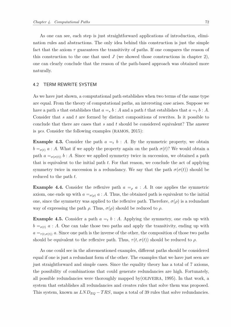
Chapter 4. Computational Paths 72
As one can see, each step is just straightforward applications of introduction, elimi-nation rules and abstractions. The only idea behind this construction is just the simplefact that the axiom 𝜏 guarantees the transitivity of paths. If one compares the reason ofthis construction to the one that used 𝐽 (we showed those constructions in chapter 2),one can clearly conclude that the reason of the path-based approach was obtained morenaturally.
4.2 TERM REWRITE SYSTEM
As we have just shown, a computational path establishes when two terms of the same typeare equal. From the theory of computational paths, an interesting case arises. Suppose wehave a path 𝑠 that establishes that 𝑎 =𝑠 𝑏 : 𝐴 and a path 𝑡 that establishes that 𝑎 =𝑡 𝑏 : 𝐴.Consider that 𝑠 and 𝑡 are formed by distinct compositions of rewrites. Is it possible toconclude that there are cases that 𝑠 and 𝑡 should be considered equivalent? The answeris yes. Consider the following examples (RAMOS, 2015):
Example 4.3. Consider the path 𝑎 =𝑡 𝑏 : 𝐴. By the symmetric property, we obtain𝑏 =𝜎(𝑡) 𝑎 : 𝐴. What if we apply the property again on the path 𝜎(𝑡)? We would obtain apath 𝑎 =𝜎(𝜎(𝑡)) 𝑏 : 𝐴. Since we applied symmetry twice in succession, we obtained a paththat is equivalent to the initial path 𝑡. For that reason, we conclude the act of applyingsymmetry twice in succession is a redundancy. We say that the path 𝜎(𝜎(𝑡)) should bereduced to the path 𝑡.
Example 4.4. Consider the reflexive path 𝑎 =𝜌 𝑎 : 𝐴. It one applies the symmetricaxiom, one ends up with 𝑎 =𝜎(𝜌) 𝑎 : 𝐴. Thus, the obtained path is equivalent to the initialone, since the symmetry was applied to the reflexive path. Therefore, 𝜎(𝜌) is a redundantway of expressing the path 𝜌. Thus, 𝜎(𝜌) should be reduced to 𝜌.
Example 4.5. Consider a path 𝑎 =𝑡 𝑏 : 𝐴. Applying the symmetry, one ends up with𝑏 =𝜎(𝑡) 𝑎 : 𝐴. One can take those two paths and apply the transitivity, ending up with𝑎 =𝜏(𝑡,𝜎(𝑡)) 𝑎. Since one path is the inverse of the other, the composition of those two pathsshould be equivalent to the reflexive path. Thus, 𝜏(𝑡, 𝜎(𝑡)) should be reduced to 𝜌.
As one could see in the aforementioned examples, different paths should be consideredequal if one is just a redundant form of the other. The examples that we have just seen arejust straightforward and simple cases. Since the equality theory has a total of 7 axioms,the possibility of combinations that could generate redundancies are high. Fortunately,all possible redundancies were thoroughly mapped by(OLIVEIRA, 1995). In that work, asystem that establishes all redundancies and creates rules that solve them was proposed.This system, known as 𝐿𝑁𝐷𝐸𝑄 −𝑇𝑅𝑆, maps a total of 39 rules that solve redundancies.

Chapter 4. Computational Paths 73
4.2.1 𝐿𝑁𝐷𝐸𝑄 − 𝑇𝑅𝑆
In this subsection, we show the rules that compose the 𝐿𝑁𝐷𝐸𝑄 − 𝑇𝑅𝑆. All those rulescomes from the mapping of redundancies between computational paths, as we have seenin the 3 previous examples.
4.2.1.1 Subterm Substitution
Before we introduce the rewriting rules, it is important to introduce the concept of subtermsubstitution. In Equational Logic, the subterm substitution is given by the followinginference rule(OLIVEIRA; QUEIROZ, 1994):
𝑠 = 𝑡𝑠𝜃 = 𝑡𝜃
One problem is that such rule does not respect the sub-formula property. To deal withthat,(CHENADEC, 1989) proposes two inference rules:
𝑀 = 𝑁 𝐶[𝑁 ] = 𝑂𝐼𝐿
𝐶[𝑀 ] = 𝑂
𝑀 = 𝐶[𝑁 ] 𝑁 = 𝑂𝐼𝑅
𝑀 = 𝐶[𝑂]
where M, N and O are terms.As proposed in (QUEIROZ; OLIVEIRA; RAMOS, 2016), we can define similar rules using
computational paths, as follows:
𝑥 =𝑟 𝒞[𝑦] : 𝐴 𝑦 =𝑠 𝑢 : 𝐴′
𝑥 =subL(𝑟,𝑠) 𝒞[𝑢] : 𝐴𝑥 =𝑟 𝑤 : 𝐴′ 𝒞[𝑤] =𝑠 𝑢 : 𝐴
𝒞[𝑥] =subR(𝑟,𝑠) 𝑢 : 𝐴
where 𝐶 is the context in which the sub-term detached by ’[ ]’ appears and 𝐴′ could bea sub-domain of 𝐴, equal to 𝐴 or disjoint to 𝐴.
In the rule above, 𝒞[𝑢] should be understood as the result of replacing every occurrenceof 𝑦 by 𝑢 in 𝐶.
4.2.1.2 Rewriting Rules
In this subsection, our objective is to show all rewrite reductions and their associatedrewriting rules. The idea is to analyze all possible occurrences of redundancies in proofswhich involves the rules of rewritings.
We start with the transitivity:
Definition 4.6 (reductions involving 𝜏 (QUEIROZ; OLIVEIRA; RAMOS, 2016)).
𝑥 =𝑟 𝑦 : 𝐴 𝑦 =𝜎(𝑟) 𝑥 : 𝐴𝑥 =𝜏(𝑟,𝜎(𝑟)) 𝑥 : 𝐴 ◁𝑡𝑟 𝑥 =𝜌 𝑥 : 𝐴
𝑦 =𝜎(𝑟) 𝑥 : 𝐴 𝑥 =𝑟 𝑦 : 𝐴𝑦 =𝜏(𝜎(𝑟),𝑟) 𝑦 : 𝐴 ◁𝑡𝑠𝑟 𝑦 =𝜌 𝑦 : 𝐴

Chapter 4. Computational Paths 74
𝑢 =𝑟 𝑣 : 𝐴 𝑣 =𝜌 𝑣 : 𝐴𝑢 =𝜏(𝑟,𝜌) 𝑣 : 𝐴 ◁𝑡𝑟𝑟 𝑢 =𝑟 𝑣 : 𝐴
𝑢 =𝜌 𝑢 : 𝐴 𝑢 =𝑟 𝑣 : 𝐴𝑢 =𝜏(𝜌,𝑟) 𝑣 : 𝐴 ◁𝑡𝑙𝑟 𝑢 =𝑟 𝑣 : 𝐴
Associated rewriting rules:𝜏(𝑟, 𝜎(𝑟)) ◁𝑡𝑟 𝜌
𝜏(𝜎(𝑟), 𝑟) ◁𝑡𝑠𝑟 𝜌
𝜏(𝑟, 𝜌) ◁𝑡𝑟𝑟 𝑟
𝜏(𝜌, 𝑟) ◁𝑡𝑙𝑟 𝑟.
These reductions can be generalized to transformations where the reasons 𝑟 and 𝜎(𝑟)(transf. 1 and 2) and 𝑟 and 𝜌 (transf. 3 and 4) appear in some context, as illustrated bythe following example: (QUEIROZ; OLIVEIRA; RAMOS, 2016):
Example 4.6.
𝑥 =𝑟 𝑦 : 𝐴𝑖(𝑥) =𝜉1(𝑟) 𝑖(𝑦) : 𝐴+𝐵
𝑥 =𝑟 𝑦 : 𝐴𝑦 =𝜎(𝑟) 𝑥 : 𝐴
𝑖(𝑦) =𝜉1(𝜎(𝑟)) 𝑖(𝑥) : 𝐴+𝐵
𝑖(𝑥) =𝜏(𝜉1(𝑟),𝜉1(𝜎(𝑟))) 𝑖(𝑥) : 𝐴+𝐵
◁𝑡𝑟𝑥 =𝑟 𝑦 : 𝐴
𝑖(𝑥) =𝜉1(𝑟) 𝑖(𝑦) : 𝐴+𝐵
Associated rewriting:𝜏(𝜉1(𝑟), 𝜉1(𝜎(𝑟))) ◁𝑡𝑟 𝜉1(𝑟).
For the general context 𝒞[ ]:Associated rewritings:𝜏(𝒞[𝑟], 𝒞[𝜎(𝑟)]) ◁𝑡𝑟 𝒞[𝜌]𝜏(𝒞[𝜎(𝑟)], 𝒞[𝑟]) ◁𝑡𝑠𝑟 𝒞[𝜌]𝜏(𝒞[𝑟], 𝒞[𝜌]) ◁𝑡𝑟𝑟 𝒞[𝑟]𝜏(𝒞[𝜌], 𝒞[𝑟]) ◁𝑡𝑙𝑟 𝒞[𝑟]
The transitivity rules are pretty straightforward. We have more complicated cases(QUEIROZ; OLIVEIRA; RAMOS, 2016):
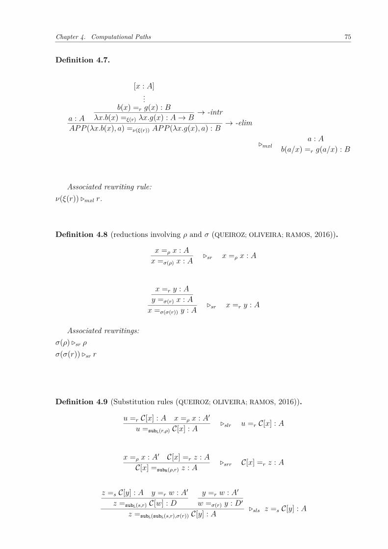
Chapter 4. Computational Paths 75
Definition 4.7.
𝑎 : 𝐴
[𝑥 : 𝐴]...
𝑏(𝑥) =𝑟 𝑔(𝑥) : 𝐵𝜆𝑥.𝑏(𝑥) =𝜉(𝑟) 𝜆𝑥.𝑔(𝑥) : 𝐴 → 𝐵
→ -intr
𝐴𝑃𝑃 (𝜆𝑥.𝑏(𝑥), 𝑎) =𝜈(𝜉(𝑟)) 𝐴𝑃𝑃 (𝜆𝑥.𝑔(𝑥), 𝑎) : 𝐵 → -elim
◁𝑚𝑥𝑙𝑎 : 𝐴
𝑏(𝑎/𝑥) =𝑟 𝑔(𝑎/𝑥) : 𝐵
Associated rewriting rule:𝜈(𝜉(𝑟)) ◁𝑚𝑥𝑙 𝑟.
Definition 4.8 (reductions involving 𝜌 and 𝜎 (QUEIROZ; OLIVEIRA; RAMOS, 2016)).
𝑥 =𝜌 𝑥 : 𝐴𝑥 =𝜎(𝜌) 𝑥 : 𝐴 ◁𝑠𝑟 𝑥 =𝜌 𝑥 : 𝐴
𝑥 =𝑟 𝑦 : 𝐴𝑦 =𝜎(𝑟) 𝑥 : 𝐴𝑥 =𝜎(𝜎(𝑟)) 𝑦 : 𝐴 ◁𝑠𝑟 𝑥 =𝑟 𝑦 : 𝐴
Associated rewritings:𝜎(𝜌) ◁𝑠𝑟 𝜌
𝜎(𝜎(𝑟)) ◁𝑠𝑟 𝑟
Definition 4.9 (Substitution rules (QUEIROZ; OLIVEIRA; RAMOS, 2016)).
𝑢 =𝑟 𝒞[𝑥] : 𝐴 𝑥 =𝜌 𝑥 : 𝐴′
𝑢 =subL(𝑟,𝜌) 𝒞[𝑥] : 𝐴 ◁𝑠𝑙𝑟 𝑢 =𝑟 𝒞[𝑥] : 𝐴
𝑥 =𝜌 𝑥 : 𝐴′ 𝒞[𝑥] =𝑟 𝑧 : 𝐴𝒞[𝑥] =subR(𝜌,𝑟) 𝑧 : 𝐴 ◁𝑠𝑟𝑟 𝒞[𝑥] =𝑟 𝑧 : 𝐴
𝑧 =𝑠 𝒞[𝑦] : 𝐴 𝑦 =𝑟 𝑤 : 𝐴′
𝑧 =subL(𝑠,𝑟) 𝒞[𝑤] : 𝐷𝑦 =𝑟 𝑤 : 𝐴′
𝑤 =𝜎(𝑟) 𝑦 : 𝐷′
𝑧 =subL(subL(𝑠,𝑟),𝜎(𝑟)) 𝒞[𝑦] : 𝐴 ◁𝑠𝑙𝑠 𝑧 =𝑠 𝒞[𝑦] : 𝐴

Chapter 4. Computational Paths 76
𝑧 =𝑠 𝒞[𝑦] : 𝐴 𝑦 =𝑟 𝑤 : 𝐴′
𝑧 =subL(𝑠,𝑟) 𝒞[𝑤] : 𝐴𝑦 =𝑟 𝑤 : 𝐴′
𝑤 =𝜎(𝑟) 𝑦 : 𝐴′
𝑧 =subL(subL(𝑠,𝑟),𝜎(𝑟)) 𝒞[𝑦] : 𝐴 ◁𝑠𝑙𝑠𝑠 𝑧 =𝑠 𝒞[𝑦] : 𝐴
𝑥 =𝑠 𝑤 : 𝐴′
𝑥 =𝑠 𝑤 : 𝐴′
𝑤 =𝜎(𝑠) 𝑥 : 𝐴′ 𝒞[𝑥] =𝑟 𝑧 : 𝐴𝒞[𝑤] =subR(𝜎(𝑠),𝑟) 𝑧 : 𝐴
𝒞[𝑥] =subR(𝑠,subR(𝜎(𝑠),𝑟)) 𝑧 : 𝐴 ◁𝑠𝑟𝑠 𝒞[𝑥] =𝑟 𝑧 : 𝐴
𝑥 =𝑠 𝑤 : 𝐴′
𝑤 =𝜎(𝑠) 𝑥 : 𝐴′𝑥 =𝑠 𝑤 : 𝐴′ 𝒞[𝑤] =𝑟 𝑧 : 𝐴
𝒞[𝑥] =subR(𝑠,𝑟) 𝑧 : 𝐴𝒞[𝑤] =subR(𝜎(𝑠),subR(𝑠,𝑟)) 𝑧 : 𝐴 ◁𝑠𝑟𝑟𝑟 𝒞[𝑤] =𝑟 𝑧 : 𝐴
Associated rewritings:subL(𝒞[𝑟], 𝒞[𝜌]) ◁𝑠𝑙𝑟 𝒞[𝑟]subR(𝒞[𝜌], 𝒞[𝑟]) ◁𝑠𝑟𝑟 𝒞[𝑟]subL(subL(𝑠, 𝒞[𝑟]), 𝒞[𝜎(𝑟)]) ◁𝑠𝑙𝑠 𝑠
subL(subL(𝑠, 𝒞[𝜎(𝑟)]), 𝒞[𝑟]) ◁𝑠𝑙𝑠𝑠 𝑠
subR(𝑠, subR(𝒞[𝜎(𝑠)], 𝑟)) ◁𝑠𝑟𝑠 𝑟
subR(𝒞[𝜎(𝑠)], subR(𝒞[𝑠], 𝑟)) ◁𝑠𝑟𝑟𝑟 𝑟
Definition 4.10 ((QUEIROZ; OLIVEIRA; RAMOS, 2016)).
𝛽𝑟𝑒𝑤𝑟-×-reduction𝑥 =𝑟 𝑦 : 𝐴 𝑧 : 𝐵
⟨𝑥, 𝑧⟩ =𝜉1(𝑟) ⟨𝑦, 𝑧⟩ : 𝐴×𝐵× -intr
𝐹𝑆𝑇 (⟨𝑥, 𝑧⟩) =𝜇1(𝜉1(𝑟)) 𝐹𝑆𝑇 (⟨𝑦, 𝑧⟩) : 𝐴 × -elim
◁𝑚𝑥2𝑙 𝑥 =𝑟 𝑦 : 𝐴
𝑥 =𝑟 𝑥′ : 𝐴 𝑦 =𝑠 𝑧 : 𝐵
⟨𝑥, 𝑦⟩ =𝜉∧(𝑟,𝑠) ⟨𝑥′, 𝑧⟩ : 𝐴×𝐵× -intr
𝐹𝑆𝑇 (⟨𝑥, 𝑦⟩) =𝜇1(𝜉∧(𝑟,𝑠)) 𝐹𝑆𝑇 (⟨𝑥′, 𝑧⟩) : 𝐴 × -elim
◁𝑚𝑥2𝑙 𝑥 =𝑟 𝑥′ : 𝐴
𝑥 =𝑟 𝑦 : 𝐴 𝑧 =𝑠 𝑤 : 𝐵⟨𝑥, 𝑧⟩ =𝜉∧(𝑟,𝑠) ⟨𝑦, 𝑤⟩ : 𝐴×𝐵
× -intr
𝑆𝑁𝐷(⟨𝑥, 𝑧⟩) =𝜇2(𝜉∧(𝑟,𝑠)) 𝑆𝑁𝐷(⟨𝑦, 𝑤⟩) : 𝐵 × -elim
◁𝑚𝑥2𝑟 𝑧 =𝑠 𝑤 : 𝐵
𝑥 : 𝐴 𝑧 =𝑠 𝑤 : 𝐵⟨𝑥, 𝑧⟩ =𝜉2(𝑠) ⟨𝑥,𝑤⟩ : 𝐴×𝐵
× -intr
𝑆𝑁𝐷(⟨𝑥, 𝑧⟩) =𝜇2(𝜉2(𝑠)) 𝑆𝑁𝐷(⟨𝑥,𝑤⟩) : 𝐵 × -elim

Chapter 4. Computational Paths 77
◁𝑚𝑥2𝑟 𝑧 =𝑠 𝑤 : 𝐵
Associated rewritings:𝜇1(𝜉1(𝑟)) ◁𝑚𝑥2𝑙1 𝑟
𝜇1(𝜉∧(𝑟, 𝑠)) ◁𝑚𝑥2𝑙2 𝑟
𝜇2(𝜉∧(𝑟, 𝑠)) ◁𝑚𝑥2𝑟1 𝑠
𝜇2(𝜉2(𝑠)) ◁𝑚𝑥2𝑟2 𝑠
𝛽𝑟𝑒𝑤𝑟-+-reduction𝑎 =𝑟 𝑎
′ : 𝐴𝑖(𝑎) =𝜉1(𝑟) 𝑖(𝑎′) : 𝐴+𝐵
+ -intr [𝑥 : 𝐴]𝑓(𝑥) =𝑠 𝑘(𝑥) : 𝐶
[𝑦 : 𝐵]𝑔(𝑦) =𝑢 ℎ(𝑦) : 𝐶
𝐷(𝑖(𝑎), �́�𝑓(𝑥), 𝑦𝑔(𝑦)) =𝜇(𝜉1(𝑟),𝑠,𝑢) 𝐷(𝑖(𝑎′), �́�𝑘(𝑥), 𝑦ℎ(𝑦)) : 𝐶 + -elim
◁𝑚𝑥3𝑙𝑎 =𝑟 𝑎
′ : 𝐴𝑓(𝑎/𝑥) =𝑠 𝑘(𝑎′/𝑥) : 𝐶
𝑏 =𝑟 𝑏′ : 𝐵
𝑗(𝑏) =𝜉2(𝑟) 𝑗(𝑏′) : 𝐴+𝐵+ -intr [𝑥 : 𝐴]
𝑓(𝑥) =𝑠 𝑘(𝑥) : 𝐶[𝑦 : 𝐵]
𝑔(𝑦) =𝑢 ℎ(𝑦) : 𝐶𝐷(𝑗(𝑏), �́�𝑓(𝑥), 𝑦𝑔(𝑦)) =𝜇(𝜉2(𝑟),𝑠,𝑢) 𝐷(𝑗(𝑏′), �́�𝑘(𝑥), 𝑦ℎ(𝑦)) : 𝐶 + -elim
◁𝑚𝑥3𝑟𝑏 =𝑠 𝑏
′ : 𝐵𝑔(𝑏/𝑦) =𝑢 ℎ(𝑏′/𝑦) : 𝐶
Associated rewritings:𝜇(𝜉1(𝑟), 𝑠, 𝑢) ◁𝑚𝑥3𝑙 𝑠
𝜇(𝜉2(𝑟), 𝑠, 𝑢) ◁𝑚𝑥3𝑟 𝑢
𝛽𝑟𝑒𝑤𝑟-Π-reduction
𝑎 : 𝐴
[𝑥 : 𝐴]𝑓(𝑥) =𝑟 𝑔(𝑥) : 𝐵(𝑥)
𝜆𝑥.𝑓(𝑥) =𝜉(𝑟) 𝜆𝑥.𝑔(𝑥) : Π𝑥 : 𝐴.𝐵(𝑥)𝐴𝑃𝑃 (𝜆𝑥.𝑓(𝑥), 𝑎) =𝜈(𝜉(𝑟)) 𝐴𝑃𝑃 (𝜆𝑥.𝑔(𝑥), 𝑎) : 𝐵(𝑎)
◁𝑚𝑥𝑙𝑎 : 𝐴
𝑓(𝑎/𝑥) =𝑟 𝑔(𝑎/𝑥) : 𝐵(𝑎)
Associated rewriting:𝜈(𝜉(𝑟)) ◁𝑚𝑥𝑙 𝑟
𝛽𝑟𝑒𝑤𝑟-Σ-reduction𝑎 =𝑟 𝑎
′ : 𝐴 𝑓(𝑎) : 𝐵(𝑎)𝜀𝑥.(𝑓(𝑥), 𝑎) =𝜉1(𝑟) 𝜀𝑥.(𝑓(𝑥), 𝑎′) : Σ𝑥 : 𝐴.𝐵(𝑥)
[𝑡 : 𝐴, 𝑔(𝑡) : 𝐵(𝑡)]𝑑(𝑔, 𝑡) =𝑠 ℎ(𝑔, 𝑡) : 𝐶
𝐸(𝜀𝑥.(𝑓(𝑥), 𝑎), 𝑔𝑡𝑑(𝑔, 𝑡)) =𝜇(𝜉1(𝑟),𝑠) 𝐸(𝜀𝑥.(𝑓(𝑥), 𝑎′), 𝑔𝑡ℎ(𝑔, 𝑡)) : 𝐶
◁𝑚𝑥𝑟𝑎 =𝑟 𝑎
′ : 𝐴 𝑓(𝑎) : 𝐵(𝑎)𝑑(𝑓/𝑔, 𝑎/𝑡) =𝑠 ℎ(𝑓/𝑔, 𝑎′/𝑡) : 𝐶
𝑎 : 𝐴 𝑓(𝑎) =𝑟 𝑖(𝑎) : 𝐵(𝑎)𝜀𝑥.(𝑓(𝑥), 𝑎) =𝜉2(𝑟) 𝜀𝑥.(𝑖(𝑥), 𝑎) : Σ𝑥 : 𝐴.𝐵(𝑥)
[𝑡 : 𝐴, 𝑔(𝑡) : 𝐵(𝑡)]𝑑(𝑔, 𝑡) =𝑠 ℎ(𝑔, 𝑡) : 𝐶
𝐸(𝜀𝑥.(𝑓(𝑥), 𝑎), 𝑔𝑡𝑑(𝑔, 𝑡)) =𝜇(𝜉2(𝑟),𝑠) 𝐸(𝜀𝑥.(𝑖(𝑥), 𝑎), 𝑔𝑡ℎ(𝑔, 𝑡)) : 𝐶

Chapter 4. Computational Paths 78
◁𝑚𝑥𝑙𝑎 : 𝐴 𝑓(𝑎) =𝑟 𝑖(𝑎) : 𝐵(𝑎)𝑑(𝑓/𝑔, 𝑎/𝑡) =𝑠 ℎ(𝑖/𝑔, 𝑎/𝑡) : 𝐶
Associated rewritings:𝜇(𝜉1(𝑟), 𝑠) ◁𝑚𝑥𝑟 𝑠
𝜇(𝜉2(𝑟), 𝑠) ◁𝑚𝑥𝑙 𝑠
Definition 4.11 (𝜂𝑟𝑒𝑤𝑟 (QUEIROZ; OLIVEIRA; RAMOS, 2016)).
𝜂𝑟𝑒𝑤𝑟- ×-reduction𝑥 =𝑟 𝑦 : 𝐴×𝐵
𝐹𝑆𝑇 (𝑥) =𝜇1(𝑟) 𝐹𝑆𝑇 (𝑦) : 𝐴 × -elim 𝑥 =𝑟 𝑦 : 𝐴×𝐵
𝑆𝑁𝐷(𝑥) =𝜇2(𝑟) 𝑆𝑁𝐷(𝑦) : 𝐵 × -elim
⟨𝐹𝑆𝑇 (𝑥), 𝑆𝑁𝐷(𝑥)⟩ =𝜉(𝜇1(𝑟),𝜇2(𝑟)) ⟨𝐹𝑆𝑇 (𝑦), 𝑆𝑁𝐷(𝑦)⟩ : 𝐴×𝐵× -intr
◁𝑚𝑥 𝑥 =𝑟 𝑦 : 𝐴×𝐵
𝜂𝑟𝑒𝑤𝑟- +-reduction
𝑐 =𝑡 𝑑 : 𝐴+𝐵
[𝑎1 =𝑟 𝑎2 : 𝐴]𝑖(𝑎1) =𝜉1(𝑟) 𝑖(𝑎2) : 𝐴+𝐵
+ -intr [𝑏1 =𝑠 𝑏2 : 𝐵]𝑗(𝑏1) =𝜉2(𝑠) 𝑗(𝑏2) : 𝐴+𝐵
+ -intr
𝐷(𝑐, 𝑎1𝑖(𝑎1), 𝑏1𝑗(𝑏1)) =𝜇(𝑡,𝜉1(𝑟),𝜉2(𝑠)) 𝐷(𝑑, 𝑎2𝑖(𝑎2), 𝑏2𝑗(𝑏2))+ -elim
◁𝑚𝑥𝑥 𝑐 =𝑡 𝑑 : 𝐴+𝐵
Π-𝜂𝑟𝑒𝑤𝑟-reduction[𝑡 : 𝐴] 𝑐 =𝑟 𝑑 : Π𝑥 : 𝐴.𝐵(𝑥)
𝐴𝑃𝑃 (𝑐, 𝑡) =𝜈(𝑟) 𝐴𝑃𝑃 (𝑑, 𝑡) : 𝐵(𝑡)Π-elim
𝜆𝑡.𝐴𝑃𝑃 (𝑐, 𝑡) =𝜉(𝜈(𝑟)) 𝜆𝑡.𝐴𝑃𝑃 (𝑑, 𝑡) : Π𝑡 : 𝐴.𝐵(𝑡)Π-intr
◁𝑥𝑚𝑟 𝑐 =𝑟 𝑑 : Π𝑥 : 𝐴.𝐵(𝑥)where 𝑐 and 𝑑 do not depend on 𝑥.
Σ-𝜂𝑟𝑒𝑤𝑟-reduction
𝑐 =𝑠 𝑏 : Σ𝑥 : 𝐴.𝐵(𝑥)[𝑡 : 𝐴] [𝑔(𝑡) =𝑟 ℎ(𝑡) : 𝐵(𝑡)]
𝜀𝑦.(𝑔(𝑦), 𝑡) =𝜉2(𝑟) 𝜀𝑦.(ℎ(𝑦), 𝑡) : Σ𝑦 : 𝐴.𝐵(𝑦)Σ-intr
𝐸(𝑐, 𝑔𝑡𝜀𝑦.(𝑔(𝑦), 𝑡)) =𝜇(𝑠,𝜉2(𝑟)) 𝐸(𝑏, ℎ́𝑡𝜀𝑦.(ℎ(𝑦), 𝑡)) : Σ𝑦 : 𝐴.𝐵(𝑦)Σ-elim
◁𝑚𝑥𝑙𝑟 𝑐 =𝑠 𝑏 : Σ𝑥 : 𝐴.𝐵(𝑥)
Associated rewritings:𝜉(𝜇1(𝑟), 𝜇2(𝑟)) ◁𝑚𝑥 𝑟
𝜇(𝑡, 𝜉1(𝑟), 𝜉2(𝑠)) ◁𝑚𝑥𝑥 𝑡
𝜉(𝜈(𝑟)) ◁𝑥𝑚𝑟 𝑟
𝜇(𝑠, 𝜉2(𝑟)) ◁𝑚𝑥𝑙𝑟 𝑠
Definition 4.12 (𝜎 and 𝜏 (QUEIROZ; OLIVEIRA; RAMOS, 2016)).
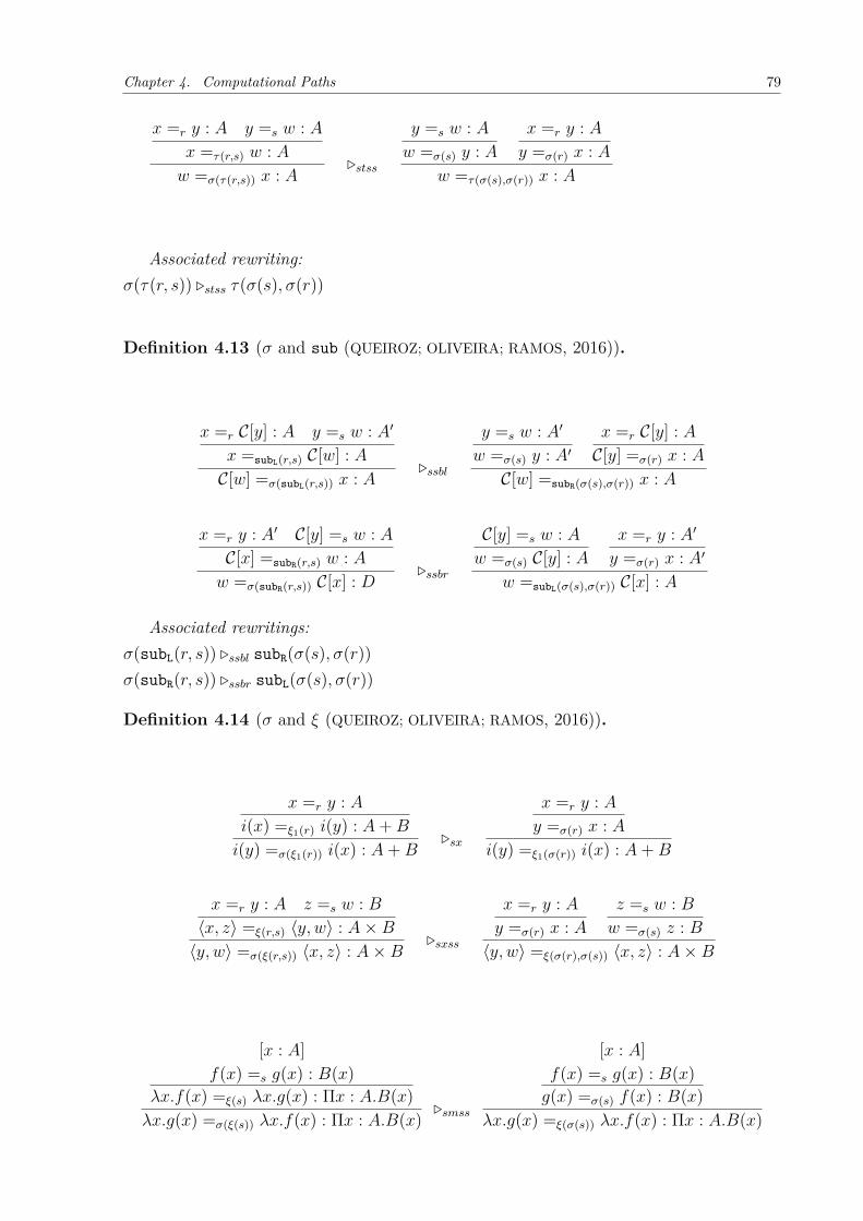
Chapter 4. Computational Paths 79
𝑥 =𝑟 𝑦 : 𝐴 𝑦 =𝑠 𝑤 : 𝐴𝑥 =𝜏(𝑟,𝑠) 𝑤 : 𝐴𝑤 =𝜎(𝜏(𝑟,𝑠)) 𝑥 : 𝐴 ◁𝑠𝑡𝑠𝑠
𝑦 =𝑠 𝑤 : 𝐴𝑤 =𝜎(𝑠) 𝑦 : 𝐴
𝑥 =𝑟 𝑦 : 𝐴𝑦 =𝜎(𝑟) 𝑥 : 𝐴
𝑤 =𝜏(𝜎(𝑠),𝜎(𝑟)) 𝑥 : 𝐴
Associated rewriting:𝜎(𝜏(𝑟, 𝑠)) ◁𝑠𝑡𝑠𝑠 𝜏(𝜎(𝑠), 𝜎(𝑟))
Definition 4.13 (𝜎 and sub (QUEIROZ; OLIVEIRA; RAMOS, 2016)).
𝑥 =𝑟 𝒞[𝑦] : 𝐴 𝑦 =𝑠 𝑤 : 𝐴′
𝑥 =subL(𝑟,𝑠) 𝒞[𝑤] : 𝐴𝒞[𝑤] =𝜎(subL(𝑟,𝑠)) 𝑥 : 𝐴 ◁𝑠𝑠𝑏𝑙
𝑦 =𝑠 𝑤 : 𝐴′
𝑤 =𝜎(𝑠) 𝑦 : 𝐴′𝑥 =𝑟 𝒞[𝑦] : 𝐴
𝒞[𝑦] =𝜎(𝑟) 𝑥 : 𝐴𝒞[𝑤] =subR(𝜎(𝑠),𝜎(𝑟)) 𝑥 : 𝐴
𝑥 =𝑟 𝑦 : 𝐴′ 𝒞[𝑦] =𝑠 𝑤 : 𝐴𝒞[𝑥] =subR(𝑟,𝑠) 𝑤 : 𝐴𝑤 =𝜎(subR(𝑟,𝑠)) 𝒞[𝑥] : 𝐷 ◁𝑠𝑠𝑏𝑟
𝒞[𝑦] =𝑠 𝑤 : 𝐴𝑤 =𝜎(𝑠) 𝒞[𝑦] : 𝐴
𝑥 =𝑟 𝑦 : 𝐴′
𝑦 =𝜎(𝑟) 𝑥 : 𝐴′
𝑤 =subL(𝜎(𝑠),𝜎(𝑟)) 𝒞[𝑥] : 𝐴
Associated rewritings:𝜎(subL(𝑟, 𝑠)) ◁𝑠𝑠𝑏𝑙 subR(𝜎(𝑠), 𝜎(𝑟))𝜎(subR(𝑟, 𝑠)) ◁𝑠𝑠𝑏𝑟 subL(𝜎(𝑠), 𝜎(𝑟))
Definition 4.14 (𝜎 and 𝜉 (QUEIROZ; OLIVEIRA; RAMOS, 2016)).
𝑥 =𝑟 𝑦 : 𝐴𝑖(𝑥) =𝜉1(𝑟) 𝑖(𝑦) : 𝐴+𝐵
𝑖(𝑦) =𝜎(𝜉1(𝑟)) 𝑖(𝑥) : 𝐴+𝐵◁𝑠𝑥
𝑥 =𝑟 𝑦 : 𝐴𝑦 =𝜎(𝑟) 𝑥 : 𝐴
𝑖(𝑦) =𝜉1(𝜎(𝑟)) 𝑖(𝑥) : 𝐴+𝐵
𝑥 =𝑟 𝑦 : 𝐴 𝑧 =𝑠 𝑤 : 𝐵⟨𝑥, 𝑧⟩ =𝜉(𝑟,𝑠) ⟨𝑦, 𝑤⟩ : 𝐴×𝐵
⟨𝑦, 𝑤⟩ =𝜎(𝜉(𝑟,𝑠)) ⟨𝑥, 𝑧⟩ : 𝐴×𝐵◁𝑠𝑥𝑠𝑠
𝑥 =𝑟 𝑦 : 𝐴𝑦 =𝜎(𝑟) 𝑥 : 𝐴
𝑧 =𝑠 𝑤 : 𝐵𝑤 =𝜎(𝑠) 𝑧 : 𝐵
⟨𝑦, 𝑤⟩ =𝜉(𝜎(𝑟),𝜎(𝑠)) ⟨𝑥, 𝑧⟩ : 𝐴×𝐵
[𝑥 : 𝐴]𝑓(𝑥) =𝑠 𝑔(𝑥) : 𝐵(𝑥)
𝜆𝑥.𝑓(𝑥) =𝜉(𝑠) 𝜆𝑥.𝑔(𝑥) : Π𝑥 : 𝐴.𝐵(𝑥)𝜆𝑥.𝑔(𝑥) =𝜎(𝜉(𝑠)) 𝜆𝑥.𝑓(𝑥) : Π𝑥 : 𝐴.𝐵(𝑥) ◁𝑠𝑚𝑠𝑠
[𝑥 : 𝐴]𝑓(𝑥) =𝑠 𝑔(𝑥) : 𝐵(𝑥)𝑔(𝑥) =𝜎(𝑠) 𝑓(𝑥) : 𝐵(𝑥)
𝜆𝑥.𝑔(𝑥) =𝜉(𝜎(𝑠)) 𝜆𝑥.𝑓(𝑥) : Π𝑥 : 𝐴.𝐵(𝑥)

Chapter 4. Computational Paths 80
Associated rewritings:𝜎(𝜉(𝑟)) ◁𝑠𝑥 𝜉(𝜎(𝑟))𝜎(𝜉(𝑟, 𝑠)) ◁𝑠𝑥𝑠𝑠 𝜉(𝜎(𝑟), 𝜎(𝑠))𝜎(𝜉(𝑠) ◁𝑠𝑚𝑠𝑠 𝜉(𝜎(𝑠))
Definition 4.15 (𝜎 and 𝜇 (QUEIROZ; OLIVEIRA; RAMOS, 2016)).
𝑥 =𝑟 𝑦 : 𝐴×𝐵
𝐹𝑆𝑇 (𝑥) =𝜇1(𝑟) 𝐹𝑆𝑇 (𝑦) : 𝐴𝐹𝑆𝑇 (𝑦) =𝜎(𝜇1(𝑟)) 𝐹𝑆𝑇 (𝑥) : 𝐴 ◁𝑠𝑚
𝑥 =𝑟 𝑦 : 𝐴×𝐵
𝑦 =𝜎(𝑟) 𝑥 : 𝐴×𝐵
𝐹𝑆𝑇 (𝑦) =𝜇1(𝜎(𝑟)) 𝐹𝑆𝑇 (𝑥) : 𝐴
𝑥 =𝑟 𝑦 : 𝐴×𝐵
𝑆𝑁𝐷(𝑥) =𝜇2(𝑟) 𝑆𝑁𝐷(𝑦) : 𝐴𝑆𝑁𝐷(𝑦) =𝜎(𝜇2(𝑟)) 𝑆𝑁𝐷(𝑥) : 𝐴 ◁𝑠𝑚
𝑥 =𝑟 𝑦 : 𝐴×𝐵
𝑦 =𝜎(𝑟) 𝑥 : 𝐴×𝐵
𝑆𝑁𝐷(𝑦) =𝜇2(𝜎(𝑟)) 𝑆𝑁𝐷(𝑥) : 𝐴
𝑥 =𝑠 𝑦 : 𝐴 𝑓 =𝑟 𝑔 : 𝐴 → 𝐵
𝐴𝑃𝑃 (𝑓, 𝑥) =𝜇(𝑠,𝑟) 𝐴𝑃𝑃 (𝑔, 𝑦) : 𝐵𝐴𝑃𝑃 (𝑔, 𝑦) =𝜎(𝜇(𝑠,𝑟)) 𝐴𝑃𝑃 (𝑓, 𝑥) : 𝐵
◁𝑠𝑚𝑠𝑠
𝑥 =𝑠 𝑦 : 𝐴𝑦 =𝜎(𝑠) 𝑥 : 𝐴
𝑓 =𝑟 𝑔 : 𝐴 → 𝐵
𝑔 =𝜎(𝑟) 𝑓 : 𝐴 → 𝐵
𝐴𝑃𝑃 (𝑔, 𝑦) =𝜇(𝜎(𝑠),𝜎(𝑟)) 𝐴𝑃𝑃 (𝑓, 𝑥) : 𝐵
𝑥 =𝑟 𝑦 : 𝐴+𝐵
[𝑠 : 𝐴]...
𝑑(𝑠) =𝑢 𝑓(𝑠) : 𝐶
[𝑡 : 𝐵]...
𝑒(𝑡) =𝑣 𝑔(𝑡) : 𝐶𝐷(𝑥, 𝑠𝑑(𝑠), 𝑡𝑒(𝑡)) =𝜇(𝑟,𝑢,𝑣) 𝐷(𝑦, 𝑠𝑓(𝑠), 𝑡𝑔(𝑡)) : 𝐶
𝐷(𝑦, 𝑠𝑓(𝑠), 𝑡𝑔(𝑡)) : 𝐶 =𝜎(𝜇(𝑟,𝑢,𝑣)) 𝐷(𝑥, 𝑠𝑑(𝑠), 𝑡𝑒(𝑡)) : 𝐶
◁𝑠𝑚𝑠𝑠𝑠
𝑥 =𝑟 𝑦 : 𝐴+𝐵𝑦 =𝜎(𝑟) 𝑥 : 𝐴+𝐵
[𝑠 : 𝐴]𝑑(𝑠) =𝑢 𝑓(𝑠) : 𝐶𝑓(𝑠) =𝜎(𝑢) 𝑑(𝑠) : 𝐶
[𝑡 : 𝐵]𝑒(𝑡) =𝑣 𝑔(𝑡) : 𝐶𝑔(𝑡) =𝜎(𝑣) 𝑒(𝑡) : 𝐶
𝐷(𝑦, 𝑠𝑓(𝑠), 𝑡𝑔(𝑡)) =𝜇(𝜎(𝑟),𝜎(𝑢),𝜎(𝑣)) 𝐷(𝑥, 𝑠𝑑(𝑠), 𝑡𝑒(𝑡)) : 𝐶
𝑒 =𝑠 𝑏 : Σ𝑥 : 𝐴.𝐵(𝑥)[𝑡 : 𝐴, 𝑔(𝑡) : 𝐵(𝑡)]𝑑(𝑔, 𝑡) =𝑟 𝑓(𝑔, 𝑡) : 𝐶
𝐸(𝑒, 𝑔𝑡𝑑(𝑔, 𝑡)) =𝜇(𝑠,𝑟) 𝐸(𝑏, 𝑔𝑡𝑓(𝑔, 𝑡)) : 𝐶𝐸(𝑏, 𝑔𝑡𝑓(𝑔, 𝑡)) =𝜎(𝜇(𝑠,𝑟)) 𝐸(𝑒, 𝑔𝑡𝑑(𝑔, 𝑡)) : 𝐶
◁𝑠𝑚𝑠𝑠
𝑒 =𝑠 𝑏 : Σ𝑥 : 𝐴.𝐵(𝑥)𝑏 =𝜎(𝑠) 𝑒 : Σ𝑥 : 𝐴.𝐵(𝑥)
[𝑡 : 𝐴, 𝑔(𝑡) : 𝐵(𝑡)]𝑑(𝑔, 𝑡) =𝑟 𝑓(𝑔, 𝑡) : 𝐶𝑓(𝑔, 𝑡) =𝜎(𝑟) 𝑑(𝑔, 𝑡) : 𝐶
𝐸(𝑏, 𝑔𝑡𝑓(𝑔, 𝑡)) =𝜇(𝜎(𝑠),𝜎(𝑟)) 𝐸(𝑒, 𝑔𝑡𝑑(𝑔, 𝑡)) : 𝐶
Associated rewritings:𝜎(𝜇1(𝑟)) ◁𝑠𝑚 𝜇1(𝜎(𝑟))

Chapter 4. Computational Paths 81
𝜎(𝜇2(𝑟)) ◁𝑠𝑚 𝜇2(𝜎(𝑟))𝜎(𝜇(𝑠, 𝑟)) ◁𝑠𝑚𝑠𝑠 𝜇(𝜎(𝑠), 𝜎(𝑟))𝜎(𝜇(𝑟, 𝑢, 𝑣)) ◁𝑠𝑚𝑠𝑠𝑠 𝜇(𝜎(𝑟), 𝜎(𝑢), 𝜎(𝑣))
Definition 4.16 (𝜏 and sub (QUEIROZ; OLIVEIRA; RAMOS, 2016)).
𝑥 =𝑟 𝒞[𝑦] : 𝐴 𝑦 =𝑠 𝑤 : 𝐴′
𝑥 =subL(𝑟,𝑠) 𝒞[𝑤] : 𝐴 𝒞[𝑤] =𝑡 𝑧 : 𝐴𝑥 =𝜏(subL(𝑟,𝑠),𝑡) 𝑧 : 𝐴
◁𝑡𝑠𝑏𝑙𝑙
𝑥 =𝑟 𝒞[𝑦] : 𝐴𝑦 =𝑠 𝑤 : 𝐴′ 𝒞[𝑤] =𝑡 𝑧 : 𝐴
𝒞[𝑦] =subR(𝑠,𝑡) 𝑧 : 𝐴𝑥 =𝜏(𝑟,subR(𝑠,𝑡)) 𝑧 : 𝐴
𝑦 =𝑠 𝑤 : 𝐴 𝒞[𝑤] =𝑡 𝑧 : 𝐴𝒞[𝑦] =subR(𝑠,𝑡) 𝑧 : 𝐴 𝑧 =𝑢 𝑣 : 𝐴
𝒞[𝑦] =𝜏(subR(𝑠,𝑡),𝑢) 𝑣 : 𝐴
◁𝑡𝑠𝑏𝑟𝑙
𝑦 =𝑠 𝑤 : 𝐷′𝒞[𝑤] =𝑡 𝑧 : 𝐴 𝑧 =𝑢 𝑣 : 𝐴
𝒞[𝑤] =𝜏(𝑡,𝑢) 𝑣 : 𝐴𝒞[𝑦] =subR(𝑠,𝜏(𝑡,𝑢)) 𝑣 : 𝐴
𝑥 =𝑟 𝒞[𝑧] : 𝐴𝒞[𝑧] =𝜌 𝒞[𝑧] : 𝐴 𝑧 =𝑠 𝑤 : 𝐴′
𝒞[𝑧] =subL(𝜌,𝑠) 𝒞[𝑤] : 𝐴𝑥 =𝜏(𝑟,subL(𝜌,𝑠)) 𝒞[𝑤] : 𝐴
◁𝑡𝑠𝑏𝑙𝑟𝑥 =𝑟 𝒞[𝑧] : 𝐴 𝑧 =𝑠 𝑤 : 𝐴′
𝑥 =subL(𝑟,𝑠) 𝒞[𝑤] : 𝐴
𝑥 =𝑟 𝒞[𝑤] : 𝐴𝑤 =𝑠 𝑧 : 𝐴′ 𝒞[𝑧] =𝜌 𝒞[𝑧] : 𝐴
𝒞[𝑤] =subR(𝑠,𝜌) 𝒞[𝑧] : 𝐴𝑥 =𝜏(𝑟,subR(𝑠,𝜌)) 𝒞[𝑧] : 𝐴
◁𝑡𝑠𝑏𝑟𝑟𝑥 =𝑟 𝒞[𝑤] : 𝐷 𝑤 =𝑠 𝑧 : 𝐴′
𝑥 =subL(𝑟,𝑠) 𝒞[𝑧] : 𝐴
Definition 4.17 (𝜏 and 𝜏 (QUEIROZ; OLIVEIRA; RAMOS, 2016)).
𝑥 =𝑡 𝑦 : 𝐴 𝑦 =𝑟 𝑤 : 𝐴𝑥 =𝜏(𝑡,𝑟) 𝑤 : 𝐴 𝑤 =𝑠 𝑧 : 𝐴
𝑥 =𝜏(𝜏(𝑡,𝑟),𝑠) 𝑧 : 𝐴
◁𝑡𝑡
𝑥 =𝑡 𝑦 : 𝐴𝑦 =𝑟 𝑤 : 𝐴 𝑤 =𝑠 𝑧 : 𝐴
𝑦 =𝜏(𝑟,𝑠) 𝑧 : 𝐴𝑥 =𝜏(𝑡,𝜏(𝑟,𝑠)) 𝑧 : 𝐴
Associated rewritings:𝜏(subL(𝑟, 𝑠), 𝑡) ◁𝑡𝑠𝑏𝑙𝑙 𝜏(𝑟, subR(𝑠, 𝑡))𝜏(subR(𝑠, 𝑡), 𝑢)) ◁𝑡𝑠𝑏𝑟𝑙 subR(𝑠, 𝜏(𝑡, 𝑢))

Chapter 4. Computational Paths 82
𝜏(𝑟, subL(𝜏, 𝑠)) ◁𝑡𝑠𝑏𝑙𝑟 subL(𝑟, 𝑠)𝜏(𝑟, subR(𝑠, 𝜏)) ◁𝑡𝑠𝑏𝑟𝑟 subL(𝑟, 𝑠)𝜏(𝜏(𝑡, 𝑟), 𝑠) ◁𝑡𝑡 𝜏(𝑡, 𝜏(𝑟, 𝑠))
Thus, we put together all those rules to compose our rewrite system:
Definition 4.18 (𝐿𝑁𝐷𝐸𝑄 − 𝑇𝑅𝑆 (QUEIROZ; OLIVEIRA; RAMOS, 2016)).1. 𝜎(𝜌) ◁𝑠𝑟 𝜌
2. 𝜎(𝜎(𝑟)) ◁𝑠𝑠 𝑟
3. 𝜏(𝒞[𝑟], 𝒞[𝜎(𝑟)]) ◁𝑡𝑟 𝒞[𝜌]4. 𝜏(𝒞[𝜎(𝑟)], 𝒞[𝑟]) ◁𝑡𝑠𝑟 𝒞[𝜌]5. 𝜏(𝒞[𝑟], 𝒞[𝜌]) ◁𝑡𝑟𝑟 𝒞[𝑟]6. 𝜏(𝒞[𝜌], 𝒞[𝑟]) ◁𝑡𝑙𝑟 𝒞[𝑟]7. subL(𝒞[𝑟], 𝒞[𝜌]) ◁𝑠𝑙𝑟 𝒞[𝑟]8. subR(𝒞[𝜌], 𝒞[𝑟]) ◁𝑠𝑟𝑟 𝒞[𝑟]9. subL(subL(𝑠, 𝒞[𝑟]), 𝒞[𝜎(𝑟)]) ◁𝑠𝑙𝑠 𝑠
10. subL(subL(𝑠, 𝒞[𝜎(𝑟)]), 𝒞[𝑟]) ◁𝑠𝑙𝑠𝑠 𝑠
11. subR(𝒞[𝑠], subR(𝒞[𝜎(𝑠)], 𝑟)) ◁𝑠𝑟𝑠 𝑟
12. subR(𝒞[𝜎(𝑠)], subR(𝒞[𝑠], 𝑟)) ◁𝑠𝑟𝑟𝑟 𝑟
13. 𝜇1(𝜉1(𝑟)) ◁𝑚𝑥2𝑙1 𝑟
14. 𝜇1(𝜉∧(𝑟, 𝑠)) ◁𝑚𝑥2𝑙2 𝑟
15. 𝜇2(𝜉∧(𝑟, 𝑠)) ◁𝑚𝑥2𝑟1 𝑠
16. 𝜇2(𝜉2(𝑠)) ◁𝑚𝑥2𝑟2 𝑠
17. 𝜇(𝜉1(𝑟), 𝑠, 𝑢) ◁𝑚𝑥3𝑙 𝑠
18. 𝜇(𝜉2(𝑟), 𝑠, 𝑢) ◁𝑚𝑥3𝑟 𝑢
19. 𝜈(𝜉(𝑟)) ◁𝑚𝑥𝑙 𝑟
20. 𝜇(𝜉2(𝑟), 𝑠) ◁𝑚𝑥𝑟 𝑠
21. 𝜉(𝜇1(𝑟), 𝜇2(𝑟)) ◁𝑚𝑥 𝑟
22. 𝜇(𝑡, 𝜉1(𝑟), 𝜉2(𝑠)) ◁𝑚𝑥𝑥 𝑡
23. 𝜉(𝜈(𝑟)) ◁𝑥𝑚𝑟 𝑟
24. 𝜇(𝑠, 𝜉2(𝑟)) ◁𝑚𝑥1𝑟 𝑠
25. 𝜎(𝜏(𝑟, 𝑠)) ◁𝑠𝑡𝑠𝑠 𝜏(𝜎(𝑠), 𝜎(𝑟))26. 𝜎(subL(𝑟, 𝑠)) ◁𝑠𝑠𝑏𝑙 subR(𝜎(𝑠), 𝜎(𝑟))27. 𝜎(subR(𝑟, 𝑠)) ◁𝑠𝑠𝑏𝑟 subL(𝜎(𝑠), 𝜎(𝑟))28. 𝜎(𝜉(𝑟)) ◁𝑠𝑥 𝜉(𝜎(𝑟))29. 𝜎(𝜉(𝑠, 𝑟)) ◁𝑠𝑥𝑠𝑠 𝜉(𝜎(𝑠), 𝜎(𝑟))30. 𝜎(𝜇(𝑟)) ◁𝑠𝑚 𝜇(𝜎(𝑟))31. 𝜎(𝜇(𝑠, 𝑟)) ◁𝑠𝑚𝑠𝑠 𝜇(𝜎(𝑠), 𝜎(𝑟))32. 𝜎(𝜇(𝑟, 𝑢, 𝑣)) ◁𝑠𝑚𝑠𝑠𝑠 𝜇(𝜎(𝑟), 𝜎(𝑢), 𝜎(𝑣))33. 𝜏(𝑟, subL(𝜌, 𝑠)) ◁𝑡𝑠𝑏𝑙𝑙 subL(𝑟, 𝑠)

Chapter 4. Computational Paths 83
34. 𝜏(𝑟, subR(𝑠, 𝜌)) ◁𝑡𝑠𝑏𝑟𝑙 subL(𝑟, 𝑠)35. 𝜏(subL(𝑟, 𝑠), 𝑡) ◁𝑡𝑠𝑏𝑙𝑟 𝜏(𝑟, subR(𝑠, 𝑡))36. 𝜏(subR(𝑠, 𝑡), 𝑢) ◁𝑡𝑠𝑏𝑟𝑟 subR(𝑠, 𝜏(𝑡, 𝑢))37. 𝜏(𝜏(𝑡, 𝑟), 𝑠) ◁𝑡𝑡 𝜏(𝑡, 𝜏(𝑟, 𝑠))38. 𝜏(𝒞[𝑢], 𝜏(𝒞[𝜎(𝑢)], 𝑣)) ◁𝑡𝑡𝑠 𝑣
39. 𝜏(𝒞[𝜎(𝑢)], 𝜏(𝒞[𝑢], 𝑣)) ◁𝑡𝑠𝑡 𝑢.
4.2.2 Normalization
In the previous subsection, we have seen a system of rewrite rules that resolves reductionsin a computational path. When we talk about these kind of systems, two questions arise:Every computational path has a normal form? And if a computational path has a normalform, is it unique? To show that it has a normal form, one has to prove that everycomputational path terminates, i.e., after a finite number of rewrites, one will end upwith a path that does not have any additional reduction. To show that it is unique, oneneeds to show that the system is confluent. In other words, if one has a path with 2 ormore reductions, one needs to show that the choice of the rewrite rule does not matter.In the end, one will always obtain the same end-path without any redundancies.
4.2.2.1 Termination
We are interested in the following theorem (QUEIROZ; OLIVEIRA; GABBAY, 2011; QUEIROZ;
OLIVEIRA; RAMOS, 2016):
Theorem 4.1 (Termination property for 𝐿𝑁𝐷𝐸𝑄−𝑇𝑅𝑆). 𝐿𝑁𝐷𝐸𝑄−𝑇𝑅𝑆 is terminating.
The proofs uses a special kind of ordering, known as recursive parth ordering, proposedby (DERSHOWITZ, 1982):
Definition 4.19 (Recursive path ordering (DERSHOWITZ, 1982; QUEIROZ; OLIVEIRA;
RAMOS, 2016)). Let > be a partial ordering on a set of operators F. The recursive pathordering >* on the set T(F) of terms over F is defined recursively as follows:
𝑠 = 𝑓(𝑠1, . . . , 𝑠𝑚) >* 𝑔(𝑡1, . . . , 𝑡𝑛) = 𝑡,
if and only if
1. 𝑓 = 𝑔 and {𝑠1, . . . , 𝑠𝑚} ≫* {𝑡1, . . . , 𝑡𝑛}, or
2. 𝑓 > 𝑔 and {𝑠} ≫* {𝑡1, . . . , 𝑡𝑛}, or
3. 𝑓 � 𝑔 and {𝑠1, . . . , 𝑠𝑚} ≫* or = {𝑡}
where ≫* is the extension of >* to multisets.

Chapter 4. Computational Paths 84
This definition uses the notion of partial ordering in multisets. A given partial ordering> on a set 𝑆 may be extended to a partial ordering ≫ on finite multisets of elements of𝑆, wherein a multiset is reduced by removing one or more elements and replacing themwith any finite number of elements, each oh which is smaller than one of the elementsremoved (DERSHOWITZ, 1982).
Thus, one can proof the termination property by showing that all rules 𝑒 → 𝑑 of thesystem, one has that 𝑒 >* 𝑑.
We also need to define the precedence ordering on the rewrite operators. We define asfollows (QUEIROZ; OLIVEIRA; RAMOS, 2016; QUEIROZ; OLIVEIRA; GABBAY, 2011):
𝜎 > 𝜏 > 𝜌,
𝜎 > 𝜉,
𝜎 > 𝜉∧,
𝜎 > 𝜉1,
𝜎 > 𝜉2,
𝜎 > 𝜇,
𝜎 > 𝜇1,
𝜎 > 𝜇2,
𝜎 > subL,
𝜎 > subR,
𝜏 > subL
Thus, one can prove the termination by showing that for every rule of 𝑒 → 𝑑 of𝐿𝑁𝐷𝐸𝑄 −𝑇𝑅𝑆, 𝑒 >* 𝑑. For almost every rule it is a straightforward and tedious process.We are not going to show those steps in this work. One can check the full proof in(QUEIROZ; OLIVEIRA; GABBAY, 2011).
4.2.2.2 Confluence
Before we go to the proof of confluence, one needs to notice that 𝐿𝑁𝐷𝐸𝑄−𝑇𝑅𝑆 is a condi-tional term rewriting system. This means that some rules can only be applied if the termsof the associated equation follow some rules. For example, for the rule 𝜇1(𝜉∧(𝑟, 𝑠))◁𝑚𝑥2𝑙2 𝑟,it is necessary to have an 𝛽-redex like 𝐹𝑆𝑇 ⟨𝑥, 𝑦⟩. With that in mind, one has the followingdefinition (QUEIROZ; OLIVEIRA; GABBAY, 2011):
Definition 4.20 (Conditional term rewriting system). In conditional term rewriting sys-tems, the rules have conditions attached, which must be true for the rewrite occur. Forexample, a rewrite rule 𝑒 → 𝑑 with condition 𝐶 is expressed as:
𝐶|𝑒 → 𝑑

Chapter 4. Computational Paths 85
To prove the confluence, one should analyze all possible critical pairs using the su-perposition algorithm proposed by (KNUTH; BENDIX, 1970). Thus, there should not beany divergent critical pair. For example, one can take the superposition of rules 1 and 2,obtaining: 𝜎(𝜎(𝜌)). We have two possible rewrites (QUEIROZ; OLIVEIRA; GABBAY, 2011):
• 𝜎(𝜎(𝜌)) B𝑠𝑟 𝜎(𝜌) B𝑠𝑟 𝜌
• 𝜎(𝜎(𝜌)) B𝑠𝑠 𝜌.
As one can see, we ended up with the same term 𝜌. Thus, no divergence has beengenerated.
One should compare every pair of rules to find all critical pairs and see if there are di-vergences. If some divergence happens, the superposition algorithm proposed by (KNUTH;
BENDIX, 1970) shows how to add new rules to the system in such a way that it be-comes confluent. As a matter of fact, that was the reason why the rules 38 and 39 of𝐿𝑁𝐷𝐸𝑄 −𝑇𝑅𝑆 have been introduced to the system (QUEIROZ; OLIVEIRA; RAMOS, 2016):
38. 𝜏(𝒞[𝑢], 𝜏(𝒞[𝜎(𝑢)], 𝑣)) ◁𝑡𝑡𝑠 𝑣
39. 𝜏(𝒞[𝜎(𝑢)], 𝜏(𝒞[𝑢], 𝑣)) ◁𝑡𝑠𝑡 𝑢.
Those two rules introduced the following reductions to the system (QUEIROZ; OLIVEIRA;
GABBAY, 2011):
𝑥 =𝑠 𝑢 : 𝐷
𝑥 =𝑠 𝑢 : 𝐷𝑢 =𝜎(𝑠) 𝑥 : 𝐷 𝑥 =𝑣 𝑤 : 𝐷
𝑢 =𝜏(𝜎(𝑠),𝑣) 𝑤 : 𝐷B𝑡𝑡𝑠 𝑥 =𝑣 𝑤
𝑥 =𝜏(𝑠,𝜏(𝜎(𝑠),𝑣)) 𝑤 : 𝐷
𝑥 =𝑠 𝑤 : 𝐷𝑤 =𝜎(𝑠) 𝑥 : 𝐷
𝑥 =𝑠 𝑤 : 𝐷 𝑤 =𝑣 𝑧 : 𝐷𝑥 =𝜏(𝑠,𝑣) 𝑧 : 𝐷
B𝑠𝑠 𝑤 =𝑣 𝑧𝑤 =𝜏(𝜎(𝑠),𝜏(𝑠,𝑣)) 𝑧 : 𝐷
One can check a full proof of confluence in (OLIVEIRA, 1995; OLIVEIRA; QUEIROZ,1994; OLIVEIRA; QUEIROZ, 1999; QUEIROZ; OLIVEIRA; GABBAY, 2011).
4.2.2.3 Normalization Procedure
We can now state two normalization theorems:
Theorem 4.2 (normalization (QUEIROZ; OLIVEIRA; GABBAY, 2011)). Every derivationin the 𝐿𝑁𝐷𝐸𝑄 − 𝑇𝑅𝑆 converts to a normal form.

Chapter 4. Computational Paths 86
Proof. Direct consequence of the termination property.
Theorem 4.3 (strong normalization (QUEIROZ; OLIVEIRA; GABBAY, 2011)). Every deriva-tion in the 𝐿𝑁𝐷𝐸𝑄 − 𝑇𝑅𝑆 converts to a unique normal form.
Proof. Direct consequence of the termination and confluence properties.
In this sense, every proof can be reduced to a normal one. To do that, one shouldidentify the redundancies and, based on the rewrite rules, one can construct a proofwithout any redundancies. We show that in an example. It is the following (QUEIROZ;
OLIVEIRA; GABBAY, 2011):
𝑓(𝑥, 𝑧) =𝑠 𝑓(𝑤, 𝑦) : 𝐷𝑓(𝑤, 𝑦) =𝜎(𝑠) 𝑓(𝑥, 𝑧) : 𝐷 𝑥 =𝑟 𝑐 : 𝐷
𝑓(𝑤, 𝑦) =𝑠𝑢𝑏𝐿(𝜎(𝑠),𝑟) 𝑓(𝑐, 𝑧) : 𝐷𝑓(𝑐, 𝑧) =𝜎(𝑠𝑢𝑏𝐿(𝜎(𝑠),𝑟)) 𝑓(𝑤, 𝑦) : 𝐷 𝑦 =𝑡 𝑏 : 𝐷
𝑓(𝑐, 𝑧) =𝑠𝑢𝑏𝐿(𝜎(𝑠𝑢𝑏𝐿(𝜎(𝑠),𝑟))) 𝑓(𝑤, 𝑏) : 𝐷
This deduction generates the following path: 𝑠𝑢𝑏𝐿(𝜎(𝑠𝑢𝑏𝐿(𝜎(𝑠), 𝑟))). This path is notin normal form, having two redundancies (QUEIROZ; OLIVEIRA; GABBAY, 2011):
𝑠𝑢𝑏𝐿(𝜎(𝑠𝑢𝑏𝐿(𝜎(𝑠), 𝑟))) B𝑠𝑠𝑏𝑙 𝑠𝑢𝑏𝐿(𝑠𝑢𝑏𝑅(𝜎(𝑟), 𝜎(𝜎(𝑠)), 𝑡)𝑠𝑢𝑏𝐿(𝑠𝑢𝑏𝑅(𝜎(𝑟), 𝜎(𝜎(𝑠)), 𝑡) B𝑠𝑠 𝑠𝑢𝑏𝐿(𝑠𝑢𝑏𝑅(𝜎(𝑟), 𝑠), 𝑡)
Thus, one can identify those reductions and conceive a deduction without any redun-dancies (QUEIROZ; OLIVEIRA; GABBAY, 2011):
𝑥 =𝑟 𝑐 : 𝐷𝑐 =𝜎(𝑟) 𝑥 : 𝐷 𝑓(𝑥, 𝑧) =𝑠 𝑓(𝑤, 𝑦) : 𝐷
𝑓(𝑐, 𝑧) =𝑠𝑢𝑏𝑅(𝜎(𝑟),𝑠) 𝑓(𝑤, 𝑦) : 𝐷 𝑦 =𝑡 𝑏 : 𝐷𝑓(𝑐, 𝑧) =𝑠𝑢𝑏𝐿(𝑠𝑢𝑏𝑅(𝜎(𝑟),𝑠),𝑡) 𝑓(𝑤, 𝑏) : 𝐷
4.2.3 Rewrite Equality
As we have just seen, the 𝐿𝑁𝐷𝐸𝑄 − 𝑇𝑅𝑆 has 39 rewrite rules. We call each rule as arewrite rule (abbreviation: rw-rule). We have the following definition:
Definition 4.21 (Rewrite Rule (RAMOS; QUEIROZ; OLIVEIRA, 2017)). An 𝑟𝑤-rule is anyof the rules defined in 𝐿𝑁𝐷𝐸𝑄 − 𝑇𝑅𝑆.
Similarly to the 𝛽-reduction of 𝜆-calculus, we have a definition for rewrite reduction:

Chapter 4. Computational Paths 87
Definition 4.22 (Rewrite reduction (RAMOS; QUEIROZ; OLIVEIRA, 2017)). Let 𝑠 and 𝑡 becomputational paths. We say that 𝑠B1𝑟𝑤 𝑡 (read as: 𝑠 𝑟𝑤-contracts to 𝑡) iff we can obtain𝑡 from 𝑠 by an application of only one 𝑟𝑤-rule. If 𝑠 can be reduced to 𝑡 by finite numberof 𝑟𝑤-contractions, then we say that 𝑠B𝑟𝑤 𝑡 (read as 𝑠 𝑟𝑤-reduces to 𝑡).
We also have rewrite contractions and equality:
Definition 4.23 (Rewrite contraction and equality (RAMOS; QUEIROZ; OLIVEIRA, 2017)).Let 𝑠 and 𝑡 be computational paths. We say that 𝑠 =𝑟𝑤 𝑡 (read as: 𝑠 is 𝑟𝑤-equal to 𝑡) iff 𝑡
can be obtained from 𝑠 by a finite (perhaps empty) series of 𝑟𝑤-contractions and reversed𝑟𝑤-contractions. In other words, 𝑠 =𝑟𝑤 𝑡 iff there exists a sequence 𝑅0, ...., 𝑅𝑛, with 𝑛 ≥ 0,such that
(∀𝑖 ≤ 𝑛− 1)(𝑅𝑖 B1𝑟𝑤 𝑅𝑖+1 or 𝑅𝑖+1 B1𝑟𝑤 𝑅𝑖)𝑅0 ≡ 𝑠, 𝑅𝑛 ≡ 𝑡
A fundamental result is the fact that rewrite equality is an equivalence relation(RAMOS; QUEIROZ; OLIVEIRA, 2017):
Proposition 4.1. Rewrite equality is transitive, symmetric and reflexive.
Proof. Comes directly from the fact that 𝑟𝑤-equality is the transitive, reflexive and sym-metric closure of 𝑟𝑤.
Rewrite reduction and equality play fundamental roles in the groupoid model of a typebased on computational paths, as we are going to see in the sequel.
4.2.4 𝐿𝑁𝐷𝐸𝑄 − 𝑇𝑅𝑆2
Until now, this subsection has concluded that there exist redundancies which are resolvedby a system called 𝐿𝑁𝐷𝐸𝑄 − 𝑇𝑅𝑆. This system establishes rules that reduces theseredundancies. Moreover, we concluded that these redundancies are just redundant usesof the equality axioms showed in section 2. In fact, since these axioms just define anequality theory for type theory, one can specify and say that these are redundancies ofthe equality of type theory. As we mentioned, the 𝐿𝑁𝐷𝐸𝑄 − 𝑇𝑅𝑆 has a total of 39rules(OLIVEIRA, 1995; QUEIROZ; OLIVEIRA; RAMOS, 2016). Since the 𝑟𝑤-equality is basedon the rules of 𝐿𝑁𝐷𝐸𝑄 − 𝑇𝑅𝑆, one can just imagine the high number of redundanciesthat 𝑟𝑤-equality could cause. In fact, a thoroughly study of all the redundancies causedby these rules could generate an entire new work. Fortunately, we are only interested inthe redundancies caused by the fact that 𝑟𝑤-equality is transitive, reflexive and symmetricwith the addition of only one specific 𝑟𝑤2-rule. Let’s say that we have a system, called𝐿𝑁𝐷𝐸𝑄 −𝑇𝑅𝑆2, that resolves all the redundancies caused by 𝑟𝑤-equality (the same waythat 𝐿𝑁𝐷𝐸𝑄−𝑇𝑅𝑆 resolves all the redundancies caused by equality). Since we know that𝑟𝑤-equality is transitive, symmetric and reflexive, it should have the same redundancies
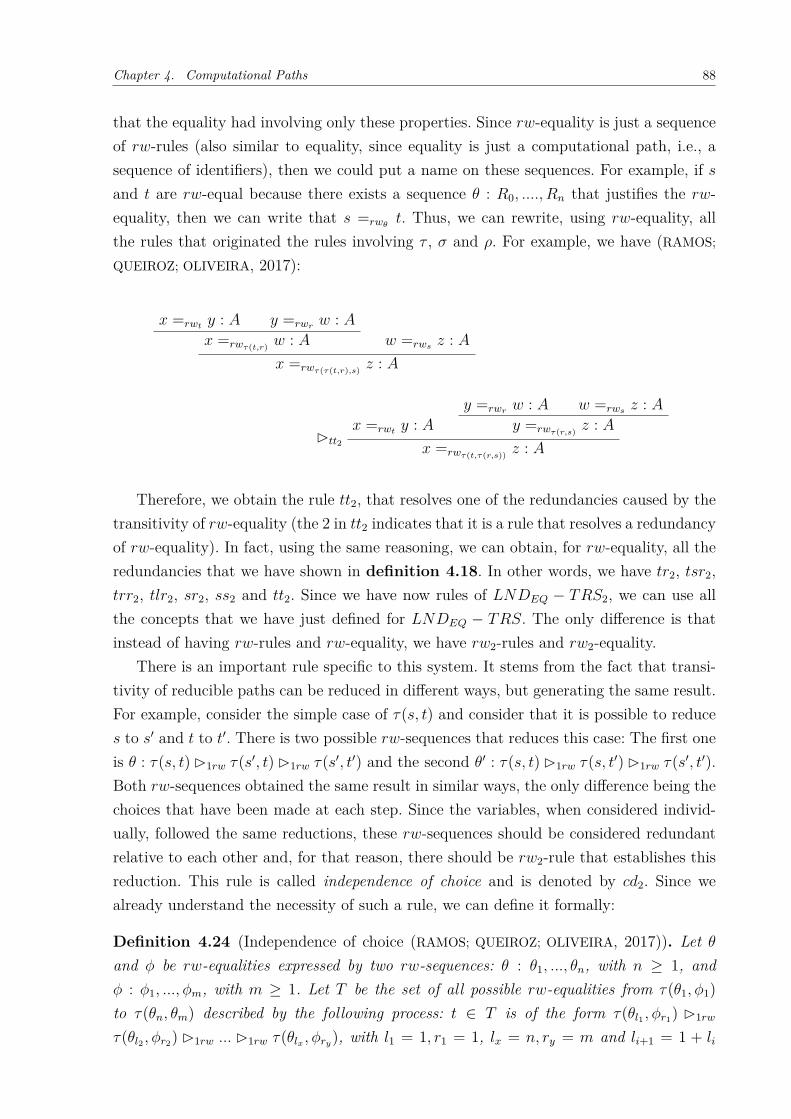
Chapter 4. Computational Paths 88
that the equality had involving only these properties. Since 𝑟𝑤-equality is just a sequenceof 𝑟𝑤-rules (also similar to equality, since equality is just a computational path, i.e., asequence of identifiers), then we could put a name on these sequences. For example, if 𝑠and 𝑡 are 𝑟𝑤-equal because there exists a sequence 𝜃 : 𝑅0, ...., 𝑅𝑛 that justifies the 𝑟𝑤-equality, then we can write that 𝑠 =𝑟𝑤𝜃
𝑡. Thus, we can rewrite, using 𝑟𝑤-equality, allthe rules that originated the rules involving 𝜏 , 𝜎 and 𝜌. For example, we have (RAMOS;
QUEIROZ; OLIVEIRA, 2017):
𝑥 =𝑟𝑤𝑡 𝑦 : 𝐴 𝑦 =𝑟𝑤𝑟 𝑤 : 𝐴𝑥 =𝑟𝑤𝜏(𝑡,𝑟) 𝑤 : 𝐴 𝑤 =𝑟𝑤𝑠 𝑧 : 𝐴
𝑥 =𝑟𝑤𝜏(𝜏(𝑡,𝑟),𝑠) 𝑧 : 𝐴
𝑥 =𝑟𝑤𝑡 𝑦 : 𝐴𝑦 =𝑟𝑤𝑟 𝑤 : 𝐴 𝑤 =𝑟𝑤𝑠 𝑧 : 𝐴
𝑦 =𝑟𝑤𝜏(𝑟,𝑠) 𝑧 : 𝐴B𝑡𝑡2 𝑥 =𝑟𝑤𝜏(𝑡,𝜏(𝑟,𝑠)) 𝑧 : 𝐴
Therefore, we obtain the rule 𝑡𝑡2, that resolves one of the redundancies caused by thetransitivity of 𝑟𝑤-equality (the 2 in 𝑡𝑡2 indicates that it is a rule that resolves a redundancyof 𝑟𝑤-equality). In fact, using the same reasoning, we can obtain, for 𝑟𝑤-equality, all theredundancies that we have shown in definition 4.18. In other words, we have 𝑡𝑟2, 𝑡𝑠𝑟2,𝑡𝑟𝑟2, 𝑡𝑙𝑟2, 𝑠𝑟2, 𝑠𝑠2 and 𝑡𝑡2. Since we have now rules of 𝐿𝑁𝐷𝐸𝑄 − 𝑇𝑅𝑆2, we can use allthe concepts that we have just defined for 𝐿𝑁𝐷𝐸𝑄 − 𝑇𝑅𝑆. The only difference is thatinstead of having 𝑟𝑤-rules and 𝑟𝑤-equality, we have 𝑟𝑤2-rules and 𝑟𝑤2-equality.
There is an important rule specific to this system. It stems from the fact that transi-tivity of reducible paths can be reduced in different ways, but generating the same result.For example, consider the simple case of 𝜏(𝑠, 𝑡) and consider that it is possible to reduce𝑠 to 𝑠′ and 𝑡 to 𝑡′. There is two possible 𝑟𝑤-sequences that reduces this case: The first oneis 𝜃 : 𝜏(𝑠, 𝑡) B1𝑟𝑤 𝜏(𝑠′, 𝑡) B1𝑟𝑤 𝜏(𝑠′, 𝑡′) and the second 𝜃′ : 𝜏(𝑠, 𝑡) B1𝑟𝑤 𝜏(𝑠, 𝑡′) B1𝑟𝑤 𝜏(𝑠′, 𝑡′).Both 𝑟𝑤-sequences obtained the same result in similar ways, the only difference being thechoices that have been made at each step. Since the variables, when considered individ-ually, followed the same reductions, these 𝑟𝑤-sequences should be considered redundantrelative to each other and, for that reason, there should be 𝑟𝑤2-rule that establishes thisreduction. This rule is called independence of choice and is denoted by 𝑐𝑑2. Since wealready understand the necessity of such a rule, we can define it formally:
Definition 4.24 (Independence of choice (RAMOS; QUEIROZ; OLIVEIRA, 2017)). Let 𝜃and 𝜑 be 𝑟𝑤-equalities expressed by two 𝑟𝑤-sequences: 𝜃 : 𝜃1, ..., 𝜃𝑛, with 𝑛 ≥ 1, and𝜑 : 𝜑1, ..., 𝜑𝑚, with 𝑚 ≥ 1. Let 𝑇 be the set of all possible 𝑟𝑤-equalities from 𝜏(𝜃1, 𝜑1)to 𝜏(𝜃𝑛, 𝜃𝑚) described by the following process: 𝑡 ∈ 𝑇 is of the form 𝜏(𝜃𝑙1 , 𝜑𝑟1) B1𝑟𝑤
𝜏(𝜃𝑙2 , 𝜑𝑟2) B1𝑟𝑤 ... B1𝑟𝑤 𝜏(𝜃𝑙𝑥 , 𝜑𝑟𝑦), with 𝑙1 = 1, 𝑟1 = 1, 𝑙𝑥 = 𝑛, 𝑟𝑦 = 𝑚 and 𝑙𝑖+1 = 1 + 𝑙𝑖

Chapter 4. Computational Paths 89
and 𝑟𝑖+1 = 𝑟𝑖 or 𝑙𝑖+1 = 𝑙𝑖 and 𝑟𝑖+1 = 1 + 𝑟𝑖. The independence of choice, denoted by 𝑐𝑑2,is defined as the rule of 𝐿𝑁𝐷𝐸𝑄 − 𝑇𝑅𝑆2 that establishes the equality between any twodifferent terms of 𝑇 . In other words, if 𝑥, 𝑦 ∈ 𝑇 and 𝑥 ̸= 𝑦, then 𝑥 =𝑐𝑑2 𝑦 and 𝑦 =𝑐𝑑2 𝑥.
Analogously to the 𝑟𝑤-equality, 𝑟𝑤2-equality is also an equivalence relation (RAMOS;
QUEIROZ; OLIVEIRA, 2017):
Proposition 4.2. 𝑟𝑤2-equality is transitive, symmetric and reflexive.
Proof. Analogous to Proposition 4.1.
4.3 GROUPOID MODEL
In this section, we use categorical concepts introduced in the previous chapter to show thatwe can use computational paths to induce a groupoid structure of a type. Nevertheless,before we do that, we show that computational paths form a globular structure.
4.3.1 Globular Structure
In the previous section, we have just shown the existence of paths between computationalpaths. Such paths were originated from redundancies caused by 𝑟𝑤-equality. Analogously,one could think of redundancies caused by 𝑟𝑤2-equality, which would be resolved by theestablishment of computational paths between two equivalent 𝑟𝑤2-equalities. With thatin mind, we can extend this process up to the infinity. That way, we obtain an infinitenumber of 𝑟𝑤𝑛-equalities and 𝐿𝑁𝐷𝐸𝑄 − 𝑇𝑅𝑆𝑛 systems. We have seen in the previouschapter a mathematical entity suitable to express this fact. It is known as globular set.With that in mind, we have the following definition:
Definition 4.25 (Level of a path (RAMOS; QUEIROZ; OLIVEIRA, 2017)). The 𝑙𝑒𝑣𝑒𝑙 of apath is defined as follows:
• If 𝑎, 𝑏 : 𝐴 are terms such that 𝑎 and 𝑏 are not 𝑟𝑤-equalities, then we say that a path𝑎 =𝑠 𝑏 has level 1.
• If 𝑟, 𝑠 : 𝐴 are 𝑟𝑤𝑛-equalities, then a path 𝑟 =𝜃 𝑠 has level 𝑛+ 1.
The idea is that if we have two 𝑛-level paths 𝑟 and 𝑠 and if 𝑟 can be rewritten into 𝑠by a sequence of rewrites established by 𝐿𝑁𝐷𝐸𝑄 − 𝑇𝑅𝑆𝑛, then this sequence of rewritesis a (𝑛+ 1)-level path that establishes 𝑟 =𝑟𝑤𝑛 𝑠.
Computational paths can form a globular-set structure. To see this, consider 𝑋(𝑛)as the set of 𝑛-level paths between two (𝑛 − 1)-level paths (for 𝑛 = 0, just consider twonon-path objects) and for any path 𝑥 =𝑚 𝑦, consider that 𝑠(𝑚) = 𝑥 and 𝑡(𝑚) = 𝑦. Thatway, if 𝑛 ≥ 2 and 𝑚 ∈ 𝑋(𝑛), then 𝑠(𝑚) ∈ 𝑋(𝑛 − 1) and 𝑡(𝑚) ∈ 𝑋(𝑛 − 1). Now, if we

Chapter 4. Computational Paths 90
consider two 𝑛-level paths 𝑡 =𝜃 𝑚, and 𝑡 =𝛼 𝑚 and a (𝑛 + 1)-level path 𝜃 =𝜑 𝛼, thefollowing equations hold (RAMOS; QUEIROZ; OLIVEIRA, 2017):
𝑠(𝑠(𝜑)) = 𝑠(𝜃) = 𝑡 = 𝑠(𝛼) = 𝑠(𝑡(𝜑)).𝑡(𝑠(𝜑)) = 𝑡(𝜃) = 𝑚 = 𝑡(𝛼) = 𝑡(𝑡(𝜑)).
All globular-set conditions hold. Then, we can think that computational paths form aglobular set structure all up to infinity, i.e., a ∞-globular-set.
4.3.2 The Induced Groupoid
The relation between the algebraic structure of groupoid and the identity type was firstnoticed by(HOFMANN; STREICHER, 1994). In this work, the authors claim that it is pos-sible to think of any type of type theory as having a groupoid structure. To do that, onecould think of the terms of a type as objects and the propositional identities betweenthese terms to be morphisms. Using 𝐽 ,(HOFMANN; STREICHER, 1994) showed that thefollowing types, which correspond to the groupoid equations, are inhabited:
• 𝐼𝑑𝐼𝑑𝐴(𝑥,𝑧)(𝑡𝑟𝑎𝑛𝑠(𝑡𝑟𝑎𝑛𝑠(𝑝, 𝑞), 𝑟), 𝑡𝑟𝑎𝑛𝑠(𝑝, 𝑡𝑟𝑎𝑛𝑠(𝑞, 𝑟)))
• 𝐼𝑑𝐼𝑑𝐴(𝑥,𝑦)(𝑡𝑟𝑎𝑛𝑠(𝑟𝑒𝑓𝑙(𝑥), 𝑟), 𝑟)
• 𝐼𝑑𝐼𝑑𝐴(𝑥,𝑦)(𝑡𝑟𝑎𝑛𝑠(𝑟, 𝑟𝑒𝑓𝑙(𝑥)), 𝑟)
• 𝐼𝑑𝐼𝑑𝐴(𝑦,𝑦)(𝑡𝑟𝑎𝑛𝑠(𝑠𝑦𝑚𝑚(𝑟), 𝑟), 𝑟𝑒𝑓𝑙(𝑥))
• 𝐼𝑑𝐼𝑑𝐴(𝑥,𝑥)(𝑡𝑟𝑎𝑛𝑠(𝑟, 𝑠𝑦𝑚𝑚(𝑟)), 𝑟𝑒𝑓𝑙(𝑥))
• 𝐼𝑑𝐼𝑑𝐴(𝑥,𝑦)(𝑠𝑦𝑚𝑚(𝑠𝑦𝑚𝑚(𝑟)), 𝑟)
After this important work, the authors further develop their ideas in (HOFMANN;
STREICHER, 1998), showing how 𝐽 can be interpreted categorically.Since our approach is not based on 𝐽 , but on the fact that identities are established by
computational paths, our objective in this section is to show that computational paths,together with the reduction rules discussed in the last section, are also capable of inducinggroupoidal structures.
Before we conclude that computational paths induces categories with groupoid prop-erties, we need to make clear the difference between a strict and a weak category. As onewill see, the word weak will appear many times. This will be the case because some ofthe categorical equalities will not hold “on the nose", so to say. They will hold up to 𝑟𝑤-equality or up to higher levels of 𝑟𝑤-equalities. This is similar to the groupoid model ofthe identity type proposed by(HOFMANN; STREICHER, 1994). In (HOFMANN; STREICHER,1994), the equalities do not hold “on the nose ", they hold up to propositional equality (orup to homotopy if one uses the homotopy interpretation). To indicate that these equalities

Chapter 4. Computational Paths 91
hold only up to some property, we say that the induced structure is a weak categoricalstructure. This will be even more clear in the proof of the following proposition (RAMOS;
QUEIROZ; OLIVEIRA, 2017):
Proposition 4.3. For each type 𝐴, computational paths induces a weak categorical struc-ture called 𝐴𝑟𝑤.
Proof. Since we are working with categories, a good understanding of the basic conceptof what is a category is essential. If one is not familiarized with the concept, one shouldcheck the chapter 3 of this work. To sum up, a category is a structure with objectsand morphisms between these objects. These morphisms must obey two main laws: theassociative and identity laws. To define a weak categorical structure 𝐴𝑟𝑤, the first step isto define the objects, the morphisms:
• Objects: The objects of 𝐴𝑟𝑤 are terms 𝑎 of the type 𝐴, i.e., 𝑎 : 𝐴.
• Morphisms: A morphism (arrow) between terms 𝑎 : 𝐴 and 𝑏 : 𝐴 are arrows 𝑠 : 𝑎 → 𝑏
such that 𝑠 is a computational path between the terms, i.e., 𝑎 =𝑠 𝑏 : 𝐴.
We need now to define the composition of morphisms, the identity morphism and checkthe associative and identity laws. Since we are working in a weak context, the associativeand identity law needs only to hold up to 𝑟𝑤-equality. Before we check all these conditions,we can represent this structure in the following diagram:
𝑎 : 𝐴 𝑏 : 𝐴
𝑐 : 𝐴 𝑑 : 𝐴
𝜌𝑎𝑠
𝜏(𝑠,𝑟)
𝜌𝑏
𝑟𝜏(𝑟,𝑡)
𝜌𝑐
𝑡 𝜌𝑑
• Compositions: Given arrows (paths) 𝑠 : 𝑎 → 𝑏 and 𝑟 : 𝑏 → 𝑐, we need to find anarrow 𝑡 : 𝑎 → 𝑐 such that 𝑡 = 𝑟 ∘ 𝑠. To do that, we first need to define the meaningof a composition of paths. Since equality has the transitive axiom, it is natural todefine the composition as an application of the transitivity, i.e. 𝑡 = 𝑟 ∘ 𝑠 = 𝜏(𝑠, 𝑟).Therefore, for any 𝑠 : 𝑎 → 𝑏 and 𝑟 : 𝑏 → 𝑐, we always have a 𝑡 = 𝑟 ∘ 𝑠 = 𝜏(𝑠, 𝑟).
• Associativity of the composition: Given arrows 𝑠 : 𝑎 → 𝑏, 𝑟 : 𝑏 → 𝑐 and 𝑡 : 𝑐 →𝑑, since we are working with a weak categorical structure, we need to concludethat 𝑡 ∘ (𝑟 ∘ 𝑠) =𝑟𝑤 (𝑡 ∘ 𝑟) ∘ 𝑠. Substituting the compositions by the correspondingtransitivities, we need to conclude that 𝜏(𝜏(𝑠, 𝑟), 𝑡) =𝑟𝑤 𝜏(𝑠, 𝜏(𝑟, 𝑡)). This is a direct

Chapter 4. Computational Paths 92
consequence of the rule 𝑡𝑡: 𝜏(𝜏(𝑠, 𝑟), 𝑡) B𝑡𝑡 𝜏(𝑠, 𝜏(𝑟, 𝑡)). Therefore, we conclude that𝜏(𝜏(𝑠, 𝑟), 𝑡) =𝑟𝑤 𝜏(𝑠, 𝜏(𝑟, 𝑡)).
• Identity morphism: For any object 𝑎, consider the reflexive path 𝑎 =𝜌 𝑎 as theidentity arrow 1𝑎. Let’s call this path as 𝜌𝑎 (to indicate that it is a reflexive path of𝑎).
• Identity law: For any arrows (paths) 𝑠 : 𝑎 → 𝑏, we need to show that 𝑠 ∘ 1𝑎 = 𝑠 =1𝑏 ∘ 𝑠. This can be shown (also in a weak sense) with a straightforward applicationof 𝑟𝑤-rules. We have that 𝑠 ∘ 1𝑎 = 𝑠 ∘ 𝜌𝑎 = 𝜏(𝜌𝑎, 𝑠) B𝑡𝑙𝑟 𝑠, therefore 𝜏(𝜌𝑎, 𝑠) =𝑟𝑤 𝑠.For the other equation, we have that 1𝑏 ∘ 𝑠 = 𝜌𝑏 ∘ 𝑠 = 𝜏(𝑠, 𝜌𝑏) B𝑡𝑟𝑟 𝑠 and thus,𝜏(𝑠, 𝜌𝑏) =𝑟𝑤 𝑠.
Since all these conditions have been satisfied, we conclude that the structure 𝐴𝑟𝑤 inducedby computational paths is a weak categorical structure.
Is it possible to induce a strict (i.e., one that the equalities will hold “on the nose ")using computational paths? The answer is yes. Since 𝑟𝑤-equality is transitive, symmetricand reflexive, 𝑟𝑤-equality is an equivalence relation. If we use equivalent classes of 𝑟𝑤-equalities as arrows, the equalities will hold “on the nose ". Since we are trying to provesimilar results to the ones obtained for identity types by(HOFMANN; STREICHER, 1994) (in(HOFMANN; STREICHER, 1994), as mentioned before, the equalities only in a weak sense),we are more interested in this weak categorical structure that we have just obtained.
We can now show that 𝐴𝑟𝑤 has a groupoid structure (RAMOS; QUEIROZ; OLIVEIRA,2017):
Proposition 4.4. The induced structure 𝐴𝑟𝑤 has a weak groupoidal structure.
Proof. We need to show that every arrow is an isomorphism. Since we are working ina weak sense, the isomorphism equalities need only to hold up to 𝑟𝑤-equality. To showthat, for every arrow 𝑠 : 𝑎 → 𝑏, we need to show a 𝑡 : 𝑏 → 𝑎 such that 𝑡 ∘ 𝑠 =𝑟𝑤 1𝑎 and𝑠 ∘ 𝑡 =𝑟𝑤 1𝑏. To do that, recall that every computational path has an inverse path 𝜎(𝑠).Put 𝑡 = 𝜎(𝑠). Thus, we have that 𝑠 ∘ 𝑡 = 𝑠 ∘ 𝜎(𝑠) = 𝜏(𝜎(𝑠), 𝑠) B𝑡𝑠𝑟 𝜌𝑏. Since 𝜌𝑏 = 1𝑏, weconclude that 𝑠∘ 𝑡 =𝑟𝑤 1𝑏. We also have that 𝑡∘𝑠 = 𝜎(𝑠)∘𝑠 = 𝜏(𝑠, 𝜎(𝑠))B𝑡𝑟 𝜌𝑎. Therefore,𝑡 ∘ 𝑠 = 1𝑎. We conclude that every arrow is a weak isomorphism and thus, 𝐴𝑟𝑤 is a weakgroupoidal structure.
If we work with classes of equivalences as arrows, we can obtain a groupoidal struc-ture in the strict sense. With that, we finally conclude that computational paths have agroupoid model. As one could notice, we only needed to use the properties of computa-tional paths, together with rules of the rewrites 𝐿𝑁𝐷𝐸𝑄 − 𝑇𝑅𝑆. Having these conceptsand rules, we have just needed to show that computational paths induces simple structures

Chapter 4. Computational Paths 93
of category theory. The groupoidal model came naturally from the concept of computa-tional paths, without the need of constructing any complex term of an identity type, asdone in (HOFMANN; STREICHER, 1994). The fact that computational paths have a naturalgroupoidal model is an advantage, since it will automatically imply that the identity typehas a natural groupoidal model (without needing to build any term using a constructor,like the constructor 𝐽 of the traditional identity type).
4.3.3 Higher Structures
We have just shown that computational paths induce a weak groupoidal structure knownas 𝐴𝑟𝑤. We also know that the arrows (or morphisms) of 𝐴𝑟𝑤 are computational pathsbetween two terms of a type 𝐴. As we saw in the previous subsection, sometimes acomputational path can be reduced to another by rules that we called 𝑟𝑤-rules. That way,if we have terms 𝑎, 𝑏 : 𝐴 and paths between these terms, we can define a new structure.This new structure, called 𝐴2𝑟𝑤(𝑎, 𝑏), has objects as computational paths between 𝑎 and𝑏 and there is a morphism between paths 𝑎 =𝑠 𝑏 and 𝑎 =𝑡 𝑏 iff 𝑠 =𝑟𝑤 𝑡. Since 𝑟𝑤-equalityis transitive, reflexive and symmetric, 𝐴2𝑟𝑤 is a weak categorical structure which theequalities hold up to 𝑟𝑤2-equality. The proof of this fact is analogous to the proposition4.1. The sole difference is the fact that since the morphisms are 𝑟𝑤-equalities, insteadof computational paths, all the equalities will hold up to 𝑟𝑤2-equality. To see this, takethe example of the associativity. Looking at the 𝐿𝑁𝐷𝐸𝑄 − 𝑇𝑅𝑆2 system, we have that𝜏(𝜏(𝜃, 𝜎), 𝜑) B𝑡𝑡2 𝜏(𝜃, 𝜏(𝜎, 𝜑)) (𝜃, 𝜎 and 𝜑 represent 𝑟𝑤-equalities between paths from 𝑎
to 𝑏). Therefore, 𝜏(𝜏(𝜃, 𝜎), 𝜑) =𝑟𝑤2 𝜏(𝜃, 𝜏(𝜎, 𝜑)). The associative law holds up to 𝑟𝑤2-equality. As one can easily check, the identity law will also hold up to 𝑟𝑤2-equality.Therefore, 𝐴2𝑟𝑤(𝑎, 𝑏) has a weak categorical structure. Analogous to proposition 4.4, thegroupoid law will also hold up to 𝑟𝑤2-equality.
Instead of considering 𝐴𝑟𝑤 and 𝐴2𝑟𝑤(𝑎, 𝑏) as separated structures, we can think of aunique structure with 2-levels. The first level is 𝐴𝑟𝑤 and the second one is the structure𝐴2𝑟𝑤(𝑎, 𝑏) between each pair of objects 𝑎, 𝑏 ∈ 𝐴𝑟𝑤. We call this structure 2 − 𝐴𝑟𝑤. Themorphisms of the first level are called 1-morphisms and the ones of the second level arecalled 2-morphisms (also known as 2-arrows or 2-cells). Since it has multiple levels, itis considered a higher structure. We want to prove that this structure is a categoricalstructure known as weak 2-category. The main problem is the fact that in a weak 2-category, the last level (i.e., the second level) needs to hold up in a strict sense. This isnot the case for 2−𝐴2𝑟𝑤, since each 𝐴2𝑟𝑤(𝑎, 𝑏) only holds up to 𝑟𝑤2-equality. Nevertheless,there still a way to induce this weak 2-category. Since 𝑟𝑤-equality is an equivalence relation(because it is transitive, symmetric and reflexive), we can consider a special 𝐴2𝑟𝑤(𝑎, 𝑏),where the arrows are the arrows of 𝐴2𝑟𝑤(𝑎, 𝑏) modulo 𝑟𝑤2-equality. That way, since theequalities hold up to 𝑟𝑤2-equality in 𝐴2𝑟𝑤(𝑎, 𝑏), they will hold in a strict sense when weconsider the equivalence classes of 𝑟𝑤2-equality. We call this structure [𝐴2𝑟𝑤(𝑎, 𝑏)]. In this

Chapter 4. Computational Paths 94
structure, consider the composition of arrows defined as: [𝜃]𝑟𝑤2 ∘ [𝜑]𝑟𝑤2 = [𝜃 ∘ 𝜑]𝑟𝑤2 . Now,we can think of the structure [2−𝐴𝑟𝑤]. This structure is similar to 2−𝐴𝑟𝑤. The differenceis that the categories of the second level are [𝐴2𝑟𝑤(𝑎, 𝑏)] instead of 𝐴2𝑟𝑤(𝑎, 𝑏). We can nowprove that [2 − 𝐴𝑟𝑤] is a weak 2-category (RAMOS; QUEIROZ; OLIVEIRA, 2017):
Proposition 4.5. Computational paths induce a weak 2-category called [2 − 𝐴𝑟𝑤].
Proof. First of all, let’s draw a diagram that represents [2 − 𝐴𝑟𝑤]:
𝑎 𝑏 𝑐 𝑑
𝑠
t
𝑥
𝑟
w
𝑦
𝑝
q
𝑧
[𝛼]𝑟𝑤2
[𝜒]𝑟𝑤2
[𝜃]𝑟𝑤2
[𝜙]𝑟𝑤2
[𝜃]𝑟𝑤2 [𝜓]𝑟𝑤2
[𝜑]𝑟𝑤2
In this diagram we represent 1-arrows and 2-arrows between these 1-arrows. The factthat 2-arrows are equivalence classes is represented by the brackets.
Since we are working with a higher structures, some new properties should be checked.One of these properties is the fact that 2-arrows can be composed horizontally(LEINSTER,1998). In other words, given 1-morphisms 𝑠 : 𝑎 → 𝑏, 𝑟 : 𝑏 → 𝑐, 𝑡 : 𝑎 → 𝑏, 𝑤 : 𝑏 → 𝑐 and2-morphisms [𝛼]𝑟𝑤2 : 𝑠 → 𝑡 and [𝜃]𝑟𝑤2 : 𝑟 → 𝑤, one should be able to define a horizontalcomposition ∘ℎ: ([𝜃]𝑟𝑤2 ∘ℎ [𝛼]𝑟𝑤2) : 𝑟 ∘ 𝑠 → 𝑤 ∘ 𝑡.
Given [𝛼]𝑟𝑤2 : [𝑠 = 𝛼1, ..., 𝛼𝑛 = 𝑡] and [𝜃]𝑟𝑤2 : [𝑟 = 𝜃1, ..., 𝜃𝑚 = 𝑤], then we define thehorizontal composition ([𝜃]𝑟𝑤2∘ℎ[𝛼]𝑟𝑤2) as the sequence [𝜏(𝑠 = 𝛼1, 𝑟 = 𝜃1), ..., 𝜏(𝛼𝑛, 𝜃1)..., 𝜏(𝛼𝑛 =𝑡, 𝜃𝑚 = 𝑤)]𝑟𝑤2 .
We also need to verify the associative and identity law for ∘ℎ. Since we are working witha weak 2-category, these laws should hold up to natural isomorphism (LEINSTER, 1998).To verify these laws, the idea is that every 2-morphism of [𝐴𝑟𝑤2 ] is an isomorphism. To seethat, remember that 𝑟𝑤-equality is transitive, symmetric and reflexive. Therefore, if wehave [𝜃]𝑟𝑤2 , we can think of the inverse [𝜎(𝜃)]𝑟𝑤2 . If we compose them, we have that [𝜃]𝑟𝑤2 ∘[𝜎(𝜃)]𝑟𝑤2 = [𝜃∘𝜎(𝜃)]𝑟𝑤2 . Since we have in 𝐿𝑁𝐷𝐸𝑄−𝑇𝑅𝑆2 that (𝜃∘𝜎(𝜃)) = 𝜏(𝜎(𝜃), 𝜃))B𝑡𝑠𝑟2
𝜌𝑟, then 𝜃 ∘𝜎(𝜃) =𝑟𝑤2 𝜌𝑟 and thus, [𝜃 ∘𝜎(𝜃)]𝑟𝑤2 = [𝜌𝑟]𝑟𝑤2 . Analogously, one can prove that[𝜎(𝜃) ∘ 𝜃]𝑟𝑤2 = [𝜌𝑤]𝑟𝑤2 . Therefore, every 2-morphism of [𝐴𝑟𝑤2 ] is an isomorphism. Since anatural transformation is a natural isomorphism iff every component is an isomorphism(as one can check in the chapter 3), we conclude that finding isomorphisms for theassociative and identity laws is just a matter of finding the correct morphisms.
For the associative law, we need to check that there is a natural isomorphism between(([𝜓]𝑟𝑤2 ∘ℎ [𝜃]𝑟𝑤2) ∘ℎ [𝛼]𝑟𝑤2) and ([𝜓]𝑟𝑤2 ∘ℎ ([𝜃]𝑟𝑤2 ∘ℎ [𝛼]𝑟𝑤2)). To do this, by the defini-tion of horizontal composition, a component of (([𝜓]𝑟𝑤2 ∘ℎ [𝜃]𝑟𝑤2) is a term of the form𝜏(𝛼𝑥, 𝜏(𝜃𝑦, 𝜓𝑧)), with 𝑥, 𝑦, and 𝑧 being suitable natural numbers that respect the order ofthe horizontal composition. Analogously, the same component of ([𝜓]𝑟𝑤2 ∘ℎ([𝜃]𝑟𝑤2 ∘ℎ[𝛼]𝑟𝑤2))

Chapter 4. Computational Paths 95
is just a suitable term 𝜏(𝜏(𝛼𝑥, 𝜃𝑦), 𝜓𝑧). The isomorphism between these component isclearly established by the inverse 𝑡𝑡 rule, i.e., 𝜏(𝛼𝑥, 𝜏(𝜃𝑦, 𝜓𝑧)) =𝑟𝑤𝜎(𝑡𝑡) 𝜏(𝜏(𝛼𝑥, 𝜃𝑦), 𝜓𝑧)
The identity laws use the same idea. We need to check that ([𝛼]𝑟𝑤2 ∘ℎ [𝜌𝜌𝑎 ]𝑟𝑤2) = [𝛼]𝑟𝑤2 .To do that, we need to take components (𝜌𝜌𝑎 , 𝛼𝑦) and 𝛼𝑦 and establish their isomorphism:(𝜌𝜌𝑎 , 𝛼𝑦) =𝑟𝑤𝑡𝑙𝑟
𝛼𝑦.The other natural isomorphism, i.e., the isomorphism between ([𝜌𝜌𝑏
]𝑟𝑤2 ∘ℎ [𝛼]𝑟𝑤2) and[𝛼]𝑟𝑤2 can be established in an analogous way, just using the rule 𝑡𝑟𝑟 instead of 𝑡𝑙𝑟. Justfor purpose of clarification, 𝜌𝜌𝑎 comes from the reflexive property of 𝑟𝑤-equality. Since 𝜌𝑎
is the identity path, using the reflexivity we establish that 𝜌𝑎 =𝑟𝑤 𝜌𝑎, generating 𝜌𝜌𝑎 .We call the associative morphism generated by 𝜎(𝑡𝑡) as 𝑎𝑠𝑠𝑜𝑐 (sometimes also called
simply 𝑎), the morphism generate by 𝑡𝑙𝑟 as 𝑙*𝑠 and the one generated by 𝑡𝑟𝑟 as 𝑟*𝑠 . With the
associative and identity isomorphisms established, we now need to check the interchangelaw(LEINSTER, 1998). We need to check that:
([𝜙]𝑟𝑤2 ∘ [𝜃]𝑟𝑤2) ∘ℎ ([𝜒]𝑟𝑤2 ∘ [𝛼]𝑟𝑤2) = ([𝜙]𝑟𝑤2 ∘ℎ [𝜒]𝑟𝑤2) ∘ ([𝜃]𝑟𝑤2 ∘ℎ [𝛼]𝑟𝑤2)
From (([𝜙]𝑟𝑤2 ∘ [𝜃]𝑟𝑤2) ∘ℎ ([𝜒]𝑟𝑤2 ∘ [𝛼]𝑟𝑤2)), we have:
(([𝜙]𝑟𝑤2 ∘ [𝜃]𝑟𝑤2) ∘ℎ ([𝜒]𝑟𝑤2 ∘ [𝛼]𝑟𝑤2)) =[𝜏(𝜃, 𝜙)]𝑟𝑤2 ∘ℎ [𝜏(𝛼, 𝜒)]𝑟𝑤2 =
[𝜃1, ..., 𝜃𝑛 = 𝜙1, ..., 𝜙𝑛′ ]𝑟𝑤2 ∘ℎ [(𝛼1, ..., 𝛼𝑚 = 𝜒1, ...𝜒𝑚′ ]𝑟𝑤2 =[𝜏(𝛼1, 𝜃1), ..., 𝜏(𝛼𝑚 = 𝜒1, 𝜃1), ..., 𝜏(𝜒𝑛, 𝜃1), ..., 𝜏(𝜒𝑛, 𝜃𝑚′ = 𝜙1), ..., 𝜏(𝜒𝑛, 𝜙𝑛′)]𝑟𝑤2
From (([𝜙]𝑟𝑤2 ∘ℎ [𝜒]𝑟𝑤2) ∘ ([𝜃]𝑟𝑤2 ∘ℎ [𝛼]𝑟𝑤2))):
(([𝜙]𝑟𝑤2 ∘ℎ [𝜒]𝑟𝑤2) ∘ ([𝜃]𝑟𝑤2 ∘ℎ [𝛼]𝑟𝑤2))(𝑟 ∘ 𝑠) =([𝜏(𝜒1, 𝜙1), ..., 𝜏(𝜒𝑛, 𝜙1), ..., 𝜏(𝜒𝑛, 𝜙𝑛′)]𝑟𝑤2 ∘ [𝜏(𝛼1, 𝜃1), ..., 𝜏(𝛼𝑚, 𝜃1), ..., 𝜏(𝛼𝑚, 𝜃𝑚′)]𝑟𝑤2 =
[𝜏(𝛼1, 𝜃1), ..., 𝜏(𝛼𝑚, 𝜃1), ..., 𝜏(𝛼𝑚, 𝜃𝑚′), ..., 𝜏(𝜒1, 𝜙1), ..., 𝜏(𝜒𝑛, 𝜙1), ..., 𝜏(𝜒𝑛, 𝜙𝑛′)]𝑟𝑤2
If one looks closely, one can notice that this is a suitable to apply 𝑐𝑑2. Individu-ally, every variable that appears in the sequence of transitivities follows the same expan-sion in both cases. The only difference is how the choices have been made. That way,if we construct 𝑇 , as defined in Definition 4.6, one can check that 𝜏(𝛼1, 𝜃1), ..., 𝜏(𝛼𝑚 =𝜒1, 𝜃1), ..., 𝜏(𝜒𝑛, 𝜃1), ..., 𝜏(𝜒𝑛, 𝜃𝑚′ = 𝜙1), ..., 𝜏(𝜒𝑛, 𝜙𝑛′) ∈ 𝑇 and 𝜏(𝛼1, 𝜃1), ..., 𝜏(𝛼𝑚, 𝜃1), ..., 𝜏(𝛼𝑚, 𝜃𝑚′), ..., 𝜏(𝜒1, 𝜙1), ..., 𝜏(𝜒𝑛, 𝜙1), ..., 𝜏(𝜒𝑛, 𝜙𝑛′) ∈𝑇 For that reason, we establish:
[𝜏(𝛼1, 𝜃1), ..., 𝜏(𝛼𝑚 = 𝜒1, 𝜃1), ..., 𝜏(𝜒𝑛, 𝜃1), ..., 𝜏(𝜒𝑛, 𝜃𝑚′ = 𝜙1), ..., 𝜏(𝜒𝑛, 𝜙𝑛′)]𝑟𝑤2 =𝑐𝑑2
[𝜏(𝛼1, 𝜃1), ..., 𝜏(𝛼𝑚, 𝜃1), ..., 𝜏(𝛼𝑚, 𝜃𝑚′), ..., 𝜏(𝜒1, 𝜙1), ..., 𝜏(𝜒𝑛, 𝜙1), ..., 𝜏(𝜒𝑛, 𝜙𝑛′)]𝑟𝑤2 .
Since we are working with equivalence classes, this equality holds strictly.To end the proof, there is one more thing that we should verify. Since we are working
with a weak structure, there is some laws that should hold. These laws are known ascoherence laws. In a weak 2-category, the coherence laws are the following fact(LEINSTER,1998):

Chapter 4. Computational Paths 96
Given the following diagram of 1 −𝑚𝑜𝑟𝑝ℎ𝑖𝑠𝑚𝑠:
𝑎 𝑏 𝑐 𝑑 𝑒𝑠 𝑟 𝑝 𝑢
The following diagrams should commute:
((𝑢 ∘ 𝑝) ∘ 𝑟) ∘ 𝑠
(𝑢 ∘ 𝑝) ∘ (𝑟 ∘ 𝑠)
(𝑢 ∘ (𝑝 ∘ 𝑟)) ∘ 𝑠
𝑢 ∘ ((𝑝 ∘ 𝑟) ∘ 𝑠)
𝑢 ∘ (𝑝 ∘ (𝑟 ∘ 𝑠))
𝑎𝑠𝑠𝑜𝑐
𝑎𝑠𝑠𝑜𝑐 ∘ℎ [𝜌𝑠]𝑟𝑤2
𝑎𝑠𝑠𝑜𝑐
𝑎𝑠𝑠𝑜𝑐 [𝜌𝑢]𝑟𝑤2 ∘ℎ 𝑎𝑠𝑠𝑜𝑐
(𝑟 ∘ 𝜌𝑏) ∘ 𝑠 𝑟 ∘ (𝜌𝑏 ∘ 𝑠)
𝑟 ∘ 𝑠
𝑎𝑠𝑠𝑜𝑐
𝑟*𝑟 ∘ℎ [𝜌𝑠]𝑟𝑤2 [𝜌𝑟]𝑟𝑤2 ∘ℎ 𝑙
*𝑠
The proofs are straightforward. Remember that 𝑎𝑠𝑠𝑜𝑐 is just an application of 𝜎(𝑡𝑡), 𝑟*𝑟
is an application of 𝑡𝑟𝑟 and 𝑙*𝑠 an application of 𝑡𝑙𝑟. First, let’s start with ((𝑢∘𝑝)∘ 𝑟)∘ 𝑠 =𝜏(𝑠, 𝜏(𝑟, 𝜏(𝑝, 𝑢))) going to the right of the diagram:
(𝑎𝑠𝑠𝑜𝑐 ∘ℎ [𝜌𝑠]𝑟𝑤2)(𝜏(𝑠, 𝜏(𝑟, 𝜏(𝑝, 𝑢)))) = 𝜏(𝑠, 𝑎𝑠𝑠𝑜𝑐(𝜏(𝑟, 𝜏(𝑝, 𝑢)))) =𝜏(𝑠, 𝜏(𝜏(𝑟, 𝑝), 𝑢))
𝑎𝑠𝑠𝑜𝑐(𝜏(𝑠, 𝜏(𝜏(𝑟, 𝑝), 𝑢))) = 𝜏(𝜏(𝑠, 𝜏(𝑟, 𝑝)), 𝑢)([𝜌𝑢]𝑟𝑤2 ∘ℎ 𝑎𝑠𝑠𝑜𝑐)(𝜏(𝜏(𝑠, 𝜏(𝑟, 𝑝)), 𝑢)) = 𝜏(𝑎𝑠𝑠𝑜𝑐(𝜏(𝑠, 𝜏(𝑟, 𝑝))), 𝑢) =
𝜏(𝜏(𝜏(𝑠, 𝑟), 𝑝)), 𝑢) = 𝑢 ∘ (𝑝 ∘ (𝑟 ∘ 𝑠))
Now, starting from the same 𝜏(𝑠, 𝜏(𝑟, 𝜏(𝑝, 𝑢))) and going bottom left:
𝑎𝑠𝑠𝑜𝑐(𝜏(𝑠, 𝜏(𝑟, 𝜏(𝑝, 𝑢)))) = 𝜏(𝜏(𝑠, 𝑟), 𝜏(𝑝, 𝑢))𝑎𝑠𝑠𝑜𝑐(𝜏(𝜏(𝑠, 𝑟), 𝜏(𝑝, 𝑢))) = 𝜏(𝜏(𝜏(𝑠, 𝑟), 𝑝), 𝑢) = 𝑢 ∘ (𝑝 ∘ (𝑟 ∘ 𝑠))
Therefore, the first diagram commutes. We now need to check the second one. Let’sstart from ((𝑟 ∘ 𝜌𝑏) ∘ 𝑠) = 𝜏(𝑠, 𝜏(𝜌𝑏, 𝑟)) and going to the right of the diagram:

Chapter 4. Computational Paths 97
𝑎𝑠𝑠𝑜𝑐(𝜏(𝑠, 𝜏(𝜌𝑏, 𝑟))) = 𝜏(𝜏(𝑠, 𝜌𝑏), 𝑟)([𝜌𝑟]𝑟𝑤2 ∘ℎ 𝑙
*𝑠)𝜏(𝜏(𝑠, 𝜌𝑏), 𝑟) = 𝜏(𝑙*𝑠(𝜏(𝑠, 𝜌𝑏)), 𝑟) =
𝜏(𝑠, 𝑟) = 𝑟 ∘ 𝑠
Now, starting from the same 𝜏(𝑠, 𝜏(𝜌𝑏, 𝑟)) and going right bottom:
(𝑟*𝑟 ∘ℎ [𝜌𝑠]𝑟𝑤2)𝜏(𝑠, 𝜏(𝜌𝑏, 𝑟)) = 𝜏(𝑠, 𝑟*
𝑟(𝜏(𝜌𝑏, 𝑟))) =𝜏(𝑠, 𝑟) = 𝑟 ∘ 𝑠
Thus, the second diagram commutes. The coherence laws hold. We finally finish theproof that [2 − 𝐴𝑟𝑤] is a weak 2-category.
We can also conclude that [2 − 𝐴𝑟𝑤] has a weak 2-groupoid structure. That is thecase because we already know (from proposition 4.4 ) that the groupoid laws are satisfiedby 1-morphisms up to the isomorphism of the next level, i.e., up to 𝑟𝑤-equality and the2-morphisms, as we have just seen, are isomorphisms (that hold in a strict way, since thesecond level is using classes of equivalence). With that, we showed that computationalpaths induces a 2-weak groupoid. If one compares this groupoid with the one obtainedby the homotopy interpretation, this 2-weak category is similar to the fundamental weak2-groupoid of a space 𝑆, denoted by Π2𝑆 (that Π2𝑆 forms a weak 2-category can be seenin (LEINSTER, 2004)).
Since we could induce a weak 2-categorical structure using computational paths, wouldbe possible to induce even higher structures? The answer is 𝑦𝑒𝑠, since we have infinitelevels of 𝑟𝑤-rules established by infinite 𝐿𝑁𝐷𝐸𝑄 −𝑇𝑅𝑆𝑛 systems. For example, we couldadd a new level 𝐴3𝑟𝑤(𝜃, 𝛼). where 𝜃 and 𝛼 are 2-morphisms. We would have a structurewith 3 levels and we could try to prove that this structure is a weak 3-category. Theproblem is, as one could see in the proof of proposition 4.5, working with higher structurescan be difficult. A weak 3-weak category has more types of compositions than the 2-weakone, since we have an additional level. Moreover, since it is weak, there are coherencelaws that must be checked. For a 3-weak category, these laws are much more complicatedthan the ones for 2-weak categories. For that reason, we will leave the study of higherstructures induced by computational paths with more than 2 levels for the future, since itis still work in progress. In fact, our aim is to prove, in a future work, that computationalpath induces a weak category with infinite levels, known as weak 𝜔-category. In fact,we want to show that this weak infinite category forms a weak 𝜔-groupoid. We believethat it is possible to achieve these results, since it was proved by(LUMSDAINE, 2009;BERG; GARNER, 2011) that the identity type induces such structure. Given the connectionbetween computational paths and terms of identity types, we should be able to prove thatcomputational paths also induces a weak 𝜔-groupoid.

Chapter 4. Computational Paths 98
4.4 UNIQUENESS OF IDENTITY PROOFS
One of the main results that arises from the groupoid interpretation of(HOFMANN; STRE-
ICHER, 1998) is that it refutes the uniqueness of identity proofs, also known as 𝑈𝐼𝑃 .(HOFMANN;
STREICHER, 1998) defines UIP as the following property:
Definition 4.26. Let 𝑎 and 𝑏 be objects of a type 𝐴. 𝑈𝐼𝑃 is the following property:given any proofs 𝑝 and 𝑞 of proposition 𝑎 equals to 𝑏, then there is always another proofestablishing the equality of 𝑝 and 𝑞.
In terms of computational paths, 𝑈𝐼𝑃 asks if, for every pair of objects 𝑡 and 𝑠 between𝑎 and 𝑏 of a type 𝐴, there is an 𝑟𝑤-equality 𝑡 =𝑟𝑤𝜃
𝑠. To better see this situation, a concreteexample is given by(QUEIROZ; OLIVEIRA; RAMOS, 2016):
Example 4.7. Consider the term (𝜆𝑥.(𝜆𝑦.𝑦𝑥)(𝜆𝑤.𝑧𝑤))𝑣. We want to reduce this term tothe term 𝑧𝑣. To achieve this goal, we can follow 3 different paths:
• (𝜆𝑥.(𝜆𝑦.𝑦𝑥)(𝜆𝑤.𝑧𝑤))𝑣 B𝜂 (𝜆𝑥.(𝜆𝑦.𝑦𝑥)𝑧)𝑣 B𝛽 (𝜆𝑦.𝑦𝑣)𝑧 B𝛽 𝑧𝑣.
• (𝜆𝑥.(𝜆𝑦.𝑦𝑥)(𝜆𝑤.𝑧𝑤))𝑣 B𝛽 (𝜆𝑥.(𝜆𝑤.𝑧𝑤)𝑥)𝑣 B𝜂 (𝜆𝑥.𝑧𝑥)𝑣 B𝛽 𝑧𝑣.
• (𝜆𝑥.(𝜆𝑦.𝑦𝑥)(𝜆𝑤.𝑧𝑤))𝑣 B𝛽 (𝜆𝑥.(𝜆𝑤.𝑧𝑤)𝑥)𝑣 B𝛽 (𝜆𝑤.𝑧𝑤)𝑣 B𝜂 𝑧𝑣.
Thus, if 𝑈𝐼𝑃 holds, those 3 paths are just different ways of expressing the same thing.In other words, it would be possible to find 𝑟𝑤-equalities establishing equalities betweenthem.
The objective of this section is to show that, similarly to the traditional approach forthe identity type, our path-based one also refutes 𝑈𝐼𝑃 . Given a type 𝐴, by the definitionof 𝑈𝐼𝑃 , one can conceive a type 𝑈𝐼𝑃 (𝐴) that is inhabited iff for any terms 𝑎, 𝑏 : 𝐴 andpaths 𝑎 =𝑠 𝑏 and 𝑎 =𝑡 𝑏, then 𝑠 =𝑟𝑤 𝑡.
As stated by(HOFMANN; STREICHER, 1998), if 𝑈𝐼𝑃 holds, then every type 𝐴 is a trivialgroupoid structure in which there is only one morphism between every pair of objects. Toshow that 𝑈𝐼𝑃 is false, one only needs to construct an 𝐴 such that there is more thanone morphism between a pair of objects (i.e., there is at least one pair of objects 𝑎, 𝑏 : 𝐴and a pair of paths 𝑠 and 𝑡 between them such that 𝑠𝑡ℎ𝑎𝑡 𝑠 ̸=𝑟𝑤 𝑡). To achieve that,we can take advantage of our previous example, and consider (𝜆𝑥.(𝜆𝑦.𝑦𝑥)(𝜆𝑤.𝑧𝑤))𝑣 : 𝐴.Therefore (RAMOS; QUEIROZ; OLIVEIRA, 2017; QUEIROZ; OLIVEIRA; RAMOS, 2016):
Theorem 4.4. The type 𝑈𝐼𝑃 is empty.
Proof. We construct 𝐴𝑟𝑤:

Chapter 4. Computational Paths 99
(𝜆𝑥.(𝜆𝑦.𝑦𝑥)(𝜆𝑤.𝑧𝑤))𝑣
(𝜆𝑥.(𝜆𝑦.𝑦𝑥)𝑥)𝑣
(𝜆𝑦.𝑦𝑣)𝑧
𝑧𝑣
(𝜆𝑥.(𝜆𝑤.𝑧𝑤)𝑥)𝑣
(𝜆𝑤.𝑧𝑤)𝑣
𝜂
𝛽
𝛽
𝜏(𝜏(𝜂, 𝛽), 𝛽) 𝜏(𝜏(𝛽, 𝛽), 𝜂)
𝛽
𝛽
𝜂
As depicted above, there are (at least) two possible paths between (𝜆𝑥.(𝜆𝑦.𝑦𝑥)(𝜆𝑤.𝑧𝑤))𝑣and 𝑧𝑣. The first path is given by 𝜏(𝜏(𝜂, 𝛽), 𝛽) and the second by 𝜏(𝜏(𝛽, 𝛽), 𝜂). Moreover,looking at all 𝑟𝑤-rules (check definition 4.18), there is no rule that establishes the 𝑟𝑤-equality between these two paths. That way, 𝐴𝑟𝑤 is not a trivial groupoid and thus, 𝑈𝐼𝑃is empty.
With that, we conclude that our approach based on computational paths refutes theuniqueness of identity proofs.
4.5 CONCLUSION
Inspired by a recent discovery that the propositional equality between terms can be inter-preted as the type of homotopy paths, we have revisited the formulation of the intensionalidentity type, proposing a approach based on an entity known as computational path. Wehave proposed that a computational path 𝑎 =𝑠 𝑏 : 𝐴 gives grounds to building a term𝑠(𝑎, 𝑏) of the identity type, i.e., 𝑠(𝑎, 𝑏) : 𝐼𝑑𝐴(𝑎, 𝑏), and is formed by a composition ofbasic rewrites, each with their identifiers taken as constants. We have also developedour approach, showing how the path-based identity type can be rather straightforwardlyused in deductions. In particular, we have shown the simplicity of our elimination rule,demonstrating that it is based on path constructions, which are built from applicationsof simple axioms of the equality for type theory. To make our point even clearer, we haveexposed three path-based constructions. More specifically, constructions that prove thetransitivity, reflexivity and symmetry of the propositional equality. We have also arguedthat, for these constructions, the process of finding the reason that allows for buildingthe desired term was simple and straightforward in our approach. At the same time, in

Chapter 4. Computational Paths 100
the traditional (or pathless) approach, this is not entirely true, since finding the correctreason was a cumbersome process.
After establishing the foundations of our approach, we analyzed one important struc-ture that the traditional identity type induces: the algebraic structure known as groupoid.Our objective was to show that our approach is on a par with the pathless one, i.e., ourpath-based identity also induces a groupoid structure. To prove that, we have shown thatthe axioms of equality generate redundancies, which are resolved by paths between paths.We mentioned that there already exists a system called 𝐿𝑁𝐷𝐸𝑄 − 𝑇𝑅𝑆 that maps andresolves these redundancies. We have gone further, proposing the existence of a higher𝐿𝑁𝐷𝐸𝑄 − 𝑇𝑅𝑆2 which resolves redundancies generated by the 𝐿𝑁𝐷𝐸𝑄 − 𝑇𝑅𝑆 system.Using 𝐿𝑁𝐷𝐸𝑄 − 𝑇𝑅𝑆, we have proved that a computational path is capable of induc-ing a weak groupoid structure. Using the higher rewriting system, we have induced astructure known as weak 2-groupoid. With that, we believe we have opened the way, ina future work, for a possible proof establishing that computational paths induces a weak𝜔-groupoid.
We have also shown that, using our groupoid of computational paths, it is possibleto refute the principle of uniqueness of identity proofs for the path-based approach. Thisresult ties in with the one obtained by (HOFMANN; STREICHER, 1998) for the traditionalidentity type.

101
5 HOMOTOPY TYPE THEORY
In chapter 2, we said that one of the most interesting concepts of type theory isthe identity type. We have also said that the reason for that is the fact one can seethe identity type as a homotopical path between two points of a space, giving rise toa homotopical interpretation of type theory. The connection between those two theoriescreated a whole new area of research known as homotopy type theory. In this work, weintroduced computational paths as the syntactic counterpart of those homotopical paths,since they only exist in a semantical sense. Nevertheless, we have not talked yet how onecan use computational paths in homotopy type theory.
Thus, in this chapter, we develop one of the main objectives of this work.We want to show that some of the foundational definitions, propositions and theorems
of homotopy type theory still hold in our path-based approach. In other words, we useour approach to construct the building blocks of more complex results.
One important fact to notice is that every proof that does not involve the identity typeis valid in the path-based approach. This is obvious, since the only difference between thetraditional approach and ours is the formulation of the identity type. If a proof uses it,we need to reformulate this proof using our path-based approach, instead of using theinduction principle of the traditional one. Thus, every part of a proof that is not directlyor indirectly related to identity type is still valid in our approach.
In a path-based proof, we are going to use the formulation proposed in the previouschapter. We also are going to use the reduction rules of 𝐿𝑁𝐷𝐸𝑄 − 𝑇𝑅𝑆. In the processof developing the theory of this section, we noticed that 𝐿𝑁𝐷𝐸𝑄 − 𝑇𝑅𝑆, as proposed inthe previous chapter is still incomplete. We state this based on the fact that we foundnew reduction rules that are not part of the original 𝐿𝑁𝐷𝐸𝑄 −𝑇𝑅𝑆. That way, we addedthese new rules to the system, expanding it.
5.1 GROUPOID LAWS
In the previous chapter we have seen that computational paths form a groupoid structure.Let’s check again those rules using our 𝑅𝐸𝑊𝑅 constructor directly:
Lemma 5.1. The type Π(𝑎:𝐴)𝐼𝑑𝐴(𝑎, 𝑎) is inhabited.
Proof. We construct an witness for the desired type:
Parts of this chapter were introduced by the author in the talk Computational paths, transport andthe univalence axiom at XVIII Brazilian Logic Conference in 2017. (RAMOS, 2017). This chapteralso yielded an still unpublished paper, "Explicit Computational Paths". Preprint version available in(RAMOS; QUEIROZ; OLIVEIRA, 2018)

Chapter 5. Homotopy Type Theory 102
[𝑎 : 𝐴]𝑎 =𝜌 𝑎 : 𝐴
𝐼𝑑− 𝐼1𝜌(𝑎, 𝑎) : 𝐼𝑑𝐴(𝑎, 𝑎)
Π − 𝐼𝜆𝑎.𝜌(𝑎, 𝑎) : Π(𝑎:𝐴)𝐼𝑑𝐴(𝑎, 𝑎)
Lemma 5.2. The type Π(𝑎:𝐴)Π(𝑏:𝐴)(𝐼𝑑𝐴(𝑎, 𝑏) → 𝐼𝑑𝐴(𝑏, 𝑎)) is inhabited.
Proof. Similar to the previous lemma, we construct an witness:
[𝑎 : 𝐴] [𝑏 : 𝐴][𝑝(𝑎, 𝑏) : 𝐼𝑑𝐴(𝑎, 𝑏)]
[𝑎 =𝑡 𝑏 : 𝐴]𝑏 =𝜎(𝑡) 𝑎 : 𝐴
𝐼𝑑− 𝐼(𝜎(𝑡))(𝑏, 𝑎) : 𝐼𝑑𝐴(𝑏, 𝑎)𝐼𝑑− 𝐸
𝑅𝐸𝑊𝑅(𝑝(𝑎, 𝑏), 𝑡.(𝜎(𝑡))(𝑏, 𝑎)) : 𝐼𝑑𝐴(𝑏, 𝑎)Π − 𝐼
𝜆𝑝.𝑅𝐸𝑊𝑅(𝑝(𝑎, 𝑏), 𝑡.(𝜎(𝑡))(𝑏, 𝑎)) : 𝐼𝑑𝐴(𝑎, 𝑏) → 𝐼𝑑𝐴(𝑏, 𝑎)Π − 𝐼
𝜆𝑏.𝜆𝑝.𝑅𝐸𝑊𝑅(𝑝(𝑎, 𝑏), 𝑡.(𝜎(𝑡))(𝑏, 𝑎)) : Π(𝑏:𝐴)(𝐼𝑑𝐴(𝑎, 𝑏) → 𝐼𝑑𝐴(𝑏, 𝑎))Π − 𝐼
𝜆𝑎.𝜆𝑏.𝜆𝑝.𝑅𝐸𝑊𝑅(𝑝(𝑎, 𝑏), 𝑡.(𝜎(𝑡))(𝑏, 𝑎)) : Π(𝑎:𝐴)Π(𝑏:𝐴)(𝐼𝑑𝐴(𝑎, 𝑏) → 𝐼𝑑𝐴(𝑏, 𝑎))
Lemma 5.3. The type Π(𝑎:𝐴)Π(𝑏:𝐴)Π(𝑐:𝐴)(𝐼𝑑𝐴(𝑎, 𝑏) → 𝐼𝑑𝐴(𝑏, 𝑐) → 𝐼𝑑𝐴(𝑎, 𝑐)) is inhabited.
Proof. We construct the following witness:

Chapter 5. Homotopy Type Theory 103
[𝑎:𝐴
][𝑏
:𝐴]
[𝑤(𝑎,𝑏
):𝐼𝑑
𝐴(𝑎,𝑏
)]
[𝑐:𝐴
][𝑠
(𝑏,𝑐
):𝐼𝑑
𝐴(𝑏,𝑐
)]
[𝑎=
𝑡𝑏
:𝐴]
[𝑏=
𝑢𝑐
:𝐴]
𝑎=
𝜏(𝑡
,𝑢)𝑐
:𝐴𝐼𝑑
−𝐼
(𝜏(𝑡,𝑢
))(𝑎,𝑐
):𝐼𝑑
𝐴(𝑎,𝑐
)𝐼𝑑
−𝐸
𝑅𝐸𝑊𝑅
(𝑠(𝑏,𝑐
),𝑢(𝜏
(𝑡,𝑢
))(𝑎,𝑐
)):𝐼𝑑
𝐴(𝑎,𝑐
)𝐼𝑑
−𝐸
𝑅𝐸𝑊𝑅
(𝑤(𝑎,𝑏
),𝑡𝑅𝐸𝑊𝑅
(𝑠(𝑏,𝑐
),𝑢(𝜏
(𝑡,𝑢
))(𝑎,𝑐
))):𝐼𝑑
𝐴(𝑎,𝑐
)Π
−𝐼
𝜆𝑠.𝑅𝐸𝑊𝑅
(𝑤(𝑎,𝑏
),𝑡𝑅𝐸𝑊𝑅
(𝑠(𝑏,𝑐
),𝑢(𝜏
(𝑡,𝑢
))(𝑎,𝑐
))):𝐼𝑑
𝐴(𝑏,𝑐
)→𝐼𝑑
𝐴(𝑎,𝑐
)Π
−𝐼
𝜆𝑤.𝜆𝑠.𝑅𝐸𝑊𝑅
(𝑤(𝑎,𝑏
),𝑡𝑅𝐸𝑊𝑅
(𝑠(𝑏,𝑐
),𝑢(𝜏
(𝑡,𝑢
))(𝑎,𝑐
))):𝐼𝑑
𝐴(𝑎,𝑏
)→𝐼𝑑
𝐴(𝑏,𝑐
)→𝐼𝑑
𝐴(𝑎,𝑐
)Π
−𝐼
𝜆𝑐.𝜆𝑤.𝜆𝑠.𝑅𝐸𝑊𝑅
(𝑤(𝑎,𝑏
),𝑡𝑅𝐸𝑊𝑅
(𝑠(𝑏,𝑐
),𝑢(𝜏
(𝑡,𝑢
))(𝑎,𝑐
))):
Π(𝑐
:𝐴)(𝐼𝑑
𝐴(𝑎,𝑏
)→𝐼𝑑
𝐴(𝑏,𝑐
)→𝐼𝑑
𝐴(𝑎,𝑐
))Π
−𝐼
𝜆𝑏.𝜆𝑐.𝜆𝑤.𝜆𝑠.𝑅𝐸𝑊𝑅
(𝑤(𝑎,𝑏
),𝑡𝑅𝐸𝑊𝑅
(𝑠(𝑏,𝑐
),𝑢(𝜏
(𝑡,𝑢
))(𝑎,𝑐
))):
Π(𝑏
:𝐴)Π
(𝑐:𝐴
)(𝐼𝑑
𝐴(𝑎,𝑏
)→𝐼𝑑
𝐴(𝑏,𝑐
)→𝐼𝑑
𝐴(𝑎,𝑐
))Π
−𝐼
𝜆𝑎.𝜆𝑏.𝜆𝑐.𝜆𝑤.𝜆𝑠.𝑅𝐸𝑊𝑅
(𝑤(𝑎,𝑏
),𝑡𝑅𝐸𝑊𝑅
(𝑠(𝑏,𝑐
),𝑢(𝜏
(𝑡,𝑢
))(𝑎,𝑐
))):
Π(𝑎
:𝐴)Π
(𝑏:𝐴
)Π(𝑐
:𝐴)(𝐼𝑑
𝐴(𝑎,𝑏
)→𝐼𝑑
𝐴(𝑏,𝑐
)→𝐼𝑑
𝐴(𝑎,𝑐
))

Chapter 5. Homotopy Type Theory 104
Lemmas 1, 2 and 3 correspond respectively to the reflexivity, symmetry and transitiv-ity of the identity type. From now on, the reflexivity will be represented by 𝜌, symmetryby 𝜎 and transitivity by 𝜏 .
Lemma 5.4. For any type 𝐴, 𝑥, 𝑦, 𝑧, 𝑤 : 𝐴 and 𝑝 : 𝐼𝑑𝐴(𝑥, 𝑦) and 𝑞 : 𝐼𝑑𝐴(𝑦, 𝑧) and𝑟 : 𝐼𝑑𝐴(𝑧, 𝑤), the following types are inhabited:
1. Π(𝑥,𝑦:𝐴)Π(𝑝:𝐼𝑑𝐴(𝑥,𝑦))𝐼𝑑𝐼𝑑𝐴(𝑥,𝑦)(𝑝, 𝜌𝑦 ∘ 𝑝) and Π(𝑥,𝑦:𝐴)Π(𝑝:𝐼𝑑𝐴(𝑥,𝑦))𝐼𝑑𝐼𝑑𝐴(𝑥,𝑦)(𝑝, 𝑝 ∘ 𝜌𝑥).
2. Π(𝑥,𝑦:𝐴)Π(𝑝:𝐼𝑑𝐴(𝑥,𝑦))𝐼𝑑𝐼𝑑𝐴(𝑥,𝑦)(𝜎(𝑝)∘𝑝, 𝜌𝑥) and Π(𝑥,𝑦:𝐴)Π(𝑝:𝐼𝑑𝐴(𝑥,𝑦))𝐼𝑑𝐼𝑑𝐴(𝑥,𝑦)(𝑝∘𝜎(𝑝), 𝜌𝑦)
3. Π(𝑥,𝑦:𝐴)Π(𝑝:𝐼𝑑𝐴(𝑥,𝑦))𝐼𝑑𝐼𝑑𝐴(𝑥,𝑦)(𝜎(𝜎(𝑝)), 𝑝)
4. Π(𝑥,𝑦,𝑧,𝑤:𝐴)Π(𝑝:𝐼𝑑𝐴(𝑥,𝑦))Π(𝑞:𝐼𝑑𝐴(𝑦,𝑧))Π(𝑟:𝐼𝑑𝐴(𝑧,𝑤))𝐼𝑑𝐼𝑑𝐴(𝑥,𝑤)(𝑟 ∘ (𝑞 ∘ 𝑝), (𝑟 ∘ 𝑞) ∘ 𝑝)
Proof. The proof of each statement follows from the same idea. We just need to look forsuitable reduction rules already present in the original 𝐿𝑁𝐷𝐸𝑄 − 𝑇𝑅𝑆.
1. The first thing to notice is that a composition in our path-based approach corre-sponds to a transitive operation, i.e., (𝑝 ∘ 𝜌𝑥) can be written as 𝜏(𝜌𝑥, 𝑝). The termsfollow from rules number 5 and 6:
𝑥 =𝑟 𝑦 : 𝐴 𝑦 =𝜌 𝑦 : 𝐴B𝑡𝑟𝑟 𝑥 =𝑟 𝑦 : 𝐴
𝑥 =𝜏(𝑟,𝜌) 𝑦 : 𝐴
𝑥 =𝜌 𝑥 : 𝐴 𝑥 =𝑟 𝑦 : 𝐴B𝑡𝑙𝑟 𝑥 =𝑟 𝑦 : 𝐴
𝑥 =𝜏(𝜌,𝑟) 𝑦 : 𝐴
Thus, we have:
𝜏(𝑝, 𝜌𝑦) =𝑡𝑟𝑟 𝑝 : 𝐼𝑑𝐴(𝑥, 𝑦)(𝑡𝑟𝑟)(𝜏(𝑝, 𝜌𝑦), 𝑝) : 𝐼𝑑𝐼𝑑𝐴(𝑥,𝑦)(𝑝, 𝜌𝑦 ∘ 𝑝)
𝜆𝑥.𝜆𝑦.𝜆𝑝.(𝑡𝑟𝑟)(𝜏(𝑝, 𝜌𝑦), 𝑝) : Π(𝑥,𝑦:𝐴)Π(𝑝:𝐼𝑑𝐴(𝑥,𝑦))𝐼𝑑𝐼𝑑𝐴(𝑥,𝑦)(𝑝, 𝜌𝑦 ∘ 𝑝)
𝜏(𝜌𝑥, 𝑝) =𝑡𝑙𝑟 𝑝 : 𝐼𝑑𝐴(𝑥, 𝑦)(𝑡𝑙𝑟)(𝜏(𝜌𝑥, 𝑝), 𝑝) : 𝐼𝑑𝐼𝑑𝐴(𝑥,𝑦)(𝑝, 𝑝 ∘ 𝜌𝑥)
𝜆𝑥.𝜆𝑦.𝜆𝑝.(𝑡𝑙𝑟)(𝜏(𝜌𝑥, 𝑝), 𝑝) : Π(𝑥,𝑦:𝐴)Π(𝑝:𝐼𝑑𝐴(𝑥,𝑦))𝐼𝑑𝐼𝑑𝐴(𝑥,𝑦)(𝑝, 𝑝 ∘ 𝜌𝑥)

Chapter 5. Homotopy Type Theory 105
2. We use rules 3 and 4:
𝑥 =𝑟 𝑦 : 𝐴 𝑦 =𝜎(𝑟) 𝑥 : 𝐴B𝑡𝑟 𝑥 =𝜌 𝑥 : 𝐴
𝑥 =𝜏(𝑟,𝜎(𝑟)) 𝑥 : 𝐴
𝑦 =𝜎(𝑟) 𝑥 : 𝐴 𝑥 =𝑟 𝑦 : 𝐴B𝑡𝑠𝑟 𝑦 =𝜌 𝑦 : 𝐴
𝑦 =𝜏(𝜎(𝑟),𝑟) 𝑦 : 𝐴
Thus:
𝜏(𝑝, 𝜎(𝑝)) =𝑡𝑟 𝜌𝑥 : 𝐼𝑑𝐴(𝑥, 𝑦)(𝑡𝑟)(𝜏(𝑝, 𝜎(𝑝)), 𝜌𝑥) : 𝐼𝑑𝐼𝑑𝐴(𝑥,𝑦)(𝜎(𝑝) ∘ 𝑝, 𝜌𝑥)
𝜆𝑥.𝜆𝑦.𝜆𝑝.(𝑡𝑟)(𝜏(𝑝, 𝜎(𝑝), 𝜌𝑥) : Π(𝑥,𝑦:𝐴)Π(𝑝:𝐼𝑑𝐴(𝑥,𝑦))𝐼𝑑𝐼𝑑𝐴(𝑥,𝑦)(𝜎(𝑝) ∘ 𝑝, 𝜌𝑥)
𝜏(𝜎(𝑝), 𝑝) =𝑡𝑠𝑟 𝜌𝑦 : 𝐼𝑑𝐴(𝑥, 𝑦)(𝑡𝑠𝑟)(𝜏(𝜎(𝑝), 𝑝), 𝜌𝑦) : 𝐼𝑑𝐼𝑑𝐴(𝑥,𝑦)(𝑝 ∘ 𝜎(𝑝), 𝜌𝑦)
𝜆𝑥.𝜆𝑦.𝜆𝑝.(𝑡𝑠𝑟)(𝜏(𝑝, 𝜎(𝑝), 𝜌𝑦) : Π(𝑥,𝑦:𝐴)Π(𝑝:𝐼𝑑𝐴(𝑥,𝑦))𝐼𝑑𝐼𝑑𝐴(𝑥,𝑦)(𝑝 ∘ 𝜎(𝑝), 𝜌𝑦)
3. We use rule 2:
𝑥 =𝑟 𝑦 : 𝐴𝑦 =𝜎(𝑟) 𝑥 : 𝐴
B𝑠𝑠 𝑥 =𝑟 𝑦 : 𝐴𝑥 =𝜎(𝜎(𝑟)) 𝑦 : 𝐴
Thus:
𝜎(𝜎(𝑝)) =𝑠𝑠 𝑝 : 𝐼𝑑𝐴(𝑥, 𝑦)(𝑠𝑠)(𝜎(𝜎(𝑝), 𝑝)) : 𝐼𝑑𝐼𝑑𝐴(𝑥,𝑦)(𝜎(𝜎(𝑝)), 𝑝)
𝜆𝑥.𝜆𝑦.𝜆𝑝.(𝑠𝑠)(𝜎(𝜎(𝑝), 𝑝)) : Π(𝑥,𝑦:𝐴)Π(𝑝:𝐼𝑑𝐴(𝑥,𝑦))𝐼𝑑𝐼𝑑𝐴(𝑥,𝑦)(𝜎(𝜎(𝑝)), 𝑝)
4. We use rule 37:
𝑥 =𝑡 𝑦 : 𝐴 𝑦 =𝑟 𝑤 : 𝐴𝑥 =𝜏(𝑡,𝑟) 𝑤 : 𝐴 𝑤 =𝑠 𝑧 : 𝐴
𝑥 =𝜏(𝜏(𝑡,𝑟),𝑠) 𝑧 : 𝐴
𝑥 =𝑡 𝑦 : 𝐴𝑦 =𝑟 𝑤 : 𝐴 𝑤 =𝑠 𝑧 : 𝐴
𝑦 =𝜏(𝑟,𝑠) 𝑧 : 𝐴B𝑡𝑡
𝑥 =𝜏(𝑡,𝜏(𝑟,𝑠)) 𝑧 : 𝐴
Thus:

Chapter 5. Homotopy Type Theory 106
𝜏(𝜏
(𝑝,𝑞
),𝑟)
=𝑡𝑡𝜏(𝑝,𝜏
(𝑞,𝑟
)):𝐼𝑑
𝐴(𝑥,𝑤
)(𝑡𝑡)
(𝜏(𝜏
(𝑝,𝑞
),𝑟)
=𝑡𝑡𝜏(𝑝,𝜏
(𝑞,𝑟
))):𝐼𝑑
𝐼𝑑
𝐴(𝑥
,𝑤)(𝑟
∘(𝑞
∘𝑝),(𝑟
∘𝑞)
∘𝑝)
𝜆𝑥.𝜆𝑦.𝜆𝑧.𝜆𝑤.𝜆𝑝.𝜆𝑞.𝜆𝑟.
(𝑠𝑠)
(𝜎(𝜎
(𝑝),𝑝)
):Π
(𝑝:𝐼
𝑑𝐴
(𝑥,𝑦
))Π
(𝑞:𝐼
𝑑𝐴
(𝑦,𝑧
))Π
(𝑟:𝐼
𝑑𝐴
(𝑧,𝑤
))𝐼𝑑
𝐼𝑑
𝐴(𝑥
,𝑤)(𝑟
∘(𝑞
∘𝑝),(𝑟
∘𝑞)
∘𝑝)
With the previous lemma, we showed that our path-based approach yields the groupoidstructure of a type up to propositional equality using the syntax introduced in the previouschapter.

Chapter 5. Homotopy Type Theory 107
5.2 FUNCTORIALITY
We want to show that functions preserve equality(Univalent Foundations Program, 2013).
Lemma 5.5. The type Π(𝑥,𝑦:𝐴)Π(𝑓 :𝐴→𝐵)(𝐼𝑑𝐴(𝑥, 𝑦) → 𝐼𝑑𝐵(𝑓(𝑥), 𝑓(𝑦))) is inhabited.
Proof. It is a straightforward construction:
[𝑥 =𝑠 𝑦 : 𝐴] [𝑓 : 𝐴 → 𝐵]𝑓(𝑥) =𝜇𝑓 (𝑠) 𝑓(𝑦) : 𝐵
𝜇𝑓 (𝑠)(𝑓(𝑥), 𝑓(𝑦)) : 𝐼𝑑𝐵(𝑓(𝑥), 𝑓(𝑦)) [𝑝 : 𝐼𝑑𝐴(𝑥, 𝑦)]𝑅𝐸𝑊𝑅(𝑝, 𝜆𝑠.𝜇𝑓 (𝑠)(𝑓(𝑥), 𝑓(𝑦))) : 𝐼𝑑𝐵(𝑓(𝑥), 𝑓(𝑦))
𝜆𝑥.𝜆𝑦.𝜆𝑓.𝜆𝑝.𝑅𝐸𝑊𝑅(𝑝, 𝜆𝑠.𝜇𝑓 (𝑠)(𝑓(𝑥), 𝑓(𝑦))) : Π(𝑥,𝑦:𝐴)Π(𝑓 :𝐴→𝐵)(𝐼𝑑𝐴(𝑥, 𝑦) → 𝐼𝑑𝐵(𝑓(𝑥), 𝑓(𝑦)))
Lemma 5.6. For any functions 𝑓 : 𝐴 → 𝐵 and 𝑔 : 𝐵 → 𝐶 and paths 𝑝 : 𝑥 =𝐴 𝑦 and𝑞 : 𝑦 =𝐴 𝑧, we have:
1. 𝜇𝑓 (𝜏(𝑝, 𝑞)) = 𝜏(𝜇𝑓 (𝑝), 𝜇𝑓 (𝑞))
2. 𝜇𝑓 (𝜎(𝑝)) = 𝜎(𝜇𝑓 (𝑝))
3. 𝜇𝑔(𝜇𝑓 (𝑝)) = 𝜇𝑔∘𝑓 (𝑝)
4. 𝜇𝐼𝑑𝐴(𝑝) = 𝑝
Proof. 1. For the first time, we need to add a new rule to the original 39 rules of𝐿𝑁𝐷𝐸𝑄 − 𝑇𝑅𝑆. We introduce rule 40:
𝑥 =𝑝 𝑦 : 𝐴 [𝑓 : 𝐴 → 𝐵]𝑓(𝑥) =𝜇𝑓 (𝑝) 𝑓(𝑦) : 𝐵
𝑦 =𝑞 𝑧 : 𝐴 [𝑓 : 𝐴 → 𝐵]𝑓(𝑦) =𝜇𝑓 (𝑞) 𝑓(𝑧) : 𝐵
𝑓(𝑥) = 𝜏(𝜇𝑓 (𝑝), 𝜇𝑓 (𝑞))𝑓(𝑧) : 𝐵
𝑥 =𝑝 𝑦 : 𝐴 𝑦 =𝑞 𝑧 : 𝐴B𝑡𝑓
𝑥 =𝜏(𝑝,𝑞) 𝑧 : 𝐴 𝑓 : 𝐴 → 𝐵
𝑓(𝑥) =𝜇𝑓 (𝜏(𝑝,𝑞)) 𝑓(𝑧) : 𝐵
Thus, we have 𝜇𝑓 (𝜏(𝑝, 𝑞)) =𝜎(𝑡𝑓) 𝜏(𝜇𝑓 (𝑝), 𝜇𝑓 (𝑞))
2. This one follows from rule 30:

Chapter 5. Homotopy Type Theory 108
𝑥 =𝑝 𝑦 : 𝐴 [𝑓 : 𝐴 → 𝐵]𝑓(𝑥) =𝜇𝑓 (𝑝) 𝑓(𝑦) : 𝐵𝑓(𝑦) =𝜎(𝜇𝑓 (𝑝)) 𝑓(𝑥) : 𝐵
𝑥 =𝑝 𝑦 : 𝐴B𝑠𝑚
𝑦 =𝜎(𝑝) 𝑥 : 𝐴 [𝑓 : 𝐴 → 𝐵]𝑓(𝑦) =𝜇𝑓 (𝜎(𝑝)) 𝑓(𝑥) : 𝐵
We have 𝜇𝑓 (𝜎(𝑝)) =𝜎(𝑠𝑚) 𝜎(𝜇𝑓 (𝑝))
3. We introduce rule 41:
𝑥 =𝑝 𝑦 : 𝐴 [𝑓 : 𝐴 → 𝐵]𝑓(𝑥) =𝜇𝑓 (𝑝) 𝑓(𝑦) : 𝐵 [𝑔 : 𝐵 → 𝐶]
𝑔(𝑓(𝑥)) =𝜇𝑔(𝜇𝑓 (𝑝)) 𝑔(𝑓(𝑦)) : 𝐶
𝑥 =𝑝 𝑦 : 𝐴
[𝑥 : 𝐴] [𝑓 : 𝐴 → 𝐵]𝑓(𝑥) : 𝐵 [𝑔 : 𝐵 → 𝐶]
𝑔(𝑓(𝑥)) : 𝐶𝜆𝑥.𝑔(𝑓(𝑥)) ≡ (𝑔 ∘ 𝑓) : 𝐴 → 𝐶
B𝑐𝑓𝑔(𝑓(𝑥)) =𝜇𝑔∘𝑓 (𝑝) 𝑔(𝑓(𝑦)) : 𝐶
Then, 𝜇𝑔(𝜇𝑓 (𝑝)) =𝑐𝑓 𝜇𝑔∘𝑓 (𝑝)
4. We introduce rule 42:
𝑥 =𝑝 𝑦 : 𝐴 [𝐼𝑑𝐴 : 𝐴 → 𝐴]𝐼𝑑𝐴(𝑥) = 𝜇𝐼𝑑𝐴(𝑝)𝐼𝑑𝐴(𝑦) : 𝐴
B𝑐𝑖 𝑥 =𝑝 𝑦 : 𝐴𝑥 =𝜇𝐼𝑑𝐴
(𝑝) 𝑦 : 𝐴
It follows that 𝜇𝐼𝑑𝐴(𝑝) =𝑐𝑖 𝑝

Chapter 5. Homotopy Type Theory 109
5.3 TRANSPORT
As stated in (QUEIROZ; OLIVEIRA, 2014a), substitution can take place when no quantifieris involved. In this sense, there is a ’quantifier-less’ notion of substitution. In type theory,this ’quantifier-less’ substitution is given by a operation known as transport (Univalent
Foundations Program, 2013). In our path-based approach, we formulate a new inference ruleof ’quantifier-less’ substitution (QUEIROZ; OLIVEIRA, 2014a):
𝑥 =𝑝 𝑦 : 𝐴 𝑓(𝑥) : 𝑃 (𝑥)𝑝(𝑥, 𝑦) ∘ 𝑓(𝑥) : 𝑃 (𝑦)
We use this transport operation to solve one essential issue of our path-based approach.We know that given a path 𝑥 =𝑝 𝑦 : 𝐴 and function 𝑓 : 𝐴 → 𝐵, the application of axiom𝜇 yields the path 𝑓(𝑥) =𝜇𝑓 (𝑝) 𝑓(𝑦) : 𝐵. The problem arises when we try to apply the sameaxiom for a dependent function 𝑓 : Π(𝑥:𝐴)𝑃 (𝑥). In that case, we want 𝑓(𝑥) = 𝑓(𝑦), but wecannot guarantee that the type of 𝑓(𝑥) : 𝑃 (𝑥) is the same as 𝑓(𝑦) : 𝑃 (𝑦). The solution isto apply the transport operation and thus, we can guarantee that the types are the same:
𝑥 =𝑝 𝑦 : 𝐴 𝑓 : Π(𝑥:𝐴)𝑃 (𝑥)𝑝(𝑥, 𝑦) ∘ 𝑓(𝑥) =𝜇𝑓 (𝑝) 𝑓(𝑦) : 𝑃 (𝑦)
Lemma 5.7. (Leibniz’s Law) The type Π(𝑥,𝑦:𝐴)(𝐼𝑑𝐴(𝑥, 𝑦) → 𝑃 (𝑥) → 𝑃 (𝑦)) is inhabited.
Proof. We construct the following tree:
[𝑥 =𝑝 𝑦 : 𝐴] [𝑓(𝑥) : 𝑃 (𝑥)]𝑝(𝑥, 𝑦) ∘ 𝑓(𝑥) : 𝑃 (𝑦)
𝜆𝑓(𝑥).𝑝(𝑥, 𝑦) ∘ 𝑓(𝑥) : 𝑃 (𝑥) → 𝑃 (𝑦) [𝑧 : 𝐼𝑑𝐴(𝑥, 𝑦)]𝑅𝐸𝑊𝑅(𝑧, 𝜆𝑝.𝜆𝑓(𝑥).𝑝(𝑥, 𝑦) ∘ 𝑓(𝑥)) : 𝑃 (𝑥) → 𝑃 (𝑦)
𝜆𝑥.𝜆𝑦.𝜆𝑧.𝑅𝐸𝑊𝑅(𝑧, 𝜆𝑝.𝜆𝑓(𝑥).𝑝(𝑥, 𝑦) ∘ 𝑓(𝑥)) : Π(𝑥,𝑦:𝐴)(𝐼𝑑𝐴(𝑥, 𝑦) → 𝑃 (𝑥) → 𝑃 (𝑦))
The function 𝜆𝑓(𝑥).𝑝(𝑥, 𝑦)∘𝑓(𝑥) : 𝑃 (𝑥) → 𝑃 (𝑦) is usually written as 𝑡𝑟𝑎𝑛𝑠𝑝𝑜𝑟𝑡𝑝(𝑝,−)and 𝑡𝑟𝑎𝑛𝑠𝑝𝑜𝑟𝑡𝑝(𝑝, 𝑓(𝑥)) : 𝑃 (𝑦) is usually written as 𝑝*(𝑓(𝑥)).
Lemma 5.8. For any 𝑃 (𝑥) ≡ 𝐵, 𝑥 =𝑝 𝑦 : 𝐴 and 𝑏 : 𝐵, there is a path 𝑡𝑟𝑎𝑛𝑠𝑝𝑜𝑟𝑡𝑃 (𝑝, 𝑏) =𝑏.

Chapter 5. Homotopy Type Theory 110
Proof. The first to notice is the fact that in our formulation of transport, we always needa functional expression 𝑓(𝑥), and in this case we have only a constant term 𝑏. To addressthis problem, we consider a function 𝑓 = 𝜆.𝑏 and then, we transport over 𝑓(𝑥) ≡ 𝑏:
𝑡𝑟𝑎𝑛𝑠𝑝𝑜𝑟𝑡𝑃 (𝑝, 𝑓(𝑥) ≡ 𝑏) =𝜇(𝑝) (𝑓(𝑦) ≡ 𝑏).
Thus, 𝑡𝑟𝑎𝑛𝑠𝑝𝑜𝑟𝑡𝑃 (𝑝, 𝑏) =𝜇(𝑝) 𝑏. We sometimes call this path 𝑡𝑟𝑎𝑛𝑠𝑝𝑜𝑟𝑡𝑐𝑜𝑛𝑠𝑡𝐵𝑝 (𝑏).
Lemma 5.9. For any 𝑓 : 𝐴 → 𝐵 and 𝑥 =𝑝 𝑦 : 𝐴, we have
𝜇(𝑝)(𝑝*(𝑓(𝑥)), 𝑓(𝑦)) = 𝜏(𝑡𝑟𝑎𝑛𝑠𝑝𝑜𝑟𝑡𝑐𝑜𝑛𝑠𝑡𝐵𝑝 , 𝜇𝑓 (𝑝))(𝑝*(𝑓(𝑥)), 𝑓(𝑦))
Proof. The first thing to notice is that in this case, 𝑡𝑟𝑎𝑛𝑠𝑝𝑜𝑟𝑡𝑐𝑜𝑛𝑠𝑡𝐵𝑝 is the path 𝜇(𝑝)(𝑝 *(𝑓(𝑥), 𝑓(𝑥)) by lemma 8. As we did to the rules of 𝐿𝑁𝐷𝐸𝑄 − 𝑇𝑅𝑆, we establishes thisequality by getting to the same conclusion from the same premises by two different trees:
In the first tree, we consider 𝑓(𝑥) ≡ 𝑏 : 𝐵 and transport over 𝑏 : 𝐵:
𝑥 =𝑝 𝑦 : 𝐴 𝑓(𝑥) ≡ 𝑏 : 𝐵𝑝(𝑥, 𝑦) ∘ (𝑓(𝑥) ≡ 𝑏) : 𝐵𝑝*(𝑓(𝑥)) =𝜇𝑓 (𝑝) 𝑏 ≡ 𝑓(𝑥)
𝑥 =𝑝 𝑦 : 𝐴 𝑓 : 𝐴 → 𝐵
𝑓(𝑥) =𝜇𝑓 (𝑝) 𝑓(𝑦) : 𝐵𝑝*(𝑓(𝑥)) =𝜏(𝜇𝑓 (𝑝),𝜇𝑓 (𝑝)) 𝑓(𝑦) : 𝐵
In the second one, we consider 𝑓(𝑥) as an usual functional expression and thus, wetransport the usual way:
𝑥 =𝑝 𝑦 : 𝐴 𝑓(𝑥) : 𝐵𝑝(𝑥, 𝑦) ∘ 𝑓(𝑥) : 𝐵
𝑝*(𝑓(𝑥)) =𝜇𝑓 (𝑝) 𝑓(𝑦) : 𝐵
Lemma 5.10. For any 𝑥 =𝑝 𝑦 : 𝐴 and 𝑞 : 𝑦 =𝐴 𝑧 : 𝐴, 𝑓(𝑥) : 𝑃 (𝑥), we have
𝑞*(𝑝*(𝑓(𝑥))) = (𝑝 ∘ 𝑞)*(𝑓(𝑥))
Proof. We develop both sides of the equation and wind up with the same result:
𝑞*(𝑝*𝑓(𝑥)) =𝜇(𝑝) 𝑞*(𝑓(𝑦)) =𝜇(𝑞) 𝑓(𝑧)(𝑝 ∘ 𝑞)*(𝑓(𝑥)) =𝜇(𝑝∘𝑞) 𝑓(𝑧)
Lemma 5.11. For any 𝑓 : 𝐴 → 𝐵, 𝑥 =𝑝 𝑦 : 𝐴 and 𝑢 : 𝑃 (𝑓(𝑥)), we have:

Chapter 5. Homotopy Type Theory 111
𝑡𝑟𝑎𝑛𝑠𝑝𝑜𝑟𝑡𝑃 ∘𝑓 (𝑝, 𝑢) = 𝑡𝑟𝑎𝑛𝑠𝑝𝑜𝑟𝑡𝑃 (𝜇𝑓 (𝑝), 𝑢)
Proof. This lemma hinges on the fact that there is two possible interpretations of 𝑢 thatstems from the fact that (𝑔 ∘𝑓)(𝑥) ≡ 𝑔(𝑓(𝑥)). Thus, we can see 𝑢 as functional expression𝑔 on 𝑓(𝑥) or an expression 𝑔 ∘ 𝑓 on 𝑥:

Chapter 5. Homotopy Type Theory 112
𝑥=
𝑝𝑦
:𝐴𝑢
≡(𝑔
∘𝑓
)(𝑥):
(𝑃∘𝑓
)(𝑥)
𝑝(𝑥,𝑦
)∘(𝑔
∘𝑓
)(𝑥):
(𝑃∘𝑓
)(𝑦)
𝑝(𝑥,𝑦
)∘(𝑔
∘𝑓
)(𝑥)=
𝜇(𝑝
)(𝑔
∘𝑓
)(𝑦):
(𝑃∘𝑓
)(𝑦)
𝑝(𝑥,𝑦
)∘(𝑔
∘𝑓
)(𝑥)=
𝜇(𝑝
)𝑔(𝑓
(𝑦))
:𝑃(𝑓
(𝑦))
𝑥=
𝑝𝑦
:𝐴𝑓
(𝑥)=
𝑢𝑓
(𝑝)𝑓
(𝑦):𝐵
𝑢≡𝑔(𝑓
(𝑥))
:𝑃(𝑓
(𝑥))
𝜇𝑓(𝑝
)(𝑓
(𝑥),𝑓
(𝑦))
∘𝑔(𝑓
(𝑥))
:𝑃(𝑓
(𝑦))
𝜇𝑓(𝑝
)(𝑓
(𝑥),𝑓
(𝑦))
∘𝑔(𝑓
(𝑥))
=𝜇
(𝑝)𝑔(𝑓
(𝑦))
:𝑃(𝑓
(𝑦))
𝑔(𝑓
(𝑦))
=𝜎
(𝜇(𝑝
))𝜇
𝑓(𝑝
)(𝑓
(𝑥),𝑓
(𝑦))
∘𝑔(𝑓
(𝑥))
:𝑃(𝑓
(𝑦))
𝑝(𝑥,𝑦
)∘(𝑔
∘𝑓
)(𝑥)=
𝜏(𝜇
(𝑝),
𝜎(𝜇
(𝑝))
)𝜇
𝑓(𝑝
)(𝑓
(𝑥),𝑓
(𝑦))
∘𝑔(𝑓
(𝑥))
:𝑃(𝑓
(𝑦))
𝑡𝑟𝑎𝑛𝑠𝑝𝑜𝑟𝑡𝑃
∘𝑓(𝑝,𝑢
)=𝜏
(𝜇(𝑝
),𝜎
(𝜇(𝑝
)))𝑡𝑟𝑎𝑛𝑠𝑝𝑜𝑟𝑡𝑃
(𝜇𝑓(𝑝
),𝑢)

Chapter 5. Homotopy Type Theory 113
Lemma 5.12. For any 𝑓 : Π(𝑥:𝐴)𝑃 (𝑥) → 𝑄(𝑥), 𝑥 =𝑝 𝑦 : 𝐴 and 𝑢(𝑥) : 𝑃 (𝑥), we have:
𝑡𝑟𝑎𝑛𝑠𝑝𝑜𝑟𝑡𝑄(𝑝, 𝑓(𝑢(𝑥))) = 𝑓(𝑡𝑟𝑎𝑛𝑠𝑝𝑜𝑟𝑡𝑃 (𝑝, 𝑢(𝑥)))
Proof. We proceed the usual way, constructing a derivation tree that establishes the equal-ity:
𝑥 =𝑝 𝑦 : 𝐴 𝑓(𝑢(𝑥)) : 𝑄(𝑥)𝑝(𝑥, 𝑦) ∘ 𝑓(𝑢(𝑥)) : 𝑄(𝑦)
𝑝(𝑥, 𝑦) ∘ 𝑓(𝑢(𝑥)) =𝜇(𝑝) 𝑓(𝑢(𝑦)) : 𝑄(𝑦)
𝑥 =𝑝 𝑦 : 𝐴 𝑢(𝑥) : 𝑃 (𝑥)𝑝(𝑥, 𝑦) ∘ 𝑢(𝑥) : 𝑃 (𝑦)
𝑝(𝑥, 𝑦) ∘ 𝑢(𝑥) =𝜇(𝑝) 𝑢(𝑦) : 𝑃 (𝑦) 𝑓 : Π(𝑥:𝐴)𝑃 (𝑥) → 𝑄(𝑥)𝑓(𝑝(𝑥, 𝑦) ∘ 𝑢(𝑥)) =𝜇𝑓 (𝜇(𝑝)) 𝑓(𝑢(𝑦)) : 𝑄(𝑦)𝑓(𝑢(𝑦)) =𝜎(𝜇𝑓 (𝜇(𝑝))) 𝑓(𝑝(𝑥, 𝑦) ∘ 𝑢(𝑥)) : 𝑄(𝑦)
𝑝(𝑥, 𝑦) ∘ 𝑓(𝑢(𝑥)) =𝜏(𝜇(𝑝),𝜎(𝜇𝑓 (𝜇(𝑝)))) 𝑓(𝑝(𝑥, 𝑦) ∘ 𝑢(𝑥))𝑡𝑟𝑎𝑛𝑠𝑝𝑜𝑟𝑡𝑄(𝑝, 𝑓(𝑢(𝑥))) =𝜏(𝜇(𝑝),𝜎(𝜇𝑓 (𝜇(𝑝)))) 𝑓(𝑡𝑟𝑎𝑛𝑠𝑝𝑜𝑟𝑡𝑃 (𝑝, 𝑢(𝑥)))
5.4 HOMOTOPIES
In Homotopy Type Theory, a homotopy is defined as follows (Univalent Foundations Program,2013):
Definition 5.1. For any 𝑓, 𝑔 : Π(𝑥:𝐴)𝑃 (𝑥), a homotopy from 𝑓 to 𝑔 is a dependent functionof type:
(𝑓 ∼ 𝑔) ≡ Π(𝑥:𝐴)(𝑓(𝑥) = 𝑔(𝑥))
In our path-based approach, we have a homotopy 𝑓, 𝑔 : Π(𝑥:𝐴)𝑃 (𝑥) if for every 𝑥 : 𝐴we have a computational path between 𝑓(𝑥) = 𝑔(𝑥). Thus, if we have a homotopy 𝐻𝑓,𝑔 :𝑓 ∼ 𝑔, we derive the following rule:
𝐻𝑓,𝑔 : 𝑓 ∼ 𝑔 𝑓, 𝑔 : Π(𝑥:𝐴)𝑃 (𝑥) 𝑥 : 𝐴𝑓(𝑥) =𝐻𝑓,𝑔(𝑥) 𝑔(𝑥) : 𝑃 (𝑥)
And:
𝑓, 𝑔 : Π(𝑥:𝐴)𝑃 (𝑥) 𝑥 : 𝐴[𝑓, 𝑔 : Π(𝑥:𝐴)𝑃 (𝑥), 𝑥 : 𝐴]
𝑓(𝑥) =𝑝 𝑔(𝑥)𝐻𝑝
𝑓,𝑔 : 𝑓 ∼ 𝑔

Chapter 5. Homotopy Type Theory 114
Lemma 5.13. For any 𝑓, 𝑔, ℎ : 𝐴 → 𝐵, the following types are inhabited:
1. 𝑓 ∼ 𝑓
2. (𝑓 ∼ 𝑔) → (𝑔 ∼ 𝑓)
3. (𝑓 ∼ 𝑔) → (𝑔 ∼ ℎ) → (𝑓 ∼ ℎ)
Proof. 1. We construct the following term:
𝑓 : 𝐴 → 𝐵 𝑥 : 𝐴
[𝑥 : 𝐴]𝑥 =𝜌 𝑥 [𝑓 : 𝐴 → 𝐵]𝑓(𝑥) =𝜇𝑓 (𝜌) 𝑓(𝑥) : 𝐵
𝐻𝜇𝑓 (𝜌)𝑓,𝑓 : 𝑓 ∼ 𝑓
2. We construct:
𝑓, 𝑔 : 𝐴 → 𝐵 𝑥 : 𝐴
[𝐻𝑓,𝑔 : 𝑓 ∼ 𝑔] [𝑓, 𝑔 : 𝐴 → 𝐵] [𝑥 : 𝐴]𝑓(𝑥) =𝐻𝑓,𝑔(𝑥) 𝑔(𝑥) : 𝐵𝑔(𝑥) =𝜎(𝐻𝑓,𝑔(𝑥)) 𝑓(𝑥) : 𝐵
𝐻𝜎(𝐻𝑓,𝑔(𝑥))𝑔,𝑓 : 𝑔 ∼ 𝑓
𝜆𝐻𝑓,𝑔.𝐻𝜎(𝐻𝑓,𝑔(𝑥))𝑔,𝑓 : (𝑓 ∼ 𝑔) → (𝑔 ∼ 𝑓)
3. We construct:
𝑓, ℎ : 𝐴 → 𝐵 𝑥 : 𝐴
[𝐻𝑓,𝑔 : 𝑓 ∼ 𝑔] [𝑓, 𝑔 : 𝐴 → 𝐵] [𝑥 : 𝐴]𝑓(𝑥) =𝐻𝑓,𝑔(𝑥) 𝑔(𝑥) : 𝐵
[𝐻𝑔,ℎ : 𝑔 ∼ ℎ] [𝑔, ℎ : 𝐴 → 𝐵] [𝑥 : 𝐴]𝑔(𝑥) =𝐻𝑔,ℎ(𝑥) ℎ(𝑥) : 𝐵
𝑓(𝑥) =𝜏(𝐻𝑓,𝑔(𝑥),𝐻𝑔,𝑧(𝑥)) ℎ(𝑥) : 𝐵
𝐻𝜏(𝐻𝑓,𝑔(𝑥),𝐻𝑔,𝑧(𝑥))𝑓,ℎ : 𝑓 ∼ ℎ
𝜆𝐻𝑓,𝑔.𝜆𝐻𝑔,ℎ.𝐻𝜏(𝐻𝑓,𝑔(𝑥),𝐻𝑔,𝑧(𝑥))𝑓,ℎ : (𝑓 ∼ 𝑔) → (𝑔 ∼ ℎ) → (𝑓 ∼ ℎ)
Lemma 5.14. For any 𝐻𝑓,𝑔 : 𝑓 ∼ 𝑔 and functions 𝑓, 𝑔 : 𝐴 → 𝐵 and a path 𝑥 =𝑝 𝑦 : 𝐴we have:
𝜏(𝐻𝑓,𝑔(𝑥), 𝜇𝑔(𝑝)) = 𝜏(𝜇𝑓 (𝑝), 𝐻𝑓,𝑔(𝑦))

Chapter 5. Homotopy Type Theory 115
Proof. To establish this equality, we need to add a new rule to our 𝐿𝑁𝐷𝐸𝑄 − 𝑇𝑅𝑆. Weintroduce rule 43:
𝐻𝑓,𝑔 : 𝑓 ∼ 𝑔 𝑥 : 𝐴 𝑓, 𝑔 : 𝐴 → 𝐵
𝑓(𝑥) =𝐻𝑓,𝑔(𝑥) 𝑔(𝑥) : 𝐵𝑥 =𝑝 𝑦 : 𝐴
𝑔(𝑥) =𝜇𝑔(𝑝) 𝑔(𝑦) : 𝐵𝑓(𝑥) =𝜏(𝐻𝑓,𝑔(𝑥),𝜇𝑔(𝑝)) 𝑔(𝑦) : 𝐵
Bℎ𝑝
𝑥 =𝑝 𝑦 : 𝐴𝑓(𝑥) =𝜇𝑓 (𝑝) 𝑓(𝑦) : 𝐵
𝐻𝑓,𝑔 : 𝑓 ∼ 𝑔 𝑥 : 𝐴 𝑓, 𝑔 : 𝐴 → 𝐵
𝑓(𝑦) =𝐻𝑓,𝑔(𝑦) 𝑔(𝑦) : 𝐵𝑓(𝑥) =𝜏(𝜇𝑓 (𝑝),𝐻𝑓,𝑔(𝑦) 𝑔(𝑦) : 𝐵
And thus:
𝜏(𝐻𝑓,𝑔(𝑥), 𝜇𝑔(𝑝)) =ℎ𝑝 𝜏(𝜇𝑓 (𝑝), 𝐻𝑓,𝑔(𝑦))
After this section, we start to study specific lemmas and theorems involving basictypes of type theory. Nevertheless, several of those theorems are statements about thenotion of equivalence (notation: ≃). Before we define equivalence, we need the followingdefinition (Univalent Foundations Program, 2013):
Definition 5.2. A quasi-inverse of a function 𝑓 : 𝐴 → 𝐵 is a triple (𝑔, 𝛼, 𝛽) such that𝑔 is a function 𝑔 : 𝐵 → 𝐴 and 𝛼 and 𝛽 are homotopies such that 𝛼 : 𝑓 ∘ 𝑔 ∼ 𝐼𝑑𝐵 and𝛽 : 𝑔 ∘ 𝑓 ∼ 𝐼𝑑𝐴
A quasi-inverse of 𝑓 is usually written as 𝑞𝑖𝑛𝑣(𝑓).
Definition 5.3. A function 𝑓 : 𝐴 → 𝐵 is an equivalence if there is a quasi-inverse𝑞𝑖𝑛𝑣(𝑓) : 𝐵 → 𝐴.
5.5 CARTESIAN PRODUCT
We start proving some important lemmas and theorems for the Cartesian product type.As we did in previous subsections, we proceed using our path-based approach. Before weprove our first theorem, it is important to remember that given a term 𝑥 : 𝐴×𝐵, we canextract two projections, 𝐹𝑆𝑇 (𝑥) : 𝐴 and 𝑆𝑁𝐷(𝑥) : 𝐵. Thus, given a path 𝑥 =𝑝 𝑦 : 𝐴×𝐵,we extract paths 𝐹𝑆𝑇 (𝑥) = 𝑆𝑁𝐷(𝑦) : 𝐴 and 𝑆𝑁𝐷(𝑥) = 𝑆𝑁𝐷(𝑦) : 𝐵.
Theorem 5.1. The function (𝑥 =𝑝 𝑦 : 𝐴×𝐵) → (𝐹𝑆𝑇 (𝑥) = 𝐹𝑆𝑇 (𝑦) : 𝐴) × (𝑆𝑁𝐷(𝑥) =𝑆𝑁𝐷(𝑦) : 𝐵) is an equivalence for any 𝑥 and 𝑦.
Proof. To show the equivalence, we need to show the following

Chapter 5. Homotopy Type Theory 116
1. From 𝑥 =𝑝 𝑦 : 𝐴 × 𝐵 we want to obtain (𝐹𝑆𝑇 (𝑥) = 𝐹𝑆𝑇 (𝑦) : 𝐴) × (𝑆𝑁𝐷(𝑥) =𝑆𝑁𝐷(𝑦) : 𝐵) and from that, we want to go back to 𝑥 =𝑝 𝑦 : 𝐴×𝐵.
2. We want to do the inverse process. From (𝐹𝑆𝑇 (𝑥) = 𝐹𝑆𝑇 (𝑦) : 𝐴) × (𝑆𝑁𝐷(𝑥) =𝑆𝑁𝐷(𝑦) : 𝐵) we want to obtain 𝑥 =𝑝 𝑦 : 𝐴 × 𝐵 and then go back to (𝐹𝑆𝑇 (𝑥) =𝐹𝑆𝑇 (𝑦) : 𝐴) × (𝑆𝑁𝐷(𝑥) = 𝑆𝑁𝐷(𝑦) : 𝐵).
To show the first part, we need rule 21:
𝑥 =𝑝 𝑦 : 𝐴×𝐵
𝐹𝑆𝑇 (𝑥) =𝜇1(𝑝) 𝐹𝑆𝑇 (𝑦) : 𝐴𝑥 =𝑝 𝑦 : 𝐴×𝐵
𝑆𝑁𝐷(𝑥) =𝜇2(𝑝) 𝑆𝑁𝐷(𝑦) : 𝐵⟨𝐹𝑆𝑇 (𝑥), 𝑆𝑁𝐷(𝑥)⟩ =𝜖(𝜇1(𝑝),𝜇2(𝑝)) ⟨𝐹𝑆𝑇 (𝑦), 𝑆𝑁𝐷(𝑦)⟩ : 𝐴×𝐵
B𝑚𝑥 𝑥 =𝑝 𝑦 : 𝐴×𝐵.
Thus, applying rule 𝑚𝑥 we showed the first part of our proof. For the second part, weneed rules 14 and 15:
𝑥 =𝑟 𝑥′ : 𝐴 𝑦 =𝑠 𝑧 : 𝐵
⟨𝑥, 𝑦⟩ =𝜖∧(𝑟,𝑠) ⟨𝑥′, 𝑧⟩ : 𝐴×𝐵
𝐹𝑆𝑇 (⟨𝑥, 𝑦⟩) =𝜇1(𝜖∧(𝑟,𝑠)) 𝐹𝑆𝑇 (⟨𝑥′, 𝑧⟩) : 𝐴
B𝑚𝑥2𝑙 𝑥 =𝑟 𝑥′ : 𝐴.
And:
𝑥 =𝑟 𝑦 : 𝐴 𝑧 =𝑠 𝑤 : 𝐵⟨𝑥, 𝑧⟩ =𝜖∧(𝑟,𝑠) ⟨𝑦, 𝑤⟩ : 𝐴×𝐵
𝐹𝑆𝑇 (⟨𝑥, 𝑧⟩) =𝜇2(𝜖∧(𝑟,𝑠)) 𝐹𝑆𝑇 (⟨𝑦, 𝑤⟩) : 𝐵
B𝑚𝑥2𝑟 𝑧 =𝑠 𝑤 : 𝐵.
We also use the 𝜂-reduction for the Cartesian product:
⟨𝐹𝑆𝑇 (𝑥), 𝑆𝑁𝐷(𝑥)⟩ : 𝐴×𝐵 B𝜂 𝑥 : 𝐴×𝐵
We construct the following derivation tree:
⟨𝐹𝑆𝑇 (𝑥) =𝑠 𝐹𝑆𝑇 (𝑦), 𝑆𝑁𝐷(𝑥) =𝑡 𝑆𝑁𝐷(𝑦)⟩𝐹𝑆𝑇 (𝑥) =𝑠 𝐹𝑆𝑇 (𝑦) : 𝐴
⟨𝐹𝑆𝑇 (𝑥) =𝑠 𝐹𝑆𝑇 (𝑦), 𝑆𝑁𝐷(𝑥) =𝑡 𝑆𝑁𝐷(𝑦)⟩𝑆𝑁𝐷(𝑥) =𝑡 𝑆𝑁𝐷(𝑦) : 𝐵
⟨𝐹𝑆𝑇 (𝑥), 𝑆𝑁𝐷(𝑥)⟩ =𝜖∧(𝑠,𝑡) ⟨𝐹𝑆𝑇 (𝑦), 𝑆𝑁𝐷(𝑦)⟩ : 𝐴×𝐵B𝜂
𝑥 =𝜖(𝑠,𝑡) 𝑦 : 𝐴×𝐵

Chapter 5. Homotopy Type Theory 117
From 𝑥 =𝜖(𝑠,𝑡) 𝑦 : 𝐴×𝐵, we have:
𝑥 =𝜖(𝑠,𝑡) 𝑦 : 𝐴×𝐵
𝐹𝑆𝑇 (𝑥) =𝜇1(𝜖∧(𝑠,𝑡) 𝐹𝑆𝑇 (𝑦) : 𝐴𝑥 =𝜖(𝑠,𝑡) 𝑦 : 𝐴×𝐵
𝑆𝑁𝐷(𝑥) =𝜇2(𝜖∧(𝑠,𝑡) 𝑆𝑁𝐷(𝑦) : 𝐵∧ − 𝐼⟨𝐹𝑆𝑇 (𝑥) =𝜇1(𝜖∧(𝑠,𝑡) 𝐹𝑆𝑇 (𝑦), 𝑆𝑁𝐷(𝑥) =𝜇2(𝜖∧(𝑠,𝑡) 𝑆𝑁𝐷(𝑦)⟩
B𝑚𝑥2𝑙,𝑚𝑥2𝑟⟨𝐹𝑆𝑇 (𝑥) =𝑠 𝐹𝑆𝑇 (𝑦), 𝑆𝑁𝐷(𝑥) =𝑡 𝑆𝑁𝐷(𝑦)⟩
Thus, we showed part 2 and concluded the proof of this theorem.
Theorem 5.2. For any type families Π(𝑧:𝑍)𝐴,Π(𝑧:𝑍)𝐵 and a type family defined by (𝐴×𝐵)(𝑧) ≡ 𝐴(𝑧) ×𝐵(𝑧), a path 𝑧 =𝑝 𝑤 : 𝑍 and 𝑓(𝑧) : 𝐴(𝑧) ×𝐵(𝑧), we have:
𝑡𝑟𝑎𝑛𝑠𝑝𝑜𝑟𝑡𝐴×𝐵(𝑝, 𝑓(𝑧)) = ⟨𝑡𝑟𝑎𝑛𝑠𝑝𝑜𝑟𝑡𝐴(𝑝, 𝐹𝑆𝑇 (𝑓(𝑧))), 𝑡𝑟𝑎𝑛𝑠𝑝𝑜𝑟𝑡𝐵(𝑝, 𝑆𝑁𝐷(𝑓(𝑧)))⟩ :𝐴(𝑤) ×𝐵(𝑤)
Proof. We construct a derivation tree that establishes the equality:

Chapter 5. Homotopy Type Theory 118
𝑧=
𝑝𝑤
:𝑍𝑓
(𝑧):𝐴
(𝑧)×
𝐵(𝑧
)𝑝(𝑧,𝑤
)∘𝑓
(𝑧):𝐴
(𝑤)×
𝐵(𝑤
)𝑝(𝑧,𝑤
)∘𝑓
(𝑧)=
𝜇(𝑝
)𝑓
(𝑤):𝐴
(𝑤)×
𝐵(𝑤
)𝑝(𝑧,𝑤
)∘𝑓
(𝑧)=
𝜏(𝜇
(𝑝),
𝜂)
⟨𝐹𝑆𝑇
(𝑓(𝑤
)),𝑆𝑁𝐷
(𝑓(𝑤
))⟩:𝐴
(𝑤)×
𝐵(𝑤
)
𝑧=
𝑝𝑤
:𝑍𝐹𝑆𝑇
(𝑓(𝑧
)):𝐴
(𝑧)
𝑝(𝑧,𝑤
)∘𝐹𝑆𝑇
(𝑓(𝑧
)):𝐴
(𝑤)
𝑧=
𝑝𝑤
:𝑍𝑆𝑁𝐷
(𝑓(𝑧
)):𝐵
(𝑧)
𝑝(𝑧,𝑤
)∘𝑆𝑁𝐷
(𝑓(𝑧
)):𝐵
(𝑤)
⟨𝑝(𝑧,𝑤
)∘𝐹𝑆𝑇
(𝑓(𝑧
)),𝑝
(𝑧,𝑤
)∘𝑆𝑁𝐷
(𝑓(𝑧
))⟩:𝐴
(𝑤)×
𝐵(𝑤
)⟨𝑝
(𝑧,𝑤
)∘𝐹𝑆𝑇
(𝑓(𝑧
)),𝑝
(𝑧,𝑤
)∘𝑆𝑁𝐷
(𝑓(𝑧
))⟩=
𝜇(𝑝
)⟨𝐹𝑆𝑇
(𝑓(𝑤
)),𝑆𝑁𝐷
(𝑓(𝑤
))⟩
⟨𝐹𝑆𝑇
(𝑓(𝑤
)),𝑆𝑁𝐷
(𝑓(𝑤
))⟩=
𝜎(𝜇
(𝑝))
⟨𝑝(𝑧,𝑤
)∘𝐹𝑆𝑇
(𝑓(𝑧
)),𝑝
(𝑧,𝑤
)∘𝑆𝑁𝐷
(𝑓(𝑧
))⟩
𝑝(𝑧,𝑤
)∘𝑓
(𝑧)=
𝜏(𝜏
(𝜇(𝑝
),𝜂
),𝜎
(𝜇(𝑝
)))
⟨𝑝(𝑧,𝑤
)∘𝐹𝑆𝑇
(𝑓(𝑧
)),𝑝
(𝑧,𝑤
)∘𝑆𝑁𝐷
(𝑓(𝑧
))⟩:𝐴
(𝑤)×
𝐵(𝑤
)𝑡𝑟𝑎𝑛𝑠𝑝𝑜𝑟𝑡𝐴
×𝐵
(𝑝,𝑓
(𝑧))
=𝜏
(𝜏(𝜇
(𝑝),
𝜂),
𝜎(𝜇
(𝑝))
)⟨𝑡𝑟𝑎𝑛𝑠𝑝𝑜𝑟𝑡𝐴
(𝑝,𝐹𝑆𝑇
(𝑓(𝑧
))),𝑡𝑟𝑎𝑛𝑠𝑝𝑜𝑟𝑡𝐵
(𝑝,𝑆𝑁𝐷
(𝑓(𝑧
)))⟩
:𝐴(𝑤
)×𝐵
(𝑤)

Chapter 5. Homotopy Type Theory 119
Theorem 5.3. For any 𝑥, 𝑦 : 𝐴×𝐵, 𝐹𝑆𝑇 (𝑥) =𝑝 𝐹𝑆𝑇 (𝑦) : 𝐴, 𝑆𝑁𝐷(𝑥) =𝑞 𝑆𝑁𝐷(𝑦) : 𝐵,functions 𝑔 : 𝐴 → 𝐴′, ℎ : 𝐵 → 𝐵′ and 𝑓 : 𝐴 × 𝐵 → 𝐴′ × 𝐵′ defined by 𝑓(𝑥) ≡⟨𝑔(𝐹𝑆𝑇 (𝑥)), ℎ(𝑆𝑁𝐷(𝑥)⟩, we have:
𝜇𝑓 (𝜖∧(𝑝, 𝑞)) = 𝜖∧(𝜇𝑔(𝑝), 𝜇ℎ(𝑞))
Proof. We introduce rule 44:
𝐹𝑆𝑇 (𝑥) =𝑝 𝐹𝑆𝑇 (𝑦) : 𝐴 𝑆𝑁𝐷(𝑥) =𝑞 𝑆𝑁𝐷(𝑦) : 𝐵⟨𝐹𝑆𝑇 (𝑥), 𝑆𝑁𝐷(𝑥)⟩ =𝜖∧(𝑝,𝑞) ⟨𝐹𝑆𝑇 (𝑦), 𝑆𝑁𝐷(𝑦)⟩ : 𝐴×𝐵 =𝜂
𝑥 =𝜖∧(𝑝,𝑞) 𝑦 : 𝐴×𝐵
𝑓(𝑥) =𝜇𝑓 (𝜖∧(𝑝,𝑞)) 𝑓(𝑦) : 𝐴′ ×𝐵′
B𝑚𝑥𝑐
𝐹𝑆𝑇 (𝑥) =𝑝 𝐹𝑆𝑇 (𝑦) : 𝐴𝑔(𝐹𝑆𝑇 (𝑥)) =𝜇𝑔(𝑝) 𝑔(𝐹𝑆𝑇 (𝑦)) : 𝐴′
𝑆𝑁𝐷(𝑥) =𝑞 𝑆𝑁𝐷(𝑦) : 𝐵ℎ(𝑆𝑁𝐷(𝑥)) =𝜇ℎ(𝑞) ℎ(𝑆𝑁𝐷(𝑦)) : 𝐵′
⟨𝑔(𝐹𝑆𝑇 (𝑥), ℎ(𝑆𝑁𝐷(𝑥))⟩ =𝜖∧(𝜇𝑔(𝑝),𝜇ℎ(𝑞)) ⟨𝑔(𝐹𝑆𝑇 (𝑦)), ℎ(𝑆𝑁𝐷(𝑦))⟩ : 𝐴′ ×𝐵′
𝑓(𝑥) =𝜖∧(𝜇𝑔(𝑝),𝜇ℎ(𝑞)) 𝑓(𝑦) : 𝐴′ ×𝐵′
And thus:
𝜇𝑓 (𝜖∧(𝑝, 𝑞)) =𝑚𝑥𝑐 𝜖∧(𝜇𝑔(𝑝), 𝜇ℎ(𝑞))
5.6 UNIT TYPE
For the unit type 1, our objective is to show the following theorem:
Theorem 5.4. For any 𝑥, 𝑦 : 1, there is a path 𝑡 such that 𝑥 =𝑡 𝑦. Moreover, 𝑡 = 𝜌.
Proof. To show that there is such 𝑡, we need to use the induction for the unit type(Univalent Foundations Program, 2013):
* B𝜂 𝑥 : 1
Therefore, given 𝑥, 𝑦 : 1, we have:
𝑥 =𝜎(𝜂) * : 1 * =𝜂 𝑦 : 1𝑥 =𝜏(𝜎(𝜂),𝜂) 𝑦 : 1

Chapter 5. Homotopy Type Theory 120
Moreover, by rule 4, we have:
𝜏(𝜎(𝜂), 𝜂) =𝑡𝑠𝑟 𝜌.
Thus, 𝑡 ≡ 𝜏(𝜎(𝜂), 𝜂) and 𝑡 =𝑡𝑠𝑟 𝜌.
5.7 FUNCTION EXTENSIONALITY
In this subsection, we are interested in the property of function extensionality. In otherwords, we want to conclude that given any two functions 𝑓, 𝑔, if for any 𝑥 we have that𝑓(𝑥) = 𝑔(𝑥), then 𝑓 = 𝑔. That 𝑓 = 𝑔 implies 𝑓(𝑥) = 𝑔(𝑥) by rules of basic type theoryis shown in the sequel. Nonetheless, basic type theory is insufficient to derive functionextensionality (Univalent Foundations Program, 2013). Our approach using computationalpaths also cannot derive full function extensionality. Nevertheless, we end up proving aweakened version which says that if 𝐴 is non-empty, then the above principle of functionextensionality over 𝐴 → 𝐵 holds (QUEIROZ; OLIVEIRA; RAMOS, 2016):
𝐴 → (Π𝑓𝐴→𝐵Π𝑔𝐴→𝐵(Π𝑥𝐴Id𝐵(𝐴𝑃𝑃 (𝑓, 𝑥), 𝐴𝑃𝑃 (𝑔, 𝑥)) → Id𝐴→𝐵(𝑓, 𝑔)))
The proof is as follows (QUEIROZ; OLIVEIRA; RAMOS, 2016):

Chapter 5. Homotopy Type Theory 121
[𝑧:𝐴
]
[𝑓:𝐴
→𝐵
][𝑔
:𝐴→
𝐵]
[𝑣:Π
𝑥𝐴𝐼𝑑
𝐵(𝐴𝑃𝑃
(𝑓,𝑥
),𝐴𝑃𝑃
(𝑔,𝑥
))]
𝐴𝑃𝑃
(𝑣,𝑧
):𝐼𝑑
𝐵(𝐴𝑃𝑃
(𝑓,𝑧
),𝐴𝑃𝑃
(𝑔,𝑧
))
[𝑓:𝐴
→𝐵
]𝜆𝑧𝐴𝑃𝑃
(𝑓,𝑧
)=𝜂𝑓
:𝐴→
𝐵
𝑓=
𝜎(𝜂
)𝜆𝑧.𝐴𝑃𝑃
(𝑓,𝑧
):𝐴
→𝐵
[𝐴𝑃𝑃
(𝑓,𝑧
)=𝑡𝐴𝑃𝑃
(𝑔,𝑧
):𝐵
]𝜆𝑧𝐴𝑃𝑃
(𝑓,𝑧
)=𝜉(𝑡
)𝜆𝑧.𝐴𝑃𝑃
(𝑔,𝑧
):𝐴
→𝐵
𝑓=
𝜏(𝜎
(𝜂),
𝜉(𝑡
))𝜆𝑧.𝐴𝑃𝑃
(𝑔,𝑧
):𝐴
→𝐵
[𝑔:𝐴
→𝐵
]𝜆𝑧.𝐴𝑃𝑃
(𝑔,𝑧
)=𝜂𝑔
:𝐴→
𝐵
𝑓=
𝜏(𝜏
(𝜎(𝜂
),𝜉(𝑡
)),𝜂
)𝑔
:𝐴→
𝐵
(𝜏(𝜏
(𝜎(𝜂
),𝜉(𝑡)
),𝜂))
(𝑓,𝑔
):𝐼𝑑
𝐴→
𝐵(𝑓,𝑔
)𝑅𝐸𝑊𝑅
(𝐴𝑃𝑃
(𝑣,𝑧
),𝑡.
(𝜏(𝜏
(𝜎(𝜂
),𝜉(𝑡)
),𝜂))
(𝑓,𝑔
)):𝐼𝑑
𝐴→
𝐵(𝑓,𝑔
)𝜆𝑣.𝑅𝐸𝑊𝑅
(𝐴𝑃𝑃
(𝑣,𝑧
),𝑡.
(𝜏(𝜏
(𝜎(𝜂
),𝜉(𝑡)
),𝜂))
(𝑓,𝑔
)):Π
𝑥𝐴.𝐼𝑑
𝐵(𝐴𝑃𝑃
(𝑓,𝑥
),𝐴𝑃
(𝑔,𝑥
))→
𝐼𝑑
𝐴→
𝐵(𝑓,𝑔
)𝜆𝑔.𝜆𝑣.𝑅𝐸𝑊𝑅
(𝐴𝑃𝑃
(𝑣,𝑧
),𝑡.
(𝜏(𝜏
(𝜎(𝜂
),𝜉(𝑡)
),𝜂))
(𝑓,𝑔
)):Π
𝑔𝐴
→𝐵
(Π𝑥
𝐴.𝐼𝑑
𝐵(𝐴𝑃𝑃
(𝑓,𝑥
),𝐴𝑃
(𝑔,𝑥
))→
𝐼𝑑
𝐴→
𝐵(𝑓,𝑔
))𝜆𝑓.𝜆𝑔.𝜆𝑣.𝑅𝐸𝑊𝑅
(𝐴𝑃
(𝑣,𝑧
),𝑡.
(𝜏(𝜏
(𝜎(𝜂
),𝜉(𝑡)
),𝜂))
(𝑓,𝑔
)):Π
𝑓𝐴
→𝐵
Π𝑔
𝐴→
𝐵(Π𝑥
𝐴.𝐼𝑑
𝐵(𝐴𝑃𝑃
(𝑓,𝑥
),𝐴𝑃
(𝑔,𝑥
))→
𝐼𝑑
𝐴→
𝐵(𝑓,𝑔
))𝜆𝑧.𝜆𝑓.𝜆𝑔.𝜆𝑣.𝑅𝐸𝑊𝑅
(𝐴𝑃𝑃
(𝑣,𝑧
),𝑡.
(𝜏(𝜏
(𝜎(𝜂
),𝜉(𝑡)
),𝜂))
(𝑓,𝑔
)):𝐴
→(Π𝑓
𝐴→
𝐵Π𝑔
𝐴→
𝐵(Π𝑥
𝐴.𝐼𝑑
𝐵(𝐴𝑃𝑃
(𝑓,𝑥
),𝐴𝑃
(𝑔,𝑥
))→
𝐼𝑑
𝐴→
𝐵(𝑓,𝑔
)))

Chapter 5. Homotopy Type Theory 122
Nevertheless, if we want full function extensionality and not just a weak version, weneed to add a new rule to type theory. First, we let’s prove the following lemma:
Lemma 5.15. The following function exists:
(𝑓 = 𝑔) → Π(𝑥:𝐴)(𝑓(𝑥) = 𝑔(𝑥) : 𝐵(𝑥))
Proof. The construction is straightforward:
[𝑓 =𝑠 𝑔] [𝑥 : 𝐴]𝑓(𝑥) =𝜈(𝑠) 𝑔(𝑥) : 𝐵(𝑥)
𝜆𝑠.𝜆𝑥.(𝑓(𝑥) =𝜈(𝑠) 𝑔(𝑥)) : (𝑓 = 𝑔) → Π(𝑥:𝐴)(𝑓(𝑥) = 𝑔(𝑥) : 𝐵(𝑥))
Now, to add function extensionality to our system, we need to add the followinginference rule:
𝜆𝑥.(𝑓(𝑥) =𝑡 𝑔(𝑥)) : Π(𝑥:𝐴)𝐵𝑒𝑥𝑡
𝑓 =𝑒𝑥𝑡(𝑡) 𝑔
This rule is only needed if one wants to work with an extensional system. In that case,together with this inference rule, we also need to introduce two important reduction rulesrelated to extensionality:
𝑒𝑥𝑡(𝜈(𝑠)) =𝑒𝑥𝑡𝑟 𝑠
𝜈(𝑒𝑥𝑡(𝑡)) =𝑒𝑥𝑡𝑙 𝑡
Since these rules are connected only to extensionality, we do not consider them as partof the basic rules of our rewriting system. Nevertheless, we can now prove the following:
Lemma 5.16. (𝑓 = 𝑔) ≃ Π(𝑥:𝐴)(𝑓(𝑥) = 𝑔(𝑥) : 𝐵(𝑥))
Proof. This theorem is the direct application of the aforementioned extensionality rules.We have:
𝑓 =𝑠 𝑔 : Π(𝑥:𝐴)𝐵 𝑥 : 𝐴𝑓(𝑥) =𝜈(𝑠) 𝑔(𝑥) : 𝐵(𝑥)
B𝑒𝑥𝑡𝑟 𝑓 =𝑠 𝑔 : Π(𝑥:𝐴)𝐵𝜆𝑥.(𝑓(𝑥) =𝜈(𝑠) 𝑔(𝑥)) : Π(𝑥:𝐴)𝐵
𝑓 =𝑒𝑥𝑡(𝜈(𝑠)) 𝑔 : Π(𝑥:𝐴)𝐵

Chapter 5. Homotopy Type Theory 123
We also have:
𝜆𝑥.(𝑓(𝑥) =𝑡 𝑔(𝑥)) : Π(𝑥:𝐴)𝐵
𝑓 =𝑒𝑥𝑡(𝑡) 𝑔 : Π(𝑥:𝐴)𝐵 [𝑥 : 𝐴]B𝑒𝑥𝑡𝑙 𝜆𝑥.(𝑓(𝑥) =𝑡 𝑔(𝑥)) : Π(𝑥:𝐴)𝐵
𝑓(𝑥) =𝜈(𝑒𝑥𝑡(𝑡)) 𝑔(𝑥) : 𝐵(𝑥)𝜆𝑥.(𝑓(𝑥) =𝜈(𝑒𝑥𝑡(𝑡)) 𝑔(𝑥)) : Π(𝑥:𝐴)𝐵
Those two derivations tree establish the equivalence.
Before we prove the next theorem, we need to revisit transport. For any function𝑓 : 𝐴(𝑥) → 𝐵(𝑥), it is possible to transport along this function 𝑓 , resulting in 𝑝*(𝑓) :𝐴(𝑦) → 𝐵(𝑦). In our approach, one should think of 𝑝*(𝑓) as a function that has transportof a term 𝑎 : 𝐴(𝑥) as input, i.e., 𝑝*(𝑎) : 𝐴(𝑦). Thus, we define 𝑝*(𝑓) point-wise:
𝑝*(𝑓)(𝑝*(𝑎)) ≡ 𝑝*(𝑓(𝑎))
Lemma 5.17. For any path 𝑥 =𝑝 𝑦 : 𝑋 and functions 𝑓 : 𝐴(𝑥) → 𝐵(𝑥) and 𝑔 : 𝐴(𝑦) →𝐵(𝑦), we have the following equivalence:
(𝑝*(𝑓) = 𝑔) ≃ Π(𝑎:𝐴(𝑥))(𝑝*(𝑓(𝑎)) = 𝑔(𝑝*(𝑎)))
Proof. We give two derivations tree, using the rules that we have established in the pre-vious theorem:
𝑝*(𝑓) =𝑝 𝑔 [𝑎 : 𝐴(𝑥)]𝑝*(𝑓)(𝑝*(𝑎)) =𝜈(𝑝) 𝑔(𝑝*(𝑎)) : 𝐵(𝑦)
𝜆𝑎.(𝑝*(𝑓)(𝑝*(𝑎) ≡ 𝑓(𝑎)) =𝜈(𝑝) 𝑔(𝑝*(𝑎))) : Π(𝑎:𝐴(𝑥))(𝑝*(𝑓(𝑎)) = 𝑔(𝑝*(𝑎)))𝑝*(𝑓) =𝑒𝑥𝑡(𝜈(𝑝)) 𝑔 B𝑒𝑥𝑡𝑙𝑝*(𝑓) =𝑝 𝑔
And:
𝜆𝑎.(𝑝*(𝑓(𝑎)) =𝑡 𝑔(𝑝*(𝑎)))𝜆𝑎.(𝑝*(𝑓)(𝑝*(𝑎)) =𝑡 𝑔(𝑝*(𝑎)))
𝑝*(𝑓) =𝑒𝑥𝑡(𝑡) 𝑔 [𝑎 : 𝐴(𝑥)]𝑝*(𝑓)(𝑝*(𝑎)) =𝜈(𝑒𝑥𝑡(𝑡)) 𝑔(𝑝*(𝑎))𝑝*(𝑓(𝑎)) =𝜈(𝑒𝑥𝑡(𝑡)) 𝑔(𝑝*(𝑎))
B𝑒𝑥𝑡𝑟𝑝*(𝑓(𝑎)) =𝑡 𝑔(𝑝*(𝑎))
𝜆𝑎.(𝑝*(𝑓(𝑎)) =𝑡 𝑔(𝑝*(𝑎)))

Chapter 5. Homotopy Type Theory 124
5.8 UNIVALENCE AXIOM
The first thing to notice is that in our approach the following lemma holds:
Lemma 5.18. For any types 𝐴 and 𝐵, the following function exists:
𝑖𝑑𝑡𝑜𝑒𝑞𝑣 : (𝐴 = 𝐵) → (𝐴 ≃ 𝐵)
Proof. The idea of the proof is similar to the one shown in (Univalent Foundations Program,2013). We define 𝑖𝑑𝑡𝑜𝑒𝑞𝑣 to be 𝑝* : 𝐴 → 𝐵. Thus, to end this proof, we just need to showthat 𝑝* is an equivalence.
For any path 𝑝, we can form a path 𝜎(𝑝) and thus, we have (𝜎(𝑝))* : 𝐵 → 𝐴. Now,we show that (𝜎(𝑝)))* is a quasi-inverse of 𝑝*.
We need to check that:
1. 𝑝*((𝜎(𝑝)*(𝑏)) = 𝑏
2. (𝜎(𝑝))*(𝑝*(𝑎)) = 𝑎
Both equations can be shown by an application of lemma 5.10:
1. 𝑝*((𝜎(𝑝)*(𝑏)) = (𝜎(𝑝) ∘ 𝑝)*(𝑏) = 𝜏(𝑝, 𝜎(𝑝))*(𝑏) =𝑡𝑟 𝜌*(𝑏) =𝜇(𝑝) 𝑏.
2. (𝜎(𝑝))*(𝑝*(𝑎)) = (𝑝 ∘ 𝜎(𝑝))ť*(𝑎) = 𝜏(𝜎(𝑝), 𝑝)*(𝑎) =𝑡𝑠𝑟 𝜌*(𝑎) =𝜇(𝑝) 𝑎
As we did in the previous section in lemma 5.15, we showed that a function exists, butwe did not show that it is an equivalence. In fact, basic type theory cannot conclude that𝑖𝑑𝑡𝑜𝑒𝑞𝑣 is an equivalence(Univalent Foundations Program, 2013). If we want this equivalenceto be a property of our system, we must add a new axiom. This axiom is known asVoevodsky’s univalence axiom(Univalent Foundations Program, 2013):
Axiom 5.1. For any types 𝐴,𝐵, 𝑖𝑑𝑡𝑜𝑒𝑞𝑣 is an equivalence, i.e., we have:
(𝐴 = 𝐵) ≃ (𝐴 ≃ 𝐵)
Lemma 5.19. For any 𝑥, 𝑦 : 𝐴, 𝑢(𝑥) : 𝐵(𝑥) and path 𝑥 =𝑝 𝑦 : 𝐴, we have:
𝑡𝑟𝑎𝑛𝑠𝑝𝑜𝑟𝑡𝐵(𝑝, 𝑢(𝑥)) = 𝑡𝑟𝑎𝑛𝑠𝑝𝑜𝑟𝑡𝑋→𝑋(𝜇𝐵(𝑝), 𝑢(𝑥)) = 𝑖𝑑𝑡𝑜𝑒𝑞𝑣(𝜇𝐵(𝑝))(𝑢(𝑥))
Proof. We develop every term of the equation and show that they arrive at the sameconclusion:

Chapter 5. Homotopy Type Theory 125
𝑥 =𝑝 𝑦 : 𝐴 𝑢(𝑥) : 𝐵(𝑥)𝑝(𝑥, 𝑦) ∘ 𝑢(𝑥) : 𝐵(𝑦)
𝑝(𝑥, 𝑦) ∘ 𝑢(𝑥) =𝜇(𝑝) 𝑢(𝑦) : 𝐵(𝑦)
𝐵(𝑥) =𝜇𝐵(𝑝) 𝐵(𝑦) 𝑢(𝑥) : 𝐵(𝑥)𝜇𝐵(𝑝)(𝐵(𝑥), 𝐵(𝑦)) ∘ 𝑢(𝑥) : 𝐵(𝑦)
𝜇𝐵(𝑝)(𝐵(𝑥), 𝐵(𝑦)) ∘ 𝑢(𝑥) =𝜇(𝑝) 𝑢(𝑦) : 𝐵(𝑦)
Since 𝑖𝑑𝑡𝑜𝑒𝑞𝑣 ≡ 𝑝*, we have that 𝑖𝑑𝑡𝑜𝑒𝑞𝑣(𝜇𝐵(𝑝))(𝑢(𝑥)) is the same as 𝑝*(𝜇𝐵(𝑝))(𝑢(𝑥))that is the same as 𝑡𝑟𝑎𝑛𝑠𝑝𝑜𝑟𝑡𝑋→𝑋(𝜇𝐵(𝑝), 𝑢(𝑥)).
5.9 IDENTITY TYPE
In this section, we investigate specific lemmas and theorems related to the identity type.We start with the following theorem:
Theorem 5.5. if 𝑓 : 𝐴 → 𝐵 is an equivalence, then for 𝑥, 𝑦 : 𝐴 we have:
𝜇𝑓 : (𝑥 = 𝑦 : 𝐴) → (𝑓(𝑥) = 𝑓(𝑦) : 𝐵)
Proof. We will omit the specific details of this proof, since it is equal to the one oftheorem 2.11.1 presented in (Univalent Foundations Program, 2013). This is the case becausethis proof is independent of the usage of the induction principle of the identity type. Theonly difference is that at some steps we need to cancel inverse paths. In our approach,this is done by straightforward applications of rules 3,4,5 and 6.
Lemma 5.20. For any 𝑎 : 𝐴, with 𝑥1 =𝑝 𝑥2
1. 𝑡𝑟𝑎𝑛𝑠𝑝𝑜𝑟𝑡𝑥→(𝑎=𝑥)(𝑝, 𝑞(𝑥1)) = 𝜏(𝑞(𝑥1), 𝑝), for 𝑞(𝑥1) : 𝑎 = 𝑥1
2. 𝑡𝑟𝑎𝑛𝑠𝑝𝑜𝑟𝑡𝑥→(𝑥=𝑎)(𝑝, 𝑞(𝑥1)) = 𝜏(𝜎(𝑝), 𝑞(𝑥1), for 𝑞(𝑥1) : 𝑥1 = 𝑎
3. 𝑡𝑟𝑎𝑛𝑠𝑝𝑜𝑟𝑡𝑥→(𝑥=𝑥)(𝑝, 𝑞(𝑥1)) = 𝜏(𝜎(𝑝), 𝜏(𝑞(𝑥1), 𝑝)) for 𝑞(𝑥1) : 𝑥1 = 𝑥1
Proof. 1. We start establishing the following reduction:
𝑎 =𝑞(𝑥1) 𝑥1 𝑥1 =𝑝 𝑥2 B 𝑎 =𝑞(𝑥2) 𝑥2𝑎 =𝜏(𝑞(𝑥1,𝑝)) 𝑥2
Thus, we just need to show that 𝑡𝑟𝑎𝑛𝑠𝑝𝑜𝑟𝑡𝑥→(𝑎=𝑥)(𝑝, 𝑞(𝑥1)) also reduces to 𝑎 =𝑞(𝑥(2))
𝑥2:
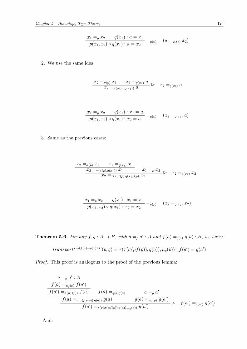
Chapter 5. Homotopy Type Theory 126
𝑥1 =𝑝 𝑥2 𝑞(𝑥1) : 𝑎 = 𝑥1 =𝜇(𝑝) (𝑎 =𝑞(𝑥2) 𝑥2)𝑝(𝑥1, 𝑥2) ∘ 𝑞(𝑥1) : 𝑎 = 𝑥2
2. We use the same idea:
𝑥2 =𝜎(𝑝) 𝑥1 𝑥1 =𝑞(𝑥1) 𝑎 B 𝑥2 =𝑞(𝑥2) 𝑎𝑥2 =𝜏(𝜎(𝑝),𝑞(𝑥1)) 𝑎
𝑥1 =𝑝 𝑥2 𝑞(𝑥1) : 𝑥1 = 𝑎 =𝜇(𝑝) (𝑥2 =𝑞(𝑥2) 𝑎)𝑝(𝑥1, 𝑥2) ∘ 𝑞(𝑥1) : 𝑥2 = 𝑎
3. Same as the previous cases:
𝑥2 =𝜎(𝑝) 𝑥1 𝑥1 =𝑞(𝑥1) 𝑥1𝑥2 =𝜏(𝜎(𝑝),𝑞(𝑥1)) 𝑥1 𝑥1 =𝑝 𝑥2 B 𝑥2 =𝑞(𝑥2) 𝑥2𝑥2 =𝜏(𝜏(𝜎(𝑝),𝑞(𝑥1)),𝑝) 𝑥2
𝑥1 =𝑝 𝑥2 𝑞(𝑥1) : 𝑥1 = 𝑥1 =𝜇(𝑝) (𝑥2 =𝑞(𝑥2) 𝑥2)𝑝(𝑥1, 𝑥2) ∘ 𝑞(𝑥1) : 𝑥2 = 𝑥2
Theorem 5.6. For any 𝑓, 𝑔 : 𝐴 → 𝐵, with 𝑎 =𝑝 𝑎′ : 𝐴 and 𝑓(𝑎) =𝑞(𝑎) 𝑔(𝑎) : 𝐵, we have:
𝑡𝑟𝑎𝑛𝑠𝑝𝑜𝑟𝑡𝑥→(𝑓(𝑥)=𝑔(𝑥)):𝐵(𝑝, 𝑞) = 𝜏(𝜏(𝜎(𝜇𝑓(𝑝)), 𝑞(𝑎)), 𝜇𝑔(𝑝)) : 𝑓(𝑎′) = 𝑔(𝑎′)
Proof. This proof is analogous to the proof of the previous lemma:
𝑎 =𝑝 𝑎′ : 𝐴
𝑓(𝑎) =𝜇𝑓 (𝑝) 𝑓(𝑎′)𝑓(𝑎′) =𝜎(𝜇𝑓 (𝑝)) 𝑓(𝑎) 𝑓(𝑎) =𝑞(𝑎)𝑔(𝑎)
𝑓(𝑎) =𝜏(𝜎(𝜇𝑓 (𝑝)),𝑞(𝑎)) 𝑔(𝑎)𝑎 =𝑝 𝑎
′
𝑔(𝑎) =𝜇𝑔(𝑝) 𝑔(𝑎′)B 𝑓(𝑎′) =𝑞(𝑎′) 𝑔(𝑎′)
𝑓(𝑎′) =𝜏(𝜏(𝜎(𝜇𝑓(𝑝)),𝑞(𝑎)),𝜇𝑔(𝑝)) 𝑔(𝑎′)
And:

Chapter 5. Homotopy Type Theory 127
𝑎 =𝑝 𝑎′ 𝑞(𝑎) : 𝑓(𝑎) = 𝑔(𝑎) =𝜇(𝑝) (𝑓(𝑎′) =𝑞(𝑎′) 𝑔(𝑎′))
𝑝(𝑎, 𝑎′) ∘ 𝑞(𝑎) : 𝑓(𝑎′) = 𝑔(𝑎′)
Theorem 5.7. For any 𝑓, 𝑔 : Π(𝑥:𝐴)𝐵(𝑥), with 𝑎 =𝑝 𝑎′ : 𝐴 and 𝑓(𝑎) =𝑞(𝑎) 𝑔(𝑎) : 𝐵(𝑎), we
have:
𝑡𝑟𝑎𝑛𝑠𝑝𝑜𝑟𝑡𝑥→(𝑓(𝑥)=𝑔(𝑥):𝐵(𝑥))(𝑝, 𝑞) = 𝜏(𝜏(𝜎(𝑎𝑝𝑑𝑓 (𝑝)), 𝜇𝑡𝑟𝑎𝑛𝑠𝑝𝑜𝑟𝑡𝐵𝑝(𝑞)), 𝑎𝑝𝑑𝑔(𝑝))
where 𝑎𝑝𝑑𝑓 (𝑝) ≡ (𝑝(𝑎, 𝑎′) ∘ 𝑓(𝑎) =𝜇(𝑝) 𝑓(𝑎′)) and 𝑎𝑝𝑑𝑔 ≡ (𝑝(𝑎, 𝑎′) ∘ 𝑔(𝑎) =𝜇(𝑝) 𝑔(𝑎′))
Proof. Similar to previous theorem:
𝑝(𝑎, 𝑎′) ∘ 𝑓(𝑎) =𝜇(𝑝) 𝑓(𝑎′)𝑓(𝑎′) =𝜎(𝜇(𝑝)) 𝑝(𝑎, 𝑎′) ∘ 𝑓(𝑎)
𝑓(𝑎) =𝑞(𝑎) 𝑔(𝑎)𝑝(𝑎, 𝑎′) ∘ 𝑓(𝑎) =𝜇
𝑡𝑟𝑎𝑛𝑠𝐵𝑝(𝑞(𝑎)) 𝑝(𝑎, 𝑎′) ∘ 𝑔(𝑎)
𝑓(𝑎′) =𝜏(𝜎(𝜇(𝑝)),𝜇𝑡𝑟𝑎𝑛𝑠𝐵𝑝
(𝑞(𝑎))) 𝑝(𝑎, 𝑎′) ∘ 𝑔(𝑎) 𝑝(𝑎, 𝑎′) ∘ 𝑔(𝑎) =𝜇(𝑝) 𝑔(𝑎′)𝑓(𝑎′) =𝜏(𝜏(𝜎(𝜇(𝑝)),𝜇
𝑡𝑟𝑎𝑛𝑠𝐵𝑝(𝑞(𝑎))),𝜇(𝑝) 𝑔(𝑎′)
B 𝑓(𝑎′) =𝑞(𝑎′) 𝑔(𝑎′)
And:
𝑎 =𝑝 𝑎′ 𝑞(𝑎) : 𝑓(𝑎) = 𝑔(𝑎)
B𝜇(𝑝) 𝑓(𝑎′) =𝑞(𝑎′) 𝑔(𝑎′)𝑝(𝑎, 𝑎′) ∘ 𝑞(𝑎) : 𝑓(𝑎′) = 𝑔(𝑎′)
Theorem 5.8. For any 𝑎 =𝑝 𝑎′ : 𝐴, 𝑎 =𝑞 𝑎 and 𝑎′ =𝑟 𝑎
′, we have:
(𝑡𝑟𝑎𝑛𝑠𝑝𝑜𝑟𝑡𝑥→(𝑥=𝑥)(𝑝, 𝑞) = 𝑟) ≃ (𝜏(𝑞, 𝑝) = 𝜏(𝑝, 𝑟))
Proof. We use lemma 5.20 to prove this theorem, together with rules 3,4,5,6 and 37. Wealso consider functions 𝑓(𝑥) ≡ 𝜏(𝑝, 𝑥) : (𝑎′ = 𝑧) → (𝑎 = 𝑧) and 𝑓−1(𝑥) ≡ 𝜏(𝜎(𝑝), 𝑥) : (𝑎 =𝑧) → (𝑎′ = 𝑧). We proceed the same way as we have done to prove previous equivalences.In other words, we show two derivations trees. They are as follows:
𝑡𝑟𝑎𝑛𝑠𝑝𝑜𝑟𝑡𝑥→(𝑥=𝑥)(𝑝, 𝑞) = 𝑟lemma 5.20
𝜏(𝜎(𝑝), 𝜏(𝑞, 𝑝)) = 𝑟𝜇𝑓
𝜏(𝑝, 𝜏(𝜎(𝑝), 𝜏(𝑞, 𝑝))) = 𝜏(𝑝, 𝑟)𝜏(𝜏(𝑝, 𝜎(𝑝)), 𝜏(𝑞, 𝑝)) = 𝜏(𝑝, 𝑟)
𝜏(𝜌, 𝜏(𝑞, 𝑝)) = 𝜏(𝑝, 𝑟)𝜏(𝑞, 𝑝) = 𝜏(𝑞, 𝑝)

Chapter 5. Homotopy Type Theory 128
And:
𝜏(𝑞, 𝑝) = 𝜏(𝑝, 𝑟)𝜇𝑓−1
𝜏(𝜎(𝑝), 𝜏(𝑞, 𝑝)) = 𝜏(𝜎(𝑝), 𝜏(𝑝, 𝑟))𝜏(𝜎(𝑝), 𝜏(𝑞, 𝑝)) = 𝜏(𝜏(𝜎(𝑝), 𝑝), 𝑟)
𝜏(𝜎(𝑝), 𝜏(𝑞, 𝑝)) = 𝜏(𝜏(𝜌, 𝑟)𝜏(𝜎(𝑝), 𝜏(𝑞, 𝑝)) = 𝑟
lemma 5.20𝑡𝑟𝑎𝑛𝑠𝑝𝑜𝑟𝑡𝑥→(𝑥=𝑥)(𝑝, 𝑞) = 𝑟
5.10 COPRODUCT
One essential thing to remember is that a product𝐴+𝐵 has a left injection 𝑖𝑛𝑙 : 𝐴 → 𝐴+𝐵and 𝑖𝑛𝑟 : 𝐵 → 𝐴+𝐵. As described in (Univalent Foundations Program, 2013), it is expectedthat 𝐴+𝐵 contains copies of 𝐴 and 𝐵 disjointly. In our path based approach, we achievethis by constructing every path 𝑖𝑛𝑙(𝑎) = 𝑖𝑛𝑙(𝑏) and 𝑖𝑛𝑟(𝑎) = 𝑖𝑛𝑟(𝑏) by applications ofaxiom 𝜇 on paths 𝑎 = 𝑏. Thus we show that we get the following equivalences:
1. (𝑖𝑛𝑙(𝑎1) = 𝑖𝑛𝑙(𝑎2)) ≃ (𝑎1 = 𝑎2)
2. (𝑖𝑛𝑟(𝑏1) = 𝑖𝑛𝑟(𝑏2)) ≃ (𝑏1 = 𝑏2)
3. (𝑖𝑛𝑙(𝑎) = 𝑖𝑛𝑟(𝑏)) ≃ 0
To prove this, we use the same idea as in (Univalent Foundations Program, 2013). Wecharacterize the type:
(𝑥 → (𝑖𝑛𝑙(𝑎0) = 𝑥)) : Π(𝑥:𝐴+𝐵)(𝑖𝑛𝑙(𝑎0 = 𝑥))
To do this, we define a type 𝑐𝑜𝑑𝑒:
𝑥 : 𝐴+𝐵 ⊢ 𝑐𝑜𝑑𝑒(𝑥) type
Our main objective is to prove the equivalence Π(𝑥:𝐴+𝐵)((𝑖𝑛𝑙(𝑎0) = 𝑥) ≃ 𝑐𝑜𝑑𝑒(𝑥)).Using the recursion principle of the coproduct, we can define 𝑐𝑜𝑑𝑒 by two equations:
𝑐𝑜𝑑𝑒(𝑖𝑛𝑙(𝑎)) ≡ (𝑎0 = 𝑎)𝑐𝑜𝑑𝑒(𝑖𝑛𝑟(𝑏)) ≡ 0
Theorem 5.9. For any 𝑥 : 𝐴+𝐵, we have 𝑖𝑛𝑙(𝑎0 = 𝑥) ≃ 𝑐𝑜𝑑𝑒(𝑥)
Proof. To show this equivalence, we use the same method as the one shown in (Univalent
Foundations Program, 2013). The main idea is to define functions

Chapter 5. Homotopy Type Theory 129
𝑒𝑛𝑐𝑜𝑑𝑒 : Π(𝑥:𝐴+𝐵)Π(𝑝:𝑖𝑛𝑙(𝑎0)=𝑥)𝑐𝑜𝑑𝑒(𝑥)𝑑𝑒𝑐𝑜𝑑𝑒 : Π(𝑥:𝐴+𝐵)Π(𝑐:𝑐𝑜𝑑𝑒(𝑥))(𝑖𝑛𝑙(𝑎0) = 𝑥))
such that 𝑑𝑒𝑐𝑜𝑑𝑒 acts as a quasi-inverse of 𝑒𝑛𝑐𝑜𝑑𝑒.We start defining 𝑒𝑛𝑐𝑜𝑑𝑒:
𝑒𝑛𝑐𝑜𝑑𝑒(𝑥, 𝑠) ≡ 𝑡𝑟𝑎𝑛𝑠𝑝𝑜𝑟𝑡𝑐𝑜𝑑𝑒(𝑠, 𝜌𝑎0)
We notice that 𝜌𝑎0 : 𝑐𝑜𝑑𝑒(𝑖𝑛𝑙(𝑎0)), since 𝑐𝑜𝑑𝑒(𝑖𝑛𝑙(𝑎0)) ≡ (𝑎0 =𝜌 𝑎0) We also noticethat for 𝑒𝑛𝑐𝑜𝑑𝑒, it is only possible for the argument 𝑥 to be of the form 𝑥 ≡ 𝑖𝑛𝑙(𝑎), sincethe other possibility is 𝑥 ≡ 𝑖𝑛𝑟(𝑎), but that case is not possible, because we would havea function to 𝑐𝑜𝑑𝑒(𝑖𝑛𝑟(𝑏)) ≡ 0.
For 𝑑𝑒𝑐𝑜𝑑𝑒, when 𝑥 ≡ 𝑖𝑛𝑙(𝑎), we have that 𝑐𝑜𝑑𝑒(𝑥) ≡ 𝑎0 =𝑐 𝑎 and thus, we definedecode as (𝑖𝑛𝑙(𝑎0) =𝜇(𝑐) 𝑖𝑛𝑙(𝑎)). When 𝑥 ≡ 𝑖𝑛𝑟(𝑎), then 𝑐𝑜𝑑𝑒(𝑥) ≡ 0 and thus, we define𝑑𝑒𝑐𝑜𝑑𝑒 as having any value, given by the elimination of the type 0. Now, we can finallyprove the equivalence.
Starting with 𝑒𝑛𝑐𝑜𝑑𝑒, we have 𝑥 ≡ 𝑖𝑛𝑙(𝑎), 𝑖𝑛𝑙(𝑎0) =𝑠 𝑥. Since𝑒𝑛𝑐𝑜𝑑𝑒(𝑥, 𝑠) ≡ 𝑡𝑟𝑎𝑛𝑠𝑝𝑜𝑟𝑡𝑐𝑜𝑑𝑒(𝑠, 𝜌𝑎0), we have:
𝑖𝑛𝑙(𝑎0) =𝑠 𝑖𝑛𝑙(𝑎) 𝜌𝑎0 : 𝑐𝑜𝑑𝑒(𝑖𝑛𝑙(𝑎0))𝑠(𝑖𝑛𝑙(𝑎0), 𝑖𝑛𝑙(𝑎)) ∘ 𝜌𝑎0 : 𝑐𝑜𝑑𝑒(𝑖𝑛𝑙(𝑎)) =𝜇(𝑠)
𝜌𝑎 : 𝑐𝑜𝑑𝑒(𝑖𝑛𝑙(𝑎)) ≡ 𝑐𝑜𝑑𝑒(𝑥)
Now, we can go back to 𝑖𝑛𝑙(𝑎0) = 𝑖𝑛𝑙(𝑎) by an application of 𝑑𝑒𝑐𝑜𝑑𝑒, since:
𝑑𝑒𝑐𝑜𝑑𝑒(𝜌𝑎 : 𝑐𝑜𝑑𝑒(𝑥)) ≡ 𝑖𝑛𝑙(𝑎0) =𝜇𝑖𝑛𝑙𝑖𝑛𝑙(𝑎)
And we conclude this part, since in our approach 𝑖𝑛𝑙(𝑎0) =𝑠 𝑖𝑛𝑙(𝑎) is constructed byapplications of axiom 𝜇.
Now, we start from decode. Let 𝑐 : 𝑐𝑜𝑑𝑒(𝑥). If 𝑥 ≡ 𝑖𝑛𝑙(𝑎), then 𝑐 : 𝑎0 = 𝑎 and thus,𝑑𝑒𝑐𝑜𝑑𝑒(𝑐) ≡ 𝑖𝑛𝑙(𝑎0) =𝜇(𝑐) 𝑖𝑛𝑙(𝑎). Now, we apply 𝑒𝑛𝑐𝑜𝑑𝑒. We have:
𝑒𝑛𝑐𝑜𝑑𝑒(𝑥, 𝜇𝑐) = 𝑡𝑟𝑎𝑛𝑠𝑝𝑜𝑟𝑡𝑐𝑜𝑑𝑒(𝜇𝑐, 𝜌𝑎0)= 𝑡𝑟𝑎𝑛𝑠𝑝𝑜𝑟𝑡𝑎→(𝑎0=𝑎)(𝑐, 𝜌𝑎0) (Lemma 11)= 𝜏(𝜌𝑎0 , 𝑐) (Lemma 20)= 𝑐 (Rule 6)
If 𝑥 ≡ 𝑖𝑛𝑟(𝑏), we have that 𝑐 : 0 and thus, as stated in (Univalent Foundations Program,2013), we can conclude anything we wish.

Chapter 5. Homotopy Type Theory 130
5.11 REFLEXIVITY
In this section, our objective is to conclude an important result related to the reflexivepath 𝜌:
Theorem 5.10. For any type A and a path 𝑥 =𝜌 𝑥 : 𝐴, if a path 𝑠 is obtained by a series(perhaps empty) of applications of axioms and rules of inference of 𝜆𝛽𝜂-equality theoryfor type theory to the path 𝜌, then there is a path 𝑡′ such that 𝑠 =𝑡′ 𝜌.
Proof. • Base Case:
We can start only with a path 𝑥 =𝜌. In that case, it is easy, since we have 𝜌 =𝜌 𝜌.Now, we consider the inductive steps. Starting from a path 𝑠 and applying 𝜏 , 𝜎, we
already have rules yield the desired path:
• 𝑠 = 𝜎(𝑠′), with 𝑠′ =𝑡′ 𝜌.
In this case, we have 𝑠 = 𝜎(𝑠′) = 𝜎(𝜌) =𝑠𝑟 𝜌.
• 𝑠 = 𝜏(𝑠′, 𝑠′′), with 𝑠′ =𝑡′ 𝜌 and 𝑠′′ =𝑡′′ 𝜌.
We have that 𝑠 = 𝜏(𝑠′, 𝑠′′) = 𝜏(𝜌, 𝜌) =𝑡𝑟𝑟 𝜌
The cases for applications of 𝜇, 𝜈 and 𝜉 remain to be proved. We introduce threenew rules that handle these cases.
• 𝑠 = 𝜇(𝑠′), with 𝑠′ =𝑡′ 𝜌.
We introduce rule 45:
𝑥 =𝜌𝑥 𝑥 : 𝐴 [𝑓 : 𝐴 → 𝐵]B𝑚𝑥𝑝 𝑓(𝑥) =𝜌𝑓(𝑥) 𝑓(𝑥) : 𝐵(𝑥)
𝑓(𝑥) =𝜇(𝜌𝑥) 𝑓(𝑥) : 𝐵(𝑥)
This rule is also valid for the dependent case:
𝑥 =𝜌𝑥 𝑥 : 𝐴 [𝑓 : Π(𝑥:𝐴)𝐵(𝑥)]B𝑚𝑥𝑝 𝑓(𝑥) =𝜌𝑓(𝑥) 𝑓(𝑥) : 𝐵(𝑥)
𝑝(𝑥, 𝑥) ∘ 𝑓(𝑥) =𝜇(𝜌𝑥) 𝑓(𝑥) : 𝐵(𝑥)
Thus, we have 𝑠 = 𝜇(𝑠′) = 𝜇(𝜌) =𝑚𝑥𝑝 𝜌.
• 𝑠 = 𝜈(𝑠′), with 𝑠′ =𝑡′ 𝜌.
We introduce rule 46:
𝑓 =𝜌 𝑓 : Π(𝑥:𝐴)𝐵(𝑥)B𝑛𝑥𝑝 𝑓(𝑥) =𝜌𝑓(𝑥) 𝑓(𝑥)
𝑓(𝑥) =𝜈(𝜌𝑥) 𝑓(𝑥) : 𝐵(𝑥)

Chapter 5. Homotopy Type Theory 131
Thus, 𝑠 = 𝜈(𝑠′) = 𝜈(𝜌) =𝑛𝑥𝑝 𝜌.
• 𝑠 = 𝜉(𝑠′), with 𝑠′ =𝑡′ 𝜌.
We introduce rule 47:
𝑏(𝑥) =𝜌 𝑏(𝑥) : 𝐵 𝑥 : 𝐴B𝑥𝑥𝑝 𝜆𝑥.𝑏(𝑥) =𝜌 𝜆𝑥.𝑏(𝑥)
𝜆𝑥.𝑏(𝑥) =𝜉(𝜌) 𝜆𝑥.𝑏(𝑥) : 𝐴 → 𝐵
Thus, 𝑠 = 𝜉(𝑠′) = 𝜉(𝜌) =𝑥𝑥𝑝 𝜌.
If we consider function extensionality, this theorem still holds:
• 𝑠 = 𝑒𝑥𝑡(𝑠′), with 𝑠′ =𝑡′ 𝜌.
We introduce a new rule to handle this case. Since it is related only to extensionality(i.e., when one admits the inference rule 𝑒𝑥𝑡 to the system), we do not add this tothe basic rules of our system.
𝜆𝑥.(𝑓(𝑥) =𝜌 𝑓(𝑥)) : Π(𝑥:𝐴)𝐵(𝑥)B𝑒𝑥𝑝 𝑓 =𝜌 𝑓
𝑓 =𝑒𝑥𝑡(𝜌) 𝑓
Thus, 𝑠 = 𝑒𝑥𝑡(𝑠′) = 𝑒𝑥𝑡(𝜌) =𝑒𝑥𝑝 𝜌.
5.12 NATURAL NUMBERS
The Natural Numbers is a type defined inductively by an element 0 : N and a function𝑠𝑢𝑐𝑐 : N → N. In our approach, the path space of the naturals is also characterizedinductively. We start from the reflexive path 0 =𝜌 0. All subsequent paths are constructedby applications of the inference rules of 𝜆𝛽𝜂-equality. We show that this characterizationis similar to the one constructed in (Univalent Foundations Program, 2013). To do this, we use𝑐𝑜𝑑𝑒, 𝑒𝑛𝑐𝑜𝑑𝑒 and 𝑑𝑒𝑐𝑜𝑑𝑒. For N, we define 𝑐𝑜𝑑𝑒 recursively (Univalent Foundations Program,2013):
𝑐𝑜𝑑𝑒(0, 0) ≡ 1𝑐𝑜𝑑𝑒(𝑠𝑢𝑐𝑐(𝑚), 0) ≡ 0𝑐𝑜𝑑𝑒(0, 𝑠𝑢𝑐𝑐(𝑚)) ≡ 0
𝑐𝑜𝑑𝑒(𝑠𝑢𝑐𝑐(𝑚), 𝑠𝑢𝑐𝑐(𝑛)) ≡ 𝑐𝑜𝑑𝑒(𝑚,𝑛)
We also define a dependent function 𝑟 : Π(𝑛:N)𝑐𝑜𝑑𝑒(𝑚,𝑛), with:

Chapter 5. Homotopy Type Theory 132
𝑟(0) ≡ *𝑟(𝑠𝑢𝑐𝑐(𝑛)) ≡ 𝑟(𝑛)
Theorem 5.11. For any 𝑚,𝑛 : N, if there is a path 𝑚 =𝑡 𝑛 : N, then 𝑡B 𝜌.
Proof. Since all paths are constructed from the reflexive path 0 =𝜌 0, this is a directapplication of theorem 5.10.
Theorem 5.12. For any 𝑚,𝑛 : N, we have (𝑚 = 𝑛) ≃ 𝑐𝑜𝑑𝑒(𝑚,𝑛)
Proof. We need to define 𝑒𝑛𝑐𝑜𝑑𝑒 and 𝑑𝑒𝑐𝑜𝑑𝑒 and prove that they are quasi-inverses. Wedefine 𝑒𝑛𝑐𝑜𝑑𝑒 : Π(𝑚,𝑛:N)(𝑚 = 𝑛) → 𝑐𝑜𝑑𝑒(𝑚,𝑛) as:
𝑒𝑛𝑐𝑜𝑑𝑒(𝑚,𝑛, 𝑝) ≡ 𝑡𝑟𝑎𝑛𝑠𝑝𝑜𝑟𝑡𝑐𝑜𝑑𝑒(𝑚,−)(𝑝, 𝑟(𝑚))
We define 𝑑𝑒𝑐𝑜𝑑𝑒 : Π(𝑚,𝑛:N)𝑐𝑜𝑑𝑒(𝑚,𝑛) → (𝑚 = 𝑛) recursively:
𝑑𝑒𝑐𝑜𝑑𝑒(0, 0, 𝑐) ≡ 0 =𝜌 0𝑑𝑒𝑐𝑜𝑑𝑒(𝑠𝑢𝑐𝑐(𝑚), 0, 𝑐) ≡ 0𝑑𝑒𝑐𝑜𝑑𝑒(0, 𝑠𝑢𝑐𝑐(𝑚), 𝑐) ≡ 0)
𝑑𝑒𝑐𝑜𝑑𝑒(𝑠𝑢𝑐𝑐(𝑚), 𝑠𝑢𝑐𝑐(𝑛), 𝑐) ≡ 𝜇𝑠𝑢𝑐𝑐(𝑑𝑒𝑐𝑜𝑑𝑒(𝑚,𝑛, 𝑐))
We now prove that if 𝑚 =𝑝 𝑛, then 𝑑𝑒𝑐𝑜𝑑𝑒(𝑐𝑜𝑑𝑒(𝑚,𝑛)) = 𝜌. We prove by induction.The base is trivial, since 𝑑𝑒𝑐𝑜𝑑𝑒(0, 0, 𝑐) ≡ 𝜌. Now, consider 𝑑𝑒𝑐𝑜𝑑𝑒(𝑠𝑢𝑐𝑐(𝑚), 𝑠𝑢𝑐𝑐(𝑛), 𝑐).We have that 𝑑𝑒𝑐𝑜𝑑𝑒(𝑠𝑢𝑐𝑐(𝑚), 𝑠𝑢𝑐𝑐(𝑛), 𝑐) ≡ 𝜇𝑠𝑢𝑐𝑐(𝑑𝑒𝑐𝑜𝑑𝑒(𝑚,𝑛, 𝑐)). By the inductive hy-pothesis, 𝑑𝑒𝑐𝑜𝑑𝑒(𝑚,𝑛, 𝑐) ≡ 𝜌. Thus, we need to prove that 𝜇𝑠𝑢𝑐𝑐 = 𝜌. This last step is astraightforward application of rule 47. Therefore, 𝜇𝑠𝑢𝑐𝑐 =𝑚𝑥𝑝 𝜌. With this information,we can start the proof of the equivalence.
For any 𝑚 =𝑝 𝑛, we have:
𝑒𝑛𝑐𝑜𝑑𝑒(𝑚,𝑛, 𝑝) ≡ 𝑡𝑟𝑎𝑛𝑠𝑝𝑜𝑟𝑡𝑐𝑜𝑑𝑒(𝑚,−)(𝑝, 𝑟(𝑚))
Thus:
𝑚 =𝑝 𝑛 𝑟(𝑚) : 𝑐𝑜𝑑𝑒(𝑚,𝑚) =𝜇(𝑝) (𝑟(𝑛) : 𝑐𝑜𝑑𝑒(𝑚,𝑛))𝑝(𝑚,𝑛) ∘ 𝑟(𝑚) : 𝑐𝑜𝑑𝑒(𝑚,𝑛)
Now, we know that 𝑑𝑒𝑐𝑜𝑑𝑒(𝑟(𝑛) : 𝑐𝑜𝑑𝑒(𝑚,𝑛)) = 𝜌 and,by theorem 5.11, 𝑝 = 𝜌.The proof starting from a 𝑐 : 𝑐𝑜𝑑𝑒(𝑚,𝑛) is equal to the one presented in (Univalent
Foundations Program, 2013). We prove by induction. If 𝑚 and 𝑛 are 0, we have the trivialpath 0 =𝜌 0, thus 𝑑𝑒𝑐𝑜𝑑𝑒(0, 0, 𝑐) = 𝜌0, whereas 𝑒𝑛𝑐𝑜𝑑𝑒(0, 0, 𝜌0) ≡ 𝑟(0) ≡ *. We con-clude this part recalling that every 𝑥 : 1 is equal to *, since we have 𝑥 =𝜎(𝜂) * : 1. Inthe case of 𝑑𝑒𝑐𝑜𝑑𝑒(𝑠𝑢𝑐𝑐(𝑚), 0, 𝑐) or 𝑑𝑒𝑐𝑜𝑑𝑒(0, 𝑠𝑢𝑐𝑐(𝑛), 𝑐), 𝑐 : 0. The only case left is for𝑑𝑒𝑐𝑜𝑑𝑒(𝑠𝑢𝑐𝑐(𝑚), 𝑠𝑢𝑐𝑐(𝑛), 𝑐). Similar to (Univalent Foundations Program, 2013), we prove byinduction:

Chapter 5. Homotopy Type Theory 133
𝑒𝑛𝑐𝑜𝑑𝑒(𝑠𝑢𝑐𝑐(𝑚), 𝑠𝑢𝑐𝑐(𝑛), 𝑑𝑒𝑐𝑜𝑑𝑒(𝑠𝑢𝑐𝑐(𝑚), 𝑠𝑢𝑐𝑐(𝑛), 𝑐))= 𝑒𝑛𝑐𝑜𝑑𝑒(𝑠𝑢𝑐𝑐(𝑚), 𝑠𝑢𝑐𝑐(𝑛), 𝜇𝑠𝑢𝑐𝑐(𝑑𝑒𝑐𝑜𝑑𝑒(𝑚,𝑛, 𝑐))= 𝑡𝑟𝑎𝑛𝑠𝑝𝑜𝑟𝑡𝑐𝑜𝑑𝑒(𝑠𝑢𝑐𝑐(𝑚),−)(𝜇𝑠𝑢𝑐𝑐(𝑑𝑒𝑐𝑜𝑑𝑒(𝑚,𝑛, 𝑐)), 𝑟(𝑠𝑢𝑐𝑐(𝑚))= 𝑡𝑟𝑎𝑛𝑠𝑝𝑜𝑟𝑡𝑐𝑜𝑑𝑒(𝑠𝑢𝑐𝑐(𝑚),𝑠𝑢𝑐𝑐(−)(𝑑𝑒𝑐𝑜𝑑𝑒(𝑚,𝑛, 𝑐), 𝑟(𝑠𝑢𝑐𝑐(𝑚)))= 𝑡𝑟𝑎𝑛𝑠𝑝𝑜𝑟𝑡𝑐𝑜𝑑𝑒(𝑚,−)(𝑑𝑒𝑐𝑜𝑑𝑒(𝑚,𝑛, 𝑐), 𝑟(𝑚))= 𝑒𝑛𝑐𝑜𝑑𝑒(𝑚,𝑛, 𝑑𝑒𝑐𝑜𝑑𝑒(𝑚,𝑛, 𝑐))= 𝑐
5.13 SETS AND AXIOM K
In this subsection, our objective is to prove, using our computational path approach,important results related to sets. First, We define the concept of set as done traditionallyin Homotopy Type Theory. Then, we show that the connection between the axiom K andsets is also valid in our approach. We use these results to show that the naturals numbersare a set. We also prove Hedberg’s theorem is valid in our theory, since only a few stepsof its proof differs from method developed in (Univalent Foundations Program, 2013).
We start with the definition of set (Univalent Foundations Program, 2013):
Definition 5.4. A type 𝐴 is a set if for all 𝑥, 𝑦 : 𝐴 and all 𝑝, 𝑞 : 𝑥 = 𝑦, we have 𝑝 = 𝑞.
In type theory, if a type is a set, we also say that it has the uniqueness of identityproof (UIP) property, since all proofs of the equality of two terms 𝑥 = 𝑦 are equal.
We now introduce the following axiom, known as axiom K(HOFMANN; STREICHER,1994):
For all 𝑥 : 𝑋 and 𝑝 : (𝑥 =𝑋 𝑥), we have 𝑝 = 𝑟𝑒𝑓𝑙𝑥.
Of course, this previous formulation is one familiar to classic type theory. In ourapproach, axiom K can be understood as the following formulation:
Axiom 5.2. For all 𝑥 : 𝑋 and 𝑥 =𝑡 𝑥 : 𝑋, we have 𝑡 = 𝜌𝑥.
Our objective is to establish a connection between sets and axiom K. The followinglemma has proved to be useful:
Lemma 5.21. For every path 𝑡, there is a path 𝑡−1 such that 𝑡 ∘ 𝑡−1 = 𝜌 and 𝑡−1 ∘ 𝑡 = 𝜌.Furthermore, 𝑡−1 is unique up to propositional identity.
Proof. We claim that 𝑡−1 = 𝜎(𝑡). The identities are straightforward. First, we have that𝑡 ∘ 𝑡−1 ≡ 𝜏(𝜎(𝑡), 𝑡) =𝑡𝑠𝑟 𝜌. We also have 𝑡−1 ∘ 𝑡 ≡ 𝜏(𝑡, 𝜎(𝑡)) =𝑡𝑟 𝜌. Now, suppose wehave 𝑠 such that 𝜏(𝑡, 𝑠) =𝑠′ 𝜌. Thus, we have that 𝜏(𝑡, 𝜎(𝑡)) =𝜏(𝑡𝑟,𝜎(𝑠′)) 𝜏(𝑡, 𝑠) and thus,𝜎(𝑡) = 𝑠.
Theorem 5.13. A type 𝑋 is a set iff it satisfies axiom K.

Chapter 5. Homotopy Type Theory 134
Proof. First, If 𝑋 is a set, we want to show that it satisfies axiom K. Suppose we havea path 𝑥 =𝑡 𝑥. From the axioms of 𝜆𝛽𝜂-equality, we also have that 𝑥 =𝜌 𝑥. Since 𝑋 is apath, it is always the case that 𝑡 = 𝜌 and thus, 𝑋 satisfies axiom K.
If𝑋 satisfies axiom K, we want to show that𝑋 is a set. To do this, we want to show thatgiven paths 𝑝, 𝑞 : 𝑥 = 𝑦, then we have 𝑝 = 𝑞. We show this in the following manner. From apath 𝑥 =𝑞 𝑦, we apply 𝜎 to obtain the inverse path 𝑦 =𝜎(𝑞)𝑥 𝑥. Then, we can concatenate 𝑝and 𝜎(𝑞), obtaining a path 𝑥 =𝜏(𝑝,𝜎(𝑞)) 𝑥. By axiom K, we have 𝜏(𝑝, 𝜎(𝑞)) = 𝜌. Analogously,𝜏(𝜎(𝑞), 𝑝) = 𝜌. Thus, by the previous lemma, 𝜎(𝑞) = 𝑝−1 = 𝜎(𝑝) and thus, 𝑞 = 𝑝. Thus,by an application of 𝜎, 𝑝 = 𝑞.
Theorem 5.14. N is a set.
Proof. That N satisfies axiom K is a direct consequence of theorem 5.11. Thus, fromtheorem 5.13, we conclude that N is a set.
In classic homotopy type theory, one can achieve the previous result by following adifferent path. Firstly, one should be aware of the following concept (Univalent Foundations
Program, 2013):
Definition 5.5. A type 𝑋 has decidable equality if for all 𝑥, 𝑦 : 𝑋, the following typeis inhabited:
(𝑥 = 𝑦 : 𝑋) + ¬(𝑥 = 𝑦 : 𝑋)
Theorem 5.15. If 𝑋 has decidable equality, then 𝑋 is a set.
This theorem is known as Hedberg’s theorem . We will not show a full proof of it,since one can follow exactly the steps established in (Univalent Foundations Program, 2013).One should only be careful to notice that the path 𝑎𝑝𝑑 of classic homotopy type theoryis just our application of axiom 𝜇 on a dependent function 𝑓 and that lemma 2.9.6 of(Univalent Foundations Program, 2013) has already been proved in this work, in the form oflemma 5.17.
We can also use Hedberg’s theorem to give an alternative proof of theorem 5.14, onesimilar to the one given in classic type theory:
Theorem 5.16. N has decidable equality and thus, is a set.
Proof. For any 𝑥, 𝑦 : N, we want to show that (𝑥 = 𝑦) + ¬(𝑥 = 𝑦) is inhabited. Weproceed by induction in 𝑥. For the base case, we have 𝑥 = 0. If 𝑦 = 0, then we have0 =𝜌 0. If 𝑦 = 𝑠𝑢𝑐𝑐(𝑛), we use the 𝑒𝑛𝑐𝑜𝑑𝑒 type for N. We have that 𝑒𝑛𝑐𝑜𝑑𝑒(0, 𝑠𝑢𝑐𝑐(𝑛)) :(0 = 𝑠𝑢𝑐𝑐(𝑛)) → 0 and thus, 𝑒𝑛𝑐𝑜𝑑𝑒(0, 𝑠𝑢𝑐𝑐(𝑛)) : ¬(0 = 𝑠𝑢𝑐𝑐(𝑛)).
For the inductive step, we consider 𝑥 = 𝑠𝑢𝑐𝑐(𝑚). If 𝑦 = 0, then we can use 𝑒𝑛𝑐𝑜𝑑𝑒 againto obtain ¬(𝑠𝑢𝑐𝑐(𝑚) = 0). If 𝑦 = 𝑠𝑢𝑐𝑐(𝑛), by the inductive hypothesis, we have two more

Chapter 5. Homotopy Type Theory 135
cases to consider. If 𝑚 = 𝑛, then we apply axiom 𝜇, and thus 𝑠𝑢𝑐𝑐(𝑚) =𝜇𝑠𝑢𝑐𝑐 𝑠𝑢𝑐𝑐(𝑛).If ¬(𝑚 = 𝑛), then we just need to show that 𝑠𝑢𝑐𝑐 is injective to obtain ¬(𝑠𝑢𝑐𝑐(𝑚) =𝑠𝑢𝑐𝑐(𝑛)). But that 𝑠𝑢𝑐𝑐 is injective is a direct consequence of applying encode and thendecode to 𝑠𝑢𝑐𝑐(𝑚) = 𝑠𝑢𝑐𝑐(𝑛), since from that we conclude 𝑚 = 𝑛. Therefore, from¬(𝑠𝑢𝑐𝑐(𝑚) = 𝑠𝑢𝑐𝑐(𝑛)) we conclude ¬(𝑚 = 𝑛).
5.14 FUNDAMENTAL GROUP OF A CIRCLE
The objective of this section is to show that it is possible to use computational paths toobtain one of the main results of homotopy theory, the fact that the fundamental groupof a circle is isomorphic to the integers group. First, we define a circle as follows:
Definition 5.6 (The circle 𝑆1). A circle is the type generated by:
• A point 𝑏𝑎𝑠𝑒 : 𝑆1
• A computational path 𝑏𝑎𝑠𝑒 =𝑙𝑜𝑜𝑝 𝑏𝑎𝑠𝑒 : 𝑆1.
The first thing one should notice is that this definition doest not use only the pointsof the type 𝑆1, but also a computational path 𝑙𝑜𝑜𝑝 between those points. That is way itis called a higher inductive type (Univalent Foundations Program, 2013). Our approach differsfrom the classic one on the fact that we do not need to simulate the path-space betweenthose points, since computational paths exist in the syntax of the theory. Thus, if onestarts with a path 𝑏𝑎𝑠𝑒 =𝑙𝑜𝑜𝑝 𝑏𝑎𝑠𝑒 : 𝑆1., one can naturally obtain additional paths applyingthe path-axioms 𝜌, 𝜏 and 𝜎. Thus, one has a path 𝜎(𝑙𝑜𝑜𝑝) = 𝑙𝑜𝑜𝑝−1, 𝜏(𝑙𝑜𝑜𝑝, 𝑙𝑜𝑜𝑝), etc. Inclassic type theory, the existence of those additional paths comes from establishing thatthe paths should be freely generated by the constructors (Univalent Foundations Program,2013). In our approach, we do not have to appeal for this kind of argument, since allpaths comes naturally from direct applications of the axioms.
With that in mind, one can define the fundamental group of a circle. In homotopy the-ory, the fundamental group is the one formed by all equivalence classes up to homotopy ofpaths (loops) starting from a point 𝑎 and also ending at 𝑎. Since the we use computationalpaths as the syntax counterpart in type theory of homotopic paths, we use it to proposethe following definition:
Definition 5.7 (Π1(𝐴, 𝑎) structure). Π1(𝐴, 𝑎) is a structure defined as follows:
Π1(𝐴, 𝑎) = {[𝑝𝑎𝑡ℎ]𝑟𝑤 | 𝑎 =𝑝𝑎𝑡ℎ 𝑎 : 𝐴}
We use this structure to define the fundamental group of a circle. We also need toshow that it is indeed a group.
Proposition 5.1. (Π1(𝑆, 𝑎), ∘) is a group.

Chapter 5. Homotopy Type Theory 136
Proof. The first thing to define is the group operation ∘. Given any 𝑎 =𝑟 𝑎 : 𝑆1 and𝑎 =𝑡 𝑎 : 𝑆1, we define 𝑟 ∘ 𝑠 as 𝜏(𝑠, 𝑟). Thus, we now need to check the group conditions:
• Closure: Given 𝑎 =𝑟 𝑎 : 𝑆1 and 𝑎 =𝑡 𝑎 : 𝑆1, 𝑟 ∘ 𝑠 must be a member of the group.Indeed, 𝑟 ∘ 𝑠 = 𝜏(𝑠, 𝑟) is a computational path 𝑎 =𝜏(𝑠,𝑟) 𝑎 : 𝑆1.
• Inverse: Every member of the group must have an inverse. Indeed, if we have a path𝑟, we can apply 𝜎(𝑟). We claim that 𝜎(𝑟) is the inverse of 𝑟, since we have:
𝜎(𝑟) ∘ 𝑟 = 𝜏(𝑟, 𝜎(𝑟)) =𝑡𝑟 𝜌
𝑟 ∘ 𝜎(𝑟) = 𝜏(𝜎(𝑟), 𝑟) =𝑡𝑠𝑟 𝜌
Since we are working up to 𝑟𝑤-equality, the equalities hold strictly.
• Identity: We use the path 𝑎 =𝜌 𝑎 : 𝑆1 as the identity. Indeed, we have:
𝑟 ∘ 𝜌 = 𝜏(𝜌, 𝑟) =𝑡𝑙𝑟 𝑟
𝜌 ∘ 𝑟 = 𝜏(𝑟, 𝜌) =𝑡𝑟𝑟 𝑟.
• Associativity: Given any members of the group 𝑎 =𝑟 𝑎 : 𝑆1, 𝑎 =𝑡 𝑎 and 𝑎 =𝑠 𝑎, wewant that 𝑟 ∘ (𝑠 ∘ 𝑡) = (𝑟 ∘ 𝑠) ∘ 𝑡:
𝑟 ∘ (𝑠 ∘ 𝑡) = 𝜏(𝜏(𝑡, 𝑠), 𝑟) =𝑡𝑡 𝜏(𝑡, 𝜏(𝑠, 𝑟)) = (𝑟 ∘ 𝑠) ∘ 𝑡
All conditions have been satisfied. (Π1(𝑆, 𝑎), ∘) is a group.
Thus, (Π1(𝑆, 𝑎), ∘) is indeed a group. We call this group the fundamental group of 𝑆1.Therefore, the objective of this section is to show that Π1(𝑆, 𝑎) ∼= Z.
Before we start developing this proof, the following lemma will prove to be useful:
Lemma 5.22. All paths generated by a path 𝑎 =𝑙𝑜𝑜𝑝 𝑎 : 𝑆 are 𝑟𝑤-equal to a path 𝑙𝑜𝑜𝑝𝑛,for a 𝑛 ∈ Z.
We have said that from a 𝑙𝑜𝑜𝑝, one freely generate different paths applying the com-position 𝜏 and the symmetry. Thus, one can, for example, obtain something such as𝑙𝑜𝑜𝑝 ∘ 𝑙𝑜𝑜𝑝 ∘ 𝑙𝑜𝑜𝑝−1 ∘ 𝑙𝑜𝑜𝑝.... Our objective with this lemma is to show that, in fact, thispath can be reduced to a path of the form 𝑙𝑜𝑜𝑝𝑛, for 𝑛 ∈ Z.
Proof. The idea is to proceed by induction on the number 𝑛 of loops, i.e., 𝑙𝑜𝑜𝑝𝑛. We startfrom a base 𝜌. For the base case, it is trivially true, since we define it to be equal to 𝑙𝑜𝑜𝑝0.From 𝜌, one can construct more complex paths by composing with 𝑙𝑜𝑜𝑝 or 𝜎(𝑙𝑜𝑜𝑝) oneach step. We have the following induction steps:
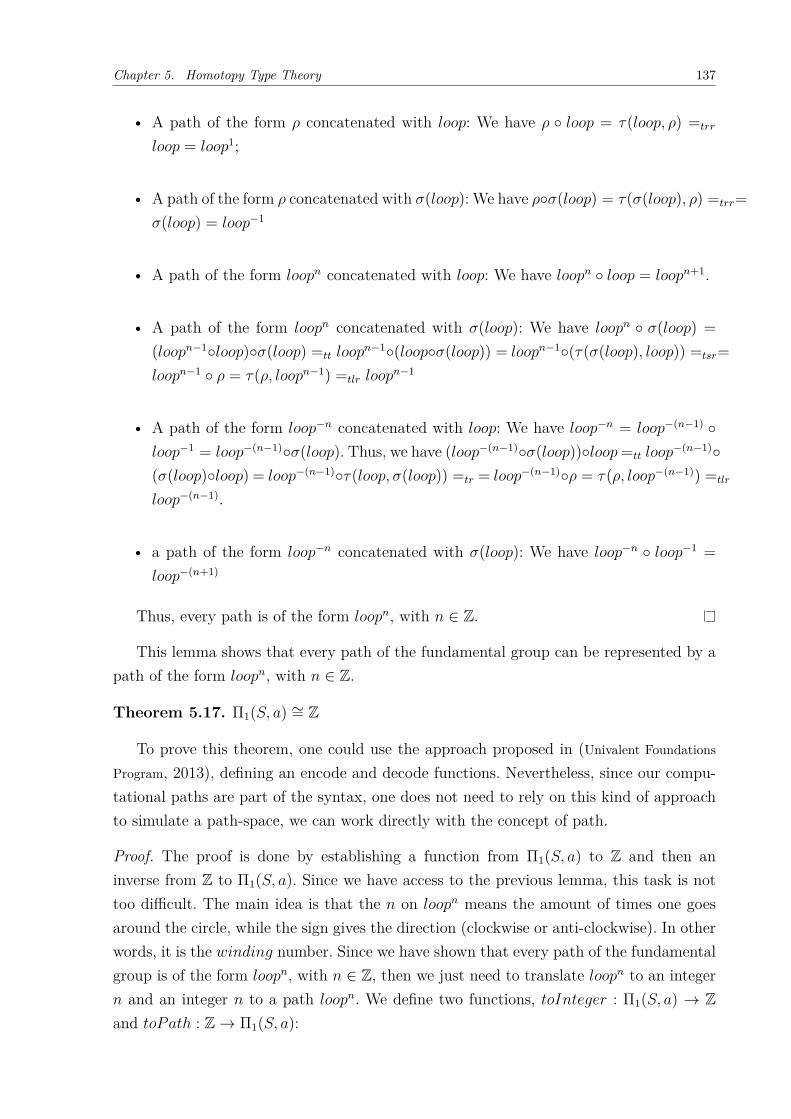
Chapter 5. Homotopy Type Theory 137
• A path of the form 𝜌 concatenated with 𝑙𝑜𝑜𝑝: We have 𝜌 ∘ 𝑙𝑜𝑜𝑝 = 𝜏(𝑙𝑜𝑜𝑝, 𝜌) =𝑡𝑟𝑟
𝑙𝑜𝑜𝑝 = 𝑙𝑜𝑜𝑝1;
• A path of the form 𝜌 concatenated with 𝜎(𝑙𝑜𝑜𝑝): We have 𝜌∘𝜎(𝑙𝑜𝑜𝑝) = 𝜏(𝜎(𝑙𝑜𝑜𝑝), 𝜌) =𝑡𝑟𝑟=𝜎(𝑙𝑜𝑜𝑝) = 𝑙𝑜𝑜𝑝−1
• A path of the form 𝑙𝑜𝑜𝑝𝑛 concatenated with 𝑙𝑜𝑜𝑝: We have 𝑙𝑜𝑜𝑝𝑛 ∘ 𝑙𝑜𝑜𝑝 = 𝑙𝑜𝑜𝑝𝑛+1.
• A path of the form 𝑙𝑜𝑜𝑝𝑛 concatenated with 𝜎(𝑙𝑜𝑜𝑝): We have 𝑙𝑜𝑜𝑝𝑛 ∘ 𝜎(𝑙𝑜𝑜𝑝) =(𝑙𝑜𝑜𝑝𝑛−1∘𝑙𝑜𝑜𝑝)∘𝜎(𝑙𝑜𝑜𝑝) =𝑡𝑡 𝑙𝑜𝑜𝑝
𝑛−1∘(𝑙𝑜𝑜𝑝∘𝜎(𝑙𝑜𝑜𝑝)) = 𝑙𝑜𝑜𝑝𝑛−1∘(𝜏(𝜎(𝑙𝑜𝑜𝑝), 𝑙𝑜𝑜𝑝)) =𝑡𝑠𝑟=𝑙𝑜𝑜𝑝𝑛−1 ∘ 𝜌 = 𝜏(𝜌, 𝑙𝑜𝑜𝑝𝑛−1) =𝑡𝑙𝑟 𝑙𝑜𝑜𝑝
𝑛−1
• A path of the form 𝑙𝑜𝑜𝑝−𝑛 concatenated with 𝑙𝑜𝑜𝑝: We have 𝑙𝑜𝑜𝑝−𝑛 = 𝑙𝑜𝑜𝑝−(𝑛−1) ∘𝑙𝑜𝑜𝑝−1 = 𝑙𝑜𝑜𝑝−(𝑛−1)∘𝜎(𝑙𝑜𝑜𝑝). Thus, we have (𝑙𝑜𝑜𝑝−(𝑛−1)∘𝜎(𝑙𝑜𝑜𝑝))∘𝑙𝑜𝑜𝑝=𝑡𝑡 𝑙𝑜𝑜𝑝
−(𝑛−1)∘(𝜎(𝑙𝑜𝑜𝑝)∘𝑙𝑜𝑜𝑝) = 𝑙𝑜𝑜𝑝−(𝑛−1)∘𝜏(𝑙𝑜𝑜𝑝, 𝜎(𝑙𝑜𝑜𝑝)) =𝑡𝑟 = 𝑙𝑜𝑜𝑝−(𝑛−1)∘𝜌 = 𝜏(𝜌, 𝑙𝑜𝑜𝑝−(𝑛−1)) =𝑡𝑙𝑟
𝑙𝑜𝑜𝑝−(𝑛−1).
• a path of the form 𝑙𝑜𝑜𝑝−𝑛 concatenated with 𝜎(𝑙𝑜𝑜𝑝): We have 𝑙𝑜𝑜𝑝−𝑛 ∘ 𝑙𝑜𝑜𝑝−1 =𝑙𝑜𝑜𝑝−(𝑛+1)
Thus, every path is of the form 𝑙𝑜𝑜𝑝𝑛, with 𝑛 ∈ Z.
This lemma shows that every path of the fundamental group can be represented by apath of the form 𝑙𝑜𝑜𝑝𝑛, with 𝑛 ∈ Z.
Theorem 5.17. Π1(𝑆, 𝑎) ∼= Z
To prove this theorem, one could use the approach proposed in (Univalent Foundations
Program, 2013), defining an encode and decode functions. Nevertheless, since our compu-tational paths are part of the syntax, one does not need to rely on this kind of approachto simulate a path-space, we can work directly with the concept of path.
Proof. The proof is done by establishing a function from Π1(𝑆, 𝑎) to Z and then aninverse from Z to Π1(𝑆, 𝑎). Since we have access to the previous lemma, this task is nottoo difficult. The main idea is that the 𝑛 on 𝑙𝑜𝑜𝑝𝑛 means the amount of times one goesaround the circle, while the sign gives the direction (clockwise or anti-clockwise). In otherwords, it is the 𝑤𝑖𝑛𝑑𝑖𝑛𝑔 number. Since we have shown that every path of the fundamentalgroup is of the form 𝑙𝑜𝑜𝑝𝑛, with 𝑛 ∈ Z, then we just need to translate 𝑙𝑜𝑜𝑝𝑛 to an integer𝑛 and an integer 𝑛 to a path 𝑙𝑜𝑜𝑝𝑛. We define two functions, 𝑡𝑜𝐼𝑛𝑡𝑒𝑔𝑒𝑟 : Π1(𝑆, 𝑎) → Zand 𝑡𝑜𝑃𝑎𝑡ℎ : Z → Π1(𝑆, 𝑎):

Chapter 5. Homotopy Type Theory 138
• 𝑡𝑜𝐼𝑛𝑡𝑒𝑔𝑒𝑟: To define this function, we use the help of two functions defined in Z:the successor function 𝑠𝑢𝑐𝑐 and the predecessor function 𝑝𝑟𝑒𝑑. We define 𝑡𝑜𝐼𝑛𝑡𝑒𝑔𝑒𝑟as follows. Of course, we use directly the fact that every loop of 𝑆 is of the form𝑙𝑜𝑜𝑝𝑛 with 𝑛 ∈ Z:
𝑡𝑜𝐼𝑛𝑡𝑒𝑔𝑒𝑟 :
⎧⎪⎪⎪⎪⎨⎪⎪⎪⎪⎩𝑡𝑜𝐼𝑛𝑡𝑒𝑔𝑒𝑟([𝑙𝑜𝑜𝑝𝑛]𝑟𝑤 ≡ [𝜌]𝑟𝑤) = 0 𝑛 = 0
𝑡𝑜𝐼𝑛𝑡𝑒𝑔𝑒𝑟([𝑙𝑜𝑜𝑝𝑛]𝑟𝑤) = 𝑠𝑢𝑐𝑐(𝑡𝑜𝐼𝑛𝑡𝑒𝑔𝑒𝑟([𝑙𝑜𝑜𝑝𝑛−1]𝑟𝑤)) 𝑛 > 0
𝑡𝑜𝐼𝑛𝑡𝑒𝑔𝑒𝑟([𝑙𝑜𝑜𝑝𝑛]𝑟𝑤) = 𝑝𝑟𝑒𝑑(𝑡𝑜𝐼𝑛𝑡𝑒𝑔𝑒𝑟([𝑙𝑜𝑜𝑝𝑛+1)]𝑟𝑤) 𝑛 < 0
• 𝑡𝑜𝑃𝑎𝑡ℎ: We just need to transform an integer 𝑛 into a path 𝑙𝑜𝑜𝑝𝑛:
𝑡𝑜𝑃𝑎𝑡ℎ :
⎧⎪⎪⎪⎪⎨⎪⎪⎪⎪⎩𝑡𝑜𝑃𝑎𝑡ℎ(𝑛) = [𝜌]𝑟𝑤 𝑛 = 0
𝑡𝑜𝑃𝑎𝑡ℎ(𝑛) = 𝑡𝑜𝑃𝑎𝑡ℎ(𝑛− 1) ∘ [𝑙𝑜𝑜𝑝]𝑟𝑤 𝑛 > 0
𝑡𝑜𝑃𝑎𝑡ℎ(𝑛) = 𝑡𝑜𝑃𝑎𝑡ℎ(𝑛+ 1) ∘ [𝜎(𝑙𝑜𝑜𝑝)]𝑟𝑤 𝑛 < 0
Now we just need to show that they are inverses. To do this, we have to check twoequations:
1. 𝑡𝑜𝑃𝑎𝑡ℎ(𝑡𝑜𝐼𝑛𝑡𝑒𝑔𝑒𝑟([𝑥]𝑟𝑤)) = [𝑥]𝑟𝑤
2. 𝑡𝑜𝐼𝑛𝑡𝑒𝑔𝑒𝑟(𝑡𝑜𝑃𝑎𝑡ℎ(𝑛)) = 𝑛
From a path [𝑥]𝑟𝑤, we apply lemma 5.22 to obtain [𝑥]𝑟𝑤 = [𝑙𝑜𝑜𝑝𝑛]𝑟𝑤 for some integer n.Thus, we have 𝑡𝑜𝑃𝑎𝑡ℎ(𝑡𝑜𝐼𝑛𝑡𝑒𝑔𝑒𝑟([𝑥]𝑟𝑤)) = 𝑡𝑜𝑃𝑎𝑡ℎ(𝑡𝑜𝐼𝑛𝑡𝑒𝑔𝑒𝑟([𝑙𝑜𝑜𝑝𝑛]𝑟𝑤)) = 𝑡𝑜𝑃𝑎𝑡ℎ(𝑛) =[𝑙𝑜𝑜𝑝𝑛]𝑟𝑤 = [𝑥]𝑟𝑤. The opposite direction is straightforward: 𝑡𝑜𝐼𝑛𝑡𝑒𝑔𝑒𝑟(𝑡𝑜𝑃𝑎𝑡ℎ(𝑛)) =𝑡𝑜𝐼𝑛𝑡𝑒𝑔𝑒𝑟([𝑙𝑜𝑜𝑝𝑛]𝑟𝑤) = 𝑛. Thus, we conclude that they are inverses. Also, the map be-tween the operations of the groups is direct, since we can easily map ∘ to +. This is due tothe fact that 𝑙𝑜𝑜𝑝𝑛 ∘ 𝑙𝑜𝑜𝑝𝑚 = 𝑙𝑜𝑜𝑝𝑛+𝑚 and thus, 𝑡𝑜𝐼𝑛𝑡𝑒𝑔𝑒𝑟[[𝑙𝑜𝑜𝑝𝑛+𝑚]𝑟𝑤 = 𝑛+𝑚. It is alsostraightforward that 𝑡𝑜𝑃𝑎𝑡ℎ(𝑛 + 𝑚) = [𝑙𝑜𝑜𝑝𝑛+𝑚]𝑟𝑤. Thus, we establish the isomorphismΠ1(𝑆, 𝑎) ∼= Z.
5.15 RULES ADDED TO 𝐿𝑁𝐷𝐸𝑄 − 𝑇𝑅𝑆
In this chapter, we have introduced 7 new rules to the 𝐿𝑁𝐷𝐸𝑄 − 𝑇𝑅𝑆 system. It is thefollowing list of rules:
40. 𝜏(𝜇(𝑟), 𝜇(𝑠)) =𝑡𝑓 𝜇(𝜏(𝑟, 𝑠))41. 𝜇𝑔(𝜇𝑓 (𝑝)) =𝑐𝑓 𝜇𝑔∘𝑓 (𝑝)42. 𝜇𝐼𝑑𝐴
(𝑝) =𝑐𝑖 𝑝
43. 𝜏(𝐻𝑓,𝑔(𝑥), 𝜇𝑔(𝑝)) =ℎ𝑝 𝜏(𝜇𝑓 (𝑝), 𝐻𝑓,𝑔(𝑦))44. 𝜇𝑓 (𝜖∧(𝑝, 𝑞)) =𝑚𝑥𝑐 𝜖∧(𝜇𝑔(𝑝), 𝜇ℎ(𝑞))

Chapter 5. Homotopy Type Theory 139
45. 𝜇𝑓 (𝜌𝑥) =𝑚𝑥𝑝 𝜌𝑓(𝑥)
46. 𝜈(𝜌𝑥) =𝑛𝑥𝑝 𝜌𝑓(𝑥)
47. 𝜉(𝜌) =𝑥𝑥𝑝 𝜌
Moreover, if one adds extensionality to the theory, one winds up with three additionalrules:
𝜈(𝑒𝑥𝑡(𝑡)) =𝑒𝑥𝑡𝑙 𝑡
𝜇𝑓 (𝜌𝑥) =𝑚𝑥𝑝 𝜌𝑓(𝑥)
𝑒𝑥𝑡(𝜌) =𝑒𝑥𝑝 𝜌.
Thus, we end this work with a total of 47 rewrites rules + 3 optional ones. Of course,to be formal we need to show that the system will terminate and is still confluent. Indeed,the confluence process can even yield new rules to solve some critical pair divergence. Weleave this verification out of the scope of this work, but given the importance of theseproofs, we plan to finish them in a future work.
5.16 CONCLUSION
In this chapter we have developed one of the main objectives of this work. We connectedour computational path approach to homotopy type theory. Using the algebra of compu-tational paths, we have established important results of Homotopy Type Theory. Thatway, we have shown that our approach yields the main building blocks of Homotopy TypeTheory, on par with the classic approach. We have also improved the rewrite system,adding new reduction rules. Indeed, we have ended this chapter with one of the mostclassic results of algebraic topology, the fact that the fundamental group of the circle isisomorphic to the group of the integers.
In view of all results achieved in this chapter, we have developed a valid alternativeapproach to the identity type and homotopy type theory, based on this algebra of paths.We also believe that we have opened the way, in future works, for possible expansionsof this results, formulating and proving even more intricate concepts and theorems ofhomotopy type theory using computational paths. In fact, based on the concepts developedin this chapter, we have constructed the fundamental group of many structures, includingthe Möbius band, the cylinder, torus and the projective plane. These results appear in astill unpublished work "On the Calculation of Fundamental Groups in Homotopy TypeTheory by Means of Computational Paths". A preprint version is available in (VERAS et
al., 2018).

140
6 CONCLUSION
Motivated by seeing the equality between two computational objects as a sequence ofrewrites between then, we have proposed in this work a entity known as computationalpaths. We have also accomplished 3 main objectives. The first one was the proposalof computational paths as an new entity of type theory. In this proposal, we pointedout the fact that computational paths should be seen as the syntax counterpart of thehomotopical paths between terms of a type. We have also proposed a formalization ofthe identity type using computational paths. The second objective was the proposal of amathematical structure for a type using computational paths. We have shown that usingcategorical semantics it was possible to induce a groupoid structure for a type and alsoa higher groupoid structure, using computational paths and a rewrite system. We haveused this groupoid structure to show that computational paths also refutes the uniquenessof identity proofs. The last objective was to formulate and prove the main concepts andbuilding blocks of homotopy type theory. We ended this last objective with a proof of theisomorphism between the fundamental group of the circle and the group of the integers.
The introduction of this work was focused on giving a brief introduction to the foun-dations of mathematics and a brief explanation why axiomatic set theory, 𝑍𝐹𝐶, is notsuitable of working as a foundation of computation. Thus, we have said that homotopytype theory is a suitable alternative, since it can be used as a foundation of mathematicsand computation at the same time. We have also pointed out that the identity type is themain concept of homotopy type theory, since it is responsible for the homotopical inter-pretation of a type. Nevertheless, we said that this interpretation is limited to a semanticalinterpretation, since there is no entity in the syntax of type theory that represents thosepaths. Thus, we said that the focus of this work is to add such entity to type theory,which is known as computational path.
The second chapter has been focused on introducing the basic concepts of type theory.In this chapter we have introduced the constructions of the main types, showing the for-mation, introduction, elimination and computation rules. We have also shown the currentapproach for the identity type using the constructor 𝐽 . We have also shown the use ofthose rules in practice, showing how one can use 𝐽 to construct basic types of type theory,such as the symmetry and transitivity properties of the identity type.
The third chapter focused on introducing the basic concepts of category theory. Wehave said that one of the objectives achieved here was the proposal of a mathematicalstructure for computational paths. To achieve that, we have used the framework of cate-gory theory. Thus, the needed concepts of this theory has been introduced in chapter 3.We have also shown some concepts of higher category theory, since we use then in chapter4 to construct a higher groupoid.

Chapter 6. Conclusion 141
The fourth chapter has been focused on introducing a new entity known as com-putational paths to the syntax of type theory. To achieve that, we have used conceptsdeveloped in chapter 2 and some basic concepts of 𝜆-calculus. After introducing the con-cept of computational paths, we have shown how one can formally define the identitytype using this entity. To do that, we show the formation, introduction, elimination andcomputation rules for the identity type. To make our approach clearer, we have used thisnewly introduced rules to construct three basic types of equality, the reflexivity, symmetryand transitivity. We also showed that the process of obtaining those constructions waseasier than using 𝐽 . After that, we have shown the existence of a rewrite system that es-tablishes equalities between two computational paths. We have also said that this systemdoes that by mapping all possible redundancies that can appear in a computational path.We also pointed out that this system is confluent and terminates. Thus, we have said thatit is possible to think of a strong normal form for a computational path. In the sequel,we have used the concepts of chapter 3 to construct a groupoid model for those compu-tational paths. We also have gone one step further, showing that it is possible to thinkof a higher groupoid structure. Moreover, we have put this groupoid structure togetherwith the existence of a strong normal form to show that this approach also refutes theuniqueness of identity proofs.
The fifth chapter has been focused on accomplishing the third objective of this work.In this chapter we have developed the main building blocks of homotopy theory usingcomputational paths. Instead of using path-induction in our proofs, we have used our al-gebra of paths based on our rewrite system. Proceeding that way, we have shown dozensof lemmas and theorems of homotopy type theory. Thus, we have shown that computa-tional paths are capable of developing this theory. We finished this chapter showing oneof the most classic proofs of algebraic topology: the fundamental group of the circle isisomorphic to the group of integers.
6.1 FUTURE WORK
Since we have successfully accomplished our main objectives, we hope that we have madea strong case for the power of computational paths in homotopy type theory. This ap-proach seems promising, since it has been possible to prove many lemmas and theorems ofhomotopy type theory. Also, another promising aspect is that our mathematical structuremirrors the one obtained using the traditional identity type.
Thus, with those results in mind, it is possible to obtain further results in two fronts:we can focus on the mathematical interpretation of computational paths. In this work, wehave limited our scope to bicategories, but it is possible, in the future, to go even further,adding more dimensions, eventually obtaining an important result: computational pathsshould be able of inducing a weak ∞-groupoid. We expect this fact, since this has beenrecently achieved using the traditional approach of the identity type (LUMSDAINE, 2009;

Chapter 6. Conclusion 142
BERG; GARNER, 2011). The other direction is to continue to develop the main conceptsand theorems of homotopy theory. We have shown dozens in chapter 5, but there aremany more results. Thus, we could focus on this and use our algebra of computationalpaths to obtain further results. In fact, based on the concepts developed in chapter 5, wehave constructed the fundamental group of many structures, including the Möbius band,the cylinder, torus and the projective plane. These results appear in a still unpublishedwork "On the Calculation of Fundamental Groups in Homotopy Type Theory by Meansof Computational Paths". A preprint version is available in (VERAS et al., 2018).

143
REFERENCES
ALAMA, J. The lambda calculus. In: ZALTA, E. N. (Ed.). The Stanford Encyclopediaof Philosophy. Spring 2015. [S.l.: s.n.], 2015.
AVIGAD, J. Philosophy of mathematics. In: BOUNDAS, C. (Ed.). The EdinburghCompanion to Twentieth-Century Philosophies. [S.l.]: Edinburgh University Press, 2007.p. 234–251.
AWODEY, S. Category theory. 2nd. ed. [S.l.]: Oxford University Press, 2010.
AWODEY, S. Category Theory Foundations. 2012. Category Theory Foundations,Lecture at Oregon Programming Languages Summer School, Eugene, Oregon.
BARKER-PLUMMER, D. Turing machines. In: ZALTA, E. N. (Ed.). The StanfordEncyclopedia of Philosophy. Summer 2013. [S.l.: s.n.], 2013.
BERG, B. van den; GARNER, R. Types are weak 𝜔-groupoids. Proceedings of theLondon Mathematical Society, Oxford University Press, v. 102, n. 2, p. 370–394, 2011.
BRIDGES, D.; PALMGREN, E. Constructive mathematics. In: ZALTA, E. N. (Ed.).The Stanford Encyclopedia of Philosophy. Winter 2013. [S.l.: s.n.], 2013.
CHENADEC, P. L. On the logic of unification. Journal of Symbolic computation,Elsevier, v. 8, n. 1, p. 141–199, 1989.
DERSHOWITZ, N. Orderings for term-rewriting systems. Theoretical computer science,Elsevier, v. 17, n. 3, p. 279–301, 1982.
DUMMETT, M. Elements of Intuitionism. [S.l.]: Oxford, 1977. (Oxford Logic Guides,v. 39). ISBN 978-0198505242.
HARPER, R. Type Theory Foundations. 2012. Type Theory Foundations, Lecture atOregon Programming Languages Summer School, Eugene, Oregon.
HINDLEY, J. R.; SELDIN, J. P. Lambda-calculus and combinators: an introduction.[S.l.]: Cambridge University Press, 2008.
HOFMANN, M.; STREICHER, T. The groupoid model refutes uniqueness of identityproofs. In: Logic in Computer Science, 1994. LICS’94. Proceedings., Symposium on.[S.l.]: IEEE, 1994. p. 208–212.
HOFMANN, M.; STREICHER, T. The groupoid interpretation of type theory. In:Twenty-five years of constructive type theory (Venice, 1995). New York: Oxford Univ.Press, 1998, (Oxford Logic Guides, v. 36). p. 83–111.
HORSTEN, L. Philosophy of mathematics. In: ZALTA, E. N. (Ed.). The StanfordEncyclopedia of Philosophy. Spring 2015. [S.l.: s.n.], 2015.
HOWARD, W. A. The formulas-as-types notion of construction. In: SELDIN, J. P.;HINDLEY, J. R. (Ed.). To H. B. Curry: Essays on Combinatory Logic, LambdaCalculus, and Formalism. [S.l.]: Academic Press, 1980. p. 479–490. Reprint of 1969article.
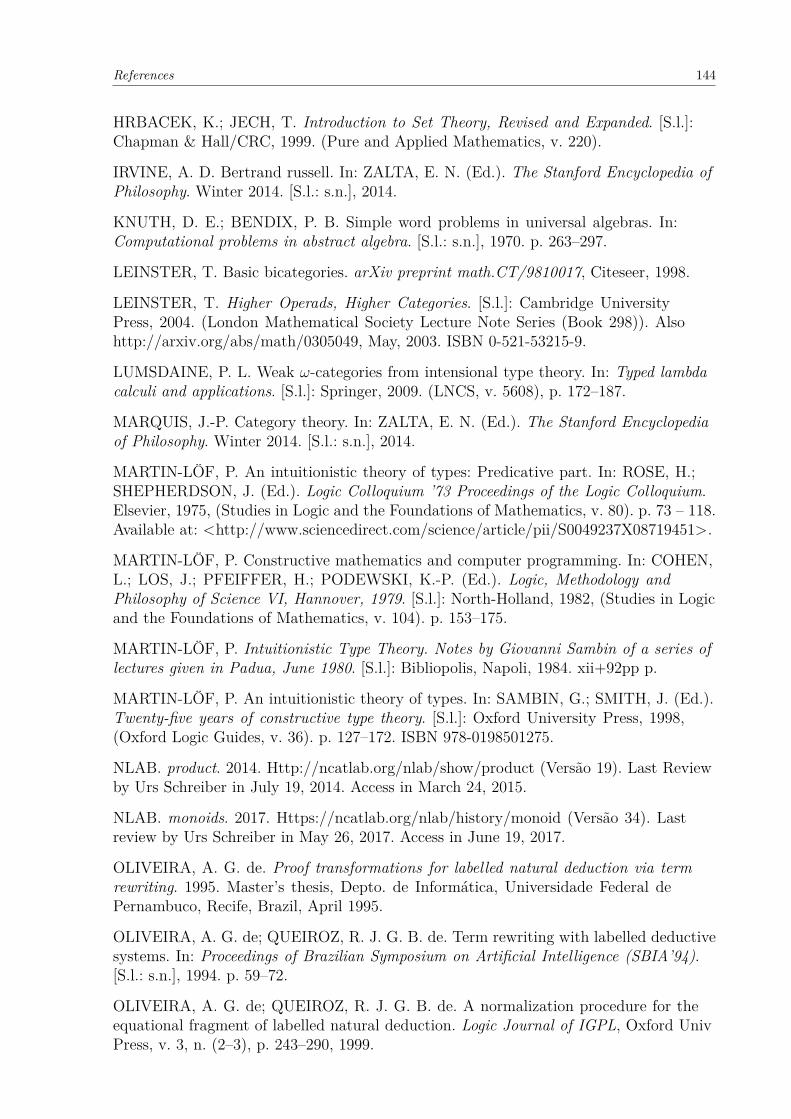
References 144
HRBACEK, K.; JECH, T. Introduction to Set Theory, Revised and Expanded. [S.l.]:Chapman & Hall/CRC, 1999. (Pure and Applied Mathematics, v. 220).
IRVINE, A. D. Bertrand russell. In: ZALTA, E. N. (Ed.). The Stanford Encyclopedia ofPhilosophy. Winter 2014. [S.l.: s.n.], 2014.
KNUTH, D. E.; BENDIX, P. B. Simple word problems in universal algebras. In:Computational problems in abstract algebra. [S.l.: s.n.], 1970. p. 263–297.
LEINSTER, T. Basic bicategories. arXiv preprint math.CT/9810017, Citeseer, 1998.
LEINSTER, T. Higher Operads, Higher Categories. [S.l.]: Cambridge UniversityPress, 2004. (London Mathematical Society Lecture Note Series (Book 298)). Alsohttp://arxiv.org/abs/math/0305049, May, 2003. ISBN 0-521-53215-9.
LUMSDAINE, P. L. Weak 𝜔-categories from intensional type theory. In: Typed lambdacalculi and applications. [S.l.]: Springer, 2009. (LNCS, v. 5608), p. 172–187.
MARQUIS, J.-P. Category theory. In: ZALTA, E. N. (Ed.). The Stanford Encyclopediaof Philosophy. Winter 2014. [S.l.: s.n.], 2014.
MARTIN-LÖF, P. An intuitionistic theory of types: Predicative part. In: ROSE, H.;SHEPHERDSON, J. (Ed.). Logic Colloquium ’73 Proceedings of the Logic Colloquium.Elsevier, 1975, (Studies in Logic and the Foundations of Mathematics, v. 80). p. 73 – 118.Available at: <http://www.sciencedirect.com/science/article/pii/S0049237X08719451>.
MARTIN-LÖF, P. Constructive mathematics and computer programming. In: COHEN,L.; LOS, J.; PFEIFFER, H.; PODEWSKI, K.-P. (Ed.). Logic, Methodology andPhilosophy of Science VI, Hannover, 1979. [S.l.]: North-Holland, 1982, (Studies in Logicand the Foundations of Mathematics, v. 104). p. 153–175.
MARTIN-LÖF, P. Intuitionistic Type Theory. Notes by Giovanni Sambin of a series oflectures given in Padua, June 1980. [S.l.]: Bibliopolis, Napoli, 1984. xii+92pp p.
MARTIN-LÖF, P. An intuitionistic theory of types. In: SAMBIN, G.; SMITH, J. (Ed.).Twenty-five years of constructive type theory. [S.l.]: Oxford University Press, 1998,(Oxford Logic Guides, v. 36). p. 127–172. ISBN 978-0198501275.
NLAB. product. 2014. Http://ncatlab.org/nlab/show/product (Versão 19). Last Reviewby Urs Schreiber in July 19, 2014. Access in March 24, 2015.
NLAB. monoids. 2017. Https://ncatlab.org/nlab/history/monoid (Versão 34). Lastreview by Urs Schreiber in May 26, 2017. Access in June 19, 2017.
OLIVEIRA, A. G. de. Proof transformations for labelled natural deduction via termrewriting. 1995. Master’s thesis, Depto. de Informática, Universidade Federal dePernambuco, Recife, Brazil, April 1995.
OLIVEIRA, A. G. de; QUEIROZ, R. J. G. B. de. Term rewriting with labelled deductivesystems. In: Proceedings of Brazilian Symposium on Artificial Intelligence (SBIA’94).[S.l.: s.n.], 1994. p. 59–72.
OLIVEIRA, A. G. de; QUEIROZ, R. J. G. B. de. A normalization procedure for theequational fragment of labelled natural deduction. Logic Journal of IGPL, Oxford UnivPress, v. 3, n. (2–3), p. 243–290, 1999.

References 145
QUEIROZ, R. J. G. B. de; GABBAY, D. The functional interpretation of the existentialquantifier. Bulletin of the IGPL, Oxford Univ Press, v. 7, n. 2, p. 173–215, 1995. (SpecialIssue on Deduction and Language, Guest Editor: Ruth Kempson). Full version of a paperpresented at Logic Colloquium ’91, Uppsala. Abstract in JSL 58(2):753–754, 1993.
QUEIROZ, R. J. G. B. de; GABBAY, D. M. Equality in labelled deductive systems andthe functional interpretation of propositional equality. In: DEKKER, P.; STOCKHOF,M. (Ed.). Proceedings of the 9th Amsterdam Colloquium. [S.l.], 1994. p. 547–565.
QUEIROZ, R. J. G. B. de; OLIVEIRA, A. G. de. Natural deduction for equality: Themissing entity. In: PEREIRA, L.; HAEUSLER, E.; PAIVA, V. de (Ed.). Advances inNatural Deduction. [S.l.]: Springer, 2014. p. 63–91.
QUEIROZ, R. J. G. B. de; OLIVEIRA, A. G. de. Propositional Equality, IdentityTypes and Reversible Rewriting Sequences as Homotopies. 2014. Propositional Equality,Identity Types and Reversible Rewriting Sequences as Homotopies, Talk at LogicWorkshop, Universidade Federal do Ceará, Fortaleza, CE, Brazil.
QUEIROZ, R. J. G. B. de; OLIVEIRA, A. G. de; GABBAY, D. M. The FunctionalInterpretation of Logical Deduction. [S.l.]: World Scientific, 2011.
QUEIROZ, R. J. G. B. de; OLIVEIRA, A. G. de; RAMOS, A. F. Propositional equality,identity types, and direct computational paths. South American Journal of Logic, v. 2,n. 2, p. 245–296, 2016. Special Issue: A Festschrift for Francisco Miraglia.
RAMOS, A. F. Identity Type as the Type of Computational Paths. 2015. Master’s thesis,Depto. de Informática, Universidade Federal de Pernambuco, Recife, Brazil, July, 2015.
RAMOS, A. F. Computational paths, transport and the univalence axiom. 2017. Talk atXVIII Brazilian Logic Conference, Pirenópolis, Goiás, May 2017.
RAMOS, A. F.; QUEIROZ, R. J. G. B. de; OLIVEIRA, A. G. de. On the identity typeas the type of computational paths. Logic Journal of IGPL, Oxford Univ Press, v. 3, n.(2–3), p. 243–290, 2017.
RAMOS, A. F.; QUEIROZ, R. J. G. B. de; OLIVEIRA, A. G. de. Explicit ComputationalPaths. 2018. Https://arxiv.org/abs/1609.05079.
Univalent Foundations Program. Homotopy Type Theory: Univalent Foundations ofMathematics. Institute for Advanced Study: <http://homotopytypetheory.org/book>,2013.
VERAS, T. M. L. de; RAMOS, A. F.; QUEIROZ, R. J. G. B. de; OLIVEIRA, A. G.de. On the Calculation of Fundamental Groups in Homotopy Type Theory by Means ofComputational Paths. 2018. Https://arxiv.org/abs/1804.01413.
VOEVODSKY, V. Univalent Foundations and Set Theory. 2014. Univalent Foundationsand Set Theory, Lecture at IAS, Princeton, New Jersey, Mar 2014.