artificial neural networks incorporating cost significant items towards enhancing...

Artificial Neural Networks Incorporating Cost Significant Items towards Enhancing Estimation for (life-cycle) Costing of Construction Projects

Ayedh Alqahtani and Andrew Whyte, (Curtin University, Australia)

Abstract Industrial application of life-cycle cost analysis (LCCA) is somewhat limited, with techniques deemed overly theoretical, resulting in a reluctance to realise (and pass onto the client) the advantages to be gained from objective LCCA comparison of (sub)component material specifications. To address the need for a user-friendly structured approach to facilitate complex processing, the work described here develops a new, accessible framework for LCCA of construction projects; it acknowledges Artificial Neural Networks (ANNs) to compute the whole-cost(s) of construction and uses the concept of cost significant items (CSI) to identify the main cost factors affecting the accuracy of estimation. ANN is a powerful means to handle non-linear problems and subsequently map relationships between complex input/output data and address uncertainties. A case study documenting 20 building projects was used to test the framework and estimate total running costs accurately. Two methods were used to develop a neural network model; firstly a back-propagation method using MATLAB SOFTWARE; and secondly, spread-sheet optimisation using Microsoft Excel Solver. The best network used 19 hidden nodes, with the tangent sigmoid used as a transfer function for both methods. The results is that in both models, the accuracy of the developed NN model is 1% (via Excel-solver) and 2% (via back-propagation) respectively. Keywords: Life Cycle Cost Analysis (LCCA), Artificial Neural Networks (ANNs), Cost Significant Items (CSIs), Back-propagation, Excel solver

Introduction

Stakeholders of built assets are increasingly required to extend estimation beyond the initial capital-cost. This includes all stages of an asset’s life-cycle, through incorporation of approaches such as benefit-to-cost ratio, internal rate of return and life cycle cost analysis (LCCA) to evaluate the total life cost of construction (Anurag Shankar et al. 2010). LCCA compares different design (sub)elements, specifications and materials on the basis of their whole-life installation, operation, maintenance and residual (decommissioning) costs. LCC analysis assesses all cost components, converting them into a cost at a specific point in time, namely the present (Olubodun et al. 2010). Client’s increasingly require such whole-costs for proposals. A key justification of LCCA use is the ability to reduce operation costs even if that requires spending more during early (construction) stages; expensive updating/retrofitting of older buildings is a significant factor encouraging LCCA uptake at the design development stage. However, Sterner (2000) argues that LCC influence is diminished by it’s perceived ‘uncertainty’; misunderstanding of the somewhat complex process alongside an absence of standardisation. There is also a need to acknowledge that market-trends limit the implementation of LCC concepts in industry (Olubodun et al. 2010, Sterner 2000), where calculations must consider the time-value of money, as all future costs requiring discounting to present-values taking inflation into account (Fabrycky and Blanchard 1991, Woodward 1997). Estimates of inflation and a

Australasian Journal of Construction Economics and Building

Alqahtani, A and Whyte, A (2013) ‘Artificial neural networks incorporating cost significant items towards enhancing estimation for (life-cycle) costing of construction projects’, Australasian Journal of Construction Economics and Building, 13 (3) 51-64

52

‘correct’ discount rate measuring the time-value-of-money so that design alternatives for a project, may be compared are deemed somewhat overly subjective, adding to uncertainty and risk and affecting LCC result accuracy. Indeed traditional methods remain restrictive, as LCC prediction of the large number of variable factors affects the ‘value’ of the construction cost, compounded by complicated interaction between these factors (Cheng et al. 2010), and coupled with the reluctance of busy practitioner’s to predict future discount-rate multipliers, continues to restrict LCCA usage by the construction industry. Many researchers recommend sensitivity and probability analyses, and statistical tools to address the problem of uncertainty (Singh 1990). Regression modelling is another method towards identification of construction cost impact factors, where regression equations estimate construction cost depending upon on cost-factor interrelationships. These methods become complex when numerous cost elements are considered as the dependent variables (Sonmez 2011). Sensitivity analysis is a method to indicate how the value of LCC is affected by changing the interest and inflation rate parameters. It is often the case where small variations in a parameter lead to a significant change in LCC result. In these cases a further analysis can be done utilizing probability analysis (Kirk 1995), incorporating Monte Carlo simulation of variables, presented as a probability distribution of all total costs of all alternative options. Resultant findings illustrate the most likely cost of all alternative options and the range within which it can be expected to lie (Flanagan and Norman 1993). However, these adaptations have disadvantages including:

i. Probability subjectively evaluated today may differ in the future (Whyte and Scott 2010). ii. Nominal account is taken of non-cost factors that affect LCC estimation. iii. Complex processes cannot fit input and output variables easily. iv. Sensitivity analysis does not quantify risk but rather identifies factors that are risk

sensitive where only one parameter is varied at a time (Flanagan and Norman 1993).

Towards addressing these uncertainties, the work presented here develops and tests a new model of estimating costs for each stage of a project, using Artificial Neural Networks (ANN) to estimate costs occurring at each stage of the life-cycle of construction. The model estimates the total capital, operation and maintenance costs, alongside an assessment of accuracy that compares total operation/maintenance costs of actual building projects.

Applications of ANNs in Construction Using simulation and modelling tools at all stages of an asset’s life cycle provides a way to anticipate the behaviour of an asset before it is built (Mackenzie and Briggs 2006). Artificial intelligence methods such as expert systems, neural networks (NNs), fuzzy logic (FL), and genetic algorithms (GAs) are argued to help solve prediction problems (Cheng et al. 2010). Artificial Neural Networks (ANNs) are data modelling methods that attempt to solve complicated issues by formulating data relationships; albeit that there is no simplistic equation that can map relationships between data variables. ANNs (in methods deemed to be similar to the performance of human brain) are beneficial where conditions are difficult to identify, and have been commonly employed in construction applications like estimating productivity; predicting corporate bankruptcy and measuring project financial performance. Indeed, a number of previous studies have sought to use neural networks to address construction estimation with varying degrees of success (Wilmot and Mei 2005); (Ehab et al. 2009);(Chang Sian et al. 2010);(Ali et al. 2011); (Ismaail et al. 2011);(Sodikov 2005);(Hashem Al-Tabtabai 1999);(Kim et al. 2004);(Arafa and Alqedra 2011);(Kim et al. 2005);(Murat Günaydın and Zeynep Doğan 2004)).



53

Previous study indicates that artificial neural networks are being considered for construction project estimation. Artificial Neural Networks (ANNs) with their ability to gain meaning from complicated data can be used to estimate costs that are too complicated to be solved by other techniques, with advantages of ANNs deemed to include that:

1. ANNs are capable of automatically learning how to perform work (by example) based on the information gathered for training; thus it is relatively easier to generate prediction models over other traditional nonlinear statistical methods;

2. ANNs whilst unable to explain explicitly the relationships between input and output variables, a main objective for creating a decision model is to be able to estimate and more accurately explain relations between variables;

3. ANNs are able to create the estimation model based on data forms of ordinal data or mixed forms of nominal and ordinal data; and in addition,

4. ANN generalisations are beneficial, as they utilise data that the model has collected during training stages to synthesize input-output mapping with new data.

Currently, building sector clients seek predictions that are flexible and easy to use. As mentioned before, ANNs have several advantages over traditional methods but there are currently no clear steps that can be followed to simplify the estimation cost process in ANNs applications. There is still a need to develop a framework of ANNs to (excite clients, and) predict whole construction costs. To make sense of the huge number of variable factors that affect the value of the construction cost; there is a need to provide better interaction between these factors in a less complicated process. It is important to standardise the estimation process and integrate some methods with ANNs, to identify the key factors to be considered as input factors of ANNs model. This research will develop a new framework for estimation cost using artificial neural networks integration techniques.

New Framework towards a Cost Estimation Model The process developed here for a new model of cost estimation follows a number of systemic procedures. There are eight basics steps proposed here: (1) Identify the purpose of estimation; (2) identify cost factors affecting cost estimation; (3) identify non-cost factors affecting cost estimation; (4) Create database for cost and non-cost factors; (5)design NNS; (6) train NNs; (7) validation the model; and (8) run the application. See figure 1 and the text below:

Identification of the Purpose of Estimation The purpose of estimation may range from an estimate of construction cost only, to estimating the total life-cycle costs of new projects which include construction, operation and maintenance.

Implementation of CSIs: Construction projects have numerous variable factors impacting upon the value of LCC. Interaction between factors is somewhat complex with current LCC models suffering arguably from an absence of both standardisation and a simple methodology to collect and interpolate data (Olubodun et al. 2010). The concept of Cost-Significant-Items (CSIs) shall help future analysts to simplify estimation methodologies by determining the key items contributing most to construction project LCC. CSI ideology owes much to Pareto’s classic 80:20 rule. In the construction sector, various building-sector scholars have applied CSIs to construction cost estimate research, finding that CSIs theory is able to determine the small number of items which represent a constant percentage of the total cost of construction projects (Al-Hajj and Horner 1998, Asif 1988, Elcin and Hakan 2005, Horner and Zakieh 1996). If the CSIs could be simply



54

recognized, it would motivate estimators to direct attention to such specific items, and would reduce the time taken for estimation. In this way, cost information required to estimate total cost could be collected, analysed and recorded in a manner which will provide a more significant and realistic method of prediction.

Create database

Design NNs

CSIs

Training and

testing NNs

Final model of

NNs

Non-cost

factors

Purpose of estimation

Figure 1 Framework of NNs model

Identification of Non-Cost Factors affecting the Accuracy of Estimation: A main restriction of most of the current models of cost estimation is that they only consider significant factors that can be readily quantified. However, non-cost factors should be considered because they seem to play a vital and important role to the accuracy of cost estimation(Elhag et al. 2005). Non-cost factors affecting the accuracy of estimating come from a large range of categories. These factors are qualitative such as type of project (residential, commercial, industrial), type of structure (concrete, steel, masonry), and project size. These factors can be identified from an analysis of literature, historical data and practitioner experience.

Database Creation Database creation consists of taking the most significant cost/non-cost factors, already identified in earlier steps and actual values of unit-rate costs for past projects. This data is used to exemplify input and output information in the proposed model during the training/testing stages.

Design of Neural Networks The initial steps in the design of neural network modelling are selecting, collecting and preparing suitable data. In estimation cost modelling, there are two types of data needed to create a neural network model: input data consisting of data identified as key to the result of the cost estimation model (collected from the database) representing CSIs and the important non-cost factors; and output data consisting of the data collected from the database representing the actual value of total costs of previous projects. Such data needs to be normalized before



55

presented to the network, because mixing variables with big magnitudes and small magnitudes will confuse the learning algorithm (Tymvios et al. 2008). The input and output data can be scaled to a range (-1 to 1) to suit neural networks processes. Normalization of the data uses the following formula (Arafa and Alqedra 2011):

= ⌈ ( )

⌉……… (1)

Where : Normal value, : Original data set, : the minimum value of data, : the maximum value of data.

After collecting the data, the designer specifies the number of hidden layers; neurons in each layer and transfer functions. In general, traditional parametric ‘trial & error’ is performed to select the number of hidden layers and hidden nodes. During the training process, the number of hidden layers and hidden nodes will be adjusted until identification of the best model which gives the lowest values for the Root Mean Square Error (RMS) and absolute difference percentage for output parameters. Transfer functions then describe how the neuron's activation value occurs as a result of applying a transfer function to the sum of the weighted inputs. Key transfer functions are the sigmoid, threshold and linear functions (Duch and Jankowski 1999).

Training and Testing NNs Training the neural network refers to a procedure that utilises numerous learning methods to

adjust weights and to learn patterns in the data-set, including iteratively gathering data with

samples of known right answers. Before starting the process of training, learning rates should

be selected. In fact, several ANNs programs, such as MATLAB, automatically set the learning

rate in terms of maximised performance of the model, to gain the best result. Regarding training

the model, training methods mostly fall into one of two categories: a supervised training method

in which the trainer tells the model if its result were correct; and an unsupervised training

method in which there is neither teacher nor trainer during training to tell the network whether its

output was correct. The network’s weights are continuously modified until the difference

between the model’s outputs and the actual output converges to an acceptable level. The

training process is stopped when a minimum root mean square error in equation 2 is reached.

√∑

( )2……………… (2)

where: RMS: root mean square error, n: number of sample using in the training stage, O i: the actual output. Pi: The model output.

Testing the model process is fundamentally the same as the training process, but the model will use sample (data) never seen before, and no corrections are made. If the results of a testing process are acceptable the model is suitable to use. If the result is inappropriate, a re-design of the model is required. The acceptable level of the result of the model will be evaluated based on the value of RMS (equation2) and absolute difference (in equation 3).

………. (3)

where: Oi: the actual output. Pi: The model output.



56

Final Model of ANNs: Once the model is built, it can be utilised to predict the cost of new construction projects. It should be noted that a building practitioner is then able to use the final model to estimate new project costs without performing changes to the design structure of the ANNs model such as the transfer function, the number of inputs (important cost and non-cost factors) and hidden nodes, which had been selected at an initial stage.

Case Study The Purpose of Estimation The aim of the following case study is to review/validate the newly developed framework for an estimation cost model for building projects. This case study aims to estimate the running costs (operation and maintenance costs) for three types of building projects (teaching, residential and laboratory facilities). The new work presented by this current study uses a comprehensive catalogue of 20 building projects compiled previously by Al-Hajj (1991). Al-Hajj’s cost information is documented as stemming from three sources, namely: York University; an independent facilities management company; and the UK’s Building Maintenance Cost Information Service (BMCIS-UK); the relevance of the case-study prepares the ground for future-work, described below.

Implementation of CSIs: The key cost factors affecting the accuracy of running-cost estimation for the twenty (teaching, residential and laboratory facility) building projects catalogued by Al-Hajj(1991), employing an analysis of cost significant items (CSIs) (across an existing data-set of 20 projects towards verification of the concept of Pareto), finds 11 items as most influential across all building projects over the catalogue’s analysis period of 18 years. These key items represent about 16% of all total items. Table (1) below lists the resultant cost significant items for the data-set:

CSIs (affecting the accuracy of running cost estimation)

1. Internal decoration

2. Roof repair

3. Internal cleaning

4. Laundry

5. Gas expenditure

6. Electricity expenditure

7. Fuel oil expenditure

8. Management fees

9. Porterage

10. Rates

11. Insurance

Table 1 cost significant items

Identification of Design Factors influencing Estimation Accuracy Seven major design factors from Al Hajj’s (1991) catalogue of 20 building projects, described as the most important design factors affecting building’s estimation cost, are listed in table 2 below.



57

Design Factors

1. Type of building

2. Gross Floor Area (m2)

3. Area of Pitched Roof (m2)

4. Area of Flat Roof (m2)

5. Area of External Glazing (m2)

6. Number of Stories Above Ground Floor

7. Number of Stories Under Ground Floor

Table 2 non-cost significant factors

Design Neural Networks a) Selection NNs software/simulation and data collection This paper compares two methods to create and design neural networks:

1- back-propagation method using MATLAB SOFTWARE (2012b) 2- spread sheet optimization using Microsoft Excel Solver.

Both methods use three-layer NN, because it is argued here that they provide simple transparent methods towards NN modelling. The neural network model developed in this paper consists of three layers (as figure 2 below): 1- Input layer of 8 nodes: type of building, gross floor area, area of pitched roof, area of flat

roof, area of external glazing, number of stories above ground floor, number of stories under ground floor and CSIs.

2- hidden layer (trial and error in a training stage used to determine number of nodes) 3- Output layer contained one node (the total running cost).

Figure 2 neural network structure with three layers

The data for the 20 projects were entered into Excel. The input and output data is normalized and scaled to a range (-1 to 1) using equation 1 to suit neural networks processes. b) Determining the best network architecture Traditional parametric (trial and error) has been performed to select the number of hidden layers and the number of hidden nodes. During the training process, the number of hidden layers and hidden nodes are adjusted to find the best artificial neural network model to give the lowest value for the Root Mean Square (RMS) and absolute difference percentage for output parameters. Tangent Sigmoid is used as a transfer function of NNs model for both methods. In



58

order to train/test the model and find a best number of nodes in hidden layers, MATLAB is utilised for its ease of use and speed of training. The best architecture resulting from MATLAB is compiled to spread sheet to compare the results of both methods. c) Training and testing the network In this case study, the 20 projects are divided to three sets. One set consist of 14 projects (70%) used for training the model and 3 projects (15%) are used towards model validation and the remaining 3 projects (15%) used to test the procedure. As mentioned before, one of the objectives of training the model is to identify the best structure of neural network model. The acceptable level of the result of the model is evaluated based on the value of RMS (equation2) and absolute difference (in equation 3).

Results a) back-propagation The back-propagation method, the ‘weights’ which aim to connect nodes and biases are changed utilising a number of inputs and the desired output value. The difference between the network output and actual output, become network error sets, after which the network error is back propagated from the output layer to adjust the weights and biases. This step is repeatedly performed until the minimum level of network error is reached. The 20 model trails and error were applied to identify the number of hidden nodes on hidden layers. It was clear that increasing the number of hidden nodes in hidden layers leads to changing the value of RMS and Absolute Difference error. 19 hidden nodes provided the lowest RMS value of 0.033 and an absolute difference error value of 0.96%. However, neural network models with one hidden node provided the highest RMS value of 0.388 with an absolute difference error value of 3.89%. The value of RMS & absolute difference error changed consecutively within the above mentioned range for the remaining 18 model trails. Table 3 below illustrates RMS and an absolute difference error for all 20 model trails.

Table 3 20 model trails for determining the best model

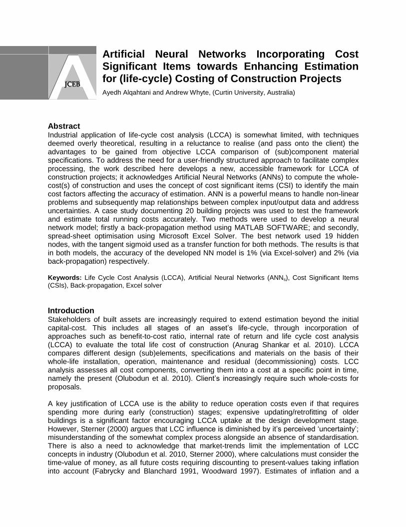
Figure 3 below present the properties of the best neural network model gained through the trial and error method at a training stage.

No. of hidden

nodes

RMS % Absolute different

error

No. of hidden

nodes


error

No. of hidden

nodes


error

1 0.388 3.89 8 0.062 1.08 15 0.089 1.61

2 0.096 3.10 9 0.094 2.21 16 0.106 1.51

3 0.174 5.25 10 0.063 1.42 17 0.206 4.82

4 0.093 1.74 11 0.057 0.79 18 0.069 1.04

5 0.129 1.80 12 0.324 8.59 19 0.033 0.96

6 0.054 1.02 13 0.045 1.03 20 0.324 6.94

7 0.116 2.57 14 0.047 1.18



59

Figure 3 Structure of the Best Model

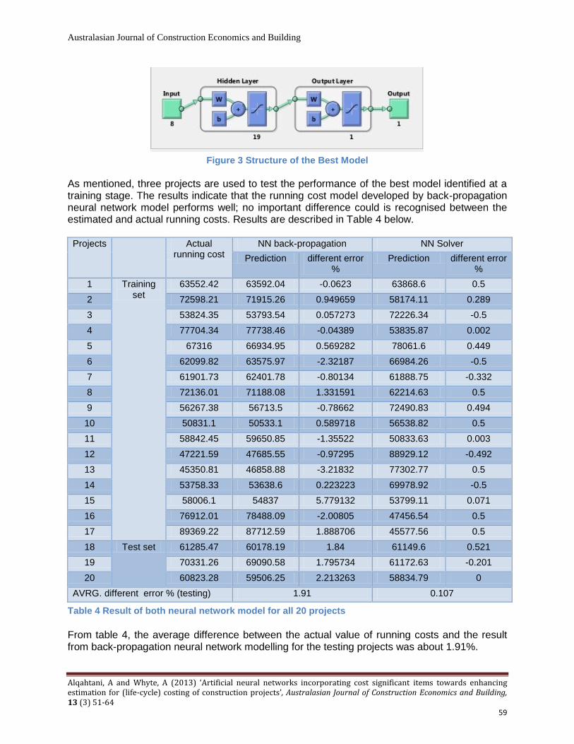
As mentioned, three projects are used to test the performance of the best model identified at a training stage. The results indicate that the running cost model developed by back-propagation neural network model performs well; no important difference could is recognised between the estimated and actual running costs. Results are described in Table 4 below. Projects Actual

running cost NN back-propagation NN Solver

Prediction different error %

Prediction different error %

1 Training set

63552.42 63592.04 -0.0623 63868.6 0.5

2 72598.21 71915.26 0.949659 58174.11 0.289

3 53824.35 53793.54 0.057273 72226.34 -0.5

4 77704.34 77738.46 -0.04389 53835.87 0.002

5 67316 66934.95 0.569282 78061.6 0.449

6 62099.82 63575.97 -2.32187 66984.26 -0.5

7 61901.73 62401.78 -0.80134 61888.75 -0.332

8 72136.01 71188.08 1.331591 62214.63 0.5

9 56267.38 56713.5 -0.78662 72490.83 0.494

10 50831.1 50533.1 0.589718 56538.82 0.5

11 58842.45 59650.85 -1.35522 50833.63 0.003

12 47221.59 47685.55 -0.97295 88929.12 -0.492

13 45350.81 46858.88 -3.21832 77302.77 0.5

14 53758.33 53638.6 0.223223 69978.92 -0.5

15 58006.1 54837 5.779132 53799.11 0.071

16 76912.01 78488.09 -2.00805 47456.54 0.5

17 89369.22 87712.59 1.888706 45577.56 0.5

18 Test set 61285.47 60178.19 1.84 61149.6 0.521

19 70331.26 69090.58 1.795734 61172.63 -0.201

20 60823.28 59506.25 2.213263 58834.79 0

AVRG. different error % (testing) 1.91 0.107

Table 4 Result of both neural network model for all 20 projects

From table 4, the average difference between the actual value of running costs and the result from back-propagation neural network modelling for the testing projects was about 1.91%.



60

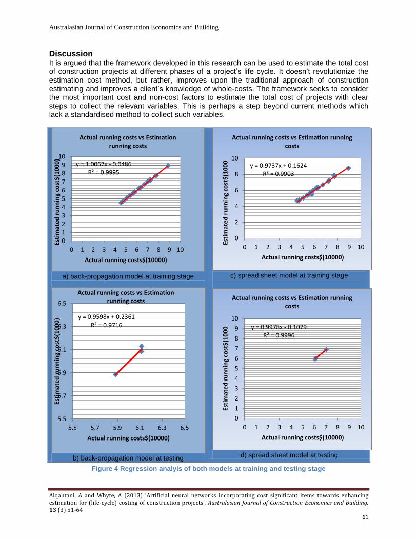
b) Spread sheet using Excel Solver ‘Solver’ finds the best set of values for some variables by maximizing or minimizing a desired output cell connected by formulas to the variables, under a set of user-specified constraints. In this case, the optimization goal is to reduce the NN weighted error to 0. In order to reach this goal, the adjustable variable has been identified as the weights from inputs to hidden nodes and from hidden nodes to outputs. Optimization constraints were set to limit the percentage error on both training and test project to 3% and 1% or lower to avoid erroneous network result on individual training projects. This paper applied 7 steps as suggested by Hegazy and Ayed (1998) to build ANNs model in spread sheet. The best architecture resulting from MATLAB was used on the spread sheet (8 nodes on input layer-19 nodes in hidden layers-1 node on output layers). 17 projects were used to train the model and 3 projects were used to test the model (the same 3 projects that were used to test back-propagation modelling). The results show that the running cost model developed by spread sheet neural network modelling performs well. No important differences are recognised between the estimated and actual running costs (table 4). From table 4 the average difference between the actual value of running costs and the result from spread sheet neural network modelling for the testing projects was 0.107%. The expected accuracy of the both models at training and testing stage is introduced in table 5 below. The spread-sheet neural network model and back- propagation are able to estimate the total running cost with an average accuracy of 99% and 98%. The neural network model results from both the training and testing stages and the actual value of running costs for both models were analysed through regression analysis in order to investigate the model response in more detail. The result of linearly regression is presented graphically in figure 4 below. Liner regression analysis consists of two parameters (as equation 4).

Y (actual value) = m*X (estimated value) + b…………………………….(4)

where m & b represent the slope and the y-intercept of the best regression relating the actual value of running costs to the neural network model. For both models, in both training and testing stages, the slope is close to1 and the y-intercept is close to 0, indicating a good fit. In addition, regression analysis is able to provide the value of the correlation coefficient (R2) between the actual value of running cost and the model output. For both models, in training and testing tests, R2 is close to 1, indicating a good fit and linear correlation between the actual running cost and the neural network result at training and testing stage.

Maximum positive error %

Maximum negative error %

Average difference

error %

Standard Deviation

Accuracy range

NN back-propagation

Training stage

0.95 -3.21 -0.417 ±1.264 (-1.681 to 0.847)

Testing stage

2.21 0 1.95 ±0.229 (-1.721 to +2.179)

NN Solver Training stage

0.5 -0.5 0.117 ±0.426 (-.309 to +0.543)

Testing stage

0.521 -0.201 0.107 ±0.373 (-0.266 to +0.48)

Table 5 the expected accuracy of both models



61

Discussion It is argued that the framework developed in this research can be used to estimate the total cost of construction projects at different phases of a project’s life cycle. It doesn’t revolutionize the estimation cost method, but rather, improves upon the traditional approach of construction estimating and improves a client’s knowledge of whole-costs. The framework seeks to consider the most important cost and non-cost factors to estimate the total cost of projects with clear steps to collect the relevant variables. This is perhaps a step beyond current methods which lack a standardised method to collect such variables.

a) back-propagation model at training stage

b) back-propagation model at testing

c) spread sheet model at training stage

d) spread sheet model at testing

Figure 4 Regression analyis of both models at training and testing stage

y = 1.0067x - 0.0486 R² = 0.9995

0123456789

10

0 1 2 3 4 5 6 7 8 9 10

Esti

mat

ed

ru

nn

ing

cost

$(1

00

0)

Actual running costs$(10000)

Actual running costs vs Estimation running costs

y = 0.9598x + 0.2361 R² = 0.9716

5.5

5.7

5.9

6.1

6.3

6.5

5.5 5.7 5.9 6.1 6.3 6.5

Esti

mat

ed

ru

nn

ing

cost

$(1

00

0)



y = 0.9737x + 0.1624 R² = 0.9903

0

2

4

6

8

10

0 1 2 3 4 5 6 7 8 9 10

Esti

mat

ed

ru

nn

ing

cost

$(1

00

0



y = 0.9978x - 0.1079 R² = 0.9996

0

1

2

3

4

5

6

7

8

9

10

0 1 2 3 4 5 6 7 8 9 10

Esti

mat

ed

ru

nn

ing

cost

$(1

00

0





62

Using the concept of CSIs at each phase of construction projects has proved to be a valuable method towards the improvement of estimation cost practices. The most significant aspects of this framework is taking advantage of CSIs and integrate it with ANNs to improve the accuracy of estimation, saving time and cost in the process. Regarding the accuracy of estimation, an average variation of 1% was noted between the prediction costs and actual costs in the case study. Compared to other studies, the variation obtained here is less than obtained from previous work. This study is part of an ongoing study which aims to simplify and improve the accuracy of estimating costs in order to accelerate the understanding and implementation of LCC in the construction sector. A key aim of this paper was to create a new direction for future work. The next section illustrates the essential further development of framework and model.

Future Work The following bullet points represent a way forward:

Going beyond the current very extensive data-set cited by Al-Hajj (as part of his PhD data-generation purposes) further research is necessary to apply the CSIs at all stages of proposed/recent local construction projects to now identify the most important cost factor affecting estimation of cost at each stage of construction;

Further research is necessary to identify key non-cost factors affecting the estimation cost; analysis of the literature and historical data will help determine these factors;

ANN models may be developed based on the framework suggested here to estimate the cost at each stage of construction projects.

The sample of data used to train and test the ANN models will be extended in order to validate the ANN model.

These recommended research directions would provide a better understanding of the framework.

Conclusion This paper introduced a new framework for estimating LCC cost at each stage of construction projects. The framework developed here uses artificial neural networks in order to simplify and improve estimation processes. Identification of the main cost and non-cost/design factors affecting the accuracy of estimation cost at each stage of LCC is noted as an important step of such a framework. The concept of Cost Significant Items (CSI) alongside analyses of available literature as well as an analysis of an historical data-set was used in an application of the developed framework. Case-study analysis utilised 20 previously catalogued building projects to test the developed framework and sought to estimate the total running cost of this data-set. Two methods were used to develop NN modelling; back-propagation and spread-sheeting using Excel Solver. Both NNs modelling techniques were able to provide reliable results. It is suggested that these encouraging findings indicating improvements in a more reliable estimation process be further compared by multiple-regression modelling.

References Al-Hajj, A. (1991) Simple cost-significant models for total life-cycle costing in buildings, unpublished thesis (Unpublished PhD Thesis), University Of Dundee.

Al-Hajj, A. and Horner, M. W. (1998) 'Modelling the running costs of buildings', Construction Management and Economics, 16 (4), 459-470.

Ali, A., Ahmad, H. and Raymond, J. (2011) BRIDGE LIFE-CYCLE COST ANALYSIS USING ARTIFICIAL NEURAL NETWORKS, translated by France.



63

Anurag Shankar, K., El-Gafy, M. A. and Abdelhamid, T. S. (2010) 'Suitability of life cycle cost analysis (LCCA) as asset management tools for institutional buildings', Journal of Facilities Management, 8 (3), 162-178.

Arafa, M. and Alqedra, M. (2011) 'Early Stage Cost Estimation of Buildings Construction Projects using Artificial Neural Networks', J. Artifi. Intell, 4 (1), 63-75.

Asif, M. (1988) Simple Generic Models for Cost-significant Estimating of Construction Project Costs, University of Dundee.

Chang Sian, L., Pei Jia, C. and Sy Jye, G. (2010) Application of back-propagation artificial neural network to predict maintenance costs and budget for university buildings, translated by 1546-1551.

Cheng, M.-Y., Tsai, H.-C. and Sudjono, E. (2010) 'Conceptual cost estimates using evolutionary fuzzy hybrid neural network for projects in construction industry', Expert Systems with Applications, 37 (6), 4224-4231.

Duch, W. and Jankowski, N. (1999) 'Survey of neural transfer functions', Neural Computing Surveys, 2, 163-213.

Ehab, E., Hazem, M. and Hosny, M. (2009) 'The neural network model for predicting the financing cost for construction projects', International Journal of Project Organisation and Management, 1 (3).

Elcin, T. and Hakan, Y. (2005) 'A building cost estimation model based on cost significant work packages', Engineering, Construction and Architectural Management, 12 (3), 251-263.

Elhag, T. M. S., Boussabaine, A. H. and Ballal, T. M. A. (2005) 'Critical determinants of construction tendering costs: Quantity surveyors’ standpoint', International Journal of Project Management, 23 (7), 538-545.

Fabrycky, W. J. and Blanchard, B. S. (1991) Life-cycle cost and economic analysis, Prentice Hall.

Flanagan, R. and Norman, G. (1993) Risk Management and Construction, John Wiley & Sons.

Hashem Al-Tabtabai, A. P. A. M. T. (1999) 'Preliminary cost estimation of highway construction using neural networks', Cost Engineering, 41 (3), 19-24.

Hegazy, T. and Ayed, A. (1998) 'Neural Network Model for Parametric Cost Estimation of Highway Projects', Journal of Construction Engineering and Management, 124 (3), 210-218.

Horner, M. and Zakieh, R. (1996) 'Characteristic items - a new approach to pricing and controlling construction projects', Construction Management and Economics, 14 (3), 241-252.

Ismaail, E., Hossam, H. and Mohammed, A. (2011) 'A Neural Network Model for Construction Projects Site Overhead Cost Estimating in Egypt', International Journal of Computer Science, 8 (3), 273.

Kim, G.-H., An, S.-H. and Kang, K.-I. (2004) 'Comparison of construction cost estimating models based on regression analysis, neural networks, and case-based reasoning', Building and Environment, 39 (10), 1235-1242.

Kim, G., Seo, D. and Kang, K. (2005) 'Hybrid Models of Neural Networks and Genetic Algorithms for Predicting Preliminary Cost Estimates', Journal of Computing in Civil Engineering, 19 (2), 208-211.

Kirk, S. J. (1995) Life cycle costing for design professionals / Stephen J. Kirk, Alphonse J. Dell'Isola, New York: New York : McGraw-Hill.



64

Mackenzie, M. D. and Briggs, R. (2006) 'Modelling and Simulation - A Profitable Tool for all Phases of the Lifecycle Engineering Asset Management' in Mathew, J., Kennedy, J., Ma, L., Tan, A. and Anderson, D., eds., Springer London, 691-699.

Murat Günaydın, H. and Zeynep Doğan, S. (2004) 'A neural network approach for early cost estimation of structural systems of buildings', International Journal of Project Management, 22 (7), 595-602.

Olubodun, F., Kangwa, J., Oladapo, A. and Thompson, J. (2010) 'An appraisal of the level of application of life cycle costing within the construction industry in the UK', Structural Survey, 28 (4), 254-265.

Singh, S. (1990) 'Cost Model for Reinforced Concrete Beam and Slab Structures in Buildings', Journal of Construction Engineering and Management, 116 (1), 54-67.

Sodikov, J. (2005) 'cost estimation of highway projects in developing countries: artificial neural network approach', The eastern Asia Society for Transportation Studies, 6, 1036-1047.

Sonmez, R. (2011) 'Range estimation of construction costs using neural networks with bootstrap prediction intervals', Expert Systems with Applications, 38 (8), 9913-9917.

Sterner, E. (2000) 'Life-cycle costing and its use in the Swedish building sector', Building Research & Information, 28 (5/6), 387-393.

Tymvios, F., Michaelides, S. and Skouteli, C. (2008) 'Estimation of Surface Solar Radiation with Artificial Neural Networks' in Badescu, V., ed. Modeling Solar Radiation at the Earth’s Surface, Springer Berlin Heidelberg, 221-256.

Whyte, A. and Scott, D. (2010) 'Life-cycle costing analysis to assist design decisions: beyond 3D building information modelling', in 2010 International Conference on Computing in Civil and Building Engineering and XVII Workshop on Intelligent Computing in Engineering (icccbe 2010 and eg-ice 2010),

Wilmot, C. and Mei, B. (2005) 'Neural Network Modeling of Highway Construction Costs', Journal of Construction Engineering and Management, 131 (7), 765-771.

Woodward, D. G. (1997) 'Life cycle costing—Theory, information acquisition and application', International Journal of Project Management, 15 (6), 335-344.

artificial neural networks incorporating cost significant items towards enhancing...

Documents

life cycle cost analysis

cost ratio

cost components

costs of construction

lcca of construction

cost significant items

assets lifecycle

main cost factors