University of Liverpool

Bachelor Thesis

Artificial Neural Networks:Kohonen Self-Organising Maps

Author:Eklavya Sarkar

Supervisors:Dr. Irina Biktasheva

Dr. Rida Laraki

A thesis submitted in the partial fulfillment of the requirementsfor the degree of Bachelor of Science

in the

Department of Computer Science

May 10, 2018

i

Declaration of AuthorshipI, Eklavya Sarkar, declare that this thesis entitled, “Artificial Neural Networks:Kohonen Self-Organising Maps” and the work presented in it are my own. I confirmthat:

• This work was done wholly or mainly while in candidature for a Bachelor degreeat this University.

• Where any part of this thesis has previously been submitted for a degree orany other qualification at this University or any other institution, this has beenclearly stated.

• Where I have consulted the published work of others, this is always clearlyattributed.

• Where I have quoted from the work of others, the source is always given. Withthe exception of such quotations, this thesis is entirely my own work.

• I have acknowledged all main sources of help.

• Where the thesis is based on work done by myself jointly with others, I havemade clear exactly what was done by others and what I have contributed myself.

Signed:

Date: 10.05.2018

ii

UNIVERSITY OF LIVERPOOL

AbstractFaculty of Science and EngineeringDepartment of Computer Science

Bachelor of Science

Artificial Neural Networks: Kohonen Self-Organising Maps

by Eklavya Sarkar

In the coming years, the impact of Artificial Intelligence (AI) will be keenly felt, inboth, our personal and professional lives. Given the pace and scale of developmentsin this field, it is imperative to explore AI research and potential applications.

Kohonen’s Self-Organising Maps is an algorithm used to improve a machine’s per-formance in pattern recognition problems. The algorithm is especially capable ofclustering and visualising complex high-dimensional data and can potentially be ap-plied to solve many complex real-world problems.

The aim of this thesis is to provide an in-depth study of Kohonen’s algorithm, andpresent insights of its properties, by implementing a complete and functional model.

As part of this project, an extensive literature review on Kohonen networks was con-ducted first; and a brief background on its relevance to society, the technical structure,and the variables and formulas are presented. The scope, aims and objectives of theproject are then defined in detail, highlighting the key differences that make Kohonennetworks unique compared to other available models.

Subsequently, the project follows a design methodology, employing identified tech-nologies to build a model, before presenting a comprehensive description of how eachcomponent of the final implementation was realised and tested.

The results of the project are then presented to provide answers to the formulatedproblem, before evaluating the project, and discussing its strengths, weaknesses, andthe general learning points.

iii

AcknowledgementsWriting a quality thesis alongside testing and implementing an entire software inComputer Science largely comes down to a balancing act, requiring a healthy mix ofguidance, encouragement, and support. I would like to take the time sincerely thankthe contributors whose inputs were critical to this project.

First and foremost, this project would not have been possible without my super-visor, Dr. Irina Biktasheva, whom I thank not only for accepting me as her student,but for her comprehensive guidance on managing each submission, and overall insighton the deeper purpose of the project.

Additionally, I would also like to thank Dr. Radi Laraki for reviewing my papers,providing additional feedback, and being part of my educational journey.

Furthermore, I have to distinctly thank my friends for providing a steady networkof support, and my family for making me understand the value of excellence and thereasons one should pursue it.

Lastly, the work achieved in this project would not have been possible without theinnate will to constantly explore and learn more. The desire to investigate the fieldof Machine Learning in depth is what drove me to undertake this project, and is anindispensable ingredient for all students aiming to develop a distinctive project.

iv

Contents

Declaration of Authorship i

Abstract ii

Acknowledgements iii

Glossary xv

1 Introduction 11.1 Artificial Neural Networks . . . . . . . . . . . . . . . . . . . . . . . . . 1

1.1.1 Background . . . . . . . . . . . . . . . . . . . . . . . . . . . . . 11.1.2 Structure . . . . . . . . . . . . . . . . . . . . . . . . . . . . . . 21.1.3 Learning Categories . . . . . . . . . . . . . . . . . . . . . . . . 31.1.4 Learning Algorithms . . . . . . . . . . . . . . . . . . . . . . . . 4

1.2 Problem . . . . . . . . . . . . . . . . . . . . . . . . . . . . . . . . . . . 51.3 Aims . . . . . . . . . . . . . . . . . . . . . . . . . . . . . . . . . . . . . 51.4 Objectives . . . . . . . . . . . . . . . . . . . . . . . . . . . . . . . . . . 5

1.4.1 Essential Features . . . . . . . . . . . . . . . . . . . . . . . . . 51.4.2 Desirable Features . . . . . . . . . . . . . . . . . . . . . . . . . 6

1.5 Predicted Challenges . . . . . . . . . . . . . . . . . . . . . . . . . . . . 6

2 Background 72.1 Problem . . . . . . . . . . . . . . . . . . . . . . . . . . . . . . . . . . . 72.2 Existing Solutions . . . . . . . . . . . . . . . . . . . . . . . . . . . . . 72.3 Research and Analysis . . . . . . . . . . . . . . . . . . . . . . . . . . . 72.4 Project Requirements . . . . . . . . . . . . . . . . . . . . . . . . . . . 8

3 Kohonen’s Self-Organising Maps 93.1 Background . . . . . . . . . . . . . . . . . . . . . . . . . . . . . . . . . 93.2 Structure . . . . . . . . . . . . . . . . . . . . . . . . . . . . . . . . . . 93.3 Properties . . . . . . . . . . . . . . . . . . . . . . . . . . . . . . . . . . 103.4 Variables . . . . . . . . . . . . . . . . . . . . . . . . . . . . . . . . . . . 103.5 Algorithm . . . . . . . . . . . . . . . . . . . . . . . . . . . . . . . . . . 113.6 Formulas . . . . . . . . . . . . . . . . . . . . . . . . . . . . . . . . . . . 12

4 Data 144.1 Data . . . . . . . . . . . . . . . . . . . . . . . . . . . . . . . . . . . . . 144.2 Ethical Use of Data . . . . . . . . . . . . . . . . . . . . . . . . . . . . . 14

4.2.1 Real Non-Human and Synthetic Data . . . . . . . . . . . . . . 144.2.2 Human Participation . . . . . . . . . . . . . . . . . . . . . . . . 15

v

5 Design 165.1 Software Technologies . . . . . . . . . . . . . . . . . . . . . . . . . . . 165.2 Data Structures . . . . . . . . . . . . . . . . . . . . . . . . . . . . . . . 16

5.2.1 Logical Sequence . . . . . . . . . . . . . . . . . . . . . . . . . . 165.2.2 Image to Data Conversion . . . . . . . . . . . . . . . . . . . . . 17

5.3 System Design . . . . . . . . . . . . . . . . . . . . . . . . . . . . . . . 185.3.1 UML Class Diagram . . . . . . . . . . . . . . . . . . . . . . . . 185.3.2 Use-case diagram . . . . . . . . . . . . . . . . . . . . . . . . . . 195.3.3 Use-case descriptions . . . . . . . . . . . . . . . . . . . . . . . . 205.3.4 System boundary diagram . . . . . . . . . . . . . . . . . . . . . 215.3.5 Sequence Diagram . . . . . . . . . . . . . . . . . . . . . . . . . 22

5.4 Algorithm Design . . . . . . . . . . . . . . . . . . . . . . . . . . . . . . 255.4.1 Self-Organising Map . . . . . . . . . . . . . . . . . . . . . . . . 255.4.2 Canvas . . . . . . . . . . . . . . . . . . . . . . . . . . . . . . . . 27

6 Front-End 296.1 Realisation . . . . . . . . . . . . . . . . . . . . . . . . . . . . . . . . . 296.2 Bootstrap . . . . . . . . . . . . . . . . . . . . . . . . . . . . . . . . . . 29

6.2.1 Review . . . . . . . . . . . . . . . . . . . . . . . . . . . . . . . 296.2.2 Integration . . . . . . . . . . . . . . . . . . . . . . . . . . . . . 296.2.3 Colour Theme . . . . . . . . . . . . . . . . . . . . . . . . . . . 316.2.4 Header . . . . . . . . . . . . . . . . . . . . . . . . . . . . . . . . 316.2.5 Footer . . . . . . . . . . . . . . . . . . . . . . . . . . . . . . . . 326.2.6 Flex . . . . . . . . . . . . . . . . . . . . . . . . . . . . . . . . . 336.2.7 Columns . . . . . . . . . . . . . . . . . . . . . . . . . . . . . . . 336.2.8 Buttons . . . . . . . . . . . . . . . . . . . . . . . . . . . . . . . 346.2.9 Cards . . . . . . . . . . . . . . . . . . . . . . . . . . . . . . . . 346.2.10 jQuery . . . . . . . . . . . . . . . . . . . . . . . . . . . . . . . . 34

6.3 HTML . . . . . . . . . . . . . . . . . . . . . . . . . . . . . . . . . . . . 356.3.1 Template . . . . . . . . . . . . . . . . . . . . . . . . . . . . . . 35

6.4 Art . . . . . . . . . . . . . . . . . . . . . . . . . . . . . . . . . . . . . . 376.4.1 Background Nets . . . . . . . . . . . . . . . . . . . . . . . . . . 376.4.2 Volume buttons . . . . . . . . . . . . . . . . . . . . . . . . . . . 38

6.5 CSS . . . . . . . . . . . . . . . . . . . . . . . . . . . . . . . . . . . . . 386.5.1 Fonts . . . . . . . . . . . . . . . . . . . . . . . . . . . . . . . . 386.5.2 Background . . . . . . . . . . . . . . . . . . . . . . . . . . . . . 396.5.3 Positioning, Padding and Alignment . . . . . . . . . . . . . . . 39

6.6 JavaScript . . . . . . . . . . . . . . . . . . . . . . . . . . . . . . . . . . 416.6.1 Draw.js . . . . . . . . . . . . . . . . . . . . . . . . . . . . . . . 416.6.2 Howler.js . . . . . . . . . . . . . . . . . . . . . . . . . . . . . . 42

7 Back-End 447.1 Software Design and Optimisation . . . . . . . . . . . . . . . . . . . . 44

7.1.1 External Libraries . . . . . . . . . . . . . . . . . . . . . . . . . 457.1.2 Principal External Functions . . . . . . . . . . . . . . . . . . . 467.1.3 Variables . . . . . . . . . . . . . . . . . . . . . . . . . . . . . . 48

7.2 Software Development . . . . . . . . . . . . . . . . . . . . . . . . . . . 487.2.1 Arguments Parser . . . . . . . . . . . . . . . . . . . . . . . . . 487.2.2 Datasets . . . . . . . . . . . . . . . . . . . . . . . . . . . . . . . 507.2.3 Normalisation . . . . . . . . . . . . . . . . . . . . . . . . . . . . 517.2.4 Kohonen Algorithm Implementation . . . . . . . . . . . . . . . 52

vi

7.2.5 Offset Noise . . . . . . . . . . . . . . . . . . . . . . . . . . . . . 557.2.6 Processing Speed vs. the Number of Classes . . . . . . . . . . . 567.2.7 Data Sorting . . . . . . . . . . . . . . . . . . . . . . . . . . . . 587.2.8 Local Visualisation with Matplotlib . . . . . . . . . . . . . . . . 60

8 Linking Front to Back End 618.1 Incompatibility . . . . . . . . . . . . . . . . . . . . . . . . . . . . . . . 618.2 Data structures . . . . . . . . . . . . . . . . . . . . . . . . . . . . . . . 628.3 Data Visualisation . . . . . . . . . . . . . . . . . . . . . . . . . . . . . 628.4 Server deployment . . . . . . . . . . . . . . . . . . . . . . . . . . . . . 66

9 Testing 679.1 Test Results . . . . . . . . . . . . . . . . . . . . . . . . . . . . . . . . . 67

9.1.1 RGB . . . . . . . . . . . . . . . . . . . . . . . . . . . . . . . . . 679.1.2 Iris . . . . . . . . . . . . . . . . . . . . . . . . . . . . . . . . . . 689.1.3 OCR . . . . . . . . . . . . . . . . . . . . . . . . . . . . . . . . . 68

10 Results 7010.1 RGB . . . . . . . . . . . . . . . . . . . . . . . . . . . . . . . . . . . . . 7010.2 Iris . . . . . . . . . . . . . . . . . . . . . . . . . . . . . . . . . . . . . . 7010.3 OCR . . . . . . . . . . . . . . . . . . . . . . . . . . . . . . . . . . . . . 72

10.3.1 Digits . . . . . . . . . . . . . . . . . . . . . . . . . . . . . . . . 7210.3.2 Letters . . . . . . . . . . . . . . . . . . . . . . . . . . . . . . . . 76

11 Evaluation 7711.1 Evaluation Design . . . . . . . . . . . . . . . . . . . . . . . . . . . . . 77

11.1.1 Evaluation Criteria . . . . . . . . . . . . . . . . . . . . . . . . . 7711.1.2 Assessment Criteria . . . . . . . . . . . . . . . . . . . . . . . . 77

11.2 Critical Evaluation . . . . . . . . . . . . . . . . . . . . . . . . . . . . . 7711.2.1 Essential Features . . . . . . . . . . . . . . . . . . . . . . . . . 7811.2.2 Desired Features . . . . . . . . . . . . . . . . . . . . . . . . . . 78

11.3 Personal Evaluation . . . . . . . . . . . . . . . . . . . . . . . . . . . . 7911.3.1 Strengths . . . . . . . . . . . . . . . . . . . . . . . . . . . . . . 7911.3.2 Weaknesses . . . . . . . . . . . . . . . . . . . . . . . . . . . . . 79

11.4 3rd Party Evaluation . . . . . . . . . . . . . . . . . . . . . . . . . . . . 7911.5 Further Improvements and Development Ideas . . . . . . . . . . . . . . 80

12 Learning Points 81

13 Professional Issues 83

A Source Codes 84A.1 sort.py . . . . . . . . . . . . . . . . . . . . . . . . . . . . . . . . . . . . 84A.2 RGB.py . . . . . . . . . . . . . . . . . . . . . . . . . . . . . . . . . . . 90A.3 Iris.py . . . . . . . . . . . . . . . . . . . . . . . . . . . . . . . . . . . . 97A.4 SOM.py . . . . . . . . . . . . . . . . . . . . . . . . . . . . . . . . . . . 105A.5 app.py . . . . . . . . . . . . . . . . . . . . . . . . . . . . . . . . . . . . 121A.6 viewInput.py . . . . . . . . . . . . . . . . . . . . . . . . . . . . . . . . 123

vii

B Data 125B.1 Iris Dataset . . . . . . . . . . . . . . . . . . . . . . . . . . . . . . . . . 125B.2 Colours Classes . . . . . . . . . . . . . . . . . . . . . . . . . . . . . . . 127B.3 EMNIST Dataset . . . . . . . . . . . . . . . . . . . . . . . . . . . . . . 128

C Art 129C.1 Nets . . . . . . . . . . . . . . . . . . . . . . . . . . . . . . . . . . . . . 129C.2 Volume . . . . . . . . . . . . . . . . . . . . . . . . . . . . . . . . . . . 131C.3 Cards . . . . . . . . . . . . . . . . . . . . . . . . . . . . . . . . . . . . 132

D User Manual 133D.1 Requirements . . . . . . . . . . . . . . . . . . . . . . . . . . . . . . . . 133D.2 Installation . . . . . . . . . . . . . . . . . . . . . . . . . . . . . . . . . 133

E Use-case descriptions 135

F Testing 138F.1 Hardware . . . . . . . . . . . . . . . . . . . . . . . . . . . . . . . . . . 138F.2 Software . . . . . . . . . . . . . . . . . . . . . . . . . . . . . . . . . . . 138F.3 Test Results . . . . . . . . . . . . . . . . . . . . . . . . . . . . . . . . . 138

F.3.1 RGB . . . . . . . . . . . . . . . . . . . . . . . . . . . . . . . . . 139F.3.2 Iris . . . . . . . . . . . . . . . . . . . . . . . . . . . . . . . . . . 139F.3.3 OCR . . . . . . . . . . . . . . . . . . . . . . . . . . . . . . . . . 140

G Web-Pages 141

H Plots 151H.1 RGB . . . . . . . . . . . . . . . . . . . . . . . . . . . . . . . . . . . . . 151

H.1.1 0.3 Learning Rate, 1000 Inputs . . . . . . . . . . . . . . . . . . 151H.2 Iris . . . . . . . . . . . . . . . . . . . . . . . . . . . . . . . . . . . . . . 155

H.2.1 0.3 Learning Rate . . . . . . . . . . . . . . . . . . . . . . . . . 155H.2.2 0.8 Learning Rate . . . . . . . . . . . . . . . . . . . . . . . . . 159

H.3 OCR . . . . . . . . . . . . . . . . . . . . . . . . . . . . . . . . . . . . . 163H.3.1 0.3 Learning Rate, 100 Training Inputs, 10 Testing Inputs . . . 163

viii

List of Figures

1.1 A simple artificial neural network . . . . . . . . . . . . . . . . . . . . . 21.2 Branches of Computer Science . . . . . . . . . . . . . . . . . . . . . . . 31.3 Unsupervised learning clusters data solely according to their feature

similarities, as no labels are used . . . . . . . . . . . . . . . . . . . . . 4

3.1 A Kohonen model . . . . . . . . . . . . . . . . . . . . . . . . . . . . . 93.2 Kohonen network’s nodes can be in a rectangular or hexagonal topology 103.3 A Kohonen model with the BMU in yellow, the layers inside the neigh-

bourhood radius in pink and purple, and the nodes outside in blue. . . 10

5.1 . . . . . . . . . . . . . . . . . . . . . . . . . . . . . . . . . . . . . . . . 175.2 Sample hand-drawn input character converted from front-end canvas

stroke to individual pixel data values. . . . . . . . . . . . . . . . . . . . 185.3 Use-Case Diagram . . . . . . . . . . . . . . . . . . . . . . . . . . . . . 195.4 Use-Case Diagram . . . . . . . . . . . . . . . . . . . . . . . . . . . . . 205.5 System boundary diagram . . . . . . . . . . . . . . . . . . . . . . . . . 215.6 Sequence diagram for the drawing page . . . . . . . . . . . . . . . . . . 225.7 Sequence diagram for the learning page . . . . . . . . . . . . . . . . . . 24

6.1 The different Bootstrap versions contain styling differences . . . . . . . 306.2 A handful of strong colour options provided natively in the Bootstrap

framework and their corresponding class names . . . . . . . . . . . . . 316.3 Output . . . . . . . . . . . . . . . . . . . . . . . . . . . . . . . . . . . . 316.4 Header evolution from prototype to final implementation . . . . . . . . 326.5 Footer . . . . . . . . . . . . . . . . . . . . . . . . . . . . . . . . . . . . 336.6 Header with flex implementation . . . . . . . . . . . . . . . . . . . . . 336.7 Front page template containing Bootstrap based nav bar, column grid

layout, main text container, button, progress bar and general colourtheme. . . . . . . . . . . . . . . . . . . . . . . . . . . . . . . . . . . . . 37

6.8 Background art evolution . . . . . . . . . . . . . . . . . . . . . . . . . 386.9 Shadow volume buttons . . . . . . . . . . . . . . . . . . . . . . . . . . 386.10 Fill volume buttons . . . . . . . . . . . . . . . . . . . . . . . . . . . . . 386.11 Dash volume buttons . . . . . . . . . . . . . . . . . . . . . . . . . . . . 386.12 Cover page with art, Bootstrap and personal CSS . . . . . . . . . . . . 406.13 The implemented canvas . . . . . . . . . . . . . . . . . . . . . . . . . . 42

7.1 By adding an offset to each data point, a considerably improved visu-alisation of the entire dataset is possible. . . . . . . . . . . . . . . . . . 56

8.1 Flow of data between front and back ends . . . . . . . . . . . . . . . . 628.2 A page with four different D3 charts . . . . . . . . . . . . . . . . . . . 66

10.1 RGB model plotted with 1000 inputs . . . . . . . . . . . . . . . . . . . 7010.2 Model’s radius and learning rate evolution over time . . . . . . . . . . 71

ix

10.3 Iris dataset plotted with 0.3 learning rate . . . . . . . . . . . . . . . . 7110.4 Model’s radius, learning rate and squared distance evolution over time 7110.5 The legend of each letter used for the graphs below . . . . . . . . . . . 7210.6 Digits dataset plotted with 100 training and 10 testing inputs with 0.3

learning rate (Part 1) . . . . . . . . . . . . . . . . . . . . . . . . . . . . 7310.7 Digits dataset plotted with 100 training and 10 testing inputs with 0.3

learning rate (Part 2) . . . . . . . . . . . . . . . . . . . . . . . . . . . . 7310.8 Digits dataset plotted with 100 training and 10 testing inputs with 0.3

learning rate (Part 3) . . . . . . . . . . . . . . . . . . . . . . . . . . . . 7410.9 Model’s radius, learning rate and squared distance evolution over time 7410.10An alternate plot of the entire 60,000 MNIST letters dataset . . . . . . 7510.1188000 letters data only after clustering . . . . . . . . . . . . . . . . . . 76

C.1 Incomplete prototype . . . . . . . . . . . . . . . . . . . . . . . . . . . . 129C.2 Complete prototype . . . . . . . . . . . . . . . . . . . . . . . . . . . . 130C.3 Final design . . . . . . . . . . . . . . . . . . . . . . . . . . . . . . . . . 130C.4 Shadow volume buttons . . . . . . . . . . . . . . . . . . . . . . . . . . 131C.5 Fill volume buttons . . . . . . . . . . . . . . . . . . . . . . . . . . . . . 131C.6 Dash volume buttons . . . . . . . . . . . . . . . . . . . . . . . . . . . . 131C.7 RGB SOM designed for card . . . . . . . . . . . . . . . . . . . . . . . . 132

G.1 Page 1 . . . . . . . . . . . . . . . . . . . . . . . . . . . . . . . . . . . . 141G.2 Page 2 . . . . . . . . . . . . . . . . . . . . . . . . . . . . . . . . . . . . 142G.3 Page 3 . . . . . . . . . . . . . . . . . . . . . . . . . . . . . . . . . . . . 142G.4 Page 4 . . . . . . . . . . . . . . . . . . . . . . . . . . . . . . . . . . . . 143G.5 Page 5 . . . . . . . . . . . . . . . . . . . . . . . . . . . . . . . . . . . . 143G.6 Page 6 . . . . . . . . . . . . . . . . . . . . . . . . . . . . . . . . . . . . 144G.7 Page 7 . . . . . . . . . . . . . . . . . . . . . . . . . . . . . . . . . . . . 144G.8 Page 8 . . . . . . . . . . . . . . . . . . . . . . . . . . . . . . . . . . . . 145G.9 Page 9 . . . . . . . . . . . . . . . . . . . . . . . . . . . . . . . . . . . . 145G.10 Page 10 . . . . . . . . . . . . . . . . . . . . . . . . . . . . . . . . . . . 146G.11 Page 11 . . . . . . . . . . . . . . . . . . . . . . . . . . . . . . . . . . . 146G.12 Page 12 . . . . . . . . . . . . . . . . . . . . . . . . . . . . . . . . . . . 147G.13 Page 13 . . . . . . . . . . . . . . . . . . . . . . . . . . . . . . . . . . . 147G.14 Page 14 . . . . . . . . . . . . . . . . . . . . . . . . . . . . . . . . . . . 148G.15 Page 15 . . . . . . . . . . . . . . . . . . . . . . . . . . . . . . . . . . . 148G.16 Page 16 . . . . . . . . . . . . . . . . . . . . . . . . . . . . . . . . . . . 149G.17 Page 17 . . . . . . . . . . . . . . . . . . . . . . . . . . . . . . . . . . . 149G.18 Page 18 . . . . . . . . . . . . . . . . . . . . . . . . . . . . . . . . . . . 150

H.1 RGB Plot 1 . . . . . . . . . . . . . . . . . . . . . . . . . . . . . . . . . 151H.2 RGB Plot 2 . . . . . . . . . . . . . . . . . . . . . . . . . . . . . . . . . 152H.3 RGB Plot 3 . . . . . . . . . . . . . . . . . . . . . . . . . . . . . . . . . 152H.4 RGB Plot 4 . . . . . . . . . . . . . . . . . . . . . . . . . . . . . . . . . 153H.5 RGB Plot 5 . . . . . . . . . . . . . . . . . . . . . . . . . . . . . . . . . 153H.6 RGB Plot 6 . . . . . . . . . . . . . . . . . . . . . . . . . . . . . . . . . 154H.7 Iris Plot 1 . . . . . . . . . . . . . . . . . . . . . . . . . . . . . . . . . . 155H.8 Iris Plot 2 . . . . . . . . . . . . . . . . . . . . . . . . . . . . . . . . . . 156H.9 Iris Plot 3 . . . . . . . . . . . . . . . . . . . . . . . . . . . . . . . . . . 156H.10 Iris Plot 4 . . . . . . . . . . . . . . . . . . . . . . . . . . . . . . . . . . 157H.11 Iris Plot 5 . . . . . . . . . . . . . . . . . . . . . . . . . . . . . . . . . . 157

x

H.12 Iris Plot 6 . . . . . . . . . . . . . . . . . . . . . . . . . . . . . . . . . . 158H.13 Iris Plot 7 . . . . . . . . . . . . . . . . . . . . . . . . . . . . . . . . . . 158H.14 Iris Plot 8 . . . . . . . . . . . . . . . . . . . . . . . . . . . . . . . . . . 159H.15 Iris Plot 9 . . . . . . . . . . . . . . . . . . . . . . . . . . . . . . . . . . 160H.16 Iris Plot 10 . . . . . . . . . . . . . . . . . . . . . . . . . . . . . . . . . 160H.17 Iris Plot 11 . . . . . . . . . . . . . . . . . . . . . . . . . . . . . . . . . 161H.18 Iris Plot 12 . . . . . . . . . . . . . . . . . . . . . . . . . . . . . . . . . 161H.19 Iris Plot 13 . . . . . . . . . . . . . . . . . . . . . . . . . . . . . . . . . 162H.20 Iris Plot 14 . . . . . . . . . . . . . . . . . . . . . . . . . . . . . . . . . 162H.21 OCR Plot 1 . . . . . . . . . . . . . . . . . . . . . . . . . . . . . . . . . 163H.22 OCR Plot 2 . . . . . . . . . . . . . . . . . . . . . . . . . . . . . . . . . 164H.23 OCR Plot 3 . . . . . . . . . . . . . . . . . . . . . . . . . . . . . . . . . 164H.24 OCR Plot 4 . . . . . . . . . . . . . . . . . . . . . . . . . . . . . . . . . 165H.25 OCR Plot 5 . . . . . . . . . . . . . . . . . . . . . . . . . . . . . . . . . 165H.26 OCR Plot 6 . . . . . . . . . . . . . . . . . . . . . . . . . . . . . . . . . 166H.27 OCR Plot 7 . . . . . . . . . . . . . . . . . . . . . . . . . . . . . . . . . 166H.28 OCR Plot 8 . . . . . . . . . . . . . . . . . . . . . . . . . . . . . . . . . 167H.29 OCR Plot 9 . . . . . . . . . . . . . . . . . . . . . . . . . . . . . . . . . 167H.30 OCR Plot 10 . . . . . . . . . . . . . . . . . . . . . . . . . . . . . . . . 168H.31 OCR Plot 11 . . . . . . . . . . . . . . . . . . . . . . . . . . . . . . . . 168H.32 OCR Plot 12 . . . . . . . . . . . . . . . . . . . . . . . . . . . . . . . . 169H.33 OCR Plot 13 . . . . . . . . . . . . . . . . . . . . . . . . . . . . . . . . 169H.34 OCR Plot 14 . . . . . . . . . . . . . . . . . . . . . . . . . . . . . . . . 170H.35 OCR Plot 15 . . . . . . . . . . . . . . . . . . . . . . . . . . . . . . . . 170

xi

List of Tables

1.1 A sample input vector of dimension 5 for each data instance . . . . . . 21.2 A sample output vector of dimension 2 for each instance . . . . . . . . 31.3 Grade percentages and their corresponding class . . . . . . . . . . . . . 31.4 A few selected machine learning algorithms from the listed categories. 5

5.1 Programming languages, technologies, and libraries used for differenttasks in this project. . . . . . . . . . . . . . . . . . . . . . . . . . . . . 16

7.1 The attributes of each dataset . . . . . . . . . . . . . . . . . . . . . . . 457.2 Different aspects of Python lists, NumPy arrays and Panda data frames 45

9.1 RGB script tests . . . . . . . . . . . . . . . . . . . . . . . . . . . . . . 679.2 Iris script tests . . . . . . . . . . . . . . . . . . . . . . . . . . . . . . . 689.3 OCR script tests . . . . . . . . . . . . . . . . . . . . . . . . . . . . . . 68

F.1 RGB script tests . . . . . . . . . . . . . . . . . . . . . . . . . . . . . . 139F.2 Iris script tests . . . . . . . . . . . . . . . . . . . . . . . . . . . . . . . 139F.3 OCR script tests . . . . . . . . . . . . . . . . . . . . . . . . . . . . . . 140

xii

Listings

6.1 Bootstrap script CDN reference . . . . . . . . . . . . . . . . . . . . . . 306.2 jQuery, Popper.js and Bootstrap.js reference . . . . . . . . . . . . . . . 306.3 Class colour code . . . . . . . . . . . . . . . . . . . . . . . . . . . . . . 316.4 Header code . . . . . . . . . . . . . . . . . . . . . . . . . . . . . . . . . 326.5 Footer code . . . . . . . . . . . . . . . . . . . . . . . . . . . . . . . . . 326.6 Flex code . . . . . . . . . . . . . . . . . . . . . . . . . . . . . . . . . . 336.7 Column code . . . . . . . . . . . . . . . . . . . . . . . . . . . . . . . . 336.8 Offset column code . . . . . . . . . . . . . . . . . . . . . . . . . . . . . 346.9 Buttons code . . . . . . . . . . . . . . . . . . . . . . . . . . . . . . . . 346.10 Single card code . . . . . . . . . . . . . . . . . . . . . . . . . . . . . . 346.11 HTML header code . . . . . . . . . . . . . . . . . . . . . . . . . . . . . 356.12 HTML body code . . . . . . . . . . . . . . . . . . . . . . . . . . . . . . 366.13 HTML declarations . . . . . . . . . . . . . . . . . . . . . . . . . . . . . 366.14 Font declaration . . . . . . . . . . . . . . . . . . . . . . . . . . . . . . 396.15 Background art declaration for all pages . . . . . . . . . . . . . . . . . 396.16 No background class . . . . . . . . . . . . . . . . . . . . . . . . . . . . 396.17 Un-scrollable pages . . . . . . . . . . . . . . . . . . . . . . . . . . . . . 396.18 Header position . . . . . . . . . . . . . . . . . . . . . . . . . . . . . . . 406.19 Footer position . . . . . . . . . . . . . . . . . . . . . . . . . . . . . . . 406.20 Sample object padding and alignment . . . . . . . . . . . . . . . . . . 406.21 Canvas Code . . . . . . . . . . . . . . . . . . . . . . . . . . . . . . . . 416.22 Canvas event functions . . . . . . . . . . . . . . . . . . . . . . . . . . . 416.23 Disable auto-scroll on touch devices . . . . . . . . . . . . . . . . . . . . 416.24 Correcting Bootstrap column’s offset on the canvas . . . . . . . . . . . 416.25 Clearing canvas . . . . . . . . . . . . . . . . . . . . . . . . . . . . . . . 426.26 Importing howler.js via CDN . . . . . . . . . . . . . . . . . . . . . . . 436.27 Calling setUp() function . . . . . . . . . . . . . . . . . . . . . . . . . . 436.28 Audio volume function . . . . . . . . . . . . . . . . . . . . . . . . . . . 437.1 Declaring, filling and converting a Python list to a NumPy array with

values from a Panda data frame . . . . . . . . . . . . . . . . . . . . . . 467.2 Sample arguments parser declaration . . . . . . . . . . . . . . . . . . . 497.3 Sample functionality if user entered arguments via parser . . . . . . . 497.4 Sample debug flag as an argument . . . . . . . . . . . . . . . . . . . . 497.5 The possible arguments can be listed with the -h command . . . . . . 497.6 List of possible sample arguments . . . . . . . . . . . . . . . . . . . . . 497.7 Sample parser usage . . . . . . . . . . . . . . . . . . . . . . . . . . . . 497.8 Sample parser usage output . . . . . . . . . . . . . . . . . . . . . . . . 507.9 Importing the Iris dataset from a local file using Pandas . . . . . . . . 507.10 Importing the Iris dataset from URL using Pandas . . . . . . . . . . . 507.11 Importing the EMNIST dataset from URL using Pandas . . . . . . . . 517.12 Sample RGB dataset creation . . . . . . . . . . . . . . . . . . . . . . . 517.13 Sample RGB data normalisation . . . . . . . . . . . . . . . . . . . . . 517.14 Sample Iris data normalisation . . . . . . . . . . . . . . . . . . . . . . 52

xiii

7.15 Python implementation of the main Kohonen algorithm . . . . . . . . 527.16 List declarations to contain network variables over the course of its

evolution . . . . . . . . . . . . . . . . . . . . . . . . . . . . . . . . . . . 537.17 Lists appended with calculated values . . . . . . . . . . . . . . . . . . 537.18 Declarations . . . . . . . . . . . . . . . . . . . . . . . . . . . . . . . . . 547.19 Functions . . . . . . . . . . . . . . . . . . . . . . . . . . . . . . . . . . 547.20 Find BMU function . . . . . . . . . . . . . . . . . . . . . . . . . . . . . 547.21 Adding offset to each data point . . . . . . . . . . . . . . . . . . . . . 557.22 The section of findBMU() function which took a gigantic amount of time 577.23 Compact view of the sorting script implementation . . . . . . . . . . . 597.24 Compact view of the sorting script implementation . . . . . . . . . . . 607.25 Plotting BMUs . . . . . . . . . . . . . . . . . . . . . . . . . . . . . . . 607.26 Plotting learning rate against time to visualise its evolution . . . . . . 608.1 Importing D3.js in the HTML header . . . . . . . . . . . . . . . . . . . 638.2 Margins and Axis . . . . . . . . . . . . . . . . . . . . . . . . . . . . . . 638.3 Single sample of SVG-HTML link . . . . . . . . . . . . . . . . . . . . . 648.4 Converting each .csv’s column from string to int . . . . . . . . . . . . . 648.5 X and Y axis . . . . . . . . . . . . . . . . . . . . . . . . . . . . . . . . 648.6 Plotting the scatterplot circles for RGB dataset . . . . . . . . . . . . . 658.7 Mouse hover tooltip appended to html div . . . . . . . . . . . . . . . . 658.8 Mouse hover tooltip’s text content coloured according to class . . . . . 658.9 Mouse out . . . . . . . . . . . . . . . . . . . . . . . . . . . . . . . . . . 65A.1 Sorting code . . . . . . . . . . . . . . . . . . . . . . . . . . . . . . . . . 84A.2 RGB SOM code . . . . . . . . . . . . . . . . . . . . . . . . . . . . . . . 90A.3 Iris SOM code . . . . . . . . . . . . . . . . . . . . . . . . . . . . . . . . 97A.4 EMNIST SOM code . . . . . . . . . . . . . . . . . . . . . . . . . . . . 105A.5 Flask code . . . . . . . . . . . . . . . . . . . . . . . . . . . . . . . . . . 121A.6 View input code . . . . . . . . . . . . . . . . . . . . . . . . . . . . . . 123B.1 Iris CSV source code . . . . . . . . . . . . . . . . . . . . . . . . . . . . 125B.2 The colour classes’s source code, employed for the OCR’s mixed digits

and letters database . . . . . . . . . . . . . . . . . . . . . . . . . . . . 127

xiv

List of Abbreviations

AI Artificial IntelligenceAJAX Asynchronous JavaScript and XMLANN Artificial Neural NetworksBMU Best Matching UnitCDN Content Delivery NetworkCLI Command Line InterfaceCSS Cascading Style SheetsD3 Data Driven DocumentsDOM Document Object ModelEMNIST Extended Modified National Institute of Standards and TechnologyGUI Graphical User InterfaceHTML Hyper Text Transfer ProtocolML Machine LearningMNIST Modified National Institute of Standards and TechnologyOCR Optical Character RecognitionPC Personal ComputerSOM Self-Organising MapSVG Scalable Vector GraphicsUI User InterfaceUX User xperience

xv

Glossary

The following term’s definition are given specifically from a Computer Science or Ma-chine Learning perspective.

Ajax: a set of web development techniques to create asynchronous web applicationsthat allows for such pages and applications to change content dynamically withoutthe need to reload the entire page.

Best Matching Unit: the vector that is the optimal fit, i.e. with the smallestEuclidian distance, for the given input vector in the Kohonen network.

Bootstrap: a popular, free and open-source front-end web framework for design-ing websites and web applications.

D3.js: a JavaScript library for producing dynamic, interactive data visualizationsin web browsers.

Django: a high-level open-source Python web framework.

Euclidian Distance: the shortest straight-line distance between two points in Eu-clidean space.

Feature: a measurable property, characteristic, attribute or variable of an analysedphenomenon or observed object, e.g. a petal length of an iris, the grey scale intensityof a pixel, or the RGB values of a colour.

Feature Vector: an n-dimensional vector of features.

Flask: a micro web framework written in Python and based on the Jinja2 tem-plate engine.

Jinja2: a modern and designer-friendly template language for Python, modelled afterDjango’s templates.

jQuery: a cross-platform JavaScript library designed to simplify the client-side script-ing of HTML.

Machine Learning: a field of Computer Science and sub-field of Artificial Intel-ligence, which uses statistical techniques to give the computer an ability to seeminglylearn from input data without being explicitly programmed.

Model: the Machine Learning network implemented according to the chosen algo-rithm.

xvi

Optical Character Recognition: the conversion of handwritten or printed textinto electronic machine-readable text.

Pattern Recognition: a branch of Machine Learning that attempts to group data insections based on its patterns, repetitions or differences. Depending on the availabil-ity of labels, pattern recognition can be considered to be part of supervised learning(sorting) or unsupervised learning (clustering).

Supervised Learning: a sub-field of Machine Learning where the given input data’salso contains information on the total number of classes, labels, and outputs.

Topology: the structure, i.e. the distances and links between nodes, of a network.

Unsupervised Learning: a sub-field of Machine Learning where the data is givenwithout any labels, number of total classes, or any information on the outputs.

Vector: an array containing a collection of values, usually in one-dimension unlessexplicity mentioned otherwise.

xvii

List of Symbols

Symbol Variable Namet i Current iterationn n_iterations Iteration limitλ time_constant Time constanti x Row coordinate of the nodes gridj y Column coordinate of the nodes gridd w_dist Distance between a node and the BMU~w - Weight vectorwij(t) w Weight of the node i, j linked to input at iteration t~x inputsValues Input vectorx(t) inputsValues[i] Input vector’s instance at iteration tα(t) l Learning rateβij(t) influence Influence of the neighbourhood functionσ(t) r Radius of the neighbourhood function

- n Total number of grid rows- m Total number of grid columns- net[x,y,m] Nodes grid- n_classes Total number distinct classes in input- labels Label vector of every input’s instance

xviii

For my family, and my future self.

1

Chapter 1

Introduction

1.1 Artificial Neural Networks

1.1.1 Background

Humans and animals have always been fundamentally proficient at pattern recogni-tion, having learnt since birth to be able to innately identify patterns and respondto them. This allows them to communicate and interact in different biological ways,thanks to the brain’s intricate ability to constantly learn. Computationally complextasks such as understanding speech and visual processing are effortless for humans,by virtue of exceedingly developed neural networks within the human brain, capableof constantly encoding and processing patterns.

Even the most advanced computers, although very competent and precise at followinglarge sets of linear, logical and arithmetic rules, have historically not been nearly ascapable as humans at discerning visual or audible patterns. Until only very recently,sub-fields of Computer Science involved in facial and speech recognition, handwritingclassification, and natural language processing have not seen software implementa-tions with highly accurate results capable of solving these problems.

Artificial neural networks (ANNs) are essentially biologically-inspired algorithms, em-ployed in the field of Artificial Intelligence, in an attempt to enable computers toseemingly learn from observational data. In other words, these algorithms allow aprogram to improve its functionality on a task, and to go from a certain state ofcapability to a new one of improved performance in subsequent situations. Insteadof specifically programming a software to perform tasks by following certain ruleswritten in a coding language, information in artificial neural networks is distributedthroughout the network. To fully understand the nature of how they work, a certainabstraction is required, and is substantiated below.

Chapter 1. Introduction 2

1.1.2 Structure

Figure 1.1: A simple artificial neural network

The information in neural networks can be visualised as input and output nodes, whichare their own entities, as well as individually weighted connections, which are linkedfrom nodes to nodes in various permutations, depending on the machine learning al-gorithm. The neural network therefore works by taking in a set of input data and achosen algorithm, and then outputting data incrementally based on each input andthe weights of the network’s connections. The key aspect is that the weights are pro-gressively adjusted after each input, a phase called training, allowing the network toimprove itself, and output more and more accurate data at every iteration. After thenetwork has gone through a certain quantity of inputs and is capable of distinguishingthe data into different classes at a given accuracy, the improvement rate stabilises,and the network is said to have converged.

It’s important to note that the set of inputs is not necessarily single-valued. Indeed,an input vector can be multi-dimensional, inserting 2, 3 or n values to the neuralnetwork at any given instance. The inputs represent features of the task in question,i.e. a measurable property or attribute of the observed phenomenon or object, andthey are not as such necessarily limited to a single value. For example, a datasetof residents living in a university accommodation would contain several features forevery single instance, such as name, gender, age, nationality, course, etc.

Name Gender Age Nationality CourseEklavya Sarkar M 23 Swiss MSc Machine LearningPolly Dawson F 24 English PhD LinguisticsJérôme Besson M 18 French BSc Organic Chemistry

Table 1.1: A sample input vector of dimension 5 for each data in-stance

The number of features in an input space is thus equivalent to the dimensionality ofits database. Furthermore, the dimension of the output vector of a network is notnecessarily the same as that of the input.

Chapter 1. Introduction 3

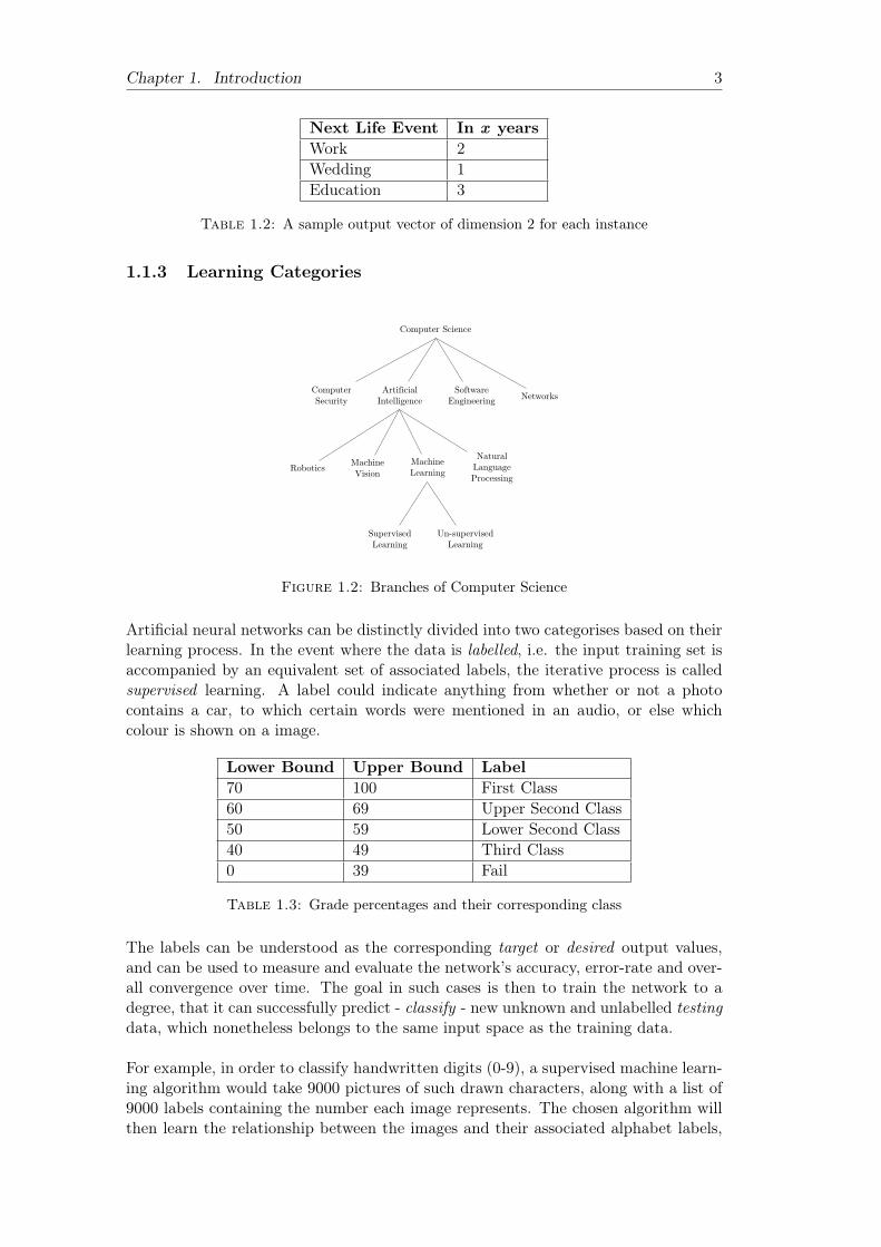
Next Life Event In x yearsWork 2Wedding 1Education 3

Table 1.2: A sample output vector of dimension 2 for each instance

1.1.3 Learning Categories

Computer Science

ComputerSecurity

ArtificialIntelligence

Robotics MachineVision

MachineLearning

SupervisedLearning

Un-supervisedLearning

NaturalLanguageProcessing

SoftwareEngineering Networks

Figure 1.2: Branches of Computer Science

Artificial neural networks can be distinctly divided into two categorises based on theirlearning process. In the event where the data is labelled, i.e. the input training set isaccompanied by an equivalent set of associated labels, the iterative process is calledsupervised learning. A label could indicate anything from whether or not a photocontains a car, to which certain words were mentioned in an audio, or else whichcolour is shown on a image.

Lower Bound Upper Bound Label70 100 First Class60 69 Upper Second Class50 59 Lower Second Class40 49 Third Class0 39 Fail

Table 1.3: Grade percentages and their corresponding class

The labels can be understood as the corresponding target or desired output values,and can be used to measure and evaluate the network’s accuracy, error-rate and over-all convergence over time. The goal in such cases is then to train the network to adegree, that it can successfully predict - classify - new unknown and unlabelled testingdata, which nonetheless belongs to the same input space as the training data.

For example, in order to classify handwritten digits (0-9), a supervised machine learn-ing algorithm would take 9000 pictures of such drawn characters, along with a list of9000 labels containing the number each image represents. The chosen algorithm willthen learn the relationship between the images and their associated alphabet labels,

Chapter 1. Introduction 4

and then apply that learned relationship to classify 1000 completely new unlabelledimages that it hasn’t seen before. If it manages to correctly classify 900 out of thetotal 1000 testing images, it would be said to have an accuracy of 90%, and an errorrate of 10%.

The other category, where the input data space is unknown and contains no asso-ciated labels, the process is called unsupervised learning. The goal is then not onlyto cluster the input data into groups, but also to discover the structure and patterns- the topology - of the input space itself, by grouping them into clusters according tothe similarity between one another.

Figure 1.3: Unsupervised learning clusters data solely according totheir feature similarities, as no labels are used

In contrast to supervised learning, we cannot directly measure the accuracy of thecalculated outputs because there are no target outputs to compare them with. Theperformance of the network is therefore often subjective and domain-specific. Theaccuracy of how well a network clusters data could depend on the effectiveness ofthe chosen algorithm, how well it is applied, and how much useful training data isavailable. An important feature of this type of learning is that no human interactionis needed. Indeed, as the model requires no labels, the human necessity to review thedata is bypassed, thus reducing by a considerable amount the time and effort requiredto assemble large datasets.

However, many datasets which can be used for unsupervised learning do come withlabels. These can simply be ignored if the aim is to study a particular unsupervisedlearning algorithm and its effectiveness. In this case, the labels can be used after thenetwork has finished training to measure the accuracy of the model, or simply aid inthe visualisation of the data after clustering.

An important property of neural networks is that a small portion of bad data ora small section of non-functional nodes will not cripple the entire network. It willinstead adapt, and continue working, unless the quantity of faulty data crosses theacceptable threshold, in which case incorrect outputs will be produced.

1.1.4 Learning Algorithms

Finally, the chosen algorithm is what determines two important elements: the archi-tecture and the eventual output of the network. The former is essentially the numberof layers, how nodes are linked to one another, and how the weight adjustments influ-ence other connected nodes. The output node is fired if the inputs exceed a certainthreshold.

These networks - supervised or unsupervised - can eventually become remarkably

Chapter 1. Introduction 5

capable of doing certain tasks that conventional programs cannot. Moreover, depend-ing on the task, the quantity and quality of the training data, the chosen algorithm,and the complexity and accuracy of a few other factors, the converged artificial neuralnetwork can match or even surpass surpass human ability at the task.

Machine LearningSupervised Unsupervised

Classification Regression Clustering DimensionalityReduction

Support VectorMachine (SVM)

Support VectorRegressor (SVR)

HebbianLearning

Principal ComponentAnalysis (PCA)

LogisticRegression

LinearRegression

Self OrganisingMaps (SOM)

Linear DiscriminantAnalysis (LDA)

NaiveBayes

DecisionTrees

MixtureModels

Flexible DiscriminantAnalysis (FDA)

NearestNeighbour (k-NN)

RandomForest k-Means Singular-Value

Decomposition (SVA)

Table 1.4: A few selected machine learning algorithms from the listedcategories.

One such type of neural network, Self-Organising Maps (SOM), and it’s learning algo-rithm by Kohonen Teuvo will be the focus of this study.

1.2 Problem

The problem this project attempts to solve is a mix of research, communication andimplementation tasks.

The principal problem of this project is the implementation of a Kohonen Networkas an application, in order to demonstrate its usefulness and explain the concepts ofMachine Learning, by means of a converging Self-Organising Map.

1.3 Aims

The aim of this project was to build a Kohonen network that is capable of clusteringdata, such as hand-drawn letters on an web program, and which would also allowusers to test their own data. The point of the of the web application, which hoststhe model, was to essentially act as an interactive learning tool for other interestedstudents or hobbyists on Machine Learning and Artificial Intelligence.

1.4 Objectives

1.4.1 Essential Features

• Implementing a fully functional Kohonen back-end model, capable of receivingand processing data from a chosen dataset.

• Training the network with a large quantity of data until it reaches a high accu-racy rate of clustering.

• Implementing a web application to host and interact with the developed model.

Chapter 1. Introduction 6

• The web application should communicate with the computational back-endmodel and retrieve the clusterisation data.

• Using different web pages for explanations of various concepts, features andparameters of the Kohonen algorithm in order to explain SOMs to users in lay-man’s terms.

• The website should have an interactive ‘Draw’ page where users can draw theirown letter on a Graphical User Interface (GUI) canvas and have the websiteprocess and display which letter it is, by interacting with the ANN model.

• The website should display the neural network’s topological map of alphabetsto the user based on training data.

• The website should have a page which displays animations or diagrams overtime of neural networks and SOMs, to show its evolution, how its weights areadjusted and converged, and how the network is trained over time.

• The website should have a ‘Database’ page which contains information on thedataset used to train and test the neural network, the size of the entire database,and links to the source-files.

• The website should have an ‘About’ page which contains information on tech-nologies, libraries, tools and algorithms used for building the project.

1.4.2 Desirable Features

• The website should highlight where your input would be placed on the displayedtopological map.

• The users should have an ‘in-depth’ option of seeing the steps the networkgoes through, such as re-centring, cropping and down-sampling of the input,probability numbers or graphs of which letter the input corresponds to.

• Allow users to input more than one single input at a time i.e. draw more thanone letter in the input canvas.

• The ‘database’ page, which should show a sample training data character foreach class, could also show the different handwritings for a specifically selectedalphabet. This is to give a visual representation and sense of scale of how manydifferent handwritten letters were used to train the neural network for eachalphabet.

• Some of the instructions sentences on the website could be written using thesynthetic training data images.

1.5 Predicted Challenges

Initially, the main predicted challenge was simply the implementation difficulty of theKohonen network model, and its visualisation on the front-end. Additionally, beingable to choose particularly relevant examples and methods to illustrate SOMs as ateaching tool were also considered as a potential challenge. Finally, the vast scopeand lack of real constraints were originally deemed problematic as well.

7

Chapter 2

Background

2.1 Problem

This problem is the implementation of a Kohonen model as a teaching tool for otherinterested students. It falls precisely into the category of pattern recognition in thefield of Machine Learning.

2.2 Existing Solutions

There have been a number of previous implementations of neural networks that at-tempt to cluster data, especially hand-written digits, due to the popularity of theMNIST dataset.

However, almost none of these models employ Kohonen’s algorithm for the task, asmany instead favour a supervised and error-correction learning by means of convolu-tional neural networks.

This project’s goal is not only to attempt to build a topological map of the inputdata, by using of an uncommon algorithm, but to do so with a much larger and com-plex dataset than the MNIST database. To add complexity to the task, alphabetsalong with digits were both used to build this implementation.

A model capable of distinguishing between similar digits and letters has certainlynot been developed, especially using with Kohonen’s learning process.

2.3 Research and Analysis

First of all, rigorous research went into conducting an extensive literature review on acompletely new topic, to understand the nature of Self-Organising Maps: their topo-logical mapping, competitive process, sample usages, general applications and actualimplementation. Furthermore, substantial work was done reviewing Dr Irina V. Bik-tasheva’s COMP305: Bio-computation module and Stanford’s excellent ‘Introductionto Machine Learning’ course by Prof. Andrew Ng. The results of this work can beseen in Chapter 2.

Secondly, research went into the system design and how to make the SOM interactivefor human users. All the extensive technologies, especially for front-end graphics vi-sualisation and back-end algorithmic modelling, were thoroughly examined, as heavydata visualisation was planned.

Chapter 2. Background 8

Lastly, publicly available datasets on handwritten input and existing similar appli-cations were examined in order to make a distinguished original project. There aremany existing real-time applications that use ANNs to classify hand-drawn digits usingthe MNIST dataset, but almost none that use a SOM with competitive learning to clusterhandwritten letters and display its topological map.

2.4 Project Requirements

This project firstly requires a user friendly front-end design, with interactive capa-bilities. HTML and CSS were both vital for this purpose. Secondly, a mathematicalback-end model with significant computing power was necessary to handle large quan-tities of data, and the task was best suited for Python and it’s libraries. Finally, tohost the topological map, JavaScript’s D3.js was perfect for this task as it requiredconsiderable data manipulation. More detailed use of technologies and programs aregiven in Chapter 5.

9

Chapter 3

Kohonen’s Self-Organising Maps

3.1 Background

Pioneered in 1982 by Finnish professor and researcher Dr. Teuvo Kohonen, a self-organising map is an unsupervised learning model, intended for applications in whichmaintaining a topology between input and output spaces is of importance. The no-table characteristic of this algorithm is that the input vectors that are close - similar- in high dimensional space are also mapped to nearby nodes in the 2D space. It is inessence a method for dimensionality reduction, as it maps high-dimension inputs to alow (typically two) dimensional discretised representation and conserves the underly-ing structure of its input space.

A valuable detail is that the entire learning occurs without supervision i.e. the nodesare self-organising. They are also called feature maps, as they are essentially retrain-ing the features of the input data, and simply grouping themselves according to thesimilarity between one another. This has a pragmatic value for visualising complexor large quantities of high dimensional data and representing the relationship betweenthem into a low, typically two-dimensional, field to see if the given unlabelled datahas any structure to it.

3.2 Structure

Figure 3.1: A Kohonen model

A SOM differs from typical ANNs both in its architecture and algorithmic properties.Firstly, its structure comprises of a single-layer linear 2D grid of neurons, instead of aseries of layers. All the nodes on this grid are connected directly to the input vector,but not to one another, meaning the nodes do not know the values of their neighbours,and only update the weight of their connections as a function of the given inputs. The

Chapter 3. Kohonen’s Self-Organising Maps 10

grid itself is the map that organises itself at each iteration as a function of the inputof the input data. As such, after clustering, each node has its own (i, j) coordinate,which allows one to calculate the Euclidean distance between 2 nodes by means of thePythagorean theorem.

(a) Rectangular (b) Hexagonal

Figure 3.2: Kohonen network’s nodes can be in a rectangular orhexagonal topology

3.3 Properties

A Self-Organising Map, additionally, uses competitive learning as opposed to error-correction learning, to adjust it weights. This means that only a single node is ac-tivated at each iteration in which the features of an instance of the input vector arepresented to the neural network, as all nodes compete for the right to respond to theinput. The chosen node - the Best Matching Unit (BMU) - is selected according tothe similarity, between the current input values and all the nodes in the grid. Thenode with the smallest Euclidean difference between the input vector and all nodesis chosen, along with its neighbouring nodes within a certain radius, to have theirposition slightly adjusted to match the input vector. By going through all the nodespresent on the grid, the entire grid eventually matches the complete input dataset,with similar nodes grouped together towards one area, and dissimilar ones separated.

Figure 3.3: A Kohonen model with the BMU in yellow, the layersinside the neighbourhood radius in pink and purple, and the nodes

outside in blue.

3.4 Variables

• t is the current iteration.

Chapter 3. Kohonen’s Self-Organising Maps 11

• n is the iteration limit, i.e. the total number of iterations the network canundergo.

• λ is the time constant, used to decay the radius and learning rate.

• i is the row coordinate of the nodes grid.

• j is the column coordinate of the nodes grid.

• d is the distance between a node and the BMU.

• ~w is the weight vector.

• wij(t) is the weight of the connection between the node i, j in the grid, and theinput vector’s instance at iteration t.

• ~x is the input vector.

• x(t) is the input vector’s instance at iteration t.

• α(t) is the learning rate, decreasing with time in the interval [0, 1], to ensurethe network converges.

• βij(t) is the neighbourhood function, monotonically decreasing and representinga node i, j’s distance from the BMU, and the influence it has on the learning atstep t.

• σ(t) is the radius of the neighbourhood function, which determines how farneighbour nodes are examined in the 2D grid when updating vectors. It isgradually reduced over time.

3.5 Algorithm

1. Initialise each node’s weight wij to a random value

2. Select a random input vector ~xk

3. Repeat following for all nodes in the map:

(a) Compute Euclidean distance between the input vector ~x(t) and the weightvector wij associated with the first node, where t, i, j = 0

(b) Track the node that produces the smallest distance d

4. Find the overall Best Matching Unit (BMU), i.e. the node with the smallestdistance from all calculated ones

5. Determine topological neighbourhood βij(t) its radius σ(t) of BMU in the KohonenMap

6. Repeat for all nodes in the BMU neighbourhood:

(a) Update the weight vector ~wij of the first node in the neighbourhood of theBMU by adding a fraction of the difference between the input vector ~x(t)and the weight ~w(t) of the neuron.

7. Repeat this whole iteration until reaching the chosen iteration limit t = n

Step 1 is the initialisation phase, while steps 2-7 represent the training phase.

Chapter 3. Kohonen’s Self-Organising Maps 12

3.6 Formulas

The updates and changes to the variables are done according to the following formulas:

The weights within the neighbourhood are updated as:

wij(t+ 1) = wij(t) + αi(t)[x(t)− wij(t)], or (3.1)wij(t+ 1) = wij(t) + αi(t)βij(t)[x(t)− wij(t)] (3.2)

The equation 3.1 tells us that the new updated weight wij(t + 1) for the node i, j isequal to the sum of old weight wij(t) and a fraction of the difference between the oldweight and the input vector x(t). In other words, the weight vector is ‘moved’ closertowards the input vector. Another important element to note is that the updatedweight will be proportional to the 2D distance between the nodes in the neighbour-hood radius and the BMU.

Furthermore, the same equation 3.1 does not account for the influence of the learn-ing being proportional to the distance a node is from the BMU. The updated weightshould take into factor that the effect of the learning is close to none at the extrem-ities of the neighbourhood, as the amount of learning should decrease with distance.Therefore, the equation 3.2 adds the extra neighbourhood function factor of βij(t),and is the more precise in-depth one.

σ(t)

βij

(t)

βij(t)

The radius and learning rate are both similarly and exponentially decayed with time:

σ(t) = σ0 · exp(−tλ

), where t = 1, 2, 3 . . . n (3.3)

α(t) = α0 · exp(−tλ

), where t = 1, 2, 3 . . . n (3.4)

The neighbourhood function’s influence βi(t) is calculated by:

βij(t) = exp (−d2

2σ2(t)), where t = 1, 2, 3 . . . n (3.5)

Chapter 3. Kohonen’s Self-Organising Maps 13

The Euclidean distance between each node’s weight vector and the current inputinstance is calculated by the Pythagorean formula:

||~x− ~wij || =

√√√√ n∑t=0

[~x(t)− ~wij(t)]2 (3.6)

The BMU is selected from all the node’s calculated distances as the one with thesmallest:

d = min(||~x− ~wij ||) = min(

√√√√ n∑t=0

[~x(t)− ~wij(t)]2) (3.7)

14

Chapter 4

Data

4.1 Data

The data in this chapter only refers to the training and/or testing datasets that wereused as inputs in the implemented Kohonen neural network in order to adjust itsweights and find an optimal output at each iteration. They do not refer to the 3rdparty feedback data explained in Chapter 10.

4.2 Ethical Use of Data

4.2.1 Real Non-Human and Synthetic Data

For the purpose of this project, only real non-human and synthetic data, specificallythe Iris, auto-generated RGB, and EMNIST dataset were used, and these were freelyavailable in the public domain. No human or any other type of data which requiresapproval from any professional ethical oversight body were ever utilised.

The Iris Flower dataset, created by biologist and statistician Ronald Fisher in 1936,is a published dataset containing a total of 150 training instances, each with fourmeasurements of sepal length, the sepal width, the petal length and the petal widthof the iris in question. There are 3 different iris classes, Iris setosa, Iris virginica andIris versicolor, and the dataset contains 50 samples of each. The data belongs toUniversity College Irvine’s Machine Learning Repository, which contains a collectionof databases that are often popular in Machine Learning communities. It representsreal non-human data, measured and collected out in the field.

The MNIST dataset, a subset of the NIST database, contains the data derived from60, 000 training and 10, 000 testing pictures of numerical handwritten digits by highschool students and employees of the United States Census Bureau. A character’sdata is set in a 28 by 28 pixel format, giving 784 total values between 0-255, eachone representing the grey scale intensity of that particular pixel. It is widely used forimage processing programs and networks.

The extended MNIST, or EMNIST dataset, follows the same format and conventions,but also contains data of upper and lower-case alphabets, along with the digits presentin the MNIST.

Both of these are in the public domain, and freely available in Matlab or binarydata format, which can be converted to .csv or .txt files. For this project, the datawas downloaded directly in .csv format from Kaggle, a popular Data Science and Ma-chine Learning platform website, recently acquired by Google.

Chapter 4. Data 15

Full references and samples of these datasets can be found in the Bibliography andAppendix B at the end of this document. A copy of the data was uploaded to myUniversity server, as a secure backup behind firewall.

4.2.2 Human Participation

For the realisation of this project, no human participation was involved, and thereforeno permissions or approvals were required. The program is based on data alreadypublicly available since many years, and only requires human interaction during theevaluation and usage phase, for which the consent form has been appended.

16

Chapter 5

Design

This chapter describes how the overall software and system was planned to work andinteract with all of it’s moving components, by giving an in depth explanation aboutthe flow of data.

5.1 Software Technologies

The following table lists out the technologies, languages, libraries and frameworksused to implement this project in its entirety.

Tasks Technologies Libraries

ImplementingKohonen SOM - Python

- NumPy- Pandas- Matplotlib- Argsparse

Training the networkwith synthetic data - Python

- Random RGB data- Iris Database- EMNIST Database

Implementing webapplication to host SOM

- HTML- CSS- JavaScript- Flask

- jQuery- AJAX- Bootstrap

Displaying topological mapand general model response - JavaScript - D3.js

Hosting and backingup source code - Github - Git

Hosting the websiteand model - Web server

- Localhost- University server- Github.io page

Table 5.1: Programming languages, technologies, and libraries usedfor different tasks in this project.

5.2 Data Structures

5.2.1 Logical Sequence

Training

The following is the sequence of events to train the neural net:

1. Input image

Chapter 5. Design 17

2. Feature Extraction and Preprocessing

3. Learning and Recognition using SOM:

(a) Initialise network

(b) Present input

(c) Best node wins via competitive learning

(d) Update weights accordingly

(e) Return winning node

4. Output result

5. Match output with labelled data

6. Output data

7. Repeat with different input

Figure 5.1

Testing

The following is the sequence of events to test the neural net:

1. Input image

2. Feature Extraction and Preprocessing

3. Recognition using SOM:

(a) Initialise network

(b) Present input

(c) Return winning node

4. Output result

5. Match output with labelled data

6. Output data

5.2.2 Image to Data Conversion

The EMNIST dataset contained images of handwritten characters, with each image be-ing 28x28 pixels. Similarly, the user’s input drawing had to be converted to a numericmatrix as well, based on the where the user had drawn on the canvas. A 1D vectorof 784 numbers was used to convert an image to a list of greyscale black and whitevalues in a 784-dimension array.

Chapter 5. Design 18

The following images show the planned sequence of image processing, to be imple-mented in a JavaScript front-end canvas, and its data transferred to the Pythonback-end.

(a) Empty grid (b) Character drawn on grid

(c) Pixelised grid(d) Corresponding matrix

Figure 5.2: Sample hand-drawn input character converted fromfront-end canvas stroke to individual pixel data values.

5.3 System Design

5.3.1 UML Class Diagram

Below is the original UML class diagram, employing HTML, CSS, JavaScript, andPython files to implement both ends of the project.

Chapter 5. Design 19

Figure 5.3: Use-Case Diagram

5.3.2 Use-case diagram

The following is a sample use-case diagram for the original user interface, which waslater slightly altered, rendering this diagram obsolete.

Chapter 5. Design 20

Figure 5.4: Use-Case Diagram

5.3.3 Use-case descriptions

The use-case descriptions for the given use-case diagram can be found in full in theAppendix E.

Chapter 5. Design 21

5.3.4 System boundary diagram

Below is the system boundary diagram for the both mobile and standard web users:

Figure 5.5: System boundary diagram

Chapter 5. Design 22

5.3.5 Sequence Diagram

The following is the sequence diagram when the user chooses the ‘draw’ option.

Figure 5.6: Sequence diagram for the drawing page

Chapter 5. Design 23

The sequence diagram can be broken down to the following detailed order of steps:

1. openWebsite(): user access the website

2. displayWebsite(): website content is displayed to user

3. chooseToDraw(): user chooses the ‘draw’ option button

4. displayCanvas(): website displays the drawable GUI canvas

5. draw(): user inputs on the canvas with his mouse or finger

6. displayStrokes(): website shows the strokes the user is drawing in real-time

7. finishDraw(): user submits his drawing

8. sendDrawingData(): website sends the drawing data’s pixel values to the com-putational model as an array of integers or doubles

9. stopCanvas(): website stops displaying a drawable canvas to the user

10. inputsData(): model is fed the user’s drawn data array

11. bestMatchingUnit(): computational model finds the best matching unit

12. returnLetter(): model returns the highest similarity letter’s index

13. displayResize(): website shows the user the re-centring and re-sizing of his draw-ing

14. displaySampling(): website down-samples the user input drawing

15. displayLetter(): the corresponding letter with the highest similarity to the inputdrawing is displayed to the user

16. makeMap(): the topological map’s data are arranged in arrays to be shown

17. displayMap(): the map is shown to the user using front-end graphics and thedata from the array

18. placeInputLetterOnMap(): calculate where the user input would be placed onthe map by sorting it in the array containing the other value points

19. displayInputLetterOnMap(): user’s input letter is shown where it would belongon the map

20. closeWebsite(): user closes the website

21. shutDown(): the web application shuts down

Chapter 5. Design 24

The following is the sequence diagram when the user chooses the ‘learn’ option.

Figure 5.7: Sequence diagram for the learning page

Chapter 5. Design 25

The sequence diagram can be broken down to the detailed order of steps:

1. openWebsite(): user access the website

2. displayWebsite(): website content is displayed to user

3. chooseToLearn(): user chooses the ‘learn’ option button

4. displayLearningPage(): website displays ‘learn’ page

5. clickAnimation(): user presses play on an animation

6. playAnimation(): website plays the animation

7. clickMap(): user requests to open or see the topological map of the training setdata

8. requestMap(): website requests the map from the computational model

9. computeMap(): computational model computes the map

10. returnData(): computational model returns the data of the map in a hash

11. buildMap(): website builds the map using the hash and its data

12. displayMap(): website displays the map to the user

13. hoverOnMapPoint(): user hovers on a specific map point

14. getMapPointLabel(): data for that specific point is fetched in the hash using thekey

15. displayLabel(): data for that specific point is displayed

16. closeWebsite(): user closes the website

17. shutDown(): the web application shuts down

The sequence diagrams attempt to illustrate the interaction between user(s) and thepages via the computational model, and the flow of events as they happen.

5.4 Algorithm Design

The next few sub-sections contain key examples of pseudo-code and on how the in-teraction between components was planned.

5.4.1 Self-Organising Map

The Self-Organising Map is to be generated by the python computational model atthe back end, which adjusts the network’s weights during training with synthetic dataand cluster similar inputs together.

1. Setup

(a) Import necessary libraries

(b) Create virtual environment

(c) Create required dataframe to contain input values

(d) Choose parameters: SOM size, learning parameters

(e) Create grid

2. Normalisation

(a) Normalise input data vectors

Chapter 5. Design 26

• RGB: 3 vectors with values from 0 to 255.• Greyscale: single vector with values will be from 0 to 255.• Black and white: binary 0 or 1 values.

3. Learning

(a) Initilise nodes’ weights to random values

(b) Select Random Input Vector

(c) Repeat following for all nodes in the map:

i. Compute Euclidian Distance between the input vector and the weightvector associated with the first node

ii. Track the node that produces the smallest distance

(d) Find the overall Best Matching Unit (BMU), i.e. the one with the smallestdistance of all the nodes

(e) Determine topological neighbourhood of BMU in the Kohonen Map

(f) Repeat for all nodes in the BMU neighbourhood:

i. Update the weight vector of the first node in the neighbourhood of theBMU by adding a fraction of the difference between the input vector andthe weight of the neuron

(g) Repeat this whole iteration until reaching the chosen iteration limit

4. Visualisation

(a) Make use of Matplotlib for development, local testing and visualisation

(b) Final visualisation for the user was to be done by the front end with D3.js

Chapter 5. Design 27

5.4.2 Canvas

The canvas on the front-end is the graphical user interface the user sees as the inputarea in which to draw his letter using a pointing devices such as a mouse, or by handon a touch screen device. To achieve this, the canvas must have 4 event listeners forthe mouse and then draw black pixels continuously along where the user inputs datain the correct events. The pseudo-code for the events can be summarised as shownbelow.

Algorithm 1 Mouse Move Eventif mouseMove thendrawable ← truegetCoordinates()

end if

Algorithm 2 Mouse Down Eventif mouseDown thendrawable ← falsegetCoordinates()

end if

Algorithm 3 Mouse Up Eventif mouseUp thendrawable ← false

end if

Algorithm 4 Mouse Out Eventif mouseOut thendrawable ← false

end if

Algorithm 5 getCoordinates() FunctionPreviousX ← CurrentXPreviousY ← CurrentYCurrentX ← EventX−canvas.offsetLeftCurrentY ← EventY−canvas.offsetTopif drawable ← true thendraw()

end if

Chapter 5. Design 28

Algorithm 6 draw() Function

canvas.beginPath()canvas.moveTo(PreviousX ,PreviousY )canvas.lineTo(CurrentX ,CurrentY )canvas.drawLine(CurrentX ,CurrentY )canvas.stroke()canvas.closePath()

Where:

• mouseDown is an event where the user only touches the screen, but does notyet draw, meaning only the fixed input coordinates are required.

• mouseMove is an event where the user draws on the screen, thereby continuouslycalling the draw function as the input position varies.

• mouseUp is an event where the user stops inputting.

• mouseOut is an event where the user leaves the canvas drawable area.

• getCoordinates and draw() are methods.

• drawable is a boolean

• offsetLeft is an HTMLcanvas property that returns ‘the number of pixels thatthe upper left corner of the current element is offset to the left within theHTMLElement.offsetParent node’.

• offsetLeft is an HTMLcanvas property that returns ‘the distance of the currentelement relative to the top of the offsetParent node’.

• PreviousX , PreviousY , CurrentX , CurrentY are ints about the input coordi-nates via the mouse or finger.

• beginPath(), moveTo(), lineTo(), drawLine(), closePath() are all HTML methodsthat reference the canvas tag.

29

Chapter 6

Front-End

6.1 Realisation

This chapter presents a comprehensive and in-depth review of how each section ofthe entire project, and its many components, were implemented in the chronologicalorder, coupled with the obstacles and their respective solutions encountered duringthe realisation. Each part’s design, structure and technical aspects are thoroughlyexamined and their net utility assessed.

The front-end was the first section to be implemented, with the HTML, CSS, JavaScriptall developed more or less simultaneously, requiring a substantial mix of various li-braries, tools, and an abundant amount of adjustments. The aesthetics of a websiteis a prominent part of its look and feel, and was thus carefully considered and andconstructed as described below.

6.2 Bootstrap

6.2.1 Review

The Bootstrap documentation was formally reviewed to consider all the possible com-ponents such as navigation bars, footers, and headers, which could serve a purpose aspart of the website and add to the UI/UX, without feeling contrived. This took prece-dence over writing the HTML, as a clear idea of what tools and objects were beingused from the ground up was required before building the system, as any changes at alater stage would only be detrimental. The fact that newer versions of Bootstrap arecontinuously being released needed to be kept in mind. This project was specificallybuilt using Bootstrap v4.0.0.

6.2.2 Integration

Adding the Bootstrap framework onto a project can be done in several ways. A pack-age manager such as npm, Bundler, RubyGems, or Composer can be used to downloadand compile the source files. Alternatively, the compiled or source files, which containthe the minified CSS bundles and JavaScript plug-ins, can be manually downloadedand dropped into the project’s directory. However, both approaches require meticu-lousness. Messy file management can simply be avoided by having the pre-compiledand cached version of Bootstrap’s CSS and JS downloaded directly into the projectas the index file is loaded.

Chapter 6. Front-End 30

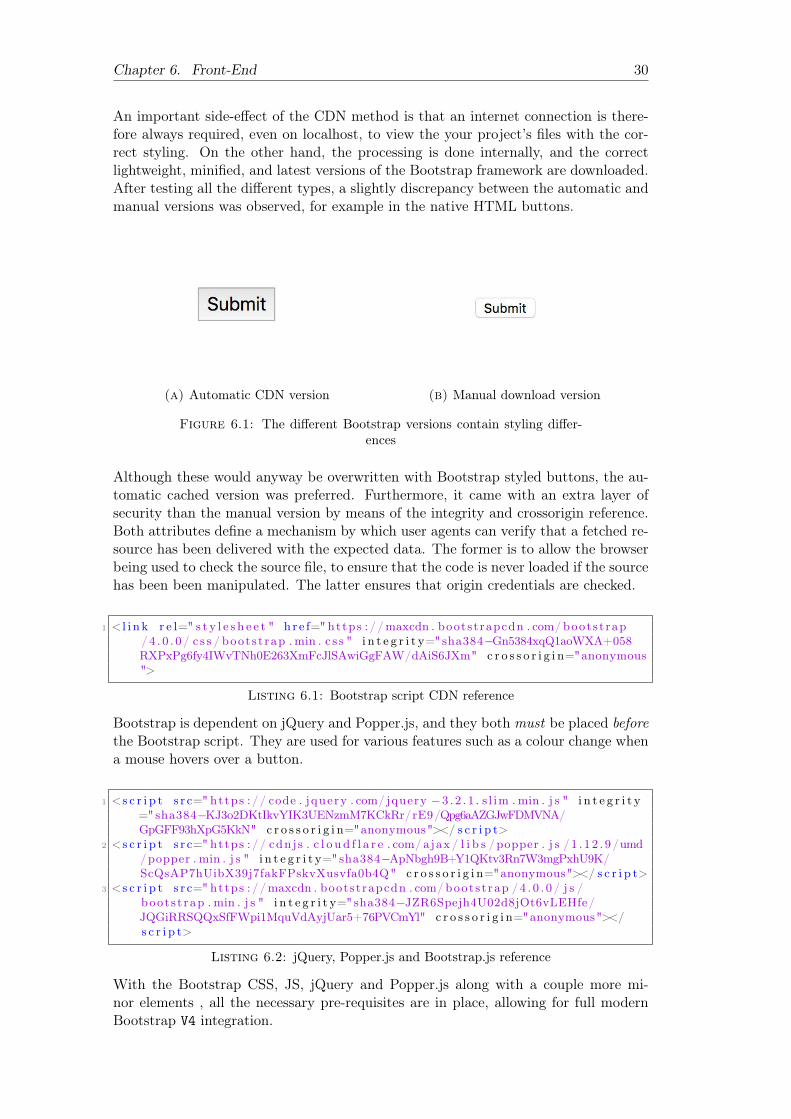
An important side-effect of the CDN method is that an internet connection is there-fore always required, even on localhost, to view the your project’s files with the cor-rect styling. On the other hand, the processing is done internally, and the correctlightweight, minified, and latest versions of the Bootstrap framework are downloaded.After testing all the different types, a slightly discrepancy between the automatic andmanual versions was observed, for example in the native HTML buttons.

(a) Automatic CDN version (b) Manual download version

Figure 6.1: The different Bootstrap versions contain styling differ-ences

Although these would anyway be overwritten with Bootstrap styled buttons, the au-tomatic cached version was preferred. Furthermore, it came with an extra layer ofsecurity than the manual version by means of the integrity and crossorigin reference.Both attributes define a mechanism by which user agents can verify that a fetched re-source has been delivered with the expected data. The former is to allow the browserbeing used to check the source file, to ensure that the code is never loaded if the sourcehas been been manipulated. The latter ensures that origin credentials are checked.

1 <l i n k r e l=" s t y l e s h e e t " h r e f=" https : //maxcdn . bootstrapcdn . com/ bootst rap/4 . 0 . 0 / c s s / boots t rap . min . c s s " i n t e g r i t y="sha384−Gn5384xqQ1aoWXA+058RXPxPg6fy4IWvTNh0E263XmFcJlSAwiGgFAW/dAiS6JXm" c r o s s o r i g i n="anonymous">

Listing 6.1: Bootstrap script CDN reference

Bootstrap is dependent on jQuery and Popper.js, and they both must be placed beforethe Bootstrap script. They are used for various features such as a colour change whena mouse hovers over a button.

1 <s c r i p t s r c=" https : // code . jquery . com/ jquery −3 . 2 . 1 . s l im . min . j s " i n t e g r i t y="sha384−KJ3o2DKtIkvYIK3UENzmM7KCkRr/rE9/Qpg6aAZGJwFDMVNA/GpGFF93hXpG5KkN" c r o s s o r i g i n="anonymous"></ s c r i p t>

2 <s c r i p t s r c=" https : // cdnj s . c l o u d f l a r e . com/ ajax / l i b s /popper . j s /1 . 12 . 9/umd/popper . min . j s " i n t e g r i t y="sha384−ApNbgh9B+Y1QKtv3Rn7W3mgPxhU9K/ScQsAP7hUibX39j7fakFPskvXusvfa0b4Q" c r o s s o r i g i n="anonymous"></ s c r i p t>

3 <s c r i p t s r c=" https : //maxcdn . bootstrapcdn . com/ boots t rap /4 . 0 . 0 / j s /boots t rap . min . j s " i n t e g r i t y="sha384−JZR6Spejh4U02d8jOt6vLEHfe/JQGiRRSQQxSfFWpi1MquVdAyjUar5+76PVCmYl" c r o s s o r i g i n="anonymous"></s c r i p t>

Listing 6.2: jQuery, Popper.js and Bootstrap.js reference

With the Bootstrap CSS, JS, jQuery and Popper.js along with a couple more mi-nor elements , all the necessary pre-requisites are in place, allowing for full modernBootstrap V4 integration.

Chapter 6. Front-End 31

6.2.3 Colour Theme

The first task was to fully define the look and feel of the web-application which islargely contingent on the selected colour theme and font. A peachy, light colouredbackground (#fff2e7) was instinctively chosen for it’s soothing effect on the eyes.For all the other DOM objects, Bootstrap’s limited handful of colours1 were bold andcomplementary to both the background and one another. Attractive and user-friendly,they also maintained consistency across all pages. This was preferable over manuallyhand-picking a colour for a new item every time. More importantly, they nativelyworked for all Bootstrap components, simply by adding the colour tag to the DOMobject’s class names.

Figure 6.2: A handful of strong colour options provided natively inthe Bootstrap framework and their corresponding class names

A paragraph could simply be:

1 <p c l a s s="chosen−c l a s s−name text−i n f o ">Blue paragraph , with a <a hr e f="l i n k . html" c l a s s=" text−danger ">red l i n k</a></p>

Listing 6.3: Class colour code

And it would produce the following output on an HTML page with two distinctcolours:

Figure 6.3: Output

The point being that the colouring works despite the fact that there are two classnames. Bootstrap’s colour name tags can simply be appended to the class indepen-dently named by the developer, allowing further styling modifications in the CSS file.The modular streamlined nature of Bootstrap and its lack of dependencies is whatmakes it easy to grasp and work with.

6.2.4 Header

A fixed position navigation bar2 containing the website title throughout all pages wasindispensable to maintain consistency and a reference. A ‘Home’ and ‘About’ buttonwere added to the fringes of the navbar as well. The title evolved from a lengthy Ko-honen Self-Organising Maps: Pattern Recognition and Clustering from the EMNIST

1Bootstrap Getting Started. https://getbootstrap.com/docs/4.0/getting-started/theming/#theme-colors. (Accessed on 04/02/2018).

2Bootstrap Navbar. https://getbootstrap.com/docs/4.0/components/navbar/. (Accessed on04/02/2018).

Chapter 6. Front-End 32

database over several vertical lines to a simple Kohonen Self-Organising Maps.

1 <nav c l a s s="navbar f ixed−top bg−su c c e s s ">2 <a c l a s s="order−1 nav−item nav−l i n k a c t i v e " a s t y l e=" co l o r : white " h r e f

="/">Home</a>3 <a c l a s s="order−2 a l i gn−s e l f −cente r nav−item" a s t y l e=" co l o r : white "><b

>Kohonen Se l f−Organis ing Maps</b></a>4 <a c l a s s="order−3 nav−item nav−l i n k " a s t y l e=" co l o r : white " h r e f="about

">About</a>5 </nav>

Listing 6.4: Header code

Figure 6.4: Header evolution from prototype to final implementation

6.2.5 Footer

Originally, a two part footer was envisioned to be put in a fixed position for all pages,similar to the navbar, containing a line on the aim of the website coupled with thewebsite developer’s name. This was disregarded early on for taking up too much screensize, and a smaller single footer was used for a large part of the development beforebeing discarded too. The footer was pointless if it didn’t contain any new informationrelevant to each page.

Thus, the choice was between having a pagination or progress bar. The former wasfirst implemented and tested, but eventually disposed off as its white background didnot fit into the colour scheme, and the total number of pages was not known yet.Instead, a thin, slick and dynamic progress bar was developed which was consistentwith the colour scheme. It has all five colours, one for each section, and progressivelyfills each one out until reaching the last web-page.

1 <div c l a s s=" f o o t e r ">2 <div c l a s s=" f ixed−bottom">3 <div c l a s s=" prog r e s s ">4 <div c l a s s=" progres s−bar" r o l e=" progre s sbar " s t y l e="width : 20%"

ar ia−valuenow="15" ar ia−valuemin="0" ar ia−valuemax="100"></div>5 <div c l a s s=" progres s−bar bg−su c c e s s " r o l e=" progre s sba r " s t y l e="

width : 20%" ar ia−valuenow="30" ar ia−valuemin="0" ar ia−valuemax="100"></div>

6 <div c l a s s=" progres s−bar bg−i n f o " r o l e=" progre s sba r " s t y l e="width :20%" ar ia−valuenow="20" ar ia−valuemin="0" ar ia−valuemax="100"></div>

Chapter 6. Front-End 33

7 <div c l a s s=" progres s−bar bg−warning" r o l e=" progre s sbar " s t y l e="width : 10%" ar ia−valuenow="25" ar ia−valuemin="0" ar ia−valuemax="100"></div>

8 <div c l a s s=" progres s−bar bg−danger " r o l e=" progre s sbar " s t y l e="width : 0%" ar ia−valuenow="15" ar ia−valuemin="0" ar ia−valuemax="100"></div>

9 </div>10 </div>11 </div>

Listing 6.5: Footer code

Figure 6.5: Footer

6.2.6 Flex

On top of being dynamic, it was equally important that all the web-pages be flexi-ble, as modern screens come in all shapes and sizes. One of Bootstrap v4’s crowningfeatures was utilised: flex3 . This made sure the header and footer were responsiveto a certain degree to the width of the page, depending on the user’s screen size andresolution.

1 <div c l a s s="d−sm−f l e x f l e x−wrap f ixed−top">2 <nav c l a s s="navbar f ixed−top bg−su c c e s s ">3 . . .4 </nav>5 </div>

Listing 6.6: Flex code

Figure 6.6: Header with flex implementation

6.2.7 Columns

One of Bootstrap’s foundational feature is its columns grid structure4 based on flexbox.It allows for responsive design directly in each separate class. Essentially a page’s mainarea can be broken down into columns of a preferred size, allowing for easy manipu-lation and alignment of inline DOM objects.

1 <div c l a s s=" col−lg−12">2 . . .3 </div>

Listing 6.7: Column code

3Bootstrap Flex. https://getbootstrap.com/docs/4.0/utilities/flex/. (Accessed on04/02/2018).

4Bootstrap Columns Grid Layout. https://getbootstrap.com/docs/4.0/layout/grid/. (Ac-cessed on 04/02/2018).

Chapter 6. Front-End 34

There is also a very useful option where the columns are offset by a chosen columnsize.

1 <div c l a s s=" col−lg−8 o f f s e t−lg−2">2 . . .3 </div>

Listing 6.8: Offset column code

6.2.8 Buttons

Bootstrap offers straightforward buttons5 in various sizes, all of which can be colouredin any of the aforementioned tints. Small and normal sizes were used according totheir importance and the available space in that particular context.

1 <button type="button" c l a s s="btn btn−l g "><a hr e f="#">Button T i t l e</a></button>

Listing 6.9: Buttons code

6.2.9 Cards

Cards6 were flexible content containers perfect for proposing the user with options.Each one of them was used for one of the three datasets, highlighting each one’s fea-tures regarding their dimensionality and volume. Once again, different colours wereemployed to maintain colour scheme and distinguish one from the other by supposed‘difficulty’.

1 <div c l a s s="card−deck">2 <div c l a s s=" card text−white bg−i n f o mb−3" s t y l e="width : #px ; ">3 <img c l a s s="card−img−top" s r c="#" a l t="##">4 <div c l a s s="card−body">5 <h5 c l a s s="card−t i t l e ">Card T i t l e</h5>6 <p c l a s s="card−t ex t "></p>7 <a hr e f="#" c l a s s="card−l i n k "> . . .</a>8 </div>9 <div c l a s s="card−f o o t e r ">

10 . . .11 </div>12 </div>13 </div>

Listing 6.10: Single card code

6.2.10 jQuery

The jQuery integrated at the set-up phase with the crossorigin and integrity layer wasthe slim version7, which is a streamlined and shortened version of the full jQuery. As

5Bootstrap Buttons. https://getbootstrap.com/docs/4.0/components/buttons/. (Accessedon 04/02/2018).

6Bootstrap Cards. https://getbootstrap.com/docs/4.0/components/card/. (Accessed on04/02/2018).

7Bootstrap jQuery. https://getbootstrap.com/docs/4.0/getting-started/download/#bootstrapcdn. (Accessed on 04/02/2018).

Chapter 6. Front-End 35

it was revealed after intense debugging, this version is incompatible with Ajax andwas the cause of several mysterious bugs. Therefore, in some pages it was replacedwith the full version jQuery instead, at the expense of the aforementioned extra coverof security.

6.3 HTML

Once sufficient knowledge was gathered through research on the tools and components,and correctly integrated onto the foundations of the website, the main structure andcontent of each page had to be filled as an .html file. This was, like many other parts,a continuous iterative process, evolving till the very end. Thus, it was important tospend time designing a satisfactory template which could be used as a basis for allpages.

6.3.1 Template

The template consisted of bringing together all the previously researched elements,such as the background, buttons, cards, nav bar and progress bar, onto a single flexi-ble page built with the columns layout structure and flexbox. Additionally, the minorbut obligatory touches for a HTML5 page were also required. This encompassed themeta-information (such as the charset, and author’s name, date, ID), the cloud boot-strap and then the personal CSS files reference, the favicons themselves, and finallythe page’s title just in the file’s header section.

1 <head>2 <!−− META −−>3 <meta cha r s e t="UTF−8"/>4 <meta name="author " content=" . . . ">5 <meta name="ID" content=" . . . ">6 <meta name="Date" content="2018−02−25" scheme="YYYY−MM−DD">7 <meta name="viewport " content="width=device−width , i n i t i a l −s c a l e =1,

shr ink−to− f i t=no">8

9 <!−− Cloud Bootstrap CSS −−>10 <l i n k r e l=" s t y l e s h e e t " h r e f=" https : //maxcdn . bootstrapcdn . com/ bootst rap

/4 . 0 . 0 / c s s / boots t rap . min . c s s " i n t e g r i t y="sha384−Gn5384xqQ1aoWXA+058RXPxPg6fy4IWvTNh0E263XmFcJlSAwiGgFAW/dAiS6JXm" c r o s s o r i g i n="anonymous">

11

12 <!−− Main CSS −−>13 <l i n k h r e f=" s t a t i c / c s s /main . c s s " r e l=" s t y l e s h e e t " type=" text / c s s ">14

15 <!−− Favicons −−>16 <l i n k r e l=" . . . " s i z e s=" . . . " h r e f=" . . . ">17

18 <t i t l e> . . .</ t i t l e>19 </head>

Listing 6.11: HTML header code

The structure of the main body consisted first and foremost of a JavaScript onload()function in the HTML body declaration tag itself, followed by the nav bar, maincontent container, footer, and lastly a list of JavaScript declarations in the correctorder. All script lists contained a <noscript> error message in case the user did nothave JavaScript enabled, and were then followed by any personally developed scripts,before ending with the mandatory 3rd party jQuery, Popper.js and Bootstrap.js code

Chapter 6. Front-End 36

required for Bootstrap v4.

1 <body onload="setUp ( ) ; ">2

3 <!−− Nav bar −−>4 <div c l a s s="d−sm−f l e x f l e x−wrap f ixed−top">5 <nav c l a s s="navbar f ixed−top bg−su c c e s s ">6 . . .7 </nav>8 </div>9

10 <!−− Main −−>11 <div c l a s s="main">12 <div c l a s s=" col−lg−8 o f f s e t−lg−2">13 . . .14 </div>15 </div>16

17 <!−− Footer −−>18 <div c l a s s=" f o o t e r ">19 <div c l a s s=" f ixed−bottom">20 <div c l a s s=" prog r e s s ">21 . . .22 </div>23 </div>24 </div>25

26 <!−− Sc r i p t s −−>27 <nos c r i p t>Your browser does not support JavaScr ipt which i s r equ i r ed

by Bootstrap 4 f o r the purposes o f t h i s wep−page .</ no s c r i p t>28

29 <!−− Persona l S c r i p t s −−>30 <s c r i p t s r c=" . . . " type=" text / j a v a s c r i p t " cha r s e t="UTF−8"></ s c r i p t>31

32 <!−− jQuery −−>33 <s c r i p t s r c=" https : // code . jquery . com/ jquery −3 . 2 . 1 . s l im . min . j s "

i n t e g r i t y="sha384−KJ3o2DKtIkvYIK3UENzmM7KCkRr/rE9/Qpg6aAZGJwFDMVNA/GpGFF93hXpG5KkN" c r o s s o r i g i n="anonymous"></ s c r i p t>

34

35 <!−− Popper . j s −−>36 <s c r i p t s r c=" https : // cdnj s . c l o u d f l a r e . com/ ajax / l i b s /popper . j s /1 . 12 . 9/

umd/popper . min . j s " i n t e g r i t y="sha384−ApNbgh9B+Y1QKtv3Rn7W3mgPxhU9K/ScQsAP7hUibX39j7fakFPskvXusvfa0b4Q" c r o s s o r i g i n="anonymous"></ s c r i p t>

37

38 <!−− Boostrap . j s −−>39 <s c r i p t s r c=" https : //maxcdn . bootstrapcdn . com/ boots t rap /4 . 0 . 0 / j s /

boots t rap . min . j s " i n t e g r i t y="sha384−JZR6Spejh4U02d8jOt6vLEHfe/JQGiRRSQQxSfFWpi1MquVdAyjUar5+76PVCmYl" c r o s s o r i g i n="anonymous"></s c r i p t>

40 </body>

Listing 6.12: HTML body code

Lastly, the whole head and body content should of course be enclosed in the standardhtml declaration tag.

1 <! doctype html>2 <html lang="en">3 <head>4 . . .5 </head>

Chapter 6. Front-End 37

6 <body>7 . . .8 </body>9 </html>

Listing 6.13: HTML declarations

This was the designed framework used by all subsequent pages.

Figure 6.7: Front page template containing Bootstrap based navbar, column grid layout, main text container, button, progress bar

and general colour theme.

6.4 Art

In order to add a personal aspect to the website, hand-drawn art was added to thewebsite to complement the digital features. These were drawn with a stylus on aWacom tablet8 linked directly to Adobe Photoshop, and exported with a .png image.These can be found in full size in Appendix C at the end of this document.

6.4.1 Background Nets

As the background felt too bare simply as a monotone colour, an artistic renderingof neural networks was designed to add more focus towards the centred text. Theoriginal prototype contained black outlines for each node, which took away attentionfrom the text, and was subsequently altered to a version with grey outlined nodes. Theimage colour was also switched from white to the one used for the original backgroundimage, as the former would go on top of the latter.

8Wacom Intuos Pro-Medium Paper Edition Tablet

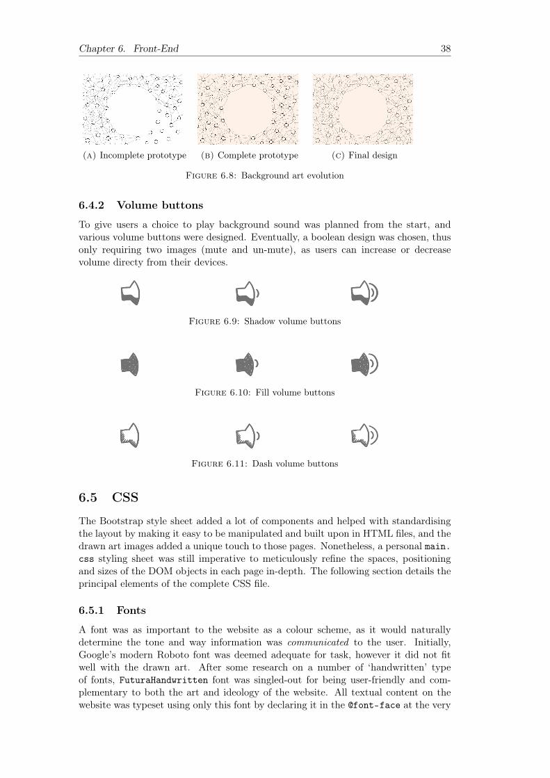
Chapter 6. Front-End 38

(a) Incomplete prototype (b) Complete prototype (c) Final design

Figure 6.8: Background art evolution

6.4.2 Volume buttons

To give users a choice to play background sound was planned from the start, andvarious volume buttons were designed. Eventually, a boolean design was chosen, thusonly requiring two images (mute and un-mute), as users can increase or decreasevolume directy from their devices.

Figure 6.9: Shadow volume buttons

Figure 6.10: Fill volume buttons

Figure 6.11: Dash volume buttons

6.5 CSS

The Bootstrap style sheet added a lot of components and helped with standardisingthe layout by making it easy to be manipulated and built upon in HTML files, and thedrawn art images added a unique touch to those pages. Nonetheless, a personal main.css styling sheet was still imperative to meticulously refine the spaces, positioningand sizes of the DOM objects in each page in-depth. The following section details theprincipal elements of the complete CSS file.

6.5.1 Fonts

A font was as important to the website as a colour scheme, as it would naturallydetermine the tone and way information was communicated to the user. Initially,Google’s modern Roboto font was deemed adequate for task, however it did not fitwell with the drawn art. After some research on a number of ‘handwritten’ typeof fonts, FuturaHandwritten font was singled-out for being user-friendly and com-plementary to both the art and ideology of the website. All textual content on thewebsite was typeset using only this font by declaring it in the @font-face at the very

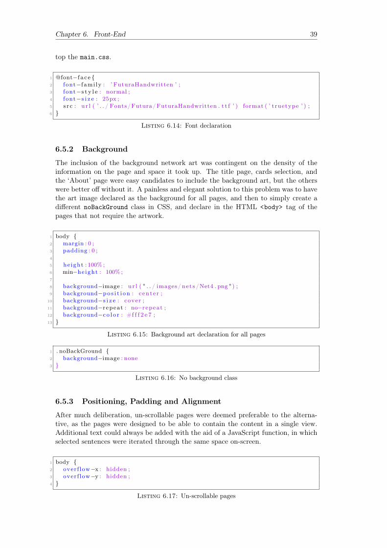
Chapter 6. Front-End 39

top the main.css.

1 @font−f a c e {2 font−f ami ly : ’ FuturaHandwritten ’ ;3 font−s t y l e : normal ;4 font−s i z e : 25px ;5 s r c : u r l ( ’ . . / Fonts/Futura/FuturaHandwritten . t t f ’ ) format ( ’ truetype ’ ) ;6 }

Listing 6.14: Font declaration

6.5.2 Background

The inclusion of the background network art was contingent on the density of theinformation on the page and space it took up. The title page, cards selection, andthe ‘About’ page were easy candidates to include the background art, but the otherswere better off without it. A painless and elegant solution to this problem was to havethe art image declared as the background for all pages, and then to simply create adifferent noBackGround class in CSS, and declare in the HTML <body> tag of thepages that not require the artwork.

1 body {2 margin : 0 ;3 padding : 0 ;4

5 he ight : 100% ;6 min−he ight : 100% ;7

8 background−image : u r l ( " . . / images / nets /Net4 . png ") ;9 background−po s i t i o n : c en t e r ;

10 background−s i z e : cover ;11 background−repeat : no−repeat ;12 background−c o l o r : #f f f 2 e 7 ;13 }

Listing 6.15: Background art declaration for all pages

1 . noBackGround {2 background−image : none3 }

Listing 6.16: No background class

6.5.3 Positioning, Padding and Alignment

After much deliberation, un-scrollable pages were deemed preferable to the alterna-tive, as the pages were designed to be able to contain the content in a single view.Additional text could always be added with the aid of a JavaScript function, in whichselected sentences were iterated through the same space on-screen.

1 body {2 over f low−x : hidden ;3 over f low−y : hidden ;4 }

Listing 6.17: Un-scrollable pages

Chapter 6. Front-End 40

Moreover, this allowed for easier manipulation of the header and footer. Both neededto stay in their place and never move regardless of the user interaction. The headerwas made sure to start from completely on top and be in its natural position, whilefooter’s position was made absolute and without any content below it.

1 . header {2 top : 0 ;3 width : 100% ;4 }

Listing 6.18: Header position

1 . f o o t e r {2 po s i t i o n : abso lu t e ;3 bottom : 0 ;4 width : 100% ;5 }

Listing 6.19: Footer position

Practically each DOM object was almost always given a certain amount of paddingon all 4 sides, and its text aligned centrally.

1 . ob j e c tC l a s s {2 padding−top : 20px ;3 padding−bottom : 20px ;4 padding− l e f t : 20px ;5 padding−r i g h t : 20px ;6 text−a l i g n : l e f t ;7 }

Listing 6.20: Sample object padding and alignment

Figure 6.12: Cover page with art, Bootstrap and personal CSS

Chapter 6. Front-End 41

6.6 JavaScript

Finally, the JavaScript is what makes the page interactive with the users, and distin-guishes the website from a fancy but passive booklet or sideshow. Several differentscripts were used and are outlined below.

6.6.1 Draw.js

Draw.js was a personal script used to initialise various variables on every page, andadd user interactivity. It’s principal focus was the development of the canvas usableby a user to input his own hand-drawn character.

The canvas was initialised in the setUpCanvas() function, which would get the can-vas’s initial values from the HTML page.

1 i n f o = document . getElementById ( ’status’ ) ;2 canvas = document . getElementById ( ’myCanvas’ ) ;3 ctx = canvas . getContext ( ’2d’ ) ;4 l en = canvas . width ;

Listing 6.21: Canvas Code

Simultaneously it would also call four other 3 main canvas drawing functions, corre-sponding to the ones detailed in Section 5.4.2.

1 // Calls2 setUpMouseCanvas ( ) ;3 setUpTouchCanvas ( ) ;4 se tUpScro l lEvents ( ) ;

Listing 6.22: Canvas event functions

Each one of these functions allow the user to draw inputs with a mouse or even ona mobile device using a touchscreen. For such cases it was important to disable autoscroll when the user would start inputting his data. Boolean values were used todecide when the could or couldn’t draw in the canvas.

1 // Prevent unintended touch scroll2 document . body . addEventListener ("touchstart" , function ( e ) {3 i f ( e . t a r g e t == canvas ) {4 e . preventDefau l t ( ) ;5 }6 } , fa l se ) ;

Listing 6.23: Disable auto-scroll on touch devices

A mysterious issue here was a random offsetting on the X-axis of the drawn lines.Indeed, everytime a line was attempted to be drawn on the canvas, it would appear afew centimers to the left, often not visible on the canvas. This was later identified tobe caused by Bootstrap’s grid layout structure, in which offset-columns were used.To disentangle this issue jQuery’s this.offset methods proved to be useful.

1 var o f f s e t L = this . o f f s e t L e f t + $ ( this ) . parent ( ) . o f f s e t ( ) . l e f t − 15 ;2 var o f f s e tT = this . o f f s e tTop + $ ( this ) . parent ( ) . o f f s e t ( ) . top ;

Listing 6.24: Correcting Bootstrap column’s offset on the canvas

Chapter 6. Front-End 42

A simple way to clear the canvas when required was to draw a rectangle of the canvas’ssize on it everytime the relevant requesting button was pressed. However, an evensmarter solution was implemented, which re-initialised the canvas’ height and width,thus removing any drawn strokes.

1 canvasIndImage . width = canvasIndImage . width ;

Listing 6.25: Clearing canvas

The bulk of the work went into developing a system which could intake more than asingle input drawn in the canvas. This was perhaps a bit ambitious and not reallynecessary, but was taken on as a challenge early on nonetheless.

The first step was to get the user’s entire data from the entire canvas. Then, eachindividual digit drawn in the canvas could be attempted to be seperated by iteratingrow-by-row through all the pixels containing any greyscale value. By adding eachgreyscale value which is continous or adjacent to a previous value, a number of arrayscould be created corresponding to the total number of drawn characters. The num-ber of continous drawn arrays can be kept track of with a simple variable. Once wehave all the required arrays, they can each individually be processed by the Kohonennetwork.

A last step would be to re-size the values into a correct 28x28 format processableby the Kohonen Network. To do so, the image could be rescaled to 18x18 pixels, thencentered, then re-scaled to the desired 28x28 pixel format. Depending on larger heightor width.

A second canvas was utilised to show that the image had indeed been processed.The values were also normalised here so they didn’t have to be done later in thebackend. A simple log can be used to print out the re-sized canvas input values.

Figure 6.13: The implemented canvas

6.6.2 Howler.js

Howler.js is a popular and easy to use JavaScript library for audio manipulation. Asimple working framework was developed for the system as a foundation to be easily

Chapter 6. Front-End 43

expanded upon. It currently only contains a single audio .mp3 file for all pages, butthe groundwork for any expansion is set and easily implemented.

1 <body>2 <!−− Howler . j s −−>3 <s c r i p t s r c=" https : // cdnj s . c l o u d f l a r e . com/ ajax / l i b s /howler /2 . 0 . 9 /

howler . min . j s " type=" text / j a v a s c r i p t "></ s c r i p t>4 </body>

Listing 6.26: Importing howler.js via CDN

The current groundwork essentially consists of two JavaScript functions, audioSetUp()and changeVol(). The first method is called on through a set-up function directlyembedded onto the <body> HTML tag on every single page, akin to the noBackgroundclass in CSS.

1 <body onload="setUp ( ) ; ">2 . . .3 </body>

Listing 6.27: Calling setUp() function

Its purpose was to simply have the .mp3 audio file load onto Howler.js, without play-ing, set at a low volume and ready to be played when asked. The second method,changeVol(), is a playing function with a boolean structure, that starts the audiowhen the user clicks upon the art icon on the front-end. The sound is played fromthe start if clicked on for the first time ever since loading the page, but at subsequentclicks simply alternates between muting and un-muting the audio which still ‘plays’ inthe background. This was done by employing two boolean variables in an if-structure- one to see if the user had requested sound for the first time, and the other to checkif the audio was currently muted or not. With these two variables all scenarios couldbe covered. The audio button art is also changed at each boolean call depending onits current muted or un-muted state.

1 function changeVol ( ) {2

3 i f (muted ) { // Turning sound ON4 vo l I con . s r c = "static/images/volume/shadow/3.png" ;5

6 i f ( i n i t i a l ) { // Start playing7 bgOST . play ( ) ;8 i n i t i a l = ! i n i t i a l ;9 } else { // Resume playing

10 bgOST . mute ( fa l se ) ;11 }12

13 } else { // Turning sound OFF14 vo l I con . s r c = "static/images/volume/shadow/1.png" ;15 bgOST . mute ( true ) ;16 }17

18 // Switch19 muted = ! muted ;20 }

Listing 6.28: Audio volume function

44

Chapter 7

Back-End

Although the front-end was enjoyable to implement, it was largely a cosmetic - albeitimportant - aspect coupled with a mark-up language. The back-end however, beingthe most demanding and time consuming task, is the real substance of this project.The first and foremost goal of this project was to implement a working mathematicalKohonen model, which would adapt to the given data, and could be adjusted accordingto a few modifiable variables. The following sub sections give an idea of all the differentaspects that had to be tackled to implement such a model.

7.1 Software Design and Optimisation

The entire back-end is not simply an implementation of the Kohonen algorithm, asmany variables have to be declared first, or input manually by the user accordingto the parameters they want. The following section goes through step-by-step, eachfundamental component of the script.

First of all, the goal was to be able to explain Kohonen networks in layman’s terms,and give insights on how various factors influence the convergence (or lack thereof)of the neural network. The factors to discuss included the volume and dimensions ofthe input data, the total number of classes, the effect of the learning rate, the neigh-bourhood function and its radius.

In and of itself, a single sample implementation did not feel sufficient to explainthe variety of factors that affect the model, the subtle nuances of each parameter, andthe broad range of different datasets that can be used for clustering.

It was decided therefore, to have three different implementations of the Kohonenartificial neural network, each one working with a different dataset and showcasing adistinct concept of the algorithm.

The first model would concretly introduce the concept of of multi-dimensional in-put vectors, by illustrating it with RGB vectors, which are easy to demonstrate andgrasp, along with being low-dimensional (3D) but high-volume.

The second model would attempt to demonstrate the concept dimensionality reduc-tion and touch upon the notion of topology conversation. The Iris dataset was idealfor this part, as its four dimensions are plotted on a 2D dimension space.

Finally, the last model would work on clustering similar handwritten OCR charac-ters based on the MNIST and EMNIST dataset to emphasise the notion of topologypreservation from a high to low dimension.

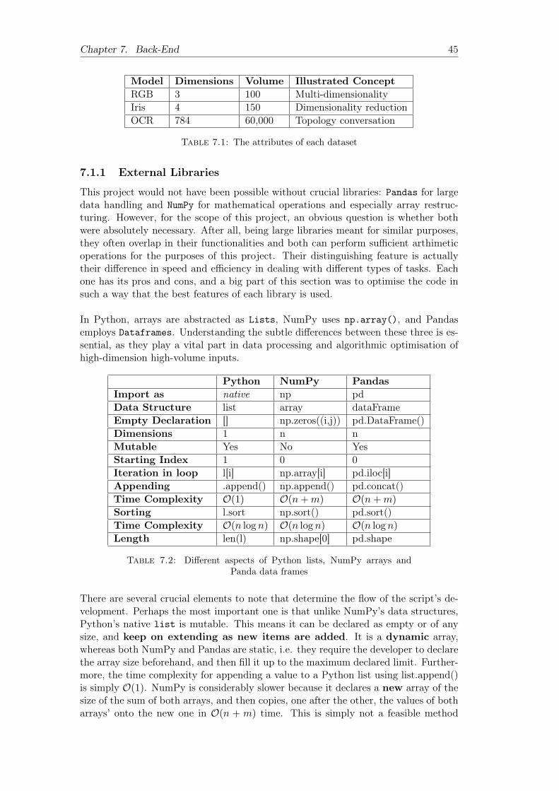
Chapter 7. Back-End 45

Model Dimensions Volume Illustrated ConceptRGB 3 100 Multi-dimensionalityIris 4 150 Dimensionality reductionOCR 784 60,000 Topology conversation

Table 7.1: The attributes of each dataset

7.1.1 External Libraries

This project would not have been possible without crucial libraries: Pandas for largedata handling and NumPy for mathematical operations and especially array restruc-turing. However, for the scope of this project, an obvious question is whether bothwere absolutely necessary. After all, being large libraries meant for similar purposes,they often overlap in their functionalities and both can perform sufficient arthimeticoperations for the purposes of this project. Their distinguishing feature is actuallytheir difference in speed and efficiency in dealing with different types of tasks. Eachone has its pros and cons, and a big part of this section was to optimise the code insuch a way that the best features of each library is used.

In Python, arrays are abstracted as Lists, NumPy uses np.array(), and Pandasemploys Dataframes. Understanding the subtle differences between these three is es-sential, as they play a vital part in data processing and algorithmic optimisation ofhigh-dimension high-volume inputs.

Python NumPy PandasImport as native np pdData Structure list array dataFrameEmpty Declaration [] np.zeros((i,j)) pd.DataFrame()Dimensions 1 n nMutable Yes No YesStarting Index 1 0 0Iteration in loop l[i] np.array[i] pd.iloc[i]Appending .append() np.append() pd.concat()Time Complexity O(1) O(n+m) O(n+m)

Sorting l.sort np.sort() pd.sort()Time Complexity O(n log n) O(n log n) O(n log n)

Length len(l) np.shape[0] pd.shape

Table 7.2: Different aspects of Python lists, NumPy arrays andPanda data frames

There are several crucial elements to note that determine the flow of the script’s de-velopment. Perhaps the most important one is that unlike NumPy’s data structures,Python’s native list is mutable. This means it can be declared as empty or of anysize, and keep on extending as new items are added. It is a dynamic array,whereas both NumPy and Pandas are static, i.e. they require the developer to declarethe array size beforehand, and then fill it up to the maximum declared limit. Further-more, the time complexity for appending a value to a Python list using list.append()is simply O(1). NumPy is considerably slower because it declares a new array of thesize of the sum of both arrays, and then copies, one after the other, the values of botharrays’ onto the new one in O(n + m) time. This is simply not a feasible method

Chapter 7. Back-End 46

when iterating over 60, 000 rows with 784 values each, due to both the time taken andmemory required.

However, a pivotal concept is that Python lists can be very easily and rapidly convertedto NumPy arrays. This is very much the key notion of the back-end development,and also at the heart of working in data science in Python. In fact, you can haveNumPy perform specific operations with a function on a Python list without directlyconverting it. However, this way NumPy would be forced to construct a new arrayand copy its value every single time the function is called, giving a time complexity ofO(k ·(n+m)) where k is the number of times the NumPy function is called. However,it is generally a good practice to directly convert a list to NumPy array only once,after completing the appending-data phase.

Similarly, Pandas’ data structures can also be converted into NumPy arrays, andalso easily be appended to lists.

1 # Import2 import pandas as pd3 import numpy as np4

5 # Declare empty l i s t − O(1)6 myList = [ ]7

8 # Add va lues from Panda dataframe in to empty Python l i s t − O(n)9 f o r i in range ( dataValues . shape ) :

10 myList . append ( dataValues [ i ] )11

12 # Convert l i s t to NumPy array − O(n)13 myArr = np . array (myList )

Listing 7.1: Declaring, filling and converting a Python list to aNumPy array with values from a Panda data frame

If one had to choose the most suitable library for this project, the edge would go toNumPy for its multi-dimensional array manipulation and processing, which are trulyrelevant to this project. Moreover, NumPy works well with Matplotlib, a Python datavisualisation and plotting tool, which is why it was chosen to be the central workingframework. All the data was eventually converted to variables which were compatiblewith NumPy, and the Kohonen algorithm was implemented with it.

The functions that NumPy cannot do efficiently, were delegated to other libraries.Specifically, Pandas was used to read the inputs from a .csv file, as it’s pd.read_csv(‘my_file.csv’) was vastly superior to NumPy’s genfromtxt(‘my_file.csv’,delimiter=‘,’)1, and Python lists were essentially used to fill up arrays with un-known final size. The rest of the implementation takes place primarily using NumPy’sand its following functions.

7.1.2 Principal External Functions

Note that many of these functions can also contain additional parameters not listedhere. Depending on the context and need, the source contains further arguments than

1Fastest Python library to read a CSV file - Stack Exchange. https://softwarerecs.stackexchange.com/questions/7463/fastest-python-library-to-read-a-csv-file. (Accessedon 05/04/2018).

Chapter 7. Back-End 47

those mentioned here for some of these functions.

NumPy:

• np.zeros((i,j)) - Declares a multi-dimensional array of i rows and j columns.

• np.array(myList) - Converts the list myList into an NumPy array.

• np.reshape(m,n) - Reshapes an array from dimensions i,j into m,n.

• np.log(x) - Returns natural logarithm lnx of x.

• np.exp(x) - Returns the value of ex.

• np.sum(myArr) - Returns the sum of the array’s myArr elements.

• np.add(x,y) - Returns the sum of x and y.

• np.max(myArr) - Returns the maximum value of the parameter array myArr.

• np.random.rand(i,j) - Returns random values in shape of i rows and j columns.

• np.savetxt(‘mySavedFile.csv’,myNPArr) - Saves the np array myNpArrayinto the current directory as mySavedFile.csv file.

Pandas:

• read_csv(fileName.csv) - Read data from a fileName.csv file.

Matplotlib:

• plt.scatter(xValues,yValues,s,marker,facecolour,edgecolour) - Plots ascattergraph with values from the NumPy arrays xValues and yValues. Thesize, type and colour of the marker can be customised with the remaining pa-rameters.

• plt.xlabel(‘x-axis-title’) - Inserts a title to the plot’s x axis.

• plt.ylabel(‘y-axis-title’) - Inserts a title to the plot’s y axis.

• plt.title(‘title’) - Inserts a title to the plot.

• plt.show() - Displays the plot after the script is executed.

Argparse:

• argparse.ArgumentParser() - Creates an argument parser.

• argparse.ArgumentParser.add_argument() - Adds an argument to the argu-ment parser.

• argparse.ArgumentParser.parse_args() - Parses all the arguments added tothe argument parser.

Sys:

• sys.exit(1) - Exits the Python script gracefully with error status 1.

Datetime:

• datetime.datetime.now() - Returns current date and time.

Chapter 7. Back-End 48

7.1.3 Variables

• i is the current iteration.

• n_iterations is the iteration limit, i.e. the total number of iterations thenetwork can undergo.

• time_constant is the time constant, used to decay the radius and learning rate.

• x is the row coordinate of the nodes grid.

• y is the column coordinate of the nodes grid.

• w_dist is the (squared) distance between a node and the BMU.

• w is the weight of the connection between the node x,y in the grid, and theinput vector’s instance at iteration i.

• inputsValues is the input vector.

• inputsValues[i] is the input vector’s instance at iteration i.

• l is the learning rate, decreasing with time in the interval [0, 1], to ensure thenetwork converges.

• influence is the influence the neighbourhood function, monotonically decreas-ing and representing a node x,y’s distance from the BMU, has on the learningat step i. It is gradually reduced over time.

• r is the radius of the neighbourhood function, which determines the extent ofthe distance neighbour nodes are examined in the grid. It is gradually reducedover time.

• n is the total number of grid rows

• m is the total number of grid columns

• net[x,y,m] is the nodes grid

• n_classes is the total number distinct classes in input

• labels is the label vector of every input’s instance

7.2 Software Development

7.2.1 Arguments Parser

The implemented algorithm uses several variables, which, if modified, would alteroutcome of the Self-Organising Map, affecting both the value of variables and theirvisualisation. The whole point of this project is to discover and visualise the factorsthat influence and change the outcomes of this algorithm. Additionally, it is a goodideology of software engineering to develop a program which allows modification ofthese parameters with ease.

As such, the developed script allows users to specifically customise arguments, suchas the learning rate and the number of inputs. A neat trick was to develop the scriptsso that these parameters could be modified from the command-line itself, asis the case for many data-focused programs, instead of changing the values directlyin the source code at various places at every adjustment. For this purpose, Python’sargument parser, argparse was selected and came in very handy.

For example, to input the learning rate in the command-line directly, the code would

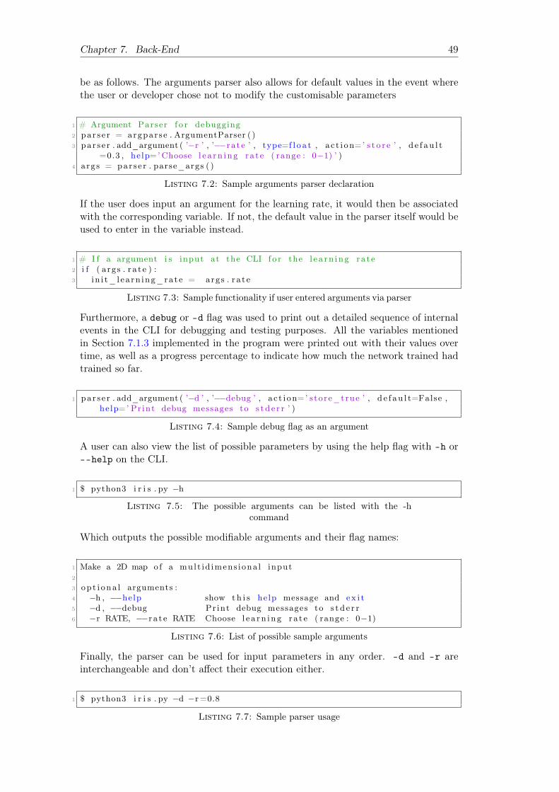
Chapter 7. Back-End 49

be as follows. The arguments parser also allows for default values in the event wherethe user or developer chose not to modify the customisable parameters

1 # Argument Parser f o r debugging2 par s e r = argparse . ArgumentParser ( )3 par s e r . add_argument ( ’−r ’ , ’−−r a t e ’ , type=f l o a t , a c t i on=’ s t o r e ’ , d e f au l t

=0.3 , he lp=’ Choose l e a rn i ng ra t e ( range : 0−1) ’ )4 args = par s e r . parse_args ( )

Listing 7.2: Sample arguments parser declaration

If the user does input an argument for the learning rate, it would then be associatedwith the corresponding variable. If not, the default value in the parser itself would beused to enter in the variable instead.

1 # I f a argument i s input at the CLI f o r the l e a rn i ng ra t e2 i f ( a rgs . r a t e ) :3 i n i t_ l ea rn ing_rate = args . r a t e

Listing 7.3: Sample functionality if user entered arguments via parser

Furthermore, a debug or -d flag was used to print out a detailed sequence of internalevents in the CLI for debugging and testing purposes. All the variables mentionedin Section 7.1.3 implemented in the program were printed out with their values overtime, as well as a progress percentage to indicate how much the network trained hadtrained so far.

1 par s e r . add_argument ( ’−d ’ , ’−−debug ’ , a c t i on=’ store_true ’ , d e f au l t=False ,he lp=’ Pr int debug messages to s t d e r r ’ )

Listing 7.4: Sample debug flag as an argument

A user can also view the list of possible parameters by using the help flag with -h or--help on the CLI.

1 $ python3 i r i s . py −h

Listing 7.5: The possible arguments can be listed with the -hcommand

Which outputs the possible modifiable arguments and their flag names:

1 Make a 2D map o f a mult id imens iona l input2

3 op t i ona l arguments :4 −h , −−help show th i s he lp message and ex i t5 −d , −−debug Pr int debug messages to s t d e r r6 −r RATE, −−r a t e RATE Choose l e a rn i ng ra t e ( range : 0−1)

Listing 7.6: List of possible sample arguments

Finally, the parser can be used for input parameters in any order. -d and -r areinterchangeable and don’t affect their execution either.

1 $ python3 i r i s . py −d −r=0.8

Listing 7.7: Sample parser usage

Chapter 7. Back-End 50

This executes the Python script, and is described in the next sections, which lists theinformation and variables values. The user input parameters such as the learning ratecan indeed be spotted in the output generated via the debug flag.

1 Debug mode ON2 Loading input f i l e s . . .3 Loaded inputs : <c l a s s ’numpy . ndarray ’>4 Loaded l a b e l s : <c l a s s ’numpy . ndarray ’>5 Data normal i sed : Fa l se6 n_classes : 37 n : 1508 m: 49 Network dimensions : ( 2 , )

10 Number o f t r a i n i n g i t e r a t i o n s : 15011 I n i t i a l l e a rn i ng ra t e : 0 . 312 Inputs per c l a s s : 5013 Net <c l a s s ’numpy . ndarray ’>14 I n i t i a l Radius 3 .015 Time constant 136.535883994025616 0%17 1%18 . . .19 99%20 100%21 Rate : 0 . 322 x : (150 , )23 y : (150 , )24 z : (150 , 3)25 BMUs: (150 , 2)26 Saved so r t ed coo rd ina t e s27 Saved so r t ed coo rd ina t e s with no i s e

Listing 7.8: Sample parser usage output

7.2.2 Datasets

For importing and using the original dataset, e.g. the Iris and EMNIST dataset, in-side the Python scripts, they could be downloaded in .csv format from their hostingsites. They could then be referenced by into the script by their path, and thus usedfor training the network.

1 data_path = ’ loca lPath / da t a s e tF i l e . csv ’2 data = pd . read_csv ( data_path )

Listing 7.9: Importing the Iris dataset from a local file using Pandas

This would imply having them in the project directory along with the source code tocompile every time. However, sharing this would be very problematic, as the EMNISTdataset has 188, 000 lines, and weighs around 218Mb. Even as a .zip file this was notan ideal way.

An elegant solution was found in Panda’s documentation which allowed data to beimportant directly for URLs, starting from version 0.19.2, and substantially reducesthe size of the final source code folder.

1 data_path = ’ http :// a rch ive . i c s . uc i . edu/ml/machine−l e a rn ing−databases /i r i s / i r i s . data ’

Chapter 7. Back-End 51

2 data = pd . read_csv ( data_path , encoding=’ utf−8 ’ , header=None )

Listing 7.10: Importing the Iris dataset from URL using Pandas

A subsequent challenge in this method was that the EMNIST dataset was not hostedanywhere online in a .csv format. This was circumvented by uploading the dataon the University of Liverpool server, and hosting them at a public URL http://cgi.csc.liv.ac.uk/~u5es2/EMNIST/. One might think that the data is not se-cure as the website is http not https, but it is important to recall that this datasetis freely available in the public domain, and does not contain any sensitive data. Fur-thermore, the university server files are hosted behind a firewall, which gives it anextra layer of protection.

1 data_path = ’ http :// c g i . c s c . l i v . ac . uk/~u5es2 /EMNIST/Sorted /Train . csv ’2 data = pd . read_csv ( data_path , encoding=’ utf−8 ’ , header=None )

Listing 7.11: Importing the EMNIST dataset from URL usingPandas

The contents of the uploaded .csv files are explained in more detail in Section 7.2.7.

The RGB dataset is generated in the script using random values, and therefore doesnot require an import statement.

1 # Argument Parser f o r debugging2 par s e r = argparse . ArgumentParser ( )3 par s e r . add_argument ( ’− i ’ , ’−−inputs ’ , type=int , a c t i on=’ s t o r e ’ , d e f au l t

=20, he lp=’ Choose number o f t r a i n inputs per c l a s s ( range : 0−2400) ’ )4 args = par s e r . parse_args ( )5

6 # Get value in va r i a b l e7 i f ( a rgs . inputs ) :8 inputsQuant ity = args . inputs9

10 # Generate reques ted quant i ty o f v e c t o r s11 data = np . random . rand int (0 , 255 , ( inputsQuantity , 3) )

Listing 7.12: Sample RGB dataset creation

7.2.3 Normalisation

Once the dataset has been imported, or generated, it should be normalised so thatall inputs features are given the same importance. For example in the Iris dataset,the petals might naturally be longer than the sepals, however the former attributesshouldn’t be given more weight than latter ones while training. Normalising neu-tralises this effect, and additionally, neural networks are much more efficient if theinput values are between 0 and 1.

1 # Constant2 INPUTS_MAX_VALUE = data .max( )3

4 # Normalise and convert from l i s t to array5 inputs = [ ]6 inputs = data/INPUTS_MAX_VALUE7 inputs = np . array ( inputs )

Listing 7.13: Sample RGB data normalisation

Chapter 7. Back-End 52

The input’s max value used for normalisation will be 255 for the RGB and OCRdataset, as they both read colour values, and are even (0-255) across all dimensions ofeach input. This also makes it easier to normalise the whole dataset all at once. Forthe Iris dataset, however, the maximum value used for normalisation will actually bethe maximum value in the dataset for that column, as the variables are on differentscales.

1 # Constant2 INPUTS_MAX_VALUE = data .max( ax i s=0)3

4 # Normalise and convert from l i s t to array5 inputs = [ ]6 inputs = data/INPUTS_MAX_VALUE[ np . newaxis , : ]7 inputs = np . array ( inputs )

Listing 7.14: Sample Iris data normalisation

7.2.4 Kohonen Algorithm Implementation

This section goes through the internal functions developed for the Kohonen algorithmthat are the same for all three models.

1 f o r i in range ( n_i t e ra t i on s ) :2

3 # −−−−−−−−−−−−− INPUT −−−−−−−−−−−−−4 # 1. S e l e c t a input weight vec to r at each step5

6 # This can be random , however s i n c e we ’ re us ing so r t ed inputs , we ’ re7 # proceed ing in a l i n e a r manner through a l l nodes f o r sake o f c l a r i t y8 t = inputsValues [ i , : ] . reshape (np . array ( [m, 1 ] ) )9

10 # −−−−−−−−−−−−− BMU −−−−−−−−−−−−−11 # 2. Find the chosen input vec to r ’ s BMU at each step12 bmu, bmu_idx , d i s t = findBMU( t , net , m)13

14 # −−−−−−−−−−−−− DECAY −−−−−−−−−−−−−15 # 3. Determine t o p o l o g i c a l neighbourhood f o r each step16 r = decayRadius ( in i t_rad ius , i , t ime_constant )17 l = decayLearningRate ( in i t_learn ing_rate , i , i t e r a t i o n s )18

19 # −−−−−−−−−−−−− UPDATE −−−−−−−−−−−−−20 # 4. Repeat f o r a l l nodes in the BMU neighbourhood21 f o r x in range ( net . shape [ 0 ] ) :22 f o r y in range ( net . shape [ 1 ] ) :23

24 # Find weight vec to r25 w = net [ x , y , : ] . reshape (m, 1)26

27 # Get the 2−D di s t anc e ( not Eucl idean as no sq r t )28 w_dist = np . sum( ( np . array ( [ x , y ] ) − bmu_idx) ∗∗ 2)29

30 # I f the d i s t ance i s with in the cur rent neighbourhood rad iu s31 i f w_dist <= r ∗∗2 :32

33 # Calcu la te the degree o f i n f l u e n c e ( based on the 2−D di s t anc e )34 i n f l u e n c e = ge t I n f l u en c e (w_dist , r )35

36 # Update weight :37 new_w = w + ( l ∗ i n f l u e n c e ∗ ( t − w) )

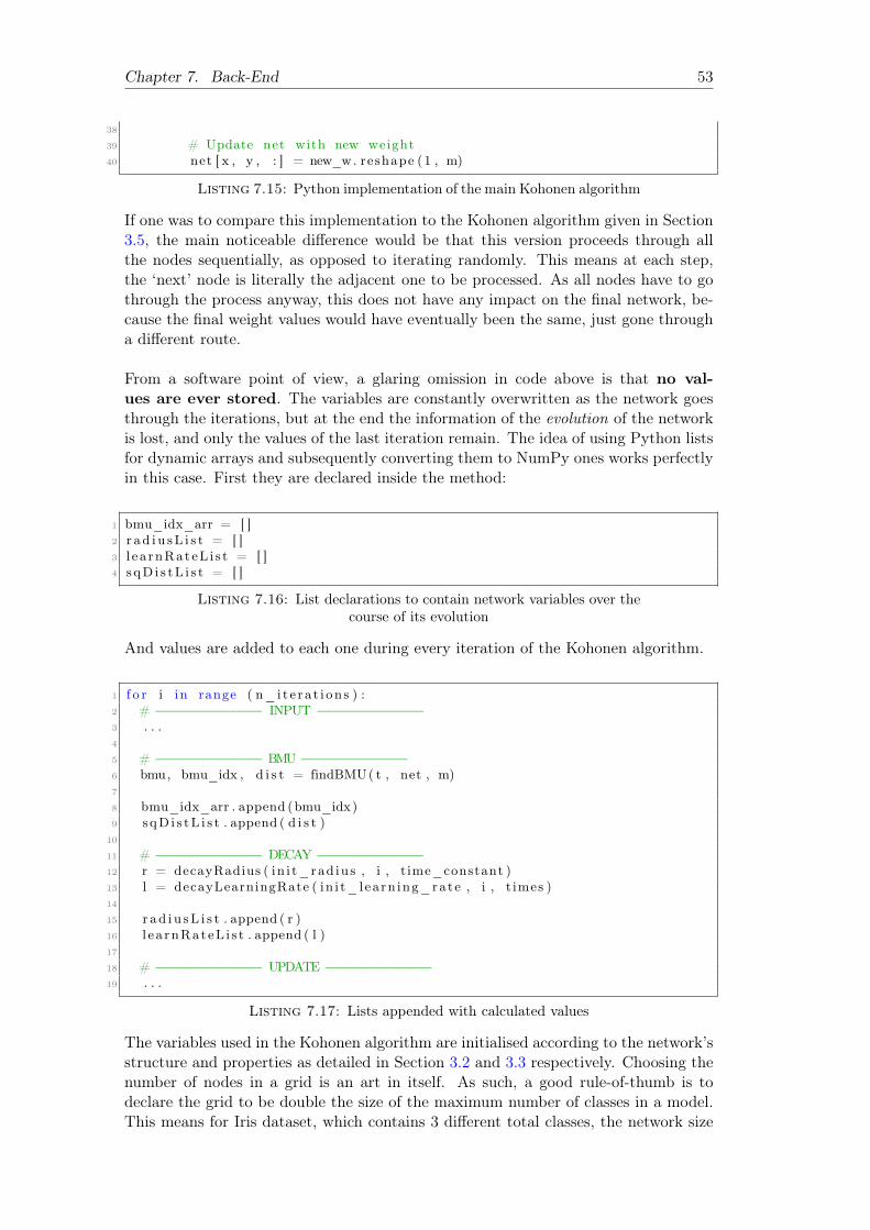
Chapter 7. Back-End 53

38

39 # Update net with new weight40 net [ x , y , : ] = new_w. reshape (1 , m)

Listing 7.15: Python implementation of the main Kohonen algorithm

If one was to compare this implementation to the Kohonen algorithm given in Section3.5, the main noticeable difference would be that this version proceeds through allthe nodes sequentially, as opposed to iterating randomly. This means at each step,the ‘next’ node is literally the adjacent one to be processed. As all nodes have to gothrough the process anyway, this does not have any impact on the final network, be-cause the final weight values would have eventually been the same, just gone througha different route.

From a software point of view, a glaring omission in code above is that no val-ues are ever stored. The variables are constantly overwritten as the network goesthrough the iterations, but at the end the information of the evolution of the networkis lost, and only the values of the last iteration remain. The idea of using Python listsfor dynamic arrays and subsequently converting them to NumPy ones works perfectlyin this case. First they are declared inside the method:

1 bmu_idx_arr = [ ]2 r ad i u sL i s t = [ ]3 l e a rnRateL i s t = [ ]4 s qD i s tL i s t = [ ]

Listing 7.16: List declarations to contain network variables over thecourse of its evolution

And values are added to each one during every iteration of the Kohonen algorithm.

1 f o r i in range ( n_i t e ra t i on s ) :2 # −−−−−−−−−−−−− INPUT −−−−−−−−−−−−−3 . . .4

5 # −−−−−−−−−−−−− BMU −−−−−−−−−−−−−6 bmu, bmu_idx , d i s t = findBMU( t , net , m)7

8 bmu_idx_arr . append (bmu_idx)9 s qD i s tL i s t . append ( d i s t )

10

11 # −−−−−−−−−−−−− DECAY −−−−−−−−−−−−−12 r = decayRadius ( in i t_rad ius , i , t ime_constant )13 l = decayLearningRate ( in i t_learn ing_rate , i , t imes )14

15 r ad i u sL i s t . append ( r )16 l e a rnRateL i s t . append ( l )17

18 # −−−−−−−−−−−−− UPDATE −−−−−−−−−−−−−19 . . .

Listing 7.17: Lists appended with calculated values

The variables used in the Kohonen algorithm are initialised according to the network’sstructure and properties as detailed in Section 3.2 and 3.3 respectively. Choosing thenumber of nodes in a grid is an art in itself. As such, a good rule-of-thumb is todeclare the grid to be double the size of the maximum number of classes in a model.This means for Iris dataset, which contains 3 different total classes, the network size

Chapter 7. Back-End 54

would 6x6. For the model using only digits, the size would 20x20, as there are a totalof 10 digits (0-9).

1 # Weight Matrix2 net = np . random . random ( ( n_classes ∗2 , n_classes ∗2 , m) )3

4 # I n i t i a l Radius f o r the neighbourhood5 i n i t_rad iu s = max( network_dimensions [ 0 ] , network_dimensions [ 1 ] ) / 26

7 # Radius decay parameter8 time_constant = n_i t e ra t i on s / np . l og ( i n i t_rad iu s )

Listing 7.18: Declarations

The functions are based on the formulas given in section 3.6. Recall that the radiusand learning rate have to decrease with time, similar to a exponential function, andthe influence like a Gaussian function.

1 # Decay the neighbourhood rad iu s with time2 de f decayRadius ( i n i t i a l_ r ad i u s , i , t ime_constant ) :3 re turn i n i t i a l_ r a d i u s ∗ np . exp(− i / time_constant )4

5 # Decay the l e a rn i ng ra t e with time6 de f decayLearningRate ( i n i t i a l_ l e a rn i ng_ra t e , i , n_ i t e ra t i on s ) :7 re turn i n i t i a l_ l e a r n i n g_ra t e ∗ np . exp(− i / n_i t e ra t i on s )8

9 # Calcu la te the i n f l u e n c e10 de f g e t I n f l u en c e ( d i s tance , rad iu s ) :11 re turn np . exp(−d i s t anc e / (2∗ ( rad iu s ∗∗2) ) )

Listing 7.19: Functions

And finally, the function to find the BMU, which is called at each iteration in the Ko-honen algorithm, can be implemented as below. Each node is evaluated in the grid isevaluated, until the one which is the most similar to the current input node - mean-ing the one with the smallest Euclidean distance - is chosen and returned as the BMU.

1 de f findBMU( t , net , m) :2 # A 1D array which w i l l conta in the X,Y coo rd ina t e s3 # of the BMU fo r the g iven input vec to r t4 bmu_idx = np . array ( [ 0 , 0 ] )5

6 # Set the i n i t i a l minimum d i f f e r e n c e to l a r g e number7 min_diff = np . i i n f o (np . i n t ) .max8

9 # To compute the high−dimension d i s t ance between10 # the given input vec to r and each neuron ,11 # we c a l c u l a t e the d i f f e r e n c e between the ve c to r s12 f o r x in range ( net . shape [ 0 ] ) :13 f o r y in range ( net . shape [ 1 ] ) :14 w = net [ x , y , : ] . reshape (m, 1)15

16 # Don ’ t sq r t to avoid heavy operat i on17 d i f f = np . sum( (w − t ) ∗∗ 2)18

19 i f ( d i f f < min_diff ) :20 min_diff = d i f f21 bmu_idx = np . array ( [ x , y ] )22

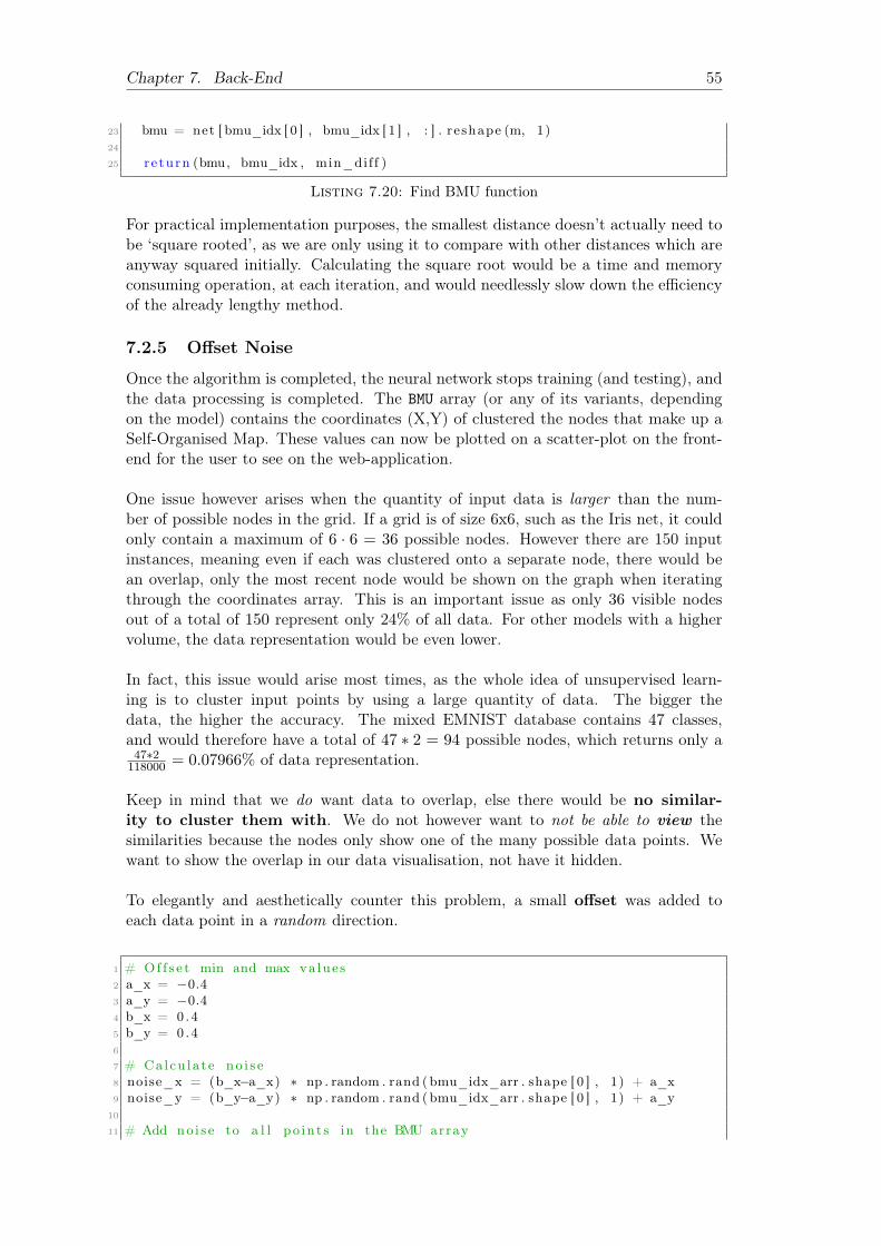
Chapter 7. Back-End 55

23 bmu = net [ bmu_idx [ 0 ] , bmu_idx [ 1 ] , : ] . reshape (m, 1)24

25 re turn (bmu, bmu_idx , min_diff )

Listing 7.20: Find BMU function

For practical implementation purposes, the smallest distance doesn’t actually need tobe ‘square rooted’, as we are only using it to compare with other distances which areanyway squared initially. Calculating the square root would be a time and memoryconsuming operation, at each iteration, and would needlessly slow down the efficiencyof the already lengthy method.

7.2.5 Offset Noise

Once the algorithm is completed, the neural network stops training (and testing), andthe data processing is completed. The BMU array (or any of its variants, dependingon the model) contains the coordinates (X,Y) of clustered the nodes that make up aSelf-Organised Map. These values can now be plotted on a scatter-plot on the front-end for the user to see on the web-application.

One issue however arises when the quantity of input data is larger than the num-ber of possible nodes in the grid. If a grid is of size 6x6, such as the Iris net, it couldonly contain a maximum of 6 · 6 = 36 possible nodes. However there are 150 inputinstances, meaning even if each was clustered onto a separate node, there would bean overlap, only the most recent node would be shown on the graph when iteratingthrough the coordinates array. This is an important issue as only 36 visible nodesout of a total of 150 represent only 24% of all data. For other models with a highervolume, the data representation would be even lower.

In fact, this issue would arise most times, as the whole idea of unsupervised learn-ing is to cluster input points by using a large quantity of data. The bigger thedata, the higher the accuracy. The mixed EMNIST database contains 47 classes,and would therefore have a total of 47 ∗ 2 = 94 possible nodes, which returns only a47∗2

118000 = 0.07966% of data representation.

Keep in mind that we do want data to overlap, else there would be no similar-ity to cluster them with. We do not however want to not be able to view thesimilarities because the nodes only show one of the many possible data points. Wewant to show the overlap in our data visualisation, not have it hidden.

To elegantly and aesthetically counter this problem, a small offset was added toeach data point in a random direction.

1 # Of f s e t min and max va lue s2 a_x = −0.43 a_y = −0.44 b_x = 0 .45 b_y = 0 .46

7 # Calcu la te no i s e8 noise_x = (b_x−a_x) ∗ np . random . rand (bmu_idx_arr . shape [ 0 ] , 1) + a_x9 noise_y = (b_y−a_y) ∗ np . random . rand (bmu_idx_arr . shape [ 0 ] , 1) + a_y

10

11 # Add no i s e to a l l po in t s in the BMU array

Chapter 7. Back-End 56

12 xPlotNoise = np . add (bmu_idx_arr [ : , 0 ] , noise_x [ : , 0 ] )13 yPlotNoise = np . add (bmu_idx_arr [ : , 1 ] , noise_y [ : , 0 ] )

Listing 7.21: Adding offset to each data point

This way, if a single node contained more than one data point, then they would notbe hidden by virtue of being one on top of the other, but in fact ‘scattered’ aroundthe node. The idea is simpler to grasp in a visual form.

(a) A trained SOM without noise (b) A trained SOM with noise

Figure 7.1: By adding an offset to each data point, a considerablyimproved visualisation of the entire dataset is possible.

The difference in quantity of information gathered by glancing at both plots is ofimmense value, and its depth and importance cannot be understated. Visual repre-sentation of data is very striking to the human eye, and a good rendition requires verylittle explanation. Adding noise to each data point was therefore absolutely vital, andperhaps the single most important feature developed in the entire back-end. It singlehandedly increases the quality and value of every single plot generated and viewed bythe user. The quality of the neural network’s training can be assessed to a certaindegree by a simple glimpse at the scatterplot with noise.

7.2.6 Processing Speed vs. the Number of Classes

After implementing and testing the RGB and Iris models of the network, a majorproblem quickly became apparent for the OCR model. The final Self-Organising Mapwould only be produced at the end of all iterations. This was not an issue for datasetswith low dimensions, low data volume, low classes, or even low-dimensions and high-volume, as the data processing would be at worst relatively slow, i.e. a couple ofminutes. However, for datasets with high-volume, high-dimensions and especially alarge number of classes (e.g. 47), the processing time would be very, very long.

The EMNIST dataset, however, contained a total of 47 classes, with a high-volumedata of 112800 instances, each one being of 784 dimensions. The RGB generateddataset, on the other hand, had a low - arbitrary - amount of classes (anything be-tween 3 and 5), 100 instances of each data point of only 3 dimensions each. The Irisdataset had 3 classes, 150 instances of 4 dimensions each.

Although the dimension and volume attribute for each dataset were known and ac-counted for, as shown in the table 7.1, an issue was that the current implementationcreated a nodes grid of 2*n_classes. This means for the EMNIST dataset, therewas a grid of (2 · 47) ∗ (2 · 47) = 942 = 8, 836 nodes in total, and each single one’sEuclidean distance over 784 dimensions was calculated. In simpler words, calculating

Chapter 7. Back-End 57

the difference between 2 arrays, of 784 values each, a total of 8, 836 times is what madethe training laboriously slow. Even without calculating the square of each difference,the process was slow enough to easily last several hours for around 10,000 inputsonly.

1 f o r x in range ( net . shape [ 0 ] ) :2 # Net shape i s the l ength ( and width ) o f nodes g r id . In EMNIST ’ s case

the s i z e o f the g r id i s 94x94 , which g i v e s a t o t a l o f 8836 i t e r a t i o n s.

3 f o r y in range ( net . shape [ 1 ] :4 w = net [ x , y , : ] . reshape (m, 1)5 d i f f = np . sum( (w − t ) ∗∗ 2)

Listing 7.22: The section of findBMU() function which took agigantic amount of time

As learnt by this practical experience, the size of the network is the most im-portant factor in determining the feasibility of a network’s training. If itwas decided that the size should follow a certain unalterable rule of thumb - that thelength and width of a network should be double the size of its total number of classes- then the only way possible to make this network’s convergence feasible was to reduceits total input data. 150 input data instances were sufficient to converge and visualisethe Iris dataset, and the RGB model could easily go up to 60,000 instances and pro-duce a stabilised network (by virtue of each instance being very low-dimension andthe network having an overall small sized grid). Surely a quantity between severalhundred and a few thousand should be able to converge a network, even with 94x94grid.

Thus, the ideal solution was to change the implementation in a way such that onlythe first 20 values of each class was taken in as input data, totalling approximately areasonable thousand values (47 ·20 = 940). And after labourious debugging and inputdata visualisation, therein was discovered the biggest challenge and set-back ofthe entire project: the EMNIST’s dataset, totalling 112,800 data instances of 784dimensions each, were not sorted according to their class. They entire databasewas ordered randomly, making it impossible to reduce the total number of inputs foreach class when training the network.

The magnitude of this realisation simply cannot be understated. This meant therewas no way to work with the principal dataset of the project without waiting hourson end for the network to finish training for a single test, and even then there couldbe minor programming errors which could ‘ruin the batch’, so to speak. This tookan enormous toll on the productivity and advancement of the realisation of the im-plementation, and was the single biggest cause of delay against the planned timeline.A string of alternative fixes, ingenious ‘hacks’, and innovative work-arounds were at-tempted under intense pressure in order to find a feasible solution for this issue withina manageable time-frame.

An obvious resolution was not to reduce the quantity of input data of each class, butto instead take a slightly bigger chunk of the total dataset, so that there was enough ofa margin to encompass every class’s input values at least a handful of times, and stillhave a total number of input instances not going beyond a couple of thousand. Thiswould nonetheless take several minutes to an hour to compute, but could be optimisedto find the perfect ratio between inputs of each class and the total computational time.

Chapter 7. Back-End 58

However, this method proved to be unsuccessful, as a network simply cannot convergewith a couple of thousand total inputs, as they represent only around 20 instancesof each class, which is very low to distinguish between data of 784 dimensions. Fur-thermore, the slice of data being taken from the original large dataset was too smallto offset the randomness of each class. Some classes were repeated too often, andsome almost none. This would lead to a distorted and converged network. Finally,a possibility was simply that the network was not convergable for a large number oftotal classes. After all, Kohonen networks were used to visualise and find pattern indata that overlapped in a few instances. In the case of EMNIST, the full dataset wastoo large with 47 different classes, along with being too long to train and converge.However, it seems counter-intuitive to think that there were perhaps not enough sim-ilarities between a large number of classes, as logically they should have more overlapthan datasets with fewer classes.

An alternative way to ‘hack’ this problem, was to use several machines to processdifferent networks, each run with different parameters values, and use each result tosee and understand which hypothesis held truth to determine the principal factor thatcaused this non-convergence.

Again, this proved to be an impossible tasks for several logistical reasons. First of all,the number of available machines was very low. Secondly, all of them needed to havethe version of Python and its various libraries such as NumPy and Pandas installed.If a machine was non-unix based, then another set-back would take place due to theadditional work load of configuring a Windows machine. Finally, any update to theoverall script development would have to be made on the other machine as well. Themanagement and synchronisation of the scripts would be an absurdly strenuous taskto conduct. It was simply not a feasible solution, both technically and logistically tobreak down an issue over several machines in order to try and understand the cause ofa neural network’s convergence and potentially use the results to overcome the issue.It was mentally taxing enough to work on such a problem on a single machine, withconstant minor updates to the developing scripts.

The only way to overcome this problem was then to sort the data. If all 112,800input could be sorted into 47 different arrays, with each one containing only the in-stances belonging to that distinct class, then we could a chose a specific amount ofinputs all sorted arrays. Moreover, we could see if the non-convergence of a networkwas really due to a high grid size, and if so find the limit, by first only training asubset of the EMNIST dataset which only contained digits, and therefore only 10total classes. Then the same could be tested on only the alphabets in the EMNISTdataset, which would have 26 classes, before finally attempting the colossal 47 classes.Sorting the data, as often restated in Computer Science education, was the key notonly to implementing the OCR model of Kohonen’s neural network but also the findinsights of the properties and nature of this algorithm.

7.2.7 Data Sorting

The first step to sorting the data was knowing that there were indeed an equal amountof inputs for each class, specifically 112800/40 = 2400 instances. Then, there weretwo ways of proceeding: manually declaring 47 arrays, and using an insertion sort

Chapter 7. Back-End 59

algorithm to iterate over all 47 classes, and appending to the relevant array the in-stance that belonged to that class. This can be determined using the array labels,which thankfully contains the label of each input instance’s class. It did not feel like‘smart’ programming at all to declare such a large amount of arrays. Furthermore,insertion sort is a basic sorting algorithm and would take at best Θ(n) and at worstO(n2) iterations to complete.

A series of alternative ways were again tested, such as using Python dictionaries,47 of which can be easily declared by a single for-loop. However, in each alternativemethod, the core issue that would arise was that it was simply not possible to declarevariable names with other variables. One just cannot use a for-loop to name arrayswith strings.

Instead, the manual way of declaring arrays and using the unsorted data’s labelsto sort them into their respective classes’s array was implemented with success.

1 # Read unsorted raw data2 data_path = ’ path/To/UnSorted/Data . csv ’3 data = pd . read_csv ( data_path )4

5 # Create l i s t s per c l a s s6 arr_0 = [ ]7 arr_1 = [ ]8 . . .9 arr_46 = [ ]

10

11 # Sort and append accord ing to c l a s s12 f o r i in range ( data . shape [ 0 ] ) :13 i f data . i l o c [ i ,0]==0:14 arr_0 . append ( data . i l o c [ i , 1 : ] )15 e l i f data . i l o c [ i ,0 ]==1:16 arr_1 . append ( data . i l o c [ i , 1 : ] )17 . . .18 e l i f data . i l o c [ i ,0]==47:19 arr_47 . append ( data . i l o c [ i , 1 : ] )20

21 # Merge in order in to main l i s t22 so r t ed Input s . extend ( arr_0+arr_1+.. .+ arr_47 )23

24

25 # Make so r t ed l a b e l s l i s t26 i = 027 f o r x in range (0 , data . shape [ 0 ] , max_inputs_per_class ) :28 f o r y in range (max_inputs_per_class ) :29 so r t edLabe l s . append ( i )30 i=i+131

32 # Convert both l i s t s to NumPy arrays33 so r t ed Input s = np . array ( so r t ed Input s )34 so r t edLabe l s = np . array ( so r t edLabe l s )35

36 # Export so r t ed c l a s s e s37 np . savetxt ( save_path+’ SortedInputs . csv ’ , sor tedInputs , fmt=’%d ’ ,

d e l im i t e r=’ , ’ )38 np . savetxt ( save_path+’ SortedLabe l s . txt ’ , so r tedLabe l s , fmt=’%d ’ )

Listing 7.23: Compact view of the sorting script implementation

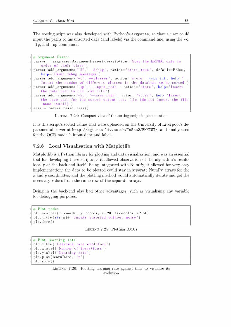
Chapter 7. Back-End 60

The sorting scipt was also developed with Python’s argparse, so that a user couldinput the paths to his unsorted data (and labels) via the command line, using the -c,-ip, and -sp commands.

1 # Argument Parser2 par s e r = argparse . ArgumentParser ( d e s c r i p t i o n=’ Sort the EMNIST data in

order o f t h e i r c l a s s ’ )3 par s e r . add_argument ( ’−d ’ , ’−−debug ’ , a c t i on=’ store_true ’ , d e f au l t=False ,

he lp=’ Pr int debug messages ’ )4 par s e r . add_argument ( ’−c ’ , ’−−c l a s s e s ’ , a c t i on=’ s t o r e ’ , type=int , he lp=’

I n s e r t the number o f d i f f e r e n t c l a s s e s in the database to be so r t ed ’ )5 par s e r . add_argument ( ’−ip ’ , ’−−input_path ’ , a c t i on=’ s t o r e ’ , he lp=’ I n s e r t

the data path to the . csv f i l e ’ )6 par s e r . add_argument ( ’−sp ’ , ’−−save_path ’ , a c t i on=’ s t o r e ’ , he lp=’ I n s e r t

the save path f o r the so r t ed output . csv f i l e ( do not i n s e r t the f i l ename i t s e l f ) ’ )

7 args = par s e r . parse_args ( )

Listing 7.24: Compact view of the sorting script implementation

It is this script’s sorted values that were uploaded on the University of Liverpool’s de-partmental server at http://cgi.csc.liv.ac.uk/~u5es2/EMNIST/, and finally usedfor the OCR model’s input data and labels.

7.2.8 Local Visualisation with Matplotlib

Matplotlib is a Python library for plotting and data visualisation, and was an essentialtool for developing these scripts as it allowed observation of the algorithm’s resultslocally at the back-end itself. Being integrated with NumPy, it allowed for very easyimplementation: the data to be plotted could stay in separate NumPy arrays for thex and y coordinates, and the plotting method would automatically iterate and get thenecessary values from the same row of the separate arrays.

Being in the back-end also had other advantages, such as visualising any variablefor debugging purposes.

1 # Plot nodes2 p l t . s c a t t e r ( x_coords , y_coords , s=20, f a c e c o l o r=zPlot )3 p l t . t i t l e ( s t r (n)+’ Inputs unsorted without no i s e ’ )4 p l t . show ( )

Listing 7.25: Plotting BMUs

1 # Plot l e a rn i ng ra t e2 p l t . t i t l e ( ’ Learning ra t e evo lu t i on ’ )3 p l t . x l ab e l ( ’Number o f i t e r a t i o n s ’ )4 p l t . y l ab e l ( ’ Learning ra t e ’ )5 p l t . p l o t ( learnRate , ’ r ’ )6 p l t . show ( )

Listing 7.26: Plotting learning rate against time to visualise itsevolution

61

Chapter 8

Linking Front to Back End

Finally, this chapter summarises how the front and back end were linked, specificallythe data structures and how the data flowed from one point to another depending onuser inputs and back-end outputs.

8.1 Incompatibility

Till now, all the diverse challenges encountered of various difficulties were eventuallysolved, or accounted for, one way or the other. Some were were purely cosmetic, suchas styling each HTML web-page using CSS and JavaScript, requiring only diligent test-ing and updating. Others were more technically challenging but nonetheless engaging,necessitating theoretical Computer Science skills, such as algorithm complexity anal-ysis, as well as a certain degree of creativity to solve in an elegant manner. Some weresubstantially more challenging to simply identify, and then gruelling to solve, such asdata sorting, requiring a certain abstraction, back-tracking, re-developing parts of thesoftware, and general meticulousness. None of these problems were fundamentallyunsolvable, as the main deciding factor was simply the time, energy, and strategyrequired to overcome them.

There was, however, one underlying technical problem which could not be solved.The issue stems from the general incompatibility between Python and JavaScript.These two programming languages were fundamental to this project, without whichthis project would not have been the same. However, they do not communicate wellat all, as they were not originally ever meant to interact. JavaScript was nativelybuilt to be part of the three core technologies of the World Wide Web, along withHTML and CSS, and is also proficient at working with a PHP back-end. Python, ahigh-level general purpose programming language is good at a lot of things, includingweb-development with frameworks such as Django and Flask, but is not directlycompatible with JavaScript. Flask can host JavaScript files, but to send data froma Python script to a JavaScript one is nonetheless complex. There have been manyattempts to create a simpler way of linking the two, but most of them have eventuallyresulted in awkward and unsuitable implementations for important projects.

When designing this project, neither language could be omitted, as JavaScript isindispensable for web-scripting, and the alternatives to Python for designing a math-ematical back-end would have been very limited without data specific libraries such asNumPy and Pandas. Undertaking a data science project without employing Pythonwould have sorely restricted the scope, modernity and originality of the project.

Consequently, the ambitiousness of this project resulted some incompatibility, oneof which was particularly troublesome as it related to one of the core features this

Chapter 8. Linking Front to Back End 62

project promised: direct interactivity between the user and Kohonen model. Indeed,although components were build with JavaScript to take in a user’s hand-drawn inputson the front-end, they could not be sent to the back-end model in a straightforwardand elegant way. Similarly, the back-end could not directly transfer back the neuralnetwork’s outputs to JavaScript, although this particular direction of flow was slightlymitigated by finding a round-about way, further explained in the next chapter.

This is why, the user input data on the canvas does not return any data, despitesignificant time and work going into converting the drawn strokes to data values ofthe correct shape and size.

Despite being a very interactive feature, the input would have only been a singleinput instance, where as the EMNIST dataset provided over hundred thousands suchvalues. It is important to remember that the implemented network is fully capableof handling input data, at any scale, but simply could not receive the data from theuser. This problem was on a structural and systems level, due to the complex incom-patibility between the polished front-end and highly developed back-end, and not dueto one single error. If one were to manually transfer the user’s letter data to a .csvfile into the Python script, the network could successfully cluster that input.

8.2 Data structures

This section quickly highlights how the front-end was able to read the Python outputvalues, despite the linking not working in the other direction.

By writing the calculated Python values to a local .csv file in the correct relativerepository, these could be read by the JavaScript every time a new page was loaded.

Figure 8.1: Flow of data between front and back ends

8.3 Data Visualisation

The first and most important goal was to use the output data calculated by the Ko-honen back-end model, by transferring it to the front end, and representing it in avisual, comprehensive and easy-to-grasp way.

D3.js was chosen as front-end plotting library as it was very effective at data vi-sualisation. Similar to Bootstrap, D3.js is a continuously updating library, with new

Chapter 8. Linking Front to Back End 63

versions being released every few months. D3’s v4 release was used when researchingthe library and understanding it’s API, however v5 was the final version used for theimplementation.

At this point, all the sorting, processing, and number crunching was completed. Allthat was left was to plot the (X,Y) coordinates list of the BMUs onto a 2D graph,as previously done locally on Python’s Matplotlib. However, this proved to be anunexpectedly and considerably challenging task, and became a critical cause for delayin adding more textual explanations and informations on the website.

The difficulty was mostly due to the nature of the JavaScript library itself. De-spite its popularity, D3.js is not recommended for beginners on account of its verysteep learning curve. Furthermore, it’s Github-based API documentation was hard tounderstand, navigate, and lacking examples for such a dense reference. The constantupdates also didn’t help, as many of the examples given for D3 on other websitesreferred to older versions and were thus useless at the time.

An easy option was to simply avoid D3 altogether and circumvent the problem en-tirely by using a different plotting library. Google Charts, Plotly.js, Chartist.js andespecially Chart.js were all considered as alternatives, but all permutations led to onetechnical issue or the other. Notably, one sticking point for most other libraries wasthat the points were to be read from a local file in .csv format, as opposed to a JSONformat. Additionally, those which did offered little customisation tools in particularfor scatter-plots, which, on top of being plotted, needed to be coloured according toits class value and ideally even display mouse-over text. Therefore, despite the toughlearning curve, an exceptional effort was made to understand the technicalities andpower through the material in a tight period of time in order to be completed by thedemonstration deadline. Ultimately, this challenging endeavour was successful, andthe details hereunder give an insight to the technicalities of D3.js that were overcome.

First of all, unlike most JavaScripts declared at the end of the <body> tag, D3 hadto be important in the header along with the Bootstrap and personal CSS reference,because it is directly called as soon as the page is loaded.

1 <head>2 <!−− D3 . j s −−>3 <s c r i p t s r c=" https : // d3 j s . org /d3 . v5 . min . j s "></ s c r i p t>4 </head>

Listing 8.1: Importing D3.js in the HTML header

Then the code has constructed with the following declared elements: margins, axis,SVGs, and finally plotting the graphs by reading the .csv data files.

1 // Margins2 var margin = {top : 20 , r i g h t : 10 , bottom : 20 , l e f t : 15} ,3 width = 600 − margin . l e f t − margin . r i ght ,4 he ight = 300 − margin . top − margin . bottom ;5

6 // Axis7 var x = d3 . s c a l eL i n e a r ( )8 . range ( [ 0 , width ] ) ;9

10 var y = d3 . s c a l eL i n e a r ( )

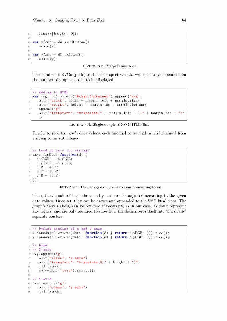
Chapter 8. Linking Front to Back End 64

11 . range ( [ he ight , 0 ] ) ;12

13 var xAxis = d3 . axisBottom ( )14 . s c a l e ( x ) ;15

16 var yAxis = d3 . a x i sL e f t ( )17 . s c a l e ( y ) ;

Listing 8.2: Margins and Axis

The number of SVGs (plots) and their respective data was naturally dependent onthe number of graphs chosen to be displayed.

1 // Adding to HTML2 var svg = d3 . s e l e c t ("#chartContainer" ) . append ("svg" )3 . a t t r ("width" , width + margin . l e f t + margin . r i g h t )4 . a t t r ("height" , he ight + margin . top + margin . bottom )5 . append ("g" )6 . a t t r ("transform" , "translate(" + margin . l e f t + "," + margin . top + ")"

) ;

Listing 8.3: Single sample of SVG-HTML link

Firstly, to read the .csv’s data values, each line had to be read in, and changed froma string to an int integer.

1 // Read as ints not strings2 data . forEach ( function (d) {3 d .xRGB = +d .xRGB;4 d .yRGB = +d .yRGB;5 d .R = +d .R6 d .G = +d .G;7 d .B = +d .B;8 }) ;

Listing 8.4: Converting each .csv’s column from string to int

Then, the domain of both the x and y axis can be adjusted according to the givendata values. Once set, they can be drawn and appended to the SVG html class. Thegraph’s ticks (labels) can be removed if necessary, as in our case, as don’t representany values, and are only required to show how the data groups itself into ‘physically’separate clusters.

1 // Define domains of x and y axis2 x . domain ( d3 . extent ( data , function (d) { return d .xRGB; }) ) . n i c e ( ) ;3 y . domain ( d3 . extent ( data , function (d) { return d .yRGB; }) ) . n i c e ( ) ;4

5 // Draw6 // X-axis7 svg . append ("g" )8 . a t t r ("class" , "x axis" )9 . a t t r ("transform" , "translate(0," + he ight + ")" )

10 . c a l l ( xAxis )11 . s e l e c tA l l ("text" ) . remove ( ) ;12

13 // Y-axis14 svg1 . append ("g" )15 . a t t r ("class" , "y axis" )16 . c a l l ( yAxis )

Chapter 8. Linking Front to Back End 65

17 . s e l e c tA l l ("text" ) . remove ( ) ;

Listing 8.5: X and Y axis

Finally, we can plot each data point using the (X,Y) coordinates in the data as a circlewith a chosen radius. Additionally, we can colour each one according to its class.

1 svg . s e l e c tA l l (".dot" )2 . data ( data )3 . en te r ( ) . append ("circle" )4 . a t t r ("class" , "dot" )5 . a t t r ("r" , 3 . 5 )6 . a t t r ("cx" , function (d) { return x (d .xRGB) ; })7 . a t t r ("cy" , function (d) { return y (d .yRGB) ; })8 . s t y l e ("fill" , function (d) {return d3 . rgb (d .R, d .G, d .B) ; })9 }) ;

Listing 8.6: Plotting the scatterplot circles for RGB dataset

Additionally, the a tooltip can be used for mouseovers.

1 var t o o l t i p = d3 . s e l e c t ("#chartContainer" ) . append ("div" )2 . a t t r ("class" , "tooltip" )3 . s t y l e ("opacity" , 0) ;

Listing 8.7: Mouse hover tooltip appended to html div

The clever part here was the use of the HTML tag <spanstyle=’color:"#";’> con-taining the individually read R,G,B values. An unrelated complication was the offsetvalue by exaggerated by the Bootstrap columns grid structure. Similar to the offsetissue for the canvas, intense debugging was necessary simply to find the cause of theproblem. Once understood, a partial solution was successfully implemented. The ex-tra offset caused by the offset Bootstrap column had to be deducted from the page’seventY value using jQuery: d3.event.pageY-$(this).parent().offset().top.

1 // Mouseover Event Handler2 var t ipMouseover = function (d) {3

4 var html = "<span style=’color:" + d3 . rgb (d .R, d .G, d .B) + ";’>" + d .l a b e l ;

5

6 t o o l t i p 1 . html ( html )7 . s t y l e ("left" , ( d3 . event . pageX) + "px" )8 . s t y l e ("top" , ( d3 . event . pageY − $ ( this ) . parent ( ) . o f f s e t ( ) . top ) + "px

" )9 . t r a n s i t i o n ( )

10 . durat ion (200) // ms11 . s t y l e ("opacity" , . 9 )12 } ;

Listing 8.8: Mouse hover tooltip’s text content coloured accordingto class

The mouseover function is ended when the cursor leaves the data circle, and gentlyfaded out.

1 // Mouseout event handler2 var tipMouseout = function (d) {

Chapter 8. Linking Front to Back End 66

3 t o o l t i p . t r a n s i t i o n ( )4 . durat ion (300) // ms5 . s t y l e ("opacity" , 0) ;6 } ;

Listing 8.9: Mouse out

Each of the 3 dataset’s plots were written in individual JavaScript files using the D3library. They’re named plot.js, plotIris.js, and plotRGB.js.

Figure 8.2: A page with four different D3 charts

8.4 Server deployment

As it turned out, Flask cannot be deployed on a server, at least not without beingthoroughly knowledgeable on third-party Web Server Gateway Interfaces, such asHeroku or OpenShift, which were beyond the scope and intend of this project. Flaskis in fact mostly used for local development and testing purposes only, and thereforethis project was chosen to be developed for local-hosting purposes only as well. Thiswas indeed an unfortunate development with regards to sharing the web-applicationwith other users, as was originally intended.

67

Chapter 9

Testing

9.1 Test Results

The following is the testing results of the different scripts. Each test ID was executedwith the command $Python3ScriptName.py following by any extra CLI parameter,such as -d. The parameters for each test case is given in the table, and a blank valuerepresents no additional argument being parsed.

9.1.1 RGB

ID Data Data Type Expected Result Success?1 (Blank) Correct Successful build YES2 -i Erroneous Native error message YES3 -i= Erroneous Native error message YES4 -i=0 Erroneous Implemented error message YES5 -i=-1 Erroneous Implemented error message YES6 -i=0.5 Erroneous Native error message YES7 -i=-0.5 Erroneous Native error message YES8 -i=100 Correct Successful build YES9 -r Erroneous Native error message YES10 -r= Erroneous Native error message YES11 -r=0 Erroneous Implemented error message YES12 -r=-1 Erroneous Implemented error message YES13 -r=0.5 Correct Successful build YES14 -r=1 Correct Successful build YES15 -r=1.5 Erroneous Implemented error message YES16 -d Correct Successful build YES17 -d-i=100 Correct Successful build YES18 -d-r=0.3 Correct Successful build YES19 -r=0.3-i=100 Correct Successful build YES20 -d-r=0.3-i=100 Correct Successful build YES

Table 9.1: RGB script tests

Chapter 9. Testing 68

9.1.2 Iris

ID Data Type Expected Result Success?1 (Blank) Correct Successful build YES2 -r Erroneous Native error message YES3 -r= Erroneous Native error message YES4 -r=0 Erroneous Implemented error message YES5 -r=-1 Erroneous Implemented error message YES6 -r=0.5 Correct Successful build YES7 -r=1 Correct Successful build YES8 -r=1.5 Erroneous Implemented error message YES9 -d Correct Successful build YES10 -d-r=0.3 Correct Successful build YES

Table 9.2: Iris script tests

9.1.3 OCR

ID Data Type Expected Result Success?1 (Blank) Correct Successful build YES2 -d Correct Successful build YES3 -r Erroneous Native error message YES4 -r= Erroneous Native error message YES5 -r=0 Erroneous Implemented error message YES6 -r=-1 Erroneous Implemented error message YES7 -r=0.5 Correct Successful build YES8 -r=1 Correct Successful build YES9 -r=1.5 Erroneous Implemented error message YES10 -iTr=100 Correct Successful build YES11 -iTr=0 Correct Successful build YES12 -iTr=-1 Erroneous Implemented error message YES13 -iTr=2400 Correct Successful build YES14 -iTr=2401 Erroneous Implemented error message YES15 -iTe=100 Correct Successful build YES16 -iTe=0 Correct Successful build YES17 -iTe=-1 Erroneous Implemented error message YES18 -iTe=2400 Correct Successful build YES19 -iTe=2401 Erroneous Implemented error message YES20 -t=d Correct Successful build YES21 -t=l Correct Successful build YES22 -t=c Correct Successful build YES23 -t=z Erroneous Implemented error message YES24 -d-iTr=100 Correct Successful build YES25 -d-iTe=100 Correct Successful build YES26 -d-r=0.3 Correct Successful build YES27 -d-r=0.3-iTr=100 Correct Successful build YES28 -d-r=0.3-iTr=100-iTe=100 Correct Successful build YES29 -d-r=0.3-iTr=100-iTe=100-t=d Correct Successful build YES

Table 9.3: OCR script tests

Chapter 9. Testing 69

As shown above, the scripts show error handling, and graceful exit for all the caseswhen a user enters an incorrect or invalid parameter.

The full outputs of each cases can be seen in Appendix G, along with the detailsof all hardware and software used for testing.

70

Chapter 10

Results

This chapter presents an overview of plots generated by the Python scripts. They canbe seen in full detail in Appendix H.

10.1 RGB

The following parameters were used to generate the sample plots shown below:

$python3RGB.py-d-i=1000

(a) Data before clustering (b) Data after clustering

(c) Data before clustering with noise (d) Data after clustering with noise

Figure 10.1: RGB model plotted with 1000 inputs

10.2 Iris

The following parameters were used to generate the sample plots shown below:

$python3iris.py-d-r=0.3

Chapter 10. Results 71

(a) Radius evolution over time (b) Learning rate evolution over time

Figure 10.2: Model’s radius and learning rate evolution over time

(a) Data before clustering (b) Data after clustering

(c) Data before clustering with noise (d) Data after clustering with noise

Figure 10.3: Iris dataset plotted with 0.3 learning rate

(a) Radius evolution overtime

(b) Learning rate evolutionover time (c) BMU distance over time

Figure 10.4: Model’s radius, learning rate and squared distance evo-lution over time

Chapter 10. Results 72

10.3 OCR

10.3.1 Digits

The following parameters were used to generate the sample plots shown below:

$python3som.py-r=0.3-iTr=100-iTe=10t=d

Figure 10.5: The legend of each letter used for the graphs below

Chapter 10. Results 73

(a) Train data before clustering (b) Train data after clustering

(c) Train data before clustering with noise (d) Train data after clustering with noise

Figure 10.6: Digits dataset plotted with 100 training and 10 testinginputs with 0.3 learning rate (Part 1)

(a) Test data before clustering (b) Test data after clustering

(c) Test data before clustering with noise (d) Test data after clustering with noise

Figure 10.7: Digits dataset plotted with 100 training and 10 testinginputs with 0.3 learning rate (Part 2)

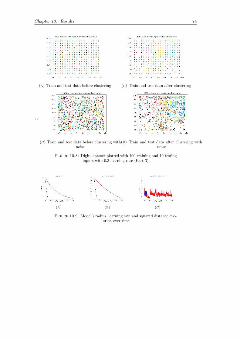
Chapter 10. Results 74

(a) Train and test data before clustering (b) Train and test data after clustering

//

(c) Train and test data before clustering withnoise

(d) Train and test data after clustering withnoise

Figure 10.8: Digits dataset plotted with 100 training and 10 testinginputs with 0.3 learning rate (Part 3)

(a) (b) (c)

Figure 10.9: Model’s radius, learning rate and squared distance evo-lution over time

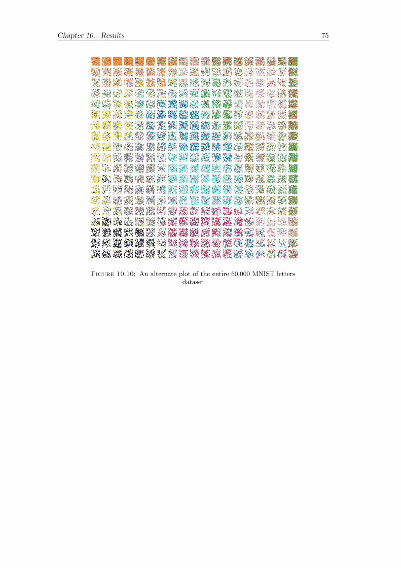
Chapter 10. Results 75

Figure 10.10: An alternate plot of the entire 60,000 MNIST lettersdataset

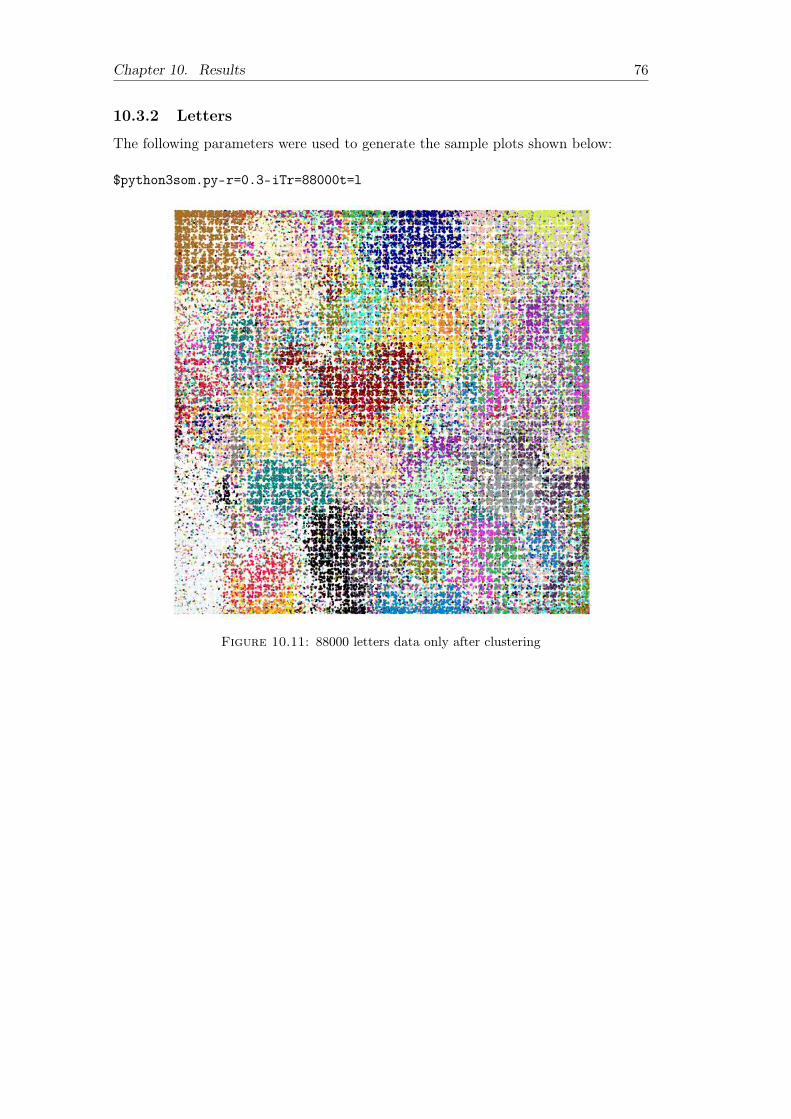
Chapter 10. Results 76

10.3.2 Letters

The following parameters were used to generate the sample plots shown below:

$python3som.py-r=0.3-iTr=88000t=l

Figure 10.11: 88000 letters data only after clustering

77

Chapter 11

Evaluation

To critically assess a project as a whole, one must compare it to the tasks it set outto accomplish at the very beginning. This chapter attempts to give insights on theproject’s overall success by measuring its results against its original goals, coupleswith personal opinion and 3rd party feedback.

11.1 Evaluation Design

11.1.1 Evaluation Criteria

Firstly, it should be ensured that the overall features are working correctly individu-ally and collectively in a asynchronous system.

Secondly, basic user interface and experience guidelines should always work, i.e. click-ing on a button should lead to the correct page corresponding to it, most unexpectedexceptions should be caught, and the website should be able to display ‘error pages’in case of unforeseen crashes rather than native browser alerts.

Additionally, the loading times such as when launching the website, submitting theinput, and visualising the training dataset should all be to a reasonable standard for2018 and in the same league as other similar applications.

Finally, the website should not be invasive in any manner, and only the essentialpermissions should ever be requested. The privacy of the user should be respectedno matter what, and absolutely no tracking or data collecting should be done on thevisitors.

11.1.2 Assessment Criteria

Assessing many of the criteria on efficiency could simply be a straightforward caseof measuring response-time(s) of pages, images, and graphics on various devices andbrowsers with different memories.

For the requested permissions, security certificates and RAM usage, the the browser’sdeveloper console and the device’s task manager could be checked for detailed infor-mation, as another way of assessing the system.

11.2 Critical Evaluation

Each planned feature, given in italics, is evaluated against the final implementation.

Chapter 11. Evaluation 78

11.2.1 Essential Features

• The website should have an interactive ‘Draw’ page where users can draw theirletter on a Graphical User Interface(GUI) canvas and have the website processand display which letter it is, by interacting with the ANN model.

• This was implemented on both ends. The front-end could take user input dataand convert it to a re-sized 28x28 pixel data value in an 784-dimensional ar-ray. The back-end could take in input instances of the same size and output aBest Matching Unit node’s (X,Y) coordinates. However, although they workedindividually, the data could not be sucessfully passed through to one another.Unfortunate, as each component’s implementation was fully developed, an infacteven customised to be able to take in several characters as inputs on a singlecanvas.

• The website should display the neural network’s topological map of input data tothe user based on training (and/or testing) data.

• Fully developed and implemented with Python and D3.js scripts. Took sub-stantial time for both, but topological map can be viewed both on the front-endHTML or on Python’s local Matplotlib.

• The website should highlight where your input would be placed on the displayedtopological map.

• This was also implemented for the user’s canvas data, but cannot be shownas it wasn’t functional. The testing and training data however is correctlydistinguished by crosses and dots.

• The website should have a ‘Learn’ page which displays animations or clickablediagrams of neural networks and SOMs, to show how weights are adjusted andconverged, and how the network is trained over time.

• The ‘learn’ and ‘draw’ page were converged into a single, linear and more drivenexperience, in order to control more accurately the way and order a user learns.At each stage, new information and concepts were introduced to the user.

• The website should have a ‘Database’ page which contains information on thedataset used to train and test the neural network, such as the number of imagesused, the size of the entire database, links to the source files. This was fullyimplemented in the final web-application. All sources are given, and samples ofthe EMNIST database is also shown.

11.2.2 Desired Features

• The users should have an ‘in-depth’ option of seeing the steps the network goesthrough, such as re-centring, cropping and down-sampling of the input, probabil-ities numbers or graphs of which letter the input corresponds to.

• Partially completed, as the canvas processes invidual characters, crops and re-sizes them. However, this is all done under-the-surface, and is not shown tothe user. Probabilities were not implemented as they are more relevant to asupervised learning model.

• Allow users to input more than one single input i.e. enter a whole ‘training set’.

• This was implemented on the front-end canvas, which allowed more than a singlecharacter to be drawn on its canvas.

Chapter 11. Evaluation 79

• The ‘database’ page which shows a sample training data letter for each alphabetfrom A to Z, and after clicking on one of the letters, the entire training datasetimages of different handwriting for that alphabet should be shown. This is togive a visual representation and sense of scale of how many different handwrittenletters were used to train the neural network for each alphabet.

• This was partially implemented. All distinct inputs from the database are shownon the database page, however having all inputs of the same class was notfeasible. Hosting over 60, 000 on a single HTML page was too intensive, andwould have needlessly bogged down the system. A smarted and leaner versionwas implemented instead.

• Some of the instructions sentences on the website could be written using thesynthetic training data images. Discarded as infeasible and unnecessary.

11.3 Personal Evaluation

11.3.1 Strengths

This project’s strengths are in its ambition, thoroughness and meticulousness of thefront and back end, both of which are built upon an underlying theoretical foundationof Machine Learning and Kohonen’s networks.

A deep understanding of Kohonen’s algorithm is required to not only implement amathematical model, but to then question the factors that influence the convergenceof such a network. This project would simply not have been possible without thecomprehensive literature review on Self-Organising Maps and Kohonen’s algorithm.

Similar rigour was employed when reviewing tools and technologies usable for thedevelopment of the implemented components. The source code reflects the depth ofthe research done for each part, and how it was persistently optimised.

11.3.2 Weaknesses

The weakness of this project is clearly in its incapability to take full advantage of thedeveloped functionalities. Even thought the implementation works, it is not nearly asstrong or powerful as it should be. Both ends could be much more interactive, andpotentially even usable for current modern-era applications.

Another weakness was in the inability to take a step back from the technicalitiesand reconnect with non-scientific users. Unexpected delays on two keys areas led to atight schedule, and eventually the language used for communicating the depth of thedesigned product was not at the same level as its technical code.

11.4 3rd Party Evaluation

For the purposes of system evaluation, 3rd party human participants were involvedto gather feedback. It is important to note that all data was completely anonymousand no individual tracking whatsoever was done.

Participants were be first asked if the system worked according to the given speci-fication requirements and it if meets acceptable quality standards. More specifically,

Chapter 11. Evaluation 80

they were be asked to rate various factors of the system, such as speed, different func-tionalities, reliability of outputs, general robustness, and innovation along with theUI/UX ‘feel’ and ‘ease-of-use’ of the website. These were all mostly given positivescores, as the evaluation was all done on localhost which virtually has no delays. Fur-thermore, the artwork and Bootstrap were consistently singled out for praise, as theyadded a unique personal touch to the project.

Additional questions were on the methodology of the website as a teaching tool, andhow ambitious they felt the scope of the project was. They were quizzed on how ef-fectively the creator managed to convey concepts to users in innovative manners, andwhether the website provided them with enough content and interest on the discussedtopics. This was given a more mixed reception. Users could understand the visual‘before and after’ plots, and the concepts behind them. They did not all howeverunderstand the nuances of each different dataset and the concept being conveyed dueto a lack of textual explanations. More explanations in layman’s terms were requestedto gain a deeper understanding of the project.

11.5 Further Improvements and Development Ideas

The project can be further enhanced in many ways. First of all, each page’s weightcan be further reduced by:

• Compressing images

• Compressing resources with GZIP

• Minifying all resources (HTML, CSS, JS)

Furthermore, each page’s number of browser requests could be reduced by:

• Leveraging browser caching

• Eliminating render-blocking JavaScript and CSS

• Avoiding landing page redirects

Finally, more optimisation can be done by:

• Loading visible content before CSS and JS files

• Reducing server response time (not an issue on localhost)

81

Chapter 12

Learning Points

This year-long project made me go through several iterations of workloads which werevery enriching and helped develop my skills in a number of ways. This project wasvery multi-dimensional and it took a lot of different kinds of skills to overcome thevarious obstacles encountered throughout the project. From algorithmic optimisationto data visualisation, this project used the full breath of all techniques learnt in Com-puter Science. This chapter gives insights on the main learning points of this project.

From a technical point of view, there was an vast amount of small learning experiencesrelated to software development, data science and algorithms, and each contributedto improving my technical skills.

For example, my Python programming skills were considerably improved by hav-ing to work regularly on this language with which I was originally fairly unfamiliar.Additionally, due to the all-inclusive nature of my project, I had to develop skills inother areas I lacked experience in, such as web development and front-end designing.

A novel experience was analysing and improving the efficiency of my own algorithms.When processing large quantities of data, the entire software can really slow down, andit is vital to improve the algorithms to their most efficient version possible. Learningto not neglect optimising my code was almost as big a discovery as initially learninghow to code.

Even more important was perhaps working on my debugging skills, and practisingsolving issues that were caused by the multifaceted nature of the project. Trying tofind the source of unidentifiable bugs in several scripts was a distinctly educationalexperience.

Furthermore, I got a deeper understanding of the value of proper documentation.As my project involved back-tracking at times, and re-developing certain parts, clearcoding and documentation were indispensable to not get lost. Using Git and Githubwas another valuable experience, and I was able back up my code at every importantiteration.

However, while technical knowledge and rigour remain the bedrock of any scientificendeavour, I found myself also truly learning and appreciating the merit of essentialnon-technical skills.

Being a completely independent project, I learnt to take full responsibility of de-livering a final product. The regular assessments and their relevant feedback allowedme to slowly gain confidence, and allowed me to become more bold and decisive in

Chapter 12. Learning Points 82

my work.

Moreover, time management was a key factor in delivering the required productsin time. This involved learning to make decisions on time, even if it meant giving upon some ideas. Computer Science essentially is a constant decision making process-ing on the approach to take, and can never be completely assessed from the outset.Learning, however, to become a better judge of it and to trust my intuition was animportant learning point.

Over and above that, I also learnt how and when to ask for assistance, as tryingto do everything by oneself is often counter-productive. Learning to work with mysupervisor and staying on a viable timeline was important in being able to convergemy ideas into one single complete project.

My ability to assimilate theoretical concepts was also exercised, as I often had toreflect to comprehend abstract information relating to machine learning for severaldays before being able to fully process them.

Lastly, and possibly the most remarkable element I felt was the sentiment of em-powerment when finally completing the implementation of this personal project. Itis the strongest feeling I associate with Computer Science, as I feel this entire coursegives us the tools to realise our dreams and turn them into reality regardless of theirambition, scope, and technicality.

This experience has only left me wanting to do and learn more and I hope to continueworking in an environment which allows me expand my repertoire of skills and thusgrow both as a developer and a person.

83

Chapter 13

Professional Issues

As academics, it is our duty to ensure our projects are well within the principles ofthe British Computer Society. In particular, any Computer Science projects shouldfollow the established common practices of relevance, and respect the key practicesspecific to particular IT skills.

This project is fully in accordance with British Computer Society’s code of conduct.As explained in Chapter 4, these are freely accessible in the public domain, or elserandomly generated in a Python script, and hence in line with the BSC’s guidelineson confidentiality. Additionally, the participant’s evaluation sheets were completelyanonymous and no data was stored or collected.

Furthermore, actual code of all scripts follow the code of conduct’s principles on goodprogramming. The code is well organised, documented, and appropriately structuredas highlighted in the BSC’s framework of guidance.

Moreover, all sources for this project have always been cited or appropriatly listedin the Bibliography Section.

All of the following items have been followed and respected as well:

Practice common to all disciplines

• Adhere to regulations

• Act professionally as a specialist

• Use appropriate methods and tools

• Manage your workload efficiently

• Promote good practices within your organisation

• Represent the profession to the public

Key IT practice

• When managing a programme of work:

• When planning

• When closing a project

In conclusion, this project fully respects the rules defined in the BCS code of conductwith full professional competence, integrity and duty to the relevant authorities.

84

Appendix A

Source Codes

A.1 sort.py

1 # Name : Eklavya SARKAR,2 # ID :201135564 ,3 # Username : u5es24

5 # Sort the EMNIST Balanced 47 C la s s e s ( t r a i n i n g or t e s t i n g ) data6 # Sequence : d i g i t s (0−9) , then c a p i t a l l e t t e r s (A−Z) , then smal l l e t t e r s

( s e l e c t e d ones from a−z )7

8 import argparse9 import sys

10 import numpy as np11 import pandas as pd12 import matp lo t l i b . pyplot as p l t13

14 #−−−−−−−−−−−−−−−−−−−−−−−−−−−−−−−−−−−−−−−−−−−−−−−−−−−−−−−−−−−−−−−−−15 # CONFIG16 #−−−−−−−−−−−−−−−−−−−−−−−−−−−−−−−−−−−−−−−−−−−−−−−−−−−−−−−−−−−−−−−−−17

18 # Argument Parser19 par s e r = argparse . ArgumentParser ( d e s c r i p t i o n=’ Sort the EMNIST data in

order o f t h e i r c l a s s ’ )20 par s e r . add_argument ( ’−d ’ , ’−−debug ’ , a c t i on=’ store_true ’ , d e f au l t=False ,

he lp=’ Pr int debug messages ’ )21 par s e r . add_argument ( ’−c ’ , ’−−c l a s s e s ’ , a c t i on=’ s t o r e ’ , type=int , he lp=’

I n s e r t the number o f d i f f e r e n t c l a s s e s in the database to be so r t ed ’ )22 par s e r . add_argument ( ’−ip ’ , ’−−input_path ’ , a c t i on=’ s t o r e ’ , he lp=’ I n s e r t

the data path to the . csv f i l e ’ )23 par s e r . add_argument ( ’−sp ’ , ’−−save_path ’ , a c t i on=’ s t o r e ’ , he lp=’ I n s e r t

the save path f o r the so r t ed output . csv f i l e ( do not i n s e r t the f i l ename i t s e l f ) ’ )

24 args = par s e r . parse_args ( )25

26 #−−−−−−−−−−−−−−−−−−−−−−−−−−−−−−−−−−−−−−−−−−−−−−−−−−−−−−−−−−−−−−−−−27 # SET−UP28 #−−−−−−−−−−−−−−−−−−−−−−−−−−−−−−−−−−−−−−−−−−−−−−−−−−−−−−−−−−−−−−−−−29

30 # Enough arguments g iven31 i f not ( args . input_path ) :32 pr in t ( ’ERROR − No input path given ’ )33 pr in t ( ’Use −ip to i n s e r t the input f i l e path , eg : −p=/Users / input_path

/ i npu t_ f i l e . csv ’ )34 sys . e x i t (1 )35

36 i f not ( args . save_path ) :37 pr in t ( ’ERROR − No save path given ’ )38 pr in t ( ’Use −sp to i n s e r t a f i l e save path , eg : −sp=/Users /save_path/ ’ )

Appendix A. Source Codes 85

39 sys . e x i t (1 )40

41 i f not ( args . c l a s s e s ) :42 pr in t ( ’ERROR − Number o f c l a s s e s not g iven ’ )43 pr in t ( ’Use −c to input the t o t a l number o f c l a s s e s in the dataset , eg

−c=47: ’ )44 sys . e x i t (1 )45

46 # Read arguments47 i f a rgs . input_path :48 data_path = args . input_path49

50 i f a rgs . save_path :51 save_path = args . save_path52

53 i f a rgs . c l a s s e s :54 max_classes = args . c l a s s e s55

56 # Read raw data57 data = pd . read_csv ( data_path , encoding=’ utf−8 ’ , header=None )58

59 i f ( a rgs . debug ) :60 pr in t ( ’Number o f c l a s s e s ’ , max_classes )61 pr in t ( ’ Input path ’ , data_path )62 pr in t ( ’ Save path ’ , save_path )63 pr in t ( ’ ’ )64 pr in t ( ’Raw data shape : ’ , data . shape )65 pr in t ( type ( data ) )66

67 #−−−−−−−−−−−−−−−−−−−−−−−−−−−−−−−−−−−−−−−−−−−−−−−−−−−−−−−−−−−−−−−−−68 # SORTING69 #−−−−−−−−−−−−−−−−−−−−−−−−−−−−−−−−−−−−−−−−−−−−−−−−−−−−−−−−−−−−−−−−−70

71 # Sort ing in to c l a s s e s72 # Numpy arrays are immutable , and are very i n e f f i c i e n t f o r appending ,73 # as they c r e a t e a new array , then copy e n t i r e rows/columns onto i t74 # We th e r e f o r e use python l i s t s ( mutable ) , then l a t e r convert them to

Numpy array75

76 so r t ed Input s = [ ]77 so r t edLabe l s = [ ]78

79 max_inputs_per_class = data . shape [ 0 ] / / max_classes80

81 # Number o f c l a s s e s82

83 # Numpy arrays are immutable , and are very i n e f f i c i e n t f o r appending84 # ( they c r ea t e a new array , then copy e n t i r e rows/columns onto i t ) .85 # We th e r e f o r e use python l i s t s ( mutable ) , then convert them to Numpy

array86

87 # Create l i s t s per c l a s s88 arr_0 = [ ]89 arr_1 = [ ]90 arr_2 = [ ]91 arr_3 = [ ]92 arr_4 = [ ]93 arr_5 = [ ]94 arr_6 = [ ]95 arr_7 = [ ]96 arr_8 = [ ]97 arr_9 = [ ]98 arr_10 = [ ]

Appendix A. Source Codes 86

99 arr_11 = [ ]100 arr_12 = [ ]101 arr_13 = [ ]102 arr_14 = [ ]103 arr_15 = [ ]104 arr_16 = [ ]105 arr_17 = [ ]106 arr_18 = [ ]107 arr_19 = [ ]108 arr_20 = [ ]109 arr_21 = [ ]110 arr_22 = [ ]111 arr_23 = [ ]112 arr_24 = [ ]113 arr_25 = [ ]114 arr_26 = [ ]115 arr_27 = [ ]116 arr_28 = [ ]117 arr_29 = [ ]118 arr_30 = [ ]119 arr_31 = [ ]120 arr_32 = [ ]121 arr_33 = [ ]122 arr_34 = [ ]123 arr_35 = [ ]124 arr_36 = [ ]125 arr_37 = [ ]126 arr_38 = [ ]127 arr_39 = [ ]128 arr_40 = [ ]129 arr_41 = [ ]130 arr_42 = [ ]131 arr_43 = [ ]132 arr_44 = [ ]133 arr_45 = [ ]134 arr_46 = [ ]135

136 i f ( a rgs . debug ) :137 pr in t ( ’ S ta r t i ng s o r t i n g ’ )138

139 # Sort and append accord ing to c l a s s140 f o r i in range ( data . shape [ 0 ] ) :141 i f data . i l o c [ i ,0]==0:142 arr_0 . append ( data . i l o c [ i , 1 : ] )143 e l i f data . i l o c [ i ,0 ]==1:144 arr_1 . append ( data . i l o c [ i , 1 : ] )145 e l i f data . i l o c [ i ,0 ]==2:146 arr_2 . append ( data . i l o c [ i , 1 : ] )147 e l i f data . i l o c [ i ,0 ]==3:148 arr_3 . append ( data . i l o c [ i , 1 : ] )149 e l i f data . i l o c [ i ,0 ]==4:150 arr_4 . append ( data . i l o c [ i , 1 : ] )151 e l i f data . i l o c [ i ,0 ]==5:152 arr_5 . append ( data . i l o c [ i , 1 : ] )153 e l i f data . i l o c [ i ,0 ]==6:154 arr_6 . append ( data . i l o c [ i , 1 : ] )155 e l i f data . i l o c [ i ,0 ]==7:156 arr_7 . append ( data . i l o c [ i , 1 : ] )157 e l i f data . i l o c [ i ,0 ]==8:158 arr_8 . append ( data . i l o c [ i , 1 : ] )159 e l i f data . i l o c [ i ,0 ]==9:160 arr_9 . append ( data . i l o c [ i , 1 : ] )161 e l i f data . i l o c [ i ,0]==10:

Appendix A. Source Codes 87

162 arr_10 . append ( data . i l o c [ i , 1 : ] )163 e l i f data . i l o c [ i ,0]==11:164 arr_11 . append ( data . i l o c [ i , 1 : ] )165 e l i f data . i l o c [ i ,0]==12:166 arr_12 . append ( data . i l o c [ i , 1 : ] )167 e l i f data . i l o c [ i ,0]==13:168 arr_13 . append ( data . i l o c [ i , 1 : ] )169 e l i f data . i l o c [ i ,0]==14:170 arr_14 . append ( data . i l o c [ i , 1 : ] )171 e l i f data . i l o c [ i ,0]==15:172 arr_15 . append ( data . i l o c [ i , 1 : ] )173 e l i f data . i l o c [ i ,0]==16:174 arr_16 . append ( data . i l o c [ i , 1 : ] )175 e l i f data . i l o c [ i ,0]==17:176 arr_17 . append ( data . i l o c [ i , 1 : ] )177 e l i f data . i l o c [ i ,0]==18:178 arr_18 . append ( data . i l o c [ i , 1 : ] )179 e l i f data . i l o c [ i ,0]==19:180 arr_19 . append ( data . i l o c [ i , 1 : ] )181 e l i f data . i l o c [ i ,0]==20:182 arr_20 . append ( data . i l o c [ i , 1 : ] )183 e l i f data . i l o c [ i ,0]==21:184 arr_21 . append ( data . i l o c [ i , 1 : ] )185 e l i f data . i l o c [ i ,0]==22:186 arr_22 . append ( data . i l o c [ i , 1 : ] )187 e l i f data . i l o c [ i ,0]==23:188 arr_23 . append ( data . i l o c [ i , 1 : ] )189 e l i f data . i l o c [ i ,0]==24:190 arr_24 . append ( data . i l o c [ i , 1 : ] )191 e l i f data . i l o c [ i ,0]==25:192 arr_25 . append ( data . i l o c [ i , 1 : ] )193 e l i f data . i l o c [ i ,0]==26:194 arr_26 . append ( data . i l o c [ i , 1 : ] )195 e l i f data . i l o c [ i ,0]==27:196 arr_27 . append ( data . i l o c [ i , 1 : ] )197 e l i f data . i l o c [ i ,0]==28:198 arr_28 . append ( data . i l o c [ i , 1 : ] )199 e l i f data . i l o c [ i ,0]==29:200 arr_29 . append ( data . i l o c [ i , 1 : ] )201 e l i f data . i l o c [ i ,0]==30:202 arr_30 . append ( data . i l o c [ i , 1 : ] )203 e l i f data . i l o c [ i ,0]==31:204 arr_31 . append ( data . i l o c [ i , 1 : ] )205 e l i f data . i l o c [ i ,0]==32:206 arr_32 . append ( data . i l o c [ i , 1 : ] )207 e l i f data . i l o c [ i ,0]==33:208 arr_33 . append ( data . i l o c [ i , 1 : ] )209 e l i f data . i l o c [ i ,0]==34:210 arr_34 . append ( data . i l o c [ i , 1 : ] )211 e l i f data . i l o c [ i ,0]==35:212 arr_35 . append ( data . i l o c [ i , 1 : ] )213 e l i f data . i l o c [ i ,0]==36:214 arr_36 . append ( data . i l o c [ i , 1 : ] )215 e l i f data . i l o c [ i ,0]==37:216 arr_37 . append ( data . i l o c [ i , 1 : ] )217 e l i f data . i l o c [ i ,0]==38:218 arr_38 . append ( data . i l o c [ i , 1 : ] )219 e l i f data . i l o c [ i ,0]==39:220 arr_39 . append ( data . i l o c [ i , 1 : ] )221 e l i f data . i l o c [ i ,0]==40:222 arr_40 . append ( data . i l o c [ i , 1 : ] )223 e l i f data . i l o c [ i ,0]==41:224 arr_41 . append ( data . i l o c [ i , 1 : ] )

Appendix A. Source Codes 88

225 e l i f data . i l o c [ i ,0]==42:226 arr_42 . append ( data . i l o c [ i , 1 : ] )227 e l i f data . i l o c [ i ,0]==43:228 arr_43 . append ( data . i l o c [ i , 1 : ] )229 e l i f data . i l o c [ i ,0]==44:230 arr_44 . append ( data . i l o c [ i , 1 : ] )231 e l i f data . i l o c [ i ,0]==45:232 arr_45 . append ( data . i l o c [ i , 1 : ] )233 e l s e : # == 46234 arr_46 . append ( data . i l o c [ i , 1 : ] )235

236 i f ( a rgs . debug ) :237 pr in t ( ’ F in i shed s o r t i n g ’ )238

239 # Merge in order in to main l i s t240 so r t ed Input s . extend ( arr_0+241 arr_1+242 arr_2+243 arr_3+244 arr_4+245 arr_5+246 arr_6+247 arr_7+248 arr_8+249 arr_9+250 arr_10+251 arr_11+252 arr_12+253 arr_13+254 arr_14+255 arr_15+256 arr_16+257 arr_17+258 arr_18+259 arr_19+260 arr_20+261 arr_21+262 arr_22+263 arr_23+264 arr_24+265 arr_25+266 arr_26+267 arr_27+268 arr_28+269 arr_29+270 arr_30+271 arr_31+272 arr_32+273 arr_33+274 arr_34+275 arr_35+276 arr_36+277 arr_37+278 arr_38+279 arr_39+280 arr_40+281 arr_41+282 arr_42+283 arr_43+284 arr_44+285 arr_45+286 arr_46 )287

Appendix A. Source Codes 89

288 i f ( a rgs . debug ) :289 pr in t ( ’ S ta r t i ng l a b e l l i n g ’ )290

291 # Make so r t ed l a b e l s l i s t292 i = 0293 f o r x in range (0 , data . shape [ 0 ] , max_inputs_per_class ) :294 f o r y in range (max_inputs_per_class ) :295 so r t edLabe l s . append ( i )296 i=i+1297

298 i f ( a rgs . debug ) :299 pr in t ( ’ F in i shed l a b e l l i n g ’ )300

301 # Convert both l i s t s to NumPy arrays302 so r t ed Input s = np . array ( so r t ed Input s )303 so r t edLabe l s = np . array ( so r t edLabe l s )304

305 # View on Matp lot l ib to check306 de f d i sp l ay ( n_cols , n_rows , x ) :307

308 f i g , ax = p l t . subp lo t s (n_rows , n_cols , sharex=’ c o l ’ , sharey=’ row ’ )309

310 f o r i in range (n_rows ) :311 f o r j in range ( n_cols ) :312 p i c = np . rot90 ( ( np . f l i p l r ( so r t ed Input s [ x , : ] . reshape ( (28 , 28 ) ) ) )

)313 ax [ i , j ] . imshow( pic , cmap=’ gray ’ )314 ax [ i , j ] . a x i s ( ’ o f f ’ )315 x+=1316 p l t . show ( )317

318 i f ( a rgs . debug ) :319 pr in t ( ’ Sorted data shape : ’ , s o r t ed Input s . shape )320 pr in t ( ’ Sorted l a b e l s shape : ’ , s o r t edLabe l s . shape )321 # di sp l ay (5 , 5 , 0 )322

323 #−−−−−−−−−−−−−−−−−−−−−−−−−−−−−−−−−−−−−−−−−−−−−−−−−−−−−−−−−−−−−−−−−324 # EXPORT325 #−−−−−−−−−−−−−−−−−−−−−−−−−−−−−−−−−−−−−−−−−−−−−−−−−−−−−−−−−−−−−−−−−326

327 # Make sure to change f i l e name to not ove rwr i t e f i l e s in case you s o r tboth t r a i n i n g and t e s t i n g f i l e s

328 np . savetxt ( save_path+’ SortedInputs . csv ’ , sor tedInputs , fmt=’%d ’ ,d e l im i t e r=’ , ’ )

329 np . savetxt ( save_path+’ SortedLabe l s . txt ’ , so r tedLabe l s , fmt=’%d ’ )330

331 i f ( a rgs . debug ) :332 pr in t ( ’ Sorted inputs saved at ’ + save_path )333 pr in t ( ’ Sorted l a b e l s saved at ’ + save_path )

Listing A.1: Sorting code

Appendix A. Source Codes 90

A.2 RGB.py

1 # Name : Eklavya SARKAR,2 # ID :201135564 ,3 # Username : u5es24

5 # We’ re us ing so r t ed EMNIST Balanced 47 C la s s e s data , to make a SOM6

7 import argparse8 import sys9 import math

10 import numpy as np11 import pandas as pd12 import matp lo t l i b . pyplot as p l t13

14 #−−−−−−−−−−−−−−−−−−−−−−−−−−−−−−−−−−−−−−−−−−−−−−−−−−−−−−−−−−−−−−−−−15 # CONFIG16 #−−−−−−−−−−−−−−−−−−−−−−−−−−−−−−−−−−−−−−−−−−−−−−−−−−−−−−−−−−−−−−−−−17

18 # Argument Parser f o r debugging19 par s e r = argparse . ArgumentParser ( d e s c r i p t i o n=’Make a 2D map o f a

mult id imens iona l input ’ )20 par s e r . add_argument ( ’−d ’ , ’−−debug ’ , a c t i on=’ store_true ’ , d e f au l t=False ,

he lp=’ Pr int debug messages to s t d e r r ’ )21 par s e r . add_argument ( ’−r ’ , ’−−r a t e ’ , type=f l o a t , a c t i on=’ s t o r e ’ , d e f au l t

=0.3 , he lp=’ Choose l e a rn i ng ra t e ( range : 0−1) ’ )22 par s e r . add_argument ( ’− i ’ , ’−−inputs ’ , type=int , a c t i on=’ s t o r e ’ , d e f au l t

=20, he lp=’ Choose number o f t r a i n inputs per c l a s s ( range : 0−2400) ’ )23 args = par s e r . parse_args ( )24

25 #−−−−−−−−−−−−−−−−−−−−−−−−−−−−−−−−−−−−−−−−−−−−−−−−−−−−−−−−−−−−−−−−−26 # SET−UP27 #−−−−−−−−−−−−−−−−−−−−−−−−−−−−−−−−−−−−−−−−−−−−−−−−−−−−−−−−−−−−−−−−−28

29 i f ( a rgs . inputs ) :30 i f ( a rgs . inputs < 0) :31 pr in t ( ’ERROR − The number o f inputs cannot be lower than 0 . ’ )32 pr in t ( ’Use − i to i n s e r t the c o r r e c t number o f inputs , eg : − i =20. ’ )33 sys . e x i t (1 )34 e l s e :35 inputsQuant ity = args . inputs36

37 e l i f ( a rgs . inputs == 0) :38 pr in t ( ’ERROR − The number o f inputs cannot be equal to 0 . ’ )39 pr in t ( ’Use − i to i n s e r t the c o r r e c t number o f inputs , eg : − i =20. ’ )40 sys . e x i t (1 )41

42 # Constants43 # ======== DO NOT CHANGE ========|44 MAX_CLASSES = 10 #|45 INPUTS_PER_CLASS = inputsQuant ity#|46 # =========DO NOT CHANGE=========|47

48 i f a rgs . debug :49 pr in t ( "Debug mode ON" )50 pr in t ( ’ Loading input f i l e s . . . ’ )51

52 # We can generate random vec to r s in range [0−255] with the three va lue sR,G,B

53 data = np . random . rand int (0 , 255 , (INPUTS_PER_CLASS, 3) )54

55 INPUTS_MAX_VALUE = data .max( )

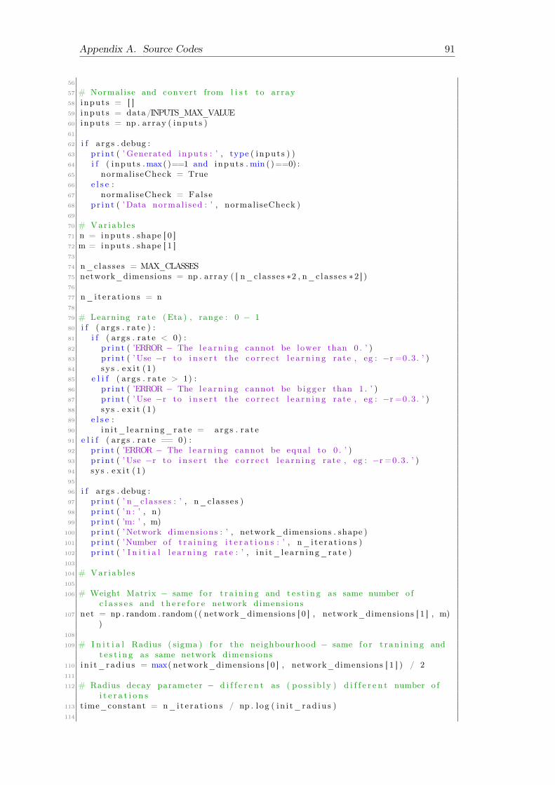
Appendix A. Source Codes 91

56

57 # Normalise and convert from l i s t to array58 inputs = [ ]59 inputs = data/INPUTS_MAX_VALUE60 inputs = np . array ( inputs )61

62 i f a rgs . debug :63 pr in t ( ’ Generated inputs : ’ , type ( inputs ) )64 i f ( inputs .max( )==1 and inputs . min ( )==0) :65 normaliseCheck = True66 e l s e :67 normaliseCheck = False68 pr in t ( ’Data normal i sed : ’ , normaliseCheck )69

70 # Var iab l e s71 n = inputs . shape [ 0 ]72 m = inputs . shape [ 1 ]73

74 n_classes = MAX_CLASSES75 network_dimensions = np . array ( [ n_c lasses ∗2 , n_classes ∗2 ] )76

77 n_i t e ra t i on s = n78

79 # Learning ra t e (Eta ) , range : 0 − 180 i f ( a rgs . r a t e ) :81 i f ( a rgs . r a t e < 0) :82 pr in t ( ’ERROR − The l e a rn i ng cannot be lower than 0 . ’ )83 pr in t ( ’Use −r to i n s e r t the c o r r e c t l e a rn i ng rate , eg : −r =0.3 . ’ )84 sys . e x i t (1 )85 e l i f ( a rgs . r a t e > 1) :86 pr in t ( ’ERROR − The l e a rn i ng cannot be b igge r than 1 . ’ )87 pr in t ( ’Use −r to i n s e r t the c o r r e c t l e a rn i ng rate , eg : −r =0.3 . ’ )88 sys . e x i t (1 )89 e l s e :90 i n i t_ l ea rn ing_rate = args . r a t e91 e l i f ( a rgs . r a t e == 0) :92 pr in t ( ’ERROR − The l e a rn i ng cannot be equal to 0 . ’ )93 pr in t ( ’Use −r to i n s e r t the c o r r e c t l e a rn i ng rate , eg : −r =0.3 . ’ )94 sys . e x i t (1 )95

96 i f a rgs . debug :97 pr in t ( ’ n_c lasses : ’ , n_c lasses )98 pr in t ( ’n : ’ , n )99 pr in t ( ’m: ’ , m)

100 pr in t ( ’ Network dimensions : ’ , network_dimensions . shape )101 pr in t ( ’Number o f t r a i n i n g i t e r a t i o n s : ’ , n_ i t e ra t i on s )102 pr in t ( ’ I n i t i a l l e a rn i ng ra t e : ’ , i n i t_ l ea rn ing_rate )103

104 # Var iab l e s105

106 # Weight Matrix − same f o r t r a i n i n g and t e s t i n g as same number o fc l a s s e s and t h e r e f o r e network dimensions

107 net = np . random . random ( ( network_dimensions [ 0 ] , network_dimensions [ 1 ] , m))

108

109 # I n i t i a l Radius ( sigma ) f o r the neighbourhood − same f o r t r an in i ng andt e s t i n g as same network dimensions

110 i n i t_rad iu s = max( network_dimensions [ 0 ] , network_dimensions [ 1 ] ) / 2111

112 # Radius decay parameter − d i f f e r e n t as ( po s s i b l y ) d i f f e r e n t number o fi t e r a t i o n s

113 time_constant = n_i t e ra t i on s / np . l og ( i n i t_rad iu s )114

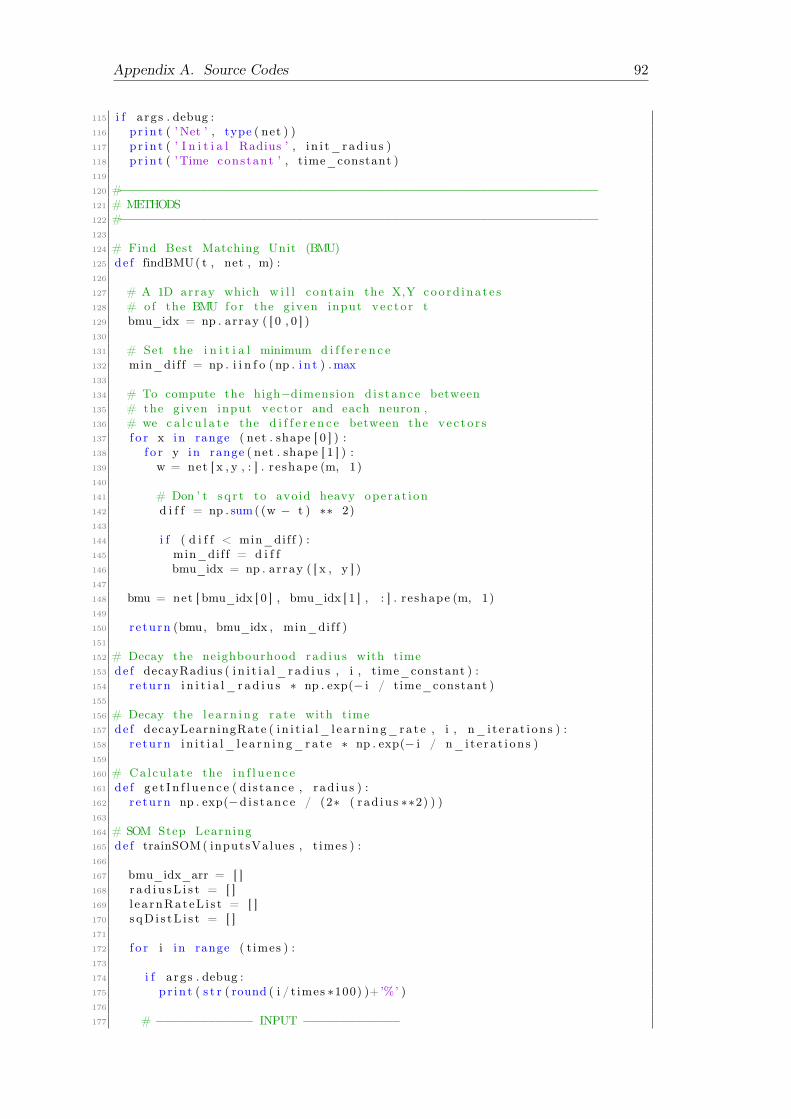
Appendix A. Source Codes 92

115 i f a rgs . debug :116 pr in t ( ’Net ’ , type ( net ) )117 pr in t ( ’ I n i t i a l Radius ’ , i n i t_rad iu s )118 pr in t ( ’Time constant ’ , t ime_constant )119

120 #−−−−−−−−−−−−−−−−−−−−−−−−−−−−−−−−−−−−−−−−−−−−−−−−−−−−−−−−−−−−−−−−−121 # METHODS122 #−−−−−−−−−−−−−−−−−−−−−−−−−−−−−−−−−−−−−−−−−−−−−−−−−−−−−−−−−−−−−−−−−123

124 # Find Best Matching Unit (BMU)125 de f findBMU( t , net , m) :126

127 # A 1D array which w i l l conta in the X,Y coo rd ina t e s128 # of the BMU fo r the g iven input vec to r t129 bmu_idx = np . array ( [ 0 , 0 ] )130

131 # Set the i n i t i a l minimum d i f f e r e n c e132 min_diff = np . i i n f o (np . i n t ) .max133

134 # To compute the high−dimension d i s t ance between135 # the given input vec to r and each neuron ,136 # we c a l c u l a t e the d i f f e r e n c e between the ve c to r s137 f o r x in range ( net . shape [ 0 ] ) :138 f o r y in range ( net . shape [ 1 ] ) :139 w = net [ x , y , : ] . reshape (m, 1)140

141 # Don ’ t sq r t to avoid heavy operat i on142 d i f f = np . sum( (w − t ) ∗∗ 2)143

144 i f ( d i f f < min_diff ) :145 min_diff = d i f f146 bmu_idx = np . array ( [ x , y ] )147

148 bmu = net [ bmu_idx [ 0 ] , bmu_idx [ 1 ] , : ] . reshape (m, 1)149

150 re turn (bmu, bmu_idx , min_diff )151

152 # Decay the neighbourhood rad iu s with time153 de f decayRadius ( i n i t i a l_ r ad i u s , i , t ime_constant ) :154 re turn i n i t i a l_ r a d i u s ∗ np . exp(− i / time_constant )155

156 # Decay the l e a rn i ng ra t e with time157 de f decayLearningRate ( i n i t i a l_ l e a rn i ng_ra t e , i , n_ i t e ra t i on s ) :158 re turn i n i t i a l_ l e a r n i n g_ra t e ∗ np . exp(− i / n_i t e ra t i on s )159

160 # Calcu la te the i n f l u e n c e161 de f g e t I n f l u en c e ( d i s tance , rad iu s ) :162 re turn np . exp(−d i s t anc e / (2∗ ( rad iu s ∗∗2) ) )163

164 # SOM Step Learning165 de f trainSOM( inputsValues , t imes ) :166

167 bmu_idx_arr = [ ]168 r ad i u sL i s t = [ ]169 l e a rnRateL i s t = [ ]170 s qD i s tL i s t = [ ]171

172 f o r i in range ( t imes ) :173

174 i f a rgs . debug :175 pr in t ( s t r ( round ( i / t imes ∗100) )+’%’ )176

177 # −−−−−−−−−−−−− INPUT −−−−−−−−−−−−−

Appendix A. Source Codes 93

178 # 1. S e l e c t a input weight vec to r at each step179

180 # This can be random , however s i n c e we ’ re us ing so r t ed inputs , we ’ re181 # proceed ing in a l i n e a r manner through a l l nodes f o r sake o f

c l a r i t y182 t = inputsValues [ i , : ] . reshape (np . array ( [m, 1 ] ) )183

184 # −−−−−−−−−−−−− BMU −−−−−−−−−−−−−185 # 2. Find the chosen input vec to r ’ s BMU at each step186 #bmu, bmu_idx = findBMU( t , net , m)187 bmu, bmu_idx , d i s t = findBMU( t , net , m)188

189 bmu_idx_arr . append (bmu_idx)190 s qD i s tL i s t . append ( d i s t )191

192 # −−−−−−−−−−−−− DECAY −−−−−−−−−−−−−193 # 3. Determine t o p o l o g i c a l neighbourhood f o r each step194 r = decayRadius ( in i t_rad ius , i , t ime_constant )195 l = decayLearningRate ( in i t_learn ing_rate , i , t imes )196

197 r ad i u sL i s t . append ( r )198 l e a rnRateL i s t . append ( l )199

200 # −−−−−−−−−−−−− UPDATE −−−−−−−−−−−−−201 # 4. Repeat f o r a l l nodes in the ∗BMU neighbourhood∗202 f o r x in range ( net . shape [ 0 ] ) :203 f o r y in range ( net . shape [ 1 ] ) :204

205 # Find weight vec to r206 w = net [ x , y , : ] . reshape (m, 1)207 #wList . append (w)208

209 # Get the 2−D di s t anc e ( not Eucl idean as no sq r t )210 w_dist = np . sum( ( np . array ( [ x , y ] ) − bmu_idx) ∗∗ 2)211 #wDistList . append (w_dist )212

213 # I f the d i s t ance i s with in the cur rent neighbourhood rad iu s214 i f w_dist <= r ∗∗2 :215

216 # Calcu la te the degree o f i n f l u e n c e ( based on the 2−D di s t anc e)

217 i n f l u e n c e = ge t I n f l u en c e (w_dist , r )218

219 # Update weight :220 # new w = old w + ( l e a rn i ng ra t e ∗ i n f l u e n c e ∗ de l t a )221 # de l t a = input vec to r t − o ld w222 new_w = w + ( l ∗ i n f l u e n c e ∗ ( t − w) )223 #new_wList . append (new_w)224

225 # Update net with new weight226 net [ x , y , : ] = new_w. reshape (1 , m)227

228 # Every 100 i t e r a t i o n s we c a l l f o r a SOM to be made to view229 #i f ( i >0 and i%100==0) :230 # bmu_interim_arr = np . array (bmu_idx_arr )231 # makeSOM(bmu_interim_arr , l ab e l s , [ ] , [ ] )232

233 # Convert to NumPy array234 bmu_idx_arr = np . array (bmu_idx_arr )235

236 #np . savetxt ( ( save_path+’%s ’%timeStamped ( )+’_%s ’%n_classes+’ c l a s s e s ’+ ’_%s ’% in i t_ l ea rn ing_rate+’ ra t e ’+ ’_%s ’%chosen_inputs_per_class+’ inputs’+ ’ . csv ’ ) , bmu_idx_arr , fmt=’%d ’ , d e l im i t e r = ’ , ’ )

Appendix A. Source Codes 94

237 #np . savetxt ( ( save_path+’Net_%s ’%timeStamped ( ) + ’. txt ’ ) , net , fmt=’%d ’ )238

239 re turn (bmu_idx_arr , r ad iu sL i s t , l ea rnRateL i s t , s qD i s tL i s t )240

241

242 de f makeSOM(bmu_idx_arr ) :243

244 plotVector = np . z e ro s ( ( n , 5 ) )245 x_coords = [ ]246 y_coords = [ ]247

248 x_coords = np . random . rand int (0 , network_dimensions [ 0 ] ,INPUTS_PER_CLASS)

249 y_coords = np . random . rand int (0 , network_dimensions [ 0 ] ,INPUTS_PER_CLASS)

250

251 x_coords = np . array ( x_coords )252 y_coords = np . array ( y_coords )253

254 # plotVector Format : [X, Y, R, G, B]255 # Coordinates and co l ou r s in a s i n g l e vec to r256

257 # In s e r t t r a i n i n g va lue s258 f o r i in range (n) :259 # X, Ys − Coordinates with added no i s e260 plotVector [ i ] [ 0 ] = bmu_idx_arr [ i ] [ 0 ]261 plotVector [ i ] [ 1 ] = bmu_idx_arr [ i ] [ 1 ]262

263 # R,G, Bs − Color each po int accord ing to c l a s s264 plotVector [ i ] [ 2 ] = inputs [ i ] [ 0 ]265 plotVector [ i ] [ 3 ] = inputs [ i ] [ 1 ]266 plotVector [ i ] [ 4 ] = inputs [ i ] [ 2 ]267

268 # Generate no i s e f o r each po int269 i f ( p lo tVector . shape [ 0 ] > 0) :270 a_x = −0.4271 a_y = −0.4272 b_x = 0.4273 b_y = 0.4274

275 noise_x = (b_x−a_x) ∗ np . random . rand ( p lotVector . shape [ 0 ] , 1) + a_x276 noise_y = (b_y−a_y) ∗ np . random . rand ( p lotVector . shape [ 0 ] , 1) + a_y277

278 zPlot = np . array ( p lotVector [ : , 2 : 5 ] )279

280 # With no i s e281 xPlotNoise = np . add ( p lotVector [ : , 0 ] , noise_x [ : , 0 ] )282 yPlotNoise = np . add ( p lotVector [ : , 1 ] , noise_y [ : , 0 ] )283

284 x_coordsNoise = np . add ( x_coords [ : ] , noise_x [ : , 0 ] )285 y_coordsNoise = np . add ( y_coords [ : ] , noise_y [ : , 0 ] )286

287 # Witout no i s e288 xPlot = plotVector [ : , 0 ]289 yPlot = plotVector [ : , 1 ]290

291 i f ( a rgs . debug ) :292 pr in t ( ’ Rate : ’ , i n i t_ l ea rn ing_rate )293 pr in t ( ’ x : ’ , xPlot . shape )294 pr in t ( ’ y : ’ , yPlot . shape )295 pr in t ( ’ z : ’ , zPlot . shape )296 pr in t ( ’BMUs: ’ , bmu_idx_arr . shape )297 pr in t ( zPlot [ 0 ] )

Appendix A. Source Codes 95

298

299 # Plot S c a t t e r p l o t300 p l o t S i z e = ( n_classes ∗ 2)301 f i g S i z e = 5.91302 p l t . f i g u r e ( )303

304 # Plot nodes305 p l t . s c a t t e r ( x_coords , y_coords , s=20, f a c e c o l o r=zPlot )306 p l t . t i t l e ( s t r (n)+’ Inputs unsorted without no i s e ’ )307 p l t . show ( )308

309 # Plot nodes with no i s e310 p l t . s c a t t e r ( x_coordsNoise , y_coordsNoise , s=20, f a c e c o l o r=zPlot )311 p l t . t i t l e ( s t r (n)+’ Inputs unsorted with no i s e ’ )312 p l t . show ( )313

314 # Plot data without no i s e315 p l t . s c a t t e r ( xPlot , yPlot , s=20, marker=’ o ’ , f a c e c o l o r=zPlot )316 p l t . t i t l e ( s t r (n)+’ Inputs so r t ed without no i s e ’ )317 p l t . show ( )318

319 # Plot data with no i s e320 p l t . s c a t t e r ( xPlotNoise , yPlotNoise , s=20, marker=’ o ’ , f a c e c o l o r=zPlot )321 p l t . t i t l e ( s t r (n)+’ Inputs so r t ed with no i s e ’ )322 p l t . show ( )323

324 # Legend325 #fo r i in range (10) :326 # pl t . s c a t t e r ( i , 1 , s=20, f a c e c o l o r=zPlot [ i ] )327

328 #fo r i in range (n) :329 # pl t . t ex t ( xPlot [ 0 ] , yPlot [ 1 ] , l a b e l s [ i ] , ha=’ cente r ’ , va=’ cente r ’ )330

331 #pl t . l egend ( handles=[n ] )332

333 #pl t . ax i s ( ’ o f f ’ )334

335 # Export as CSV336 unClustered = np . z e r o s ( ( n , 5 ) )337 unClusteredNoise = np . z e ro s ( ( n , 5 ) )338 c l u s t e r e d = np . z e r o s ( ( n , 5 ) )339 c l u s t e r edNo i s e = np . z e ro s ( ( n , 5 ) )340

341 unClustered [ : , 0 ] = x_coords [ : ]342 unClustered [ : , 1 ] = y_coords [ : ]343 unClustered [ : , 2 : 5 ] = data [ : ]344

345 unClusteredNoise [ : , 0 ] = x_coordsNoise [ : ]346 unClusteredNoise [ : , 1 ] = y_coordsNoise [ : ]347 unClusteredNoise [ : , 2 : 5 ] = data [ : ]348

349 c l u s t e r e d [ : , 0 ] = xPlot [ : ]350 c l u s t e r e d [ : , 1 ] = yPlot [ : ]351 c l u s t e r e d [ : , 2 : 5 ] = data [ : ]352

353 c l u s t e r edNo i s e [ : , 0 ] = xPlotNoise [ : ]354 c l u s t e r edNo i s e [ : , 1 ] = yPlotNoise [ : ]355 c l u s t e r edNo i s e [ : , 2 : 5 ] = data [ : ]356

357 np . savetxt ( ( ’ s t a t i c /data/RGB/RGBUnsorted . csv ’ ) , unClustered , fmt=’%d ’ ,d e l im i t e r=’ , ’ , comments=’ ’ , header=’xRGB,yRGB,R,G,B ’ )

358 np . savetxt ( ( ’ s t a t i c /data/RGB/RGBUnsortedNoise . csv ’ ) , unClusteredNoise ,fmt=’%.3 f ’ , d e l im i t e r=’ , ’ , comments=’ ’ , header=’xRGB,yRGB,R,G,B ’ )

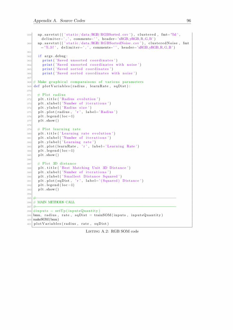
Appendix A. Source Codes 96

359 np . savetxt ( ( ’ s t a t i c /data/RGB/RGBSorted . csv ’ ) , c l u s t e r ed , fmt=’%d ’ ,d e l im i t e r=’ , ’ , comments=’ ’ , header=’xRGB,yRGB,R,G,B ’ )

360 np . savetxt ( ( ’ s t a t i c /data/RGB/RGBSortedNoise . csv ’ ) , c l u s t e r edNo i s e , fmt=’%.3 f ’ , d e l im i t e r=’ , ’ , comments=’ ’ , header=’xRGB,yRGB,R,G,B ’ )

361

362 i f a rgs . debug :363 pr in t ( ’ Saved unsorted coo rd ina t e s ’ )364 pr in t ( ’ Saved unsorted coo rd ina t e s with no i s e ’ )365 pr in t ( ’ Saved so r t ed coo rd ina t e s ’ )366 pr in t ( ’ Saved so r t ed coo rd ina t e s with no i s e ’ )367

368 # Make g raph i c a l comparaisons o f va r i ous parameters369 de f p l o tVa r i ab l e s ( radius , learnRate , sqDis t ) :370

371 # Plot rad iu s372 p l t . t i t l e ( ’ Radius evo lu t i on ’ )373 p l t . x l ab e l ( ’Number o f i t e r a t i o n s ’ )374 p l t . y l ab e l ( ’ Radius s i z e ’ )375 p l t . p l o t ( radius , ’ r ’ , l a b e l=’ Radius ’ )376 p l t . l egend ( l o c=1)377 p l t . show ( )378

379 # Plot l e a rn i ng ra t e380 p l t . t i t l e ( ’ Learning ra t e evo lu t i on ’ )381 p l t . x l ab e l ( ’Number o f i t e r a t i o n s ’ )382 p l t . y l ab e l ( ’ Learning ra t e ’ )383 p l t . p l o t ( learnRate , ’ r ’ , l a b e l=’ Learning Rate ’ )384 p l t . l egend ( l o c=1)385 p l t . show ( )386

387 # Plot 3D d i s t anc e388 p l t . t i t l e ( ’ Best Matching Unit 3D Distance ’ )389 p l t . x l ab e l ( ’Number o f i t e r a t i o n s ’ )390 p l t . y l ab e l ( ’ Smal l e s t Distance Squared ’ )391 p l t . p l o t ( sqDist , ’ r ’ , l a b e l=’ ( Squared ) Distance ’ )392 p l t . l egend ( l o c=1)393 p l t . show ( )394

395 #−−−−−−−−−−−−−−−−−−−−−−−−−−−−−−−−−−−−−−−−−−−−−−−−−−−−−−−−−−−−−−−−−396 # MAIN METHODS CALL397 #−−−−−−−−−−−−−−−−−−−−−−−−−−−−−−−−−−−−−−−−−−−−−−−−−−−−−−−−−−−−−−−−−398 #inputs = setUp ( inputsQuant ity )399 bmu, radius , rate , sqDis t = trainSOM( inputs , inputsQuant ity )400 makeSOM(bmu)401 p l o tVa r i ab l e s ( radius , rate , sqDis t )

Listing A.2: RGB SOM code

Appendix A. Source Codes 97

A.3 Iris.py

1 # Name : Eklavya SARKAR,2 # ID :201135564 ,3 # Username : u5es24

5 # We’ re us ing the I r i s datase t to t r a i n an ANN6 import argparse7 import sys8 import pandas as pd9 import numpy as np

10 import matp lo t l i b . pyplot as p l t11 from matp lo t l i b . l i n e s import Line2D12

13 #−−−−−−−−−−−−−−−−−−−−−−−−−−−−−−−−−−−−−−−−−−−−−−−−−−−−−−−−−−−−−−−−−14 # CONFIG15 #−−−−−−−−−−−−−−−−−−−−−−−−−−−−−−−−−−−−−−−−−−−−−−−−−−−−−−−−−−−−−−−−−16

17 # Argument Parser f o r debugging18 par s e r = argparse . ArgumentParser ( d e s c r i p t i o n=’Make a 2D map o f a

mult id imens iona l input ’ )19 par s e r . add_argument ( ’−d ’ , ’−−debug ’ , a c t i on=’ store_true ’ , d e f au l t=False ,

he lp=’ Pr int debug messages to s t d e r r ’ )20 par s e r . add_argument ( ’−r ’ , ’−−r a t e ’ , type=f l o a t , a c t i on=’ s t o r e ’ , d e f au l t

=0.3 , he lp=’ Choose l e a rn i ng ra t e ( range : 0−1) ’ )21 args = par s e r . parse_args ( )22

23 #−−−−−−−−−−−−−−−−−−−−−−−−−−−−−−−−−−−−−−−−−−−−−−−−−−−−−−−−−−−−−−−−−24 # SET−UP25 #−−−−−−−−−−−−−−−−−−−−−−−−−−−−−−−−−−−−−−−−−−−−−−−−−−−−−−−−−−−−−−−−−26

27 # Constants28 # ======== DO NOT CHANGE ========|29 INPUTS_MAX_VALUE = 7.9 #|30 MAX_CLASSES = 3 #|31 MAX_INPUTS_PER_CLASS = 50 #|32 # =========DO NOT CHANGE ========|33

34 chosen_inputs_per_class = 5035 n_classes = MAX_CLASSES36

37 # Learning ra t e (Eta ) , range : 0 − 138 i f ( a rgs . r a t e ) :39 i f ( a rgs . r a t e < 0) :40 pr in t ( ’ERROR − The l e a rn i ng cannot be lower than 0 . ’ )41 pr in t ( ’Use −r to i n s e r t the c o r r e c t l e a rn i ng rate , eg : −r =0.3 . ’ )42 sys . e x i t (1 )43 e l i f ( a rgs . r a t e > 1) :44 pr in t ( ’ERROR − The l e a rn i ng cannot be b igge r than 1 . ’ )45 pr in t ( ’Use −r to i n s e r t the c o r r e c t l e a rn i ng rate , eg : −r =0.3 . ’ )46 sys . e x i t (1 )47 e l s e :48 i n i t_ l ea rn ing_rate = args . r a t e49 e l i f ( a rgs . r a t e == 0) :50 pr in t ( ’ERROR − The l e a rn i ng cannot be equal to 0 . ’ )51 pr in t ( ’Use −r to i n s e r t the c o r r e c t l e a rn i ng rate , eg : −r =0.3 . ’ )52 sys . e x i t (1 )53

54 i f a rgs . debug :55 pr in t ( "Debug mode ON" )56 pr in t ( ’ Loading input f i l e s . . . ’ )57

Appendix A. Source Codes 98

58 # Raw Data59 #data_path = ’ s t a t i c /data/ I r i s / I r i sO r i g i n a l . csv ’60 data_path = ’ http :// a rch ive . i c s . uc i . edu/ml/machine−l e a rn ing−databases /

i r i s / i r i s . data ’61 data = pd . read_csv ( data_path , encoding=’ utf−8 ’ , header=None )62

63 # Add Column names64 a t t r i b u t e s = [ " sepa l_length " , " sepal_width" , " peta l_length " , "

petal_width" , " c l a s s " ]65 data . columns = a t t r i b u t e s66

67 # Looping68 l o opSta r t = 069 loopEnd = MAX_CLASSES∗MAX_INPUTS_PER_CLASS70 l a b e l s = [ ]71 inputs = [ ]72

73 f o r i in range ( loopStart , loopEnd ,MAX_INPUTS_PER_CLASS) :74 f o r j in range ( chosen_inputs_per_class ) :75 inputs . append ( data . i l o c [ i+j ] [ 0 : 4 ] /INPUTS_MAX_VALUE) # Append

normal i sed value76 l a b e l s . append ( data . i l o c [ i ] [ 4 ] )77

78 # Put l a b e l s in s epe ra t e NumPy array79 #l a b e l s = np . array ( data [ ’ c l a s s ’ ] )80 l a b e l s = np . array ( l a b e l s )81

82 # Put inputs in a a s epe ra t e NumPy Array , whi l e norma l i s ing i t83 #inputs = np . array ( data [ [ " sepa l_length " , " sepal_width " , " peta l_length " ,

"petal_width " ] ] / inputs .max( ) )84 inputs = np . array ( inputs )85

86 i f a rgs . debug :87 i f ( inputs .max( )==1 and inputs . min ( )==0) :88 normaliseCheck = True89 e l s e :90 normaliseCheck = False91

92 pr in t ( ’ Loaded inputs : ’ , type ( inputs ) )93 pr in t ( ’ Loaded l a b e l s : ’ , type ( l a b e l s ) )94 pr in t ( ’Data normal i sed : ’ , normaliseCheck )95

96 # Var iab l e s97 n = inputs . shape [ 0 ]98 m = inputs . shape [ 1 ]99

100 network_dimensions = np . array ( [ n_c lasses ∗2 , n_classes ∗2 ] )101 n_i t e ra t i on s = n102

103 i f a rgs . debug :104 pr in t ( ’ n_c lasses : ’ , n_c lasses )105 pr in t ( ’n : ’ , n )106 pr in t ( ’m: ’ , m)107 pr in t ( ’ Network dimensions : ’ , network_dimensions . shape )108 pr in t ( ’Number o f t r a i n i n g i t e r a t i o n s : ’ , n_ i t e ra t i on s )109 pr in t ( ’ I n i t i a l l e a rn i ng ra t e : ’ , i n i t_ l ea rn ing_rate )110 pr in t ( ’ Inputs per c l a s s : ’ , chosen_inputs_per_class )111

112

113 # Weight Matrix − same f o r t r a i n i n g and t e s t i n g as same number o fc l a s s e s and t h e r e f o r e network dimensions

114 net = np . random . random ( ( network_dimensions [ 0 ] , network_dimensions [ 1 ] , m))

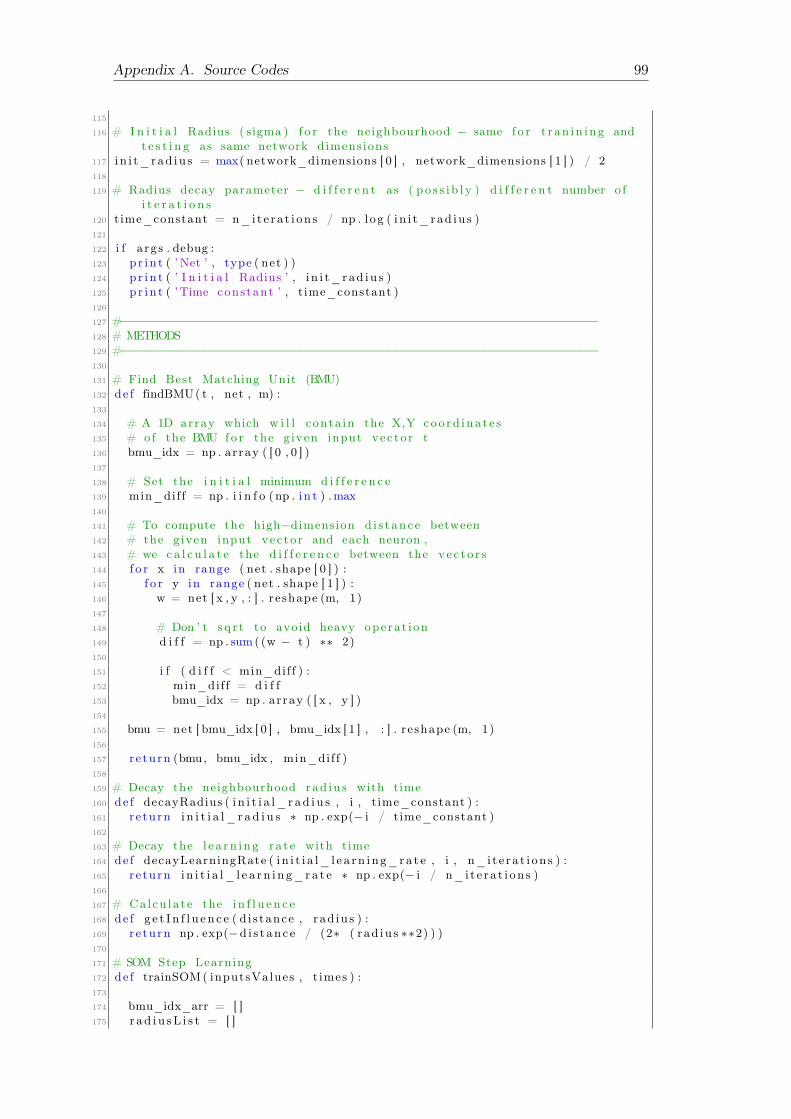
Appendix A. Source Codes 99

115

116 # I n i t i a l Radius ( sigma ) f o r the neighbourhood − same f o r t r an in i ng andt e s t i n g as same network dimensions

117 i n i t_rad iu s = max( network_dimensions [ 0 ] , network_dimensions [ 1 ] ) / 2118

119 # Radius decay parameter − d i f f e r e n t as ( po s s i b l y ) d i f f e r e n t number o fi t e r a t i o n s

120 time_constant = n_i t e ra t i on s / np . l og ( i n i t_rad iu s )121

122 i f a rgs . debug :123 pr in t ( ’Net ’ , type ( net ) )124 pr in t ( ’ I n i t i a l Radius ’ , i n i t_rad iu s )125 pr in t ( ’Time constant ’ , t ime_constant )126

127 #−−−−−−−−−−−−−−−−−−−−−−−−−−−−−−−−−−−−−−−−−−−−−−−−−−−−−−−−−−−−−−−−−128 # METHODS129 #−−−−−−−−−−−−−−−−−−−−−−−−−−−−−−−−−−−−−−−−−−−−−−−−−−−−−−−−−−−−−−−−−130

131 # Find Best Matching Unit (BMU)132 de f findBMU( t , net , m) :133

134 # A 1D array which w i l l conta in the X,Y coo rd ina t e s135 # of the BMU fo r the g iven input vec to r t136 bmu_idx = np . array ( [ 0 , 0 ] )137

138 # Set the i n i t i a l minimum d i f f e r e n c e139 min_diff = np . i i n f o (np . i n t ) .max140

141 # To compute the high−dimension d i s t ance between142 # the given input vec to r and each neuron ,143 # we c a l c u l a t e the d i f f e r e n c e between the ve c to r s144 f o r x in range ( net . shape [ 0 ] ) :145 f o r y in range ( net . shape [ 1 ] ) :146 w = net [ x , y , : ] . reshape (m, 1)147

148 # Don ’ t sq r t to avoid heavy operat i on149 d i f f = np . sum( (w − t ) ∗∗ 2)150

151 i f ( d i f f < min_diff ) :152 min_diff = d i f f153 bmu_idx = np . array ( [ x , y ] )154

155 bmu = net [ bmu_idx [ 0 ] , bmu_idx [ 1 ] , : ] . reshape (m, 1)156

157 re turn (bmu, bmu_idx , min_diff )158

159 # Decay the neighbourhood rad iu s with time160 de f decayRadius ( i n i t i a l_ r ad i u s , i , t ime_constant ) :161 re turn i n i t i a l_ r a d i u s ∗ np . exp(− i / time_constant )162

163 # Decay the l e a rn i ng ra t e with time164 de f decayLearningRate ( i n i t i a l_ l e a rn i ng_ra t e , i , n_ i t e ra t i on s ) :165 re turn i n i t i a l_ l e a r n i n g_ra t e ∗ np . exp(− i / n_i t e ra t i on s )166

167 # Calcu la te the i n f l u e n c e168 de f g e t I n f l u en c e ( d i s tance , rad iu s ) :169 re turn np . exp(−d i s t anc e / (2∗ ( rad iu s ∗∗2) ) )170

171 # SOM Step Learning172 de f trainSOM( inputsValues , t imes ) :173

174 bmu_idx_arr = [ ]175 r ad i u sL i s t = [ ]

Appendix A. Source Codes 100

176 l e a rnRateL i s t = [ ]177 s qD i s tL i s t = [ ]178

179 f o r i in range ( t imes ) :180

181 i f a rgs . debug :182 pr in t ( s t r ( round ( i / t imes ∗100) )+’%’ )183

184 # −−−−−−−−−−−−− INPUT −−−−−−−−−−−−−185 # 1. S e l e c t a input weight vec to r at each step186

187 # This can be random , however s i n c e we ’ re us ing so r t ed inputs , we ’ re188 # proceed ing in a l i n e a r manner through a l l nodes f o r sake o f

c l a r i t y189 t = inputsValues [ i , : ] . reshape (np . array ( [m, 1 ] ) )190

191 # −−−−−−−−−−−−− BMU −−−−−−−−−−−−−192 # 2. Find the chosen input vec to r ’ s BMU at each step193 #bmu, bmu_idx = findBMU( t , net , m)194 bmu, bmu_idx , d i s t = findBMU( t , net , m)195

196 bmu_idx_arr . append (bmu_idx)197 s qD i s tL i s t . append ( d i s t )198

199 # −−−−−−−−−−−−− DECAY −−−−−−−−−−−−−200 # 3. Determine t o p o l o g i c a l neighbourhood f o r each step201 r = decayRadius ( in i t_rad ius , i , t ime_constant )202 l = decayLearningRate ( in i t_learn ing_rate , i , t imes )203

204 r ad i u sL i s t . append ( r )205 l e a rnRateL i s t . append ( l )206

207 # −−−−−−−−−−−−− UPDATE −−−−−−−−−−−−−208 # 4. Repeat f o r a l l nodes in the ∗BMU neighbourhood∗209 f o r x in range ( net . shape [ 0 ] ) :210 f o r y in range ( net . shape [ 1 ] ) :211

212 # Find weight vec to r213 w = net [ x , y , : ] . reshape (m, 1)214 #wList . append (w)215

216 # Get the 2−D di s t anc e ( not Eucl idean as no sq r t )217 w_dist = np . sum( ( np . array ( [ x , y ] ) − bmu_idx) ∗∗ 2)218 #wDistList . append (w_dist )219

220 # I f the d i s t ance i s with in the cur rent neighbourhood rad iu s221 i f w_dist <= r ∗∗2 :222

223 # Calcu la te the degree o f i n f l u e n c e ( based on the 2−D di s t anc e)

224 i n f l u e n c e = ge t I n f l u en c e (w_dist , r )225

226 # Update weight :227 # new w = old w + ( l e a rn i ng ra t e ∗ i n f l u e n c e ∗ de l t a )228 # de l t a = input vec to r t − o ld w229 new_w = w + ( l ∗ i n f l u e n c e ∗ ( t − w) )230 #new_wList . append (new_w)231

232 # Update net with new weight233 net [ x , y , : ] = new_w. reshape (1 , m)234

235 # Every 100 i t e r a t i o n s we c a l l f o r a SOM to be made to view236 #i f ( i >0 and i%100==0) :

Appendix A. Source Codes 101

237 # bmu_interim_arr = np . array (bmu_idx_arr )238 # makeSOM(bmu_interim_arr , l ab e l s , [ ] , [ ] )239

240 # Convert to NumPy array241 bmu_idx_arr = np . array (bmu_idx_arr )242

243 #np . savetxt ( ( save_path+’%s ’%timeStamped ( )+’_%s ’%n_classes+’ c l a s s e s ’+ ’_%s ’% in i t_ l ea rn ing_rate+’ ra t e ’+ ’_%s ’%chosen_inputs_per_class+’ inputs’+ ’ . csv ’ ) , bmu_idx_arr , fmt=’%d ’ , d e l im i t e r = ’ , ’ )

244 #np . savetxt ( ( save_path+’Net_%s ’%timeStamped ( ) + ’. txt ’ ) , net , fmt=’%d ’ )245

246 re turn (bmu_idx_arr , r ad iu sL i s t , l ea rnRateL i s t , s qD i s tL i s t )247

248 de f makeSOM(bmu_idx_arr ) :249

250 plotVector = np . z e ro s ( ( n , 5 ) )251

252 x_coords = [ ]253 y_coords = [ ]254

255 x_coords = np . random . rand int (0 , 6 , chosen_inputs_per_class ∗ n_classes )256 y_coords = np . random . rand int (0 , 6 , chosen_inputs_per_class ∗ n_classes )257

258 x_coords = np . array ( x_coords )259 y_coords = np . array ( y_coords )260

261 # plotVector Format : [X, Y, R, G, B]262 # Coordinates and co l ou r s in a s i n g l e vec to r263

264 # In s e r t t r a i n i n g va lue s265 f o r i in range (n) :266 # X, Ys − Coordinates with added no i s e267 plotVector [ i ] [ 0 ] = bmu_idx_arr [ i ] [ 0 ]268 plotVector [ i ] [ 1 ] = bmu_idx_arr [ i ] [ 1 ]269

270 # R,G, Bs − Color each po int accord ing to c l a s s271 # RGB Values are normal i sed272 i f ( l a b e l s [ i ]== ’ I r i s −s e t o s a ’ ) :273 plotVector [ i ] [ 2 ] = 1274 plotVector [ i ] [ 3 ] = 0275 plotVector [ i ] [ 4 ] = 0276 e l i f ( l a b e l s [ i ]== ’ I r i s −v e r s i c o l o r ’ ) :277 plotVector [ i ] [ 2 ] = 0278 plotVector [ i ] [ 3 ] = 1279 plotVector [ i ] [ 4 ] = 0280 e l i f ( l a b e l s [ i ]== ’ I r i s −v i r g i n i c a ’ ) :281 plotVector [ i ] [ 2 ] = 0282 plotVector [ i ] [ 3 ] = 0283 plotVector [ i ] [ 4 ] = 1284

285 # Generate no i s e f o r each po int286 i f ( p lo tVector . shape [ 0 ] > 0) :287 a_x = −0.4288 a_y = −0.4289 b_x = 0.4290 b_y = 0.4291

292 noise_x = (b_x−a_x) ∗ np . random . rand ( p lotVector . shape [ 0 ] , 1) + a_x293 noise_y = (b_y−a_y) ∗ np . random . rand ( p lotVector . shape [ 0 ] , 1) + a_y294

295 zPlot = np . array ( p lotVector [ : , 2 : 5 ] )296

297 # With no i s e

Appendix A. Source Codes 102

298 xPlotNoise = np . add ( p lotVector [ : , 0 ] , noise_x [ : , 0 ] )299 yPlotNoise = np . add ( p lotVector [ : , 1 ] , noise_y [ : , 0 ] )300

301 x_coordsNoise = np . add ( x_coords [ : ] , noise_x [ : , 0 ] )302 y_coordsNoise = np . add ( y_coords [ : ] , noise_y [ : , 0 ] )303

304 # Witout no i s e305 xPlot = plotVector [ : , 0 ]306 yPlot = plotVector [ : , 1 ]307

308 i f ( a rgs . debug ) :309 pr in t ( ’ Rate : ’ , i n i t_ l ea rn ing_rate )310 pr in t ( ’ x : ’ , xPlot . shape )311 pr in t ( ’ y : ’ , yPlot . shape )312 pr in t ( ’ z : ’ , zPlot . shape )313 pr in t ( ’BMUs: ’ , bmu_idx_arr . shape )314

315 # Legend316 legend_elements = [ Line2D ( [ 0 ] , [ 0 ] , marker=’ o ’ , c o l o r=’ r ’ , l a b e l=’ I r i s

−s e t o s a ’ , marke r f aceco l o r=’ r ’ , markers i ze=5) ,317 Line2D ( [ 0 ] , [ 0 ] , marker=’ o ’ , c o l o r=’ g ’ , l a b e l=’ I r i s

−v e r s i c o l o r ’ , marke r f aceco l o r=’ g ’ , markers i ze=5) ,318 Line2D ( [ 0 ] , [ 0 ] , marker=’ o ’ , c o l o r=’b ’ , l a b e l=’ I r i s

−v i r g i n i c a ’ , marke r f aceco l o r=’b ’ , markers i ze=5) ]319

320 # Plot S c a t t e r p l o t321 p l o t S i z e = ( n_classes ∗ 2)322 f i g S i z e = 5.91323 p l t . f i g u r e ( )324

325 # Plot nodes326 p l t . s c a t t e r ( x_coords , y_coords , s=20, f a c e c o l o r=zPlot )327 p l t . t i t l e ( s t r (n)+’ Inputs unsorted without no i s e ’ )328 p l t . l egend ( handles=legend_elements , l o c=1)329 p l t . show ( )330

331 # Plot nodes with no i s e332 p l t . s c a t t e r ( x_coordsNoise , y_coordsNoise , s=20, f a c e c o l o r=zPlot )333 p l t . t i t l e ( s t r (n)+’ Inputs unsorted with no i s e ’ )334 p l t . l egend ( handles=legend_elements , l o c=1)335 p l t . show ( )336

337 # Plot data without no i s e338 p l t . s c a t t e r ( xPlot , yPlot , s=20, marker=’ o ’ , f a c e c o l o r=zPlot )339 p l t . t i t l e ( s t r (n)+’ Inputs so r t ed without no i s e ’ )340 p l t . l egend ( handles=legend_elements , l o c=1)341 p l t . show ( )342

343 # Plot data with no i s e344 p l t . s c a t t e r ( xPlotNoise , yPlotNoise , s=20, marker=’ o ’ , f a c e c o l o r=zPlot )345 p l t . t i t l e ( s t r (n)+’ Inputs so r t ed with no i s e ’ )346 p l t . l egend ( handles=legend_elements , l o c=1)347 p l t . show ( )348

349 # Legend350 #fo r i in range (10) :351 # pl t . s c a t t e r ( i , 1 , s=20, f a c e c o l o r=zPlot [ i ] )352

353 #fo r i in range (n) :354 # pl t . t ex t ( xPlot [ 0 ] , yPlot [ 1 ] , l a b e l s [ i ] , ha=’ cente r ’ , va=’ cente r ’ )355

356 #pl t . l egend ( handles=[n ] )357

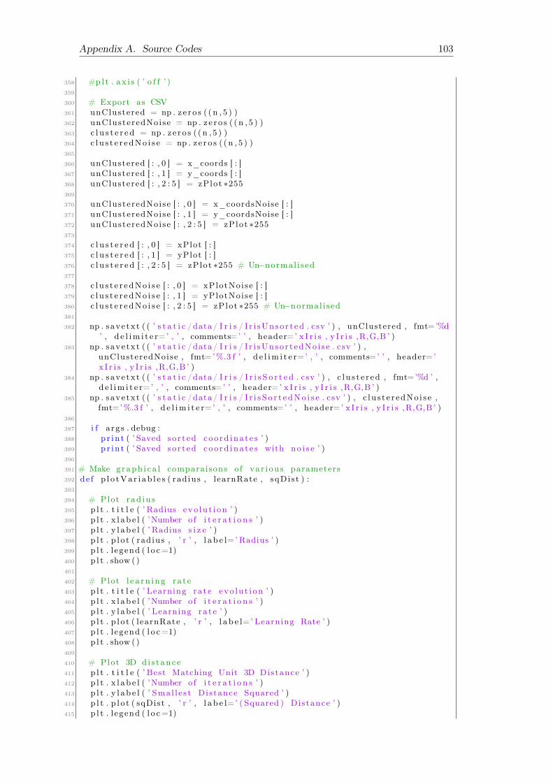
Appendix A. Source Codes 103

358 #pl t . ax i s ( ’ o f f ’ )359

360 # Export as CSV361 unClustered = np . z e r o s ( ( n , 5 ) )362 unClusteredNoise = np . z e ro s ( ( n , 5 ) )363 c l u s t e r e d = np . z e r o s ( ( n , 5 ) )364 c l u s t e r edNo i s e = np . z e ro s ( ( n , 5 ) )365

366 unClustered [ : , 0 ] = x_coords [ : ]367 unClustered [ : , 1 ] = y_coords [ : ]368 unClustered [ : , 2 : 5 ] = zPlot ∗255369

370 unClusteredNoise [ : , 0 ] = x_coordsNoise [ : ]371 unClusteredNoise [ : , 1 ] = y_coordsNoise [ : ]372 unClusteredNoise [ : , 2 : 5 ] = zPlot ∗255373

374 c l u s t e r e d [ : , 0 ] = xPlot [ : ]375 c l u s t e r e d [ : , 1 ] = yPlot [ : ]376 c l u s t e r e d [ : , 2 : 5 ] = zPlot ∗255 # Un−normal i sed377

378 c l u s t e r edNo i s e [ : , 0 ] = xPlotNoise [ : ]379 c l u s t e r edNo i s e [ : , 1 ] = yPlotNoise [ : ]380 c l u s t e r edNo i s e [ : , 2 : 5 ] = zPlot ∗255 # Un−normal i sed381

382 np . savetxt ( ( ’ s t a t i c /data/ I r i s / I r i sUnso r t ed . csv ’ ) , unClustered , fmt=’%d’ , d e l im i t e r=’ , ’ , comments=’ ’ , header=’ x I r i s , y I r i s ,R,G,B ’ )

383 np . savetxt ( ( ’ s t a t i c /data/ I r i s / I r i sUnso r t edNo i s e . csv ’ ) ,unClusteredNoise , fmt=’%.3 f ’ , d e l im i t e r=’ , ’ , comments=’ ’ , header=’x I r i s , y I r i s ,R,G,B ’ )

384 np . savetxt ( ( ’ s t a t i c /data/ I r i s / I r i s S o r t e d . csv ’ ) , c l u s t e r ed , fmt=’%d ’ ,d e l im i t e r=’ , ’ , comments=’ ’ , header=’ x I r i s , y I r i s ,R,G,B ’ )

385 np . savetxt ( ( ’ s t a t i c /data/ I r i s / I r i s S o r t e dNo i s e . csv ’ ) , c l u s t e r edNo i s e ,fmt=’%.3 f ’ , d e l im i t e r=’ , ’ , comments=’ ’ , header=’ x I r i s , y I r i s ,R,G,B ’ )

386

387 i f a rgs . debug :388 pr in t ( ’ Saved so r t ed coo rd ina t e s ’ )389 pr in t ( ’ Saved so r t ed coo rd ina t e s with no i s e ’ )390

391 # Make g raph i c a l comparaisons o f va r i ous parameters392 de f p l o tVa r i ab l e s ( radius , learnRate , sqDis t ) :393

394 # Plot rad iu s395 p l t . t i t l e ( ’ Radius evo lu t i on ’ )396 p l t . x l ab e l ( ’Number o f i t e r a t i o n s ’ )397 p l t . y l ab e l ( ’ Radius s i z e ’ )398 p l t . p l o t ( radius , ’ r ’ , l a b e l=’ Radius ’ )399 p l t . l egend ( l o c=1)400 p l t . show ( )401

402 # Plot l e a rn i ng ra t e403 p l t . t i t l e ( ’ Learning ra t e evo lu t i on ’ )404 p l t . x l ab e l ( ’Number o f i t e r a t i o n s ’ )405 p l t . y l ab e l ( ’ Learning ra t e ’ )406 p l t . p l o t ( learnRate , ’ r ’ , l a b e l=’ Learning Rate ’ )407 p l t . l egend ( l o c=1)408 p l t . show ( )409

410 # Plot 3D d i s t anc e411 p l t . t i t l e ( ’ Best Matching Unit 3D Distance ’ )412 p l t . x l ab e l ( ’Number o f i t e r a t i o n s ’ )413 p l t . y l ab e l ( ’ Smal l e s t Distance Squared ’ )414 p l t . p l o t ( sqDist , ’ r ’ , l a b e l=’ ( Squared ) Distance ’ )415 p l t . l egend ( l o c=1)

Appendix A. Source Codes 104

416 p l t . show ( )417

418 #−−−−−−−−−−−−−−−−−−−−−−−−−−−−−−−−−−−−−−−−−−−−−−−−−−−−−−−−−−−−−−−−−419 # MAIN METHOD CALLS420 #−−−−−−−−−−−−−−−−−−−−−−−−−−−−−−−−−−−−−−−−−−−−−−−−−−−−−−−−−−−−−−−−−421 bmu, radius , rate , sqDis t = trainSOM( inputs , 150)422 makeSOM(bmu)423 p l o tVa r i ab l e s ( radius , rate , sqDis t )

Listing A.3: Iris SOM code

Appendix A. Source Codes 105

A.4 SOM.py

1 # Name : Eklavya SARKAR,2 # ID :201135564 ,3 # Username : u5es24

5 # We’ re us ing so r t ed EMNIST Balanced 47 C la s s e s data , to make a SOM6

7 import argparse8 import sys9 import datet ime

10 import numpy as np11 import pandas as pd12 import matp lo t l i b . pyplot as p l t13

14 # Argument Parser f o r debugging15 par s e r = argparse . ArgumentParser ( d e s c r i p t i o n=’Make a 2D map o f a

mult id imens iona l input ’ )16 par s e r . add_argument ( ’−d ’ , ’−−debug ’ , a c t i on=’ store_true ’ , d e f au l t=False ,

he lp=’ Pr int debug messages to s t d e r r ’ )17 par s e r . add_argument ( ’−t ’ , ’−−type ’ , a c t i on=’ s t o r e ’ , d e f au l t="d" , he lp=’

Choose type o f datase t : l e t t e r s (= l ) , d i g i t s (=d) , or combined(=c ) ’ )18 par s e r . add_argument ( ’−r ’ , ’−−r a t e ’ , type=f l o a t , a c t i on=’ s t o r e ’ , d e f au l t

=0.3 , he lp=’ Choose l e a rn i ng ra t e ( range : 0−1) ’ )19 par s e r . add_argument ( ’−iTr ’ , ’−−inputsTra in ’ , type=int , a c t i on=’ s t o r e ’ ,

d e f au l t =20, he lp=’ Choose number o f t r a i n inputs per c l a s s ( range :0−2400) ’ )

20 par s e r . add_argument ( ’−iTe ’ , ’−−inputsTest ’ , type=int , a c t i on=’ s t o r e ’ ,d e f au l t =20, he lp=’ Choose number o f t e s t inputs per c l a s s ( range :0−400) ’ )

21 args = par s e r . parse_args ( )22

23 #−−−−−−−−−−−−−−−−−−−−−−−−−−−−−−−−−−−−−−−−−−−−−−−−−−−−−−−−−−−−−−−−−24 # CONFIG25 #−−−−−−−−−−−−−−−−−−−−−−−−−−−−−−−−−−−−−−−−−−−−−−−−−−−−−−−−−−−−−−−−−26

27 # Constants28 # ======== DO NOT CHANGE ========|29 INPUTS_MAX_VALUE = 255 #|30 MAX_CLASSES = 47 #|31 MAX_INPUTS_PER_CLASS = 2400 #|32 MAX_TEST_INPUTS_PER_CLASS = 400 #|33 # =========DO NOT CHANGE ========|34

35 # Parameters c on f i gu r e accord ing to g iven arguments36 i f not l en ( vars ( args ) ) > 1 :37 pr in t ( ’ Using d e f au l t va lue s ’ )38

39 # Number o f t r a i n i n g inputs , range : 0 − 240040 i f ( a rgs . inputsTra in ) :41 i f ( a rgs . inputsTra in < 0) :42 pr in t ( ’ERROR − The number o f t r a i n i n g inputs cannot be lower than 0 .

’ )43 pr in t ( ’Use −iTr to i n s e r t a c o r r e c t number o f inputs , eg : −iTr=20. ’ )44 sys . e x i t (1 )45 i f ( a rgs . inputsTra in > 2400) :46 pr in t ( ’ERROR − The number o f t r a i n i n g inputs cannot be h igher than

2400 . ’ )47 pr in t ( ’Use −iTr to i n s e r t a c o r r e c t number o f inputs , eg : −iTr=20. ’ )48 sys . e x i t (1 )49 e l s e :50 chosen_inputs_per_class = args . inputsTra in

Appendix A. Source Codes 106

51

52 e l i f ( a rgs . inputsTra in == 0) :53 pr in t ( ’ERROR − The number o f t r a i n i n g inputs cannot be equal to 0 . ’ )54 pr in t ( ’Use −iTr to i n s e r t a c o r r e c t number o f inputs , eg : −iTr=20. ’ )55 sys . e x i t (1 )56

57 # Number o f t e s t i n g inputs , range : 0 − 240058 i f ( a rgs . inputsTest ) :59 i f ( a rgs . inputsTest < 0) :60 pr in t ( ’ERROR − The number o f t e s t i n g inputs cannot be lower than 0 . ’

)61 pr in t ( ’Use −iTe to i n s e r t a c o r r e c t number o f inputs , eg : −iTe=20. ’ )62 sys . e x i t (1 )63 i f ( a rgs . inputsTest > 2400) :64 pr in t ( ’ERROR − The number o f t e s t i n g inputs cannot be h igher than

2400 . ’ )65 pr in t ( ’Use −iTe to i n s e r t a c o r r e c t number o f inputs , eg : −iTe=20. ’ )66 sys . e x i t (1 )67 e l s e :68 chosen_test_inputs_per_class = args . inputsTest69

70 e l i f ( a rgs . inputsTest == 0) :71 pr in t ( ’ERROR − The number o f t e s t i n g inputs cannot be equal to 0 . ’ )72 pr in t ( ’Use −iTe to i n s e r t a c o r r e c t number o f inputs , eg : −iTe=20. ’ )73 sys . e x i t (1 )74

75 # Learning ra t e (Eta ) , range : 0 − 176 i f ( a rgs . r a t e ) :77 i f ( a rgs . r a t e < 0) :78 pr in t ( ’ERROR − The l e a rn i ng cannot be lower than 0 . ’ )79 pr in t ( ’Use −r to i n s e r t the c o r r e c t l e a rn i ng rate , eg : −r =0.3 . ’ )80 sys . e x i t (1 )81 e l i f ( a rgs . r a t e > 1) :82 pr in t ( ’ERROR − The l e a rn i ng cannot be b igge r than 1 . ’ )83 pr in t ( ’Use −r to i n s e r t the c o r r e c t l e a rn i ng rate , eg : −r =0.3 . ’ )84 sys . e x i t (1 )85 e l s e :86 i n i t_ l ea rn ing_rate = args . r a t e87 e l i f ( a rgs . r a t e == 0) :88 pr in t ( ’ERROR − The l e a rn i ng cannot be equal to 0 . ’ )89 pr in t ( ’Use −r to i n s e r t the c o r r e c t l e a rn i ng rate , eg : −r =0.3 . ’ )90 sys . e x i t (1 )91

92 # Number o f c l a s s e s93 i f ( a rgs . type == ’d ’ ) : # Dig i t s94 n_classes = 1095 e l i f ( a rgs . type == ’ l ’ ) : # Le t t e r s96 n_classes = MAX_CLASSES−1097 e l i f ( a rgs . type == ’ c ’ ) : # Combined98 n_classes = MAX_CLASSES99 e l s e :

100 pr in t ( ’ERROR − I nva l i d c l a s s type . ’ )101 pr in t ( ’Use −t to i n s e r t the c o r r e c t c l a s s type , eg : −t=d . ’ )102 sys . e x i t (1 )103

104 #−−−−−−−−−−−−−−−−−−−−−−−−−−−−−−−−−−−−−−−−−−−−−−−−−−−−−−−−−−−−−−−−−105 # SET−UP106 #−−−−−−−−−−−−−−−−−−−−−−−−−−−−−−−−−−−−−−−−−−−−−−−−−−−−−−−−−−−−−−−−−107

108 i f a rgs . debug :109 pr in t ( "Debug mode ON" )110 pr in t ( ’ Loading input f i l e s . . . ’ )111

Appendix A. Source Codes 107

112 # Inputs ( Sorted inputs o f a l l 47 c l a s s e s )113 #train_inputs_path = ’/ Users / eklavya /Movies/EMNIST_csv/Balanced/Sorted /

SortedTra inInputs . csv ’114 train_inputs_path = ’ http :// c g i . c s c . l i v . ac . uk/~u5es2 /EMNIST/Sorted /Train

. csv ’115 t ra in_inputs = pd . read_csv ( train_inputs_path , encoding=’ utf−8 ’ , header=

None )116

117 #test_inputs_path = ’/ Users / eklavya /Movies/EMNIST_csv/Balanced/ Sorted /SortedTest Inputs . csv ’

118 test_inputs_path = ’ http :// c g i . c s c . l i v . ac . uk/~u5es2 /EMNIST/Sorted /Test .csv ’

119 te s t_inputs = pd . read_csv ( test_inputs_path , encoding=’ utf−8 ’ , header=None )

120

121 i f a rgs . debug :122 pr in t ( ’ Loaded 1/3 f i l e s ’ )123

124 # Labels125 #train_labe ls_path = ’/ Users / eklavya /Movies/EMNIST_csv/Balanced/Sorted /

SortedTra inLabe l s . txt ’126 tra in_labe ls_path = ’ http :// c g i . c s c . l i v . ac . uk/~u5es2 /EMNIST/Sorted /

TrainLabels . txt ’127 t r a i n_ l abe l s = pd . read_csv ( tra in_labels_path , encoding=’ utf−8 ’ , dtype=np

. int8 , header=None )128

129 #test_labe l s_path = ’/ Users / eklavya /Movies/EMNIST_csv/Balanced/ Sorted /SortedTestLabe l s . txt ’

130 test_labe l s_path = ’ http :// c g i . c s c . l i v . ac . uk/~u5es2 /EMNIST/Sorted /TestLabels . txt ’

131 t e s t_ l ab e l s = pd . read_csv ( test_labels_path , encoding=’ utf−8 ’ , dtype=np .int8 , header=None )

132

133 # Drawn input134 # drawn_path = ’/ Users / eklavya /Dropbox/__Liverpool/_390/SourceCode/

EMNIST−Kohonen−SOM/ s t a t i c /data/drawn . csv ’135 # drawn_input = pd . read_csv (drawn_path , encoding=’utf −8 ’ , header=None )136

137 i f a rgs . debug :138 pr in t ( ’ Loaded 2/3 f i l e s ’ )139

140 i f ( a rgs . type == ’d ’ ) :141 colours_path = ’ /Users / eklavya /Dropbox/__Liverpool/_390/SourceCode /10

Colors . csv ’142 save_path = ’ /Users /Eklavya/Movies/EMNIST_csv/Balanced/Runs/ D ig i t s / ’143 e l i f ( a rgs . type == ’ l ’ ) :144 colours_path = ’ /Users / eklavya /Dropbox/__Liverpool/_390/SourceCode /47

Colors . csv ’145 save_path = ’ /Users /Eklavya/Movies/EMNIST_csv/Balanced/Runs/ Le t t e r s / ’146 e l s e :147 colours_path = ’ /Users / eklavya /Dropbox/__Liverpool/_390/SourceCode /47

Colors . csv ’148 save_path = ’ /Users /Eklavya/Movies/EMNIST_csv/Balanced/Runs/Combined/ ’149

150 c l a s s_co l ou r s = pd . read_csv ( colours_path , encoding=’ utf−8 ’ , header=None )151

152 i f a rgs . debug :153 pr in t ( ’ Loaded 3/3 f i l e s ’ )154 pr in t ( ’ Save path : ’ , save_path )155

156 # bmu_path = ’/ Users / eklavya /Movies/EMNIST_csv/Balanced/Runs/ D ig i t s/2018−04−08−18−33−38_10classes_0 . 5 rate_200inputs . csv ’

157 # bmu_idx_arr = pd . read_csv (bmu_path , encoding=’utf −8 ’ , header=None )

Appendix A. Source Codes 108

158 # bmu_idx_arr = np . array (bmu_idx_arr )159

160 i f a rgs . debug :161 pr in t ( ’ Loaded t r a i n inputs : ’ , type ( t ra in_inputs ) )162 pr in t ( ’ Loaded t r a i n l a b e l s : ’ , type ( t r a i n_ l abe l s ) )163 pr in t ( ’ Loaded t e s t inputs ’ , type ( te s t_inputs ) )164 pr in t ( ’ Loaded t e s t l a b e l s : ’ , type ( t e s t_ l ab e l s ) )165 pr in t ( ’ Loaded c o l o r s : ’ , type ( c l a s s_co l ou r s ) )166

167 inputs = [ ]168 l a b e l s = [ ]169

170 t e s t I npu t s = [ ]171 t e s tLabe l s = [ ]172

173 i f ( a rgs . type == ’d ’ ) :174 # From 0 to 24000175 l o opSta r t = 0176 loopEnd = 10∗MAX_INPUTS_PER_CLASS177

178 # From 0 to 4000179 l oopStar tTes t = 0180 loopEndTest = 10∗MAX_TEST_INPUTS_PER_CLASS181

182 e l i f ( a rgs . type == ’ l ’ ) :183 # From 24000 to 112800184 l o opSta r t = 10∗MAX_INPUTS_PER_CLASS185 loopEnd = MAX_CLASSES∗MAX_INPUTS_PER_CLASS186

187 # From 4000 to 18800188 l oopStar tTes t = 10∗MAX_TEST_INPUTS_PER_CLASS189 loopEndTest = MAX_CLASSES∗MAX_TEST_INPUTS_PER_CLASS190

191 e l i f ( a rgs . type == ’ c ’ ) :192 # From 0 to 112800193 l o opSta r t = 0194 loopEnd = MAX_CLASSES∗MAX_INPUTS_PER_CLASS195

196 # From 0 to 18800197 l oopStar tTes t = 0198 loopEndTest = MAX_CLASSES∗MAX_TEST_INPUTS_PER_CLASS199

200 e l s e : # Defau l t mode i s d i g i t s201 l o opSta r t = 0202 loopEnd = 10∗MAX_INPUTS_PER_CLASS203

204 # From 0 to 4000205 l oopStar tTes t = 0206 loopEndTest = 10∗MAX_TEST_INPUTS_PER_CLASS207

208 f o r i in range ( loopStart , loopEnd ,MAX_INPUTS_PER_CLASS) :209 f o r j in range ( chosen_inputs_per_class ) :210 inputs . append ( tra in_inputs . i l o c [ i+j ] [ : ] / INPUTS_MAX_VALUE) #

Append normal i sed value211 l a b e l s . append ( t r a i n_ l abe l s . i l o c [ i ] )212

213 f o r i in range ( loopStartTest , loopEndTest ,MAX_TEST_INPUTS_PER_CLASS) :214 f o r j in range ( chosen_test_inputs_per_class ) :215 t e s t I npu t s . append ( tes t_inputs . i l o c [ i+j ] [ : ] / INPUTS_MAX_VALUE) #

Normalised216 t e s tLabe l s . append ( t e s t_ l ab e l s . i l o c [ i ] )217

218 # Convert to NumPy Arrays

Appendix A. Source Codes 109

219 l a b e l s = np . array ( l a b e l s )220 inputs = np . array ( inputs )221 # drawnInput = np . array ( drawn_input /12) # 336 / 28 = 12222

223 t e s tLabe l s = np . array ( t e s tLabe l s )224 t e s t I npu t s = np . array ( t e s t I npu t s )225

226 c l a s s_co l ou r s = np . array ( c l a s s_co l ou r s )227

228 i f a rgs . debug :229 i f ( inputs .max( )==1 and inputs . min ( )==0) :230 tra inNormal iseCheck = True231 e l s e :232 tra inNormal iseCheck = False233

234 i f ( t e s t I npu t s .max( )==1 and t e s t I npu t s . min ( )==0) :235 testNormal iseCheck = True236 e l s e :237 testNormal iseCheck = False238

239 pr in t ( ’ Train l a b e l s : ’ , l a b e l s . shape )240 pr in t ( ’ Train inputs : ’ , inputs . shape )241 pr in t ( ’ Test l a b e l s : ’ , t e s tLabe l s . shape )242 pr in t ( ’ Test inputs : ’ , t e s t I npu t s . shape )243 pr in t ( ’ Colours : ’ , c l a s s_co l ou r s . shape )244 pr in t ( ’ Tra in ing data normal i sed : ’ , t ra inNormal iseCheck )245 pr in t ( ’ Test ing data normal i sed : ’ , testNormal iseCheck )246

247 # Var iab l e s248 n = inputs . shape [ 0 ]249 m = inputs . shape [ 1 ]250

251 n_test = t e s t I npu t s . shape [ 0 ]252 m_test = t e s t I npu t s . shape [ 1 ]253

254 network_dimensions = np . array ( [ n_c lasses ∗2 , n_classes ∗2 ] )255

256 n_i t e ra t i on s = n257 n_i te ra t i ons_te s t = n_test258

259 i f a rgs . debug :260 pr in t ( ’ n_c lasses : ’ , n_c lasses )261 pr in t ( ’n : ’ , n )262 pr in t ( ’m: ’ , m)263 pr in t ( ’ n_test : ’ , n_test )264 pr in t ( ’m_test : ’ , m_test )265 pr in t ( ’ Network dimensions : ’ , network_dimensions . shape )266 pr in t ( ’Number o f t r a i n i n g i t e r a t i o n s : ’ , n_ i t e ra t i on s )267 pr in t ( ’Number o f t e s t i n g i t e r a t i o n s : ’ , n_i t e ra t i ons_te s t )268 pr in t ( ’ I n i t i a l l e a rn i ng ra t e : ’ , i n i t_ l ea rn ing_rate )269 pr in t ( ’ Inputs per c l a s s : ’ , chosen_inputs_per_class )270

271 # Var iab l e s272

273 # Weight Matrix − same f o r t r a i n i n g and t e s t i n g as same number o fc l a s s e s and t h e r e f o r e network dimensions

274 net = np . random . random ( ( network_dimensions [ 0 ] , network_dimensions [ 1 ] , m))

275

276 # I n i t i a l Radius ( sigma ) f o r the neighbourhood − same f o r t r an in i ng andt e s t i n g as same network dimensions

277 i n i t_rad iu s = max( network_dimensions [ 0 ] , network_dimensions [ 1 ] ) / 2278

Appendix A. Source Codes 110

279 # Radius decay parameter − d i f f e r e n t as ( po s s i b l y ) d i f f e r e n t number o fi t e r a t i o n s

280 time_constant = n_i t e ra t i on s / np . l og ( i n i t_rad iu s )281 t ime_constant_test = n_i te ra t i ons_te s t / np . l og ( i n i t_rad iu s )282 # time_constant_drawn = drawnInput . shape [ 0 ] / np . l og ( i n i t_rad iu s )283

284 i f a rgs . debug :285 pr in t ( ’Net ’ , type ( net ) )286 pr in t ( ’ I n i t i a l Radius ’ , i n i t_rad iu s )287 pr in t ( ’Time constant ’ , t ime_constant )288 pr in t ( ’Time constant t e s t ’ , t ime_constant_test )289

290 #−−−−−−−−−−−−−−−−−−−−−−−−−−−−−−−−−−−−−−−−−−−−−−−−−−−−−−−−−−−−−−−−−291 # METHODS292 #−−−−−−−−−−−−−−−−−−−−−−−−−−−−−−−−−−−−−−−−−−−−−−−−−−−−−−−−−−−−−−−−−293

294 # Saving f i l e s with timestamp295 de f timeStamped ( fmt=’%Y−%m−%d−%H−%M−%S ’ ) :296 re turn datet ime . datet ime . now( ) . s t r f t ime ( fmt )297

298 # View on Matp lot l ib299 #def d i sp l ay ( n_cols , n_rows , x ) :300 #301 # f i g , ax = p l t . subp lo t s (n_rows , n_cols , sharex=’ c o l ’ , sharey=’row ’ )302 #303 # i f args . debug :304 # fo r i in range (n_rows ) :305 # fo r j in range ( n_cols ) :306 # pic = np . rot90 ( ( np . f l i p l r ( inputs [ x , : ] . reshape ( (28 , 28 ) ) ) ) )307 # ax [ i , j ] . imshow ( pic , cmap=’gray ’ )308 # ax [ i , j ] . a x i s ( ’ o f f ’ )309 # x+=1310 # pl t . show ( )311

312 #i f args . debug :313 # di sp l ay (5 , 5 , 0 )314

315

316 # Find Best Matching Unit (BMU)317 de f findBMU( t , net , m) :318

319 # A 1D array which w i l l conta in the X,Y coo rd ina t e s320 # of the BMU fo r the g iven input vec to r t321 bmu_idx = np . array ( [ 0 , 0 ] )322

323 # Set the i n i t i a l minimum d i f f e r e n c e324 min_diff = np . i i n f o (np . i n t ) .max325

326 # To compute the high−dimension d i s t ance between327 # the given input vec to r and each neuron ,328 # we c a l c u l a t e the d i f f e r e n c e between the ve c to r s329 f o r x in range ( net . shape [ 0 ] ) :330 f o r y in range ( net . shape [ 1 ] ) :331 w = net [ x , y , : ] . reshape (m, 1)332

333 # Don ’ t sq r t to avoid heavy operat i on334 d i f f = np . sum( (w − t ) ∗∗ 2)335

336 i f ( d i f f < min_diff ) :337 min_diff = d i f f338 bmu_idx = np . array ( [ x , y ] )339

340 bmu = net [ bmu_idx [ 0 ] , bmu_idx [ 1 ] , : ] . reshape (m, 1)

Appendix A. Source Codes 111

341

342 re turn (bmu, bmu_idx , min_diff )343

344 # Decay the neighbourhood rad iu s with time345 de f decayRadius ( i n i t i a l_ r ad i u s , i , t ime_constant ) :346 re turn i n i t i a l_ r a d i u s ∗ np . exp(− i / time_constant )347

348 # Decay the l e a rn i ng ra t e with time349 de f decayLearningRate ( i n i t i a l_ l e a rn i ng_ra t e , i , n_ i t e ra t i on s ) :350 re turn i n i t i a l_ l e a r n i n g_ra t e ∗ np . exp(− i / n_i t e ra t i on s )351

352 # Calcu la te the i n f l u e n c e353 de f g e t I n f l u en c e ( d i s tance , rad iu s ) :354 re turn np . exp(−d i s t anc e / (2∗ ( rad iu s ∗∗2) ) )355

356

357 # SOM Step Learning358 de f trainSOM( inputsValues , times , timeCTE) :359

360 bmu_idx_arr = [ ]361 r ad i u sL i s t = [ ]362 l e a rnRateL i s t = [ ]363 s qD i s tL i s t = [ ]364

365 f o r i in range ( t imes ) :366

367 i f a rgs . debug :368 pr in t ( s t r ( i n t ( i / t imes ∗ 100) ) + ’%’ ) # Progres s percentage369

370 # −−−−−−−−−−−−− INPUT −−−−−−−−−−−−−371 # 1. S e l e c t a input weight vec to r at each step372

373 # This can be random , however s i n c e we ’ re us ing so r t ed inputs , we ’ re374 # proceed ing in a l i n e a r manner through a l l nodes f o r sake o f

c l a r i t y375 t = inputsValues [ i , : ] . reshape (np . array ( [m, 1 ] ) )376

377 # −−−−−−−−−−−−− BMU −−−−−−−−−−−−−378 # 2. Find the chosen input vec to r ’ s BMU at each step379 #bmu, bmu_idx = findBMU( t , net , m)380 bmu, bmu_idx , d i s t = findBMU( t , net , m)381

382 bmu_idx_arr . append (bmu_idx)383 s qD i s tL i s t . append ( d i s t )384

385 # −−−−−−−−−−−−− DECAY −−−−−−−−−−−−−386 # 3. Determine t o p o l o g i c a l neighbourhood f o r each step387 r = decayRadius ( in i t_rad ius , i , timeCTE)388 l = decayLearningRate ( in i t_learn ing_rate , i , t imes )389

390 r ad i u sL i s t . append ( r )391 l e a rnRateL i s t . append ( l )392

393 # −−−−−−−−−−−−− UPDATE −−−−−−−−−−−−−394 # 4. Repeat f o r a l l nodes in the ∗BMU neighbourhood∗395 f o r x in range ( net . shape [ 0 ] ) :396 f o r y in range ( net . shape [ 1 ] ) :397

398 # Find weight vec to r399 w = net [ x , y , : ] . reshape (m, 1)400 #wList . append (w)401

402 # Get the 2−D di s t anc e ( not Eucl idean as no sq r t )

Appendix A. Source Codes 112

403 w_dist = np . sum( ( np . array ( [ x , y ] ) − bmu_idx) ∗∗ 2)404 #wDistList . append (w_dist )405

406 # I f the d i s t ance i s with in the cur rent neighbourhood rad iu s407 i f w_dist <= r ∗∗2 :408

409 # Calcu la te the degree o f i n f l u e n c e ( based on the 2−D di s t anc e)

410 i n f l u e n c e = ge t I n f l u en c e (w_dist , r )411

412 # Update weight :413 # new w = old w + ( l e a rn i ng ra t e ∗ i n f l u e n c e ∗ de l t a )414 # de l t a = input vec to r t − o ld w415 new_w = w + ( l ∗ i n f l u e n c e ∗ ( t − w) )416 #new_wList . append (new_w)417

418 # Update net with new weight419 net [ x , y , : ] = new_w. reshape (1 , m)420

421 # Every 100 i t e r a t i o n s we c a l l f o r a SOM to be made to view422 #i f ( i >0 and i%100==0) :423 # bmu_interim_arr = np . array (bmu_idx_arr )424 # makeSOM(bmu_interim_arr , l ab e l s , [ ] , [ ] )425

426 # Convert to NumPy array427 bmu_idx_arr = np . array (bmu_idx_arr )428

429 np . savetxt ( ( save_path+’%s ’%timeStamped ( )+’_%s ’%n_classes+’ c l a s s e s ’+’_%s ’%in i t_ l ea rn ing_rate+’ ra t e ’+’_%s ’%chosen_inputs_per_class+’ inputs ’+’. csv ’ ) , bmu_idx_arr , fmt=’%d ’ , d e l im i t e r=’ , ’ )

430 #np . savetxt ( ( save_path+’Net_%s ’%timeStamped ( ) + ’. txt ’ ) , net , fmt=’%d ’ )431

432 re turn (bmu_idx_arr , r ad iu sL i s t , l ea rnRateL i s t , s qD i s tL i s t )433

434 de f makeSOM(bmu_idx_arr , l ab e l s , bmu_idx_arr_test , t e s tLabe l s ) : #,bmuDrawn) :

435

436 # Declare437 x_coords = [ ]438 y_coords = [ ]439

440 x_coordsTest = [ ]441 y_coordsTest = [ ]442

443 # F i l l444 x_coords = np . random . rand int (0 , n_c lasses ∗2 , chosen_inputs_per_class ∗

n_classes )445 y_coords = np . random . rand int (0 , n_c lasses ∗2 , chosen_inputs_per_class ∗

n_classes )446

447 x_coordsTest = np . random . randint (0 , n_c lasses ∗2 ,chosen_test_inputs_per_class ∗ n_classes )

448 y_coordsTest = np . random . randint (0 , n_c lasses ∗2 ,chosen_test_inputs_per_class ∗ n_classes )

449

450 # Convert451 x_coords = np . array ( x_coords )452 y_coords = np . array ( y_coords )453

454 x_coordsTest = np . array ( x_coordsTest )455 y_coordsTest = np . array ( y_coordsTest )456

457 i f ( a rgs . type==’d ’ ) :

Appendix A. Source Codes 113

458 l abe lCo lorLen = n_classes459 e l s e :460 l abe lCo lorLen = MAX_CLASSES461

462 # plotVector Format : [X, Y, R, G, B]463 # Coordinates and co l ou r s in a s i n g l e vec to r464

465 l ab e lCo l o r = np . z e r o s ( ( labe lColorLen , 3 ) )466 plotVector = np . z e ro s ( ( n , 5 ) )467

468 l abe lCo l o r_te s t = np . z e ro s ( ( labe lColorLen , 3 ) )469 plotVectorTest = np . z e ro s ( ( n_test , 5 ) )470

471 # In s e r t t r a i n i n g va lue s472 f o r i in range (n) :473 # Color c l a s s e s474 l ab e lCo l o r [ l a b e l s [ i , 0 ] − 1 ] [ 0 ] = c l a s s_co l ou r s [ l a b e l s [ i , 0 ] − 1 ] [ 0 ]475 l ab e lCo l o r [ l a b e l s [ i , 0 ] − 1 ] [ 1 ] = c l a s s_co l ou r s [ l a b e l s [ i , 0 ] − 1 ] [ 1 ]476 l ab e lCo l o r [ l a b e l s [ i , 0 ] − 1 ] [ 2 ] = c l a s s_co l ou r s [ l a b e l s [ i , 0 ] − 1 ] [ 2 ]477

478 # X, Ys − Coordinates with added no i s e479 plotVector [ i ] [ 0 ] = bmu_idx_arr [ i ] [ 0 ]480 plotVector [ i ] [ 1 ] = bmu_idx_arr [ i ] [ 1 ]481

482 # R,G, Bs − Color each po int accord ing to c l a s s483 plotVector [ i ] [ 2 ] = l abe lCo l o r [ l a b e l s [ i , 0 ] − 1 ] [ 0 ]484 plotVector [ i ] [ 3 ] = l abe lCo l o r [ l a b e l s [ i , 0 ] − 1 ] [ 1 ]485 plotVector [ i ] [ 4 ] = l abe lCo l o r [ l a b e l s [ i , 0 ] − 1 ] [ 2 ]486

487 # In s e r t t e s t i n g va lue s488 f o r i in range ( n_test ) :489 # Color c l a s s e s490 l abe lCo l o r_te s t [ t e s tLabe l s [ i , 0 ] − 1 ] [ 0 ] = c l a s s_co l ou r s [ t e s tLabe l s [ i

, 0 ] − 1 ] [ 0 ]491 l abe lCo l o r_te s t [ t e s tLabe l s [ i , 0 ] − 1 ] [ 1 ] = c l a s s_co l ou r s [ t e s tLabe l s [ i

, 0 ] − 1 ] [ 1 ]492 l abe lCo l o r_te s t [ t e s tLabe l s [ i , 0 ] − 1 ] [ 2 ] = c l a s s_co l ou r s [ t e s tLabe l s [ i

, 0 ] − 1 ] [ 2 ]493

494 # X, Ys − Coordinates with added no i s e495 plotVectorTest [ i ] [ 0 ] = bmu_idx_arr_test [ i ] [ 0 ]496 plotVectorTest [ i ] [ 1 ] = bmu_idx_arr_test [ i ] [ 1 ]497

498 # R,G, Bs − Color each po int accord ing to c l a s s499 plotVectorTest [ i ] [ 2 ] = labe lCo lo r_te s t [ t e s tLabe l s [ i , 0 ] − 1 ] [ 0 ]500 plotVectorTest [ i ] [ 3 ] = labe lCo lo r_te s t [ t e s tLabe l s [ i , 0 ] − 1 ] [ 1 ]501 plotVectorTest [ i ] [ 4 ] = labe lCo lo r_te s t [ t e s tLabe l s [ i , 0 ] − 1 ] [ 2 ]502

503 # Generate no i s e f o r each po int504 i f ( p lo tVector . shape [ 0 ] > 0) :505 a_x = −0.4506 a_y = −0.4507 b_x = 0.4508 b_y = 0.4509

510 noise_x = (b_x−a_x) ∗ np . random . rand ( p lotVector . shape [ 0 ] , 1) + a_x511 noise_y = (b_y−a_y) ∗ np . random . rand ( p lotVector . shape [ 0 ] , 1) + a_y512

513 noise_x_test = (b_x−a_x) ∗ np . random . rand ( p lotVectorTest . shape [ 0 ] ,1) + a_x

514 noise_y_test = (b_y−a_y) ∗ np . random . rand ( p lotVectorTest . shape [ 0 ] ,1) + a_y

515

Appendix A. Source Codes 114

516 # Convert zPlot f i r s t as the re are no no i s e va lue s f o r RGB517 zPlot = np . array ( p lotVector [ : , 2 : 5 ] )518 zPlot_test = np . array ( p lotVectorTest [ : , 2 : 5 ] )519

520 # With no i s e521 xPlotNoise = np . add ( p lotVector [ : , 0 ] , noise_x [ : , 0 ] )522 yPlotNoise = np . add ( p lotVector [ : , 1 ] , noise_y [ : , 0 ] )523

524 xPlotTestNoise = np . add ( p lotVectorTest [ : , 0 ] , noise_x_test [ : , 0 ] )525 yPlotTestNoise = np . add ( p lotVectorTest [ : , 1 ] , noise_y_test [ : , 0 ] )526

527 x_coordsNoise = np . add ( x_coords [ : ] , noise_x [ : , 0 ] )528 y_coordsNoise = np . add ( y_coords [ : ] , noise_y [ : , 0 ] )529

530 x_coordsTestNoise = np . add ( x_coordsTest [ : ] , noise_x_test [ : , 0 ] )531 y_coordsTestNoise = np . add ( y_coordsTest [ : ] , noise_y_test [ : , 0 ] )532

533 # Witout no i s e534 xPlot = plotVector [ : , 0 ]535 yPlot = plotVector [ : , 1 ]536

537 xPlotTest = plotVectorTest [ : , 0 ]538 yPlotTest = plotVectorTest [ : , 1 ]539

540 # Below va lues don ’ t change but are here j u s t to show the 4 t o t a lbatches

541 # x_coords = x_coords542 # y_coords = y_coords543

544 # x_coordsTest = x_coordsTest545 # y_coordsTest = y_coordsTest546

547 i f ( a rgs . debug ) :548 pr in t ( ’ Train Inputs per c l a s s : ’ , a rgs . inputsTra in )549 pr in t ( ’ Test Inputs per c l a s s : ’ , a rgs . inputsTest )550 pr in t ( ’ Rate : ’ , a rgs . r a t e )551 pr in t ( ’Type : ’ , a rgs . type )552 pr in t ( ’ ’ )553 pr in t ( ’ x : ’ , xPlot . shape )554 pr in t ( ’ y : ’ , yPlot . shape )555 pr in t ( ’ z : ’ , zPlot . shape )556 pr in t ( ’BMUs: ’ , bmu_idx_arr . shape )557 #pr in t ( l ab e lCo l o r )558 pr in t ( ’ ’ )559 pr in t ( ’ x t e s t no i s e : ’ , xPlotTestNoise . shape )560 pr in t ( ’ y t e s t no i s e : ’ , yPlotTestNoise . shape )561 pr in t ( ’BMUs_test : ’ , bmu_idx_arr_test . shape )562 pr in t ( ’ ’ )563 pr in t ( ’ x_test : ’ , xPlotTest . shape )564 pr in t ( ’ y_test : ’ , yPlotTest . shape )565 pr in t ( ’ z_test : ’ , zPlot_test . shape )566 pr in t ( ’ ’ )567 #pr in t ( ’BMU drawn : ’ , bmuDrawn . shape )568 #pr in t ( l abe lCo l o r_te s t )569

570 # Plot S c a t t e r p l o t571 #p l o t S i z e = ( n_classes ∗ 2)572 #f i g S i z e = 5 .91573 #pl t . f i g u r e ( f i g s i z e =( f i g S i z e , f i g S i z e ) )574

575 #−−−−−−−−−−−−−−−−−−−−−−−−−−−−−−−−−−−−−−−−−−−−−−−−−−−−−−−−−−−−−−−−−576 # Legend577 #−−−−−−−−−−−−−−−−−−−−−−−−−−−−−−−−−−−−−−−−−−−−−−−−−−−−−−−−−−−−−−−−−

Appendix A. Source Codes 115

578

579 i f ( a rgs . type == ’d ’ ) : # Dig i t s580 plotLegend = 10581 e l i f ( a rgs . type == ’ l ’ ) : # Le t t e r s582 plotLegend = MAX_CLASSES−10583 e l i f ( a rgs . type == ’ c ’ ) : # Combined584 plotLegend = MAX_CLASSES585

586 f o r i in range ( plotLegend ) :587 p l t . t i t l e ( ’ Legend o f each c l a s s ’ )588 p l t . s c a t t e r ( i , 1 , s=100 , f a c e c o l o r=l abe lCo l o r [ i ] , edgeco l o r=

l abe lCo l o r [ i ] )589

590 p l t . y t i c k s ( [ ] )591 p l t . show ( )592

593 #−−−−−−−−−−−−−−−−−−−−−−−−−−−−−−−−−−−−−−−−−−−−−−−−−−−−−−−−−−−−−−−−−594 # Random t r a i n nodes595 #−−−−−−−−−−−−−−−−−−−−−−−−−−−−−−−−−−−−−−−−−−−−−−−−−−−−−−−−−−−−−−−−−596

597 # Plot t r a i n random nodes without no i s e598 p l t . s c a t t e r ( x_coords , y_coords , s=20, marker=’ o ’ , f a c e c o l o r=zPlot )599 p l t . t i t l e ( s t r (n)+’ t r a i n inputs unsorted without no i s e ’ )600 p l t . show ( )601

602 # Plot t r a i n random nodes with no i s e603 p l t . s c a t t e r ( x_coordsNoise , y_coordsNoise , s=20, marker=’ o ’ , f a c e c o l o r=

zPlot )604 p l t . t i t l e ( s t r (n)+’ t r a i n inputs unsorted with no i s e ’ )605 p l t . show ( )606

607 #−−−−−−−−−−−−−−−−−−−−−−−−−−−−−−−−−−−−−−−−−−−−−−−−−−−−−−−−−−−−−−−−−608 # Random t e s t nodes609 #−−−−−−−−−−−−−−−−−−−−−−−−−−−−−−−−−−−−−−−−−−−−−−−−−−−−−−−−−−−−−−−−−610

611 # Plot t e s t random nodes without no i s e612 p l t . s c a t t e r ( x_coordsTest , y_coordsTest , s=20, marker=’x ’ , f a c e c o l o r=

zPlot_test )613 p l t . t i t l e ( s t r ( n_test )+’ t e s t inputs unsorted without no i s e ’ )614 p l t . show ( )615

616 # Plot t e s t random nodes with no i s e617 p l t . s c a t t e r ( x_coordsTestNoise , y_coordsTestNoise , s=20, marker=’x ’ ,

f a c e c o l o r=zPlot_test )618 p l t . t i t l e ( s t r ( n_test )+’ t e s t inputs unsorted with no i s e ’ )619 p l t . show ( )620

621 #−−−−−−−−−−−−−−−−−−−−−−−−−−−−−−−−−−−−−−−−−−−−−−−−−−−−−−−−−−−−−−−−−622 # Random t r a i n and t e s t nodes623 #−−−−−−−−−−−−−−−−−−−−−−−−−−−−−−−−−−−−−−−−−−−−−−−−−−−−−−−−−−−−−−−−−624

625 # Plot t r a i n and t e s t random nodes without no i s e626 p l t . s c a t t e r ( x_coords , y_coords , s=20, marker=’ o ’ , f a c e c o l o r=zPlot )627 p l t . s c a t t e r ( x_coordsTest , y_coordsTest , s=20, marker=’x ’ , f a c e c o l o r=

zPlot )628 p l t . t i t l e ( s t r (n)+’ t r a i n and t e s t inputs unsorted without no i s e ’ )629 p l t . show ( )630

631 # Plot t r a i n and t e s t random nodes with no i s e632 p l t . s c a t t e r ( x_coordsNoise , y_coordsNoise , s=20, marker=’ o ’ , f a c e c o l o r=

zPlot )633 p l t . s c a t t e r ( x_coordsTestNoise , y_coordsTestNoise , s=20, marker=’x ’ ,

f a c e c o l o r=zPlot )

Appendix A. Source Codes 116

634 p l t . t i t l e ( s t r (n+n_test )+’ t r a i n and t e s t inputs unsorted with no i s e ’ )635 p l t . show ( )636

637 #−−−−−−−−−−−−−−−−−−−−−−−−−−−−−−−−−−−−−−−−−−−−−−−−−−−−−−−−−−−−−−−−−638 # Train data639 #−−−−−−−−−−−−−−−−−−−−−−−−−−−−−−−−−−−−−−−−−−−−−−−−−−−−−−−−−−−−−−−−−640

641 # Plot t r a i n data without no i s e642 p l t . s c a t t e r ( xPlot , yPlot , s=20, marker=’ o ’ , f a c e c o l o r=zPlot )643 p l t . t i t l e ( s t r (n)+’ t r a i n inputs so r t ed without no i s e ’ )644 p l t . show ( )645

646 # Plot t r a i n data with no i s e647 p l t . s c a t t e r ( xPlotNoise , yPlotNoise , s=20, marker=’ o ’ , f a c e c o l o r=zPlot )648 p l t . t i t l e ( s t r (n)+’ t r a i n inputs so r t ed with no i s e ’ )649 p l t . show ( )650

651 #−−−−−−−−−−−−−−−−−−−−−−−−−−−−−−−−−−−−−−−−−−−−−−−−−−−−−−−−−−−−−−−−−652 # Test data653 #−−−−−−−−−−−−−−−−−−−−−−−−−−−−−−−−−−−−−−−−−−−−−−−−−−−−−−−−−−−−−−−−−654

655 # Plot t e s t data without no i s e656 p l t . s c a t t e r ( xPlotTest , yPlotTest , s=20, marker=’x ’ , f a c e c o l o r=

zPlot_test )657 p l t . t i t l e ( s t r ( n_test )+’ t e s t inputs so r t ed without no i s e ’ )658 p l t . show ( )659

660 # Plot t e s t data with no i s e661 p l t . s c a t t e r ( xPlotTestNoise , yPlotTestNoise , s=20, marker=’x ’ ,

f a c e c o l o r=zPlot_test )662 p l t . t i t l e ( s t r (n)+’ t e s t inputs so r t ed with no i s e ’ )663 p l t . show ( )664

665 #−−−−−−−−−−−−−−−−−−−−−−−−−−−−−−−−−−−−−−−−−−−−−−−−−−−−−−−−−−−−−−−−−666 # Train and Test data667 #−−−−−−−−−−−−−−−−−−−−−−−−−−−−−−−−−−−−−−−−−−−−−−−−−−−−−−−−−−−−−−−−−668

669 # Plot both t r a i n and t e s t data without no i s e670 p l t . s c a t t e r ( xPlot , yPlot , s=20, marker=’ o ’ , f a c e c o l o r=zPlot )671 p l t . s c a t t e r ( xPlotTest , yPlotTest , s=20, marker=’x ’ , f a c e c o l o r=

zPlot_test )672 p l t . t i t l e ( s t r (n+n_test )+’ t r a i n and t e s t inputs so r t ed without no i s e ’ )673 p l t . show ( )674

675

676 # Plot both t r a i n and t e s t data with no i s e677 p l t . s c a t t e r ( xPlotNoise , yPlotNoise , s=20, marker=’ o ’ , f a c e c o l o r=zPlot )678 p l t . s c a t t e r ( xPlotTestNoise , yPlotTestNoise , s=20, marker=’x ’ ,

f a c e c o l o r=zPlot_test )679 #pl t . s c a t t e r (bmuDrawn [ 0 ] [ 0 ] , bmuDrawn [ 0 ] [ 0 ] , marker= ’+ ’ , s=200 ,

f a c e c o l o r =’ black ’ )680 p l t . t i t l e ( s t r (n)+’ t r a i n and t e s t inputs so r t ed with no i s e ’ )681 p l t . show ( )682

683 #−−−−−−−−−−−−−−−−−−−−−−−−−−−−−−−−−−−−−−−−−−−−−−−−−−−−−−−−−−−−−−−−−684 # View a l l p l o t s toge the r685 #−−−−−−−−−−−−−−−−−−−−−−−−−−−−−−−−−−−−−−−−−−−−−−−−−−−−−−−−−−−−−−−−−686

687 #f i g , ax = p l t . subp lo t s (2 , 5 , sharex=’ c o l ’ , sharey=’row ’ )688

689 #fo r i in range (2 ) :690 #fo r j in range (5 ) :691 #pic = np . rot90 ( ( np . f l i p l r ( inputs [ x , : ] . reshape ( (28 , 28 ) ) ) ) )

Appendix A. Source Codes 117

692 #ax [ i , j ] . imshow ( pic , cmap=’gray ’ )693 #ax [ i , j ] . a x i s ( ’ o f f ’ )694 #x+=1695 #pl t . show ( )696

697 #pl t . l egend ( handles=[n ] )698 #pl t . xl im (−1 , p l o t S i z e )699 #pl t . yl im (−1 , p l o t S i z e )700 #pl t . ax i s ( ’ o f f ’ )701 #pl t . t i t l e ( ’ Train : ’ + s t r ( args . inputsTra in ∗ n_classes ) + ’ , Test : ’ +

s t r ( args . inputsTest ∗ n_classes ) )702 #pl t . show ( )703

704 #−−−−−−−−−−−−−−−−−−−−−−−−−−−−−−−−−−−−−−−−−−−−−−−−−−−−−−−−−−−−−−−−−705 # Save a l l p l o t s as .CSVs706 #−−−−−−−−−−−−−−−−−−−−−−−−−−−−−−−−−−−−−−−−−−−−−−−−−−−−−−−−−−−−−−−−−707

708 # Declare709 randTrain = np . z e r o s ( ( n , 6 ) )710 randTest = np . z e ro s ( ( n_test , 6 ) )711 randCombined = np . z e ro s ( ( n+n_test , 6 ) )712

713 randTrainNoise = np . z e r o s ( ( n , 6 ) )714 randTestNoise = np . z e r o s ( ( n_test , 6 ) )715 randCombinedNoise = np . z e ro s ( ( n+n_test , 6 ) )716

717 Train = np . z e ro s ( ( n , 6 ) )718 Test = np . z e r o s ( ( n_test , 6 ) )719 combined = np . z e ro s ( ( n+n_test , 6 ) )720

721 TrainNoise = np . z e ro s ( ( n , 6 ) )722 TestNoise = np . z e ro s ( ( n_test , 6 ) )723 combinedNoise = np . z e ro s ( ( n+n_test , 6 ) )724

725 # Convert f o r D3726 fullRGB = zPlot ∗255727 fullRGB_test = zPlot_test ∗ 255728 pr in t ( ’ fullRGB shape ’ , fullRGB . shape )729 pr in t ( ’ fullRGB_test shape ’ , fullRGB_test . shape )730

731 # F i l l by column732 # Nodes without no i s e733 randTrain [ : , 0 ] = x_coords734 randTrain [ : , 1 ] = y_coords735 randTrain [ : , 2 : 5 ] = fullRGB736 randTrain [ : , 5 : 6 ] = l ab e l s −1737

738 randTest [ : , 0 ] = x_coordsTest739 randTest [ : , 1 ] = y_coordsTest740 randTest [ : , 2 : 5 ] = fullRGB_test741 randTest [ : , 5 : 6 ] = t e s tLabe l s742

743 randCombined [ : , 0 ] = np . concatenate ( ( x_coords , x_coordsTest ) )744 randCombined [ : , 1 ] = np . concatenate ( ( y_coords , y_coordsTest ) )745 randCombined [ : , 2 : 5 ] = np . concatenate ( ( fullRGB , fullRGB_test ) )746 randCombined [ : , 5 : 6 ] = np . concatenate ( ( l ab e l s −1, t e s tLabe l s ) )747

748 # Nodes with no i s e749 randTrainNoise [ : , 0 ] = x_coordsNoise750 randTrainNoise [ : , 1 ] = y_coordsNoise751 randTrainNoise [ : , 2 : 5 ] = fullRGB752 randTrainNoise [ : , 5 : 6 ] = l ab e l s −1753

Appendix A. Source Codes 118

754 randTestNoise [ : , 0 ] = x_coordsTestNoise755 randTestNoise [ : , 1 ] = y_coordsTestNoise756 randTestNoise [ : , 2 : 5 ] = fullRGB_test757 randTestNoise [ : , 5 : 6 ] = t e s tLabe l s758

759 randCombinedNoise [ : , 0 ] = np . concatenate ( ( x_coordsNoise ,x_coordsTestNoise ) )

760 randCombinedNoise [ : , 1 ] = np . concatenate ( ( y_coordsNoise ,y_coordsTestNoise ) )

761 randCombinedNoise [ : , 2 : 5 ] = np . concatenate ( ( fullRGB , fullRGB_test ) )762 randCombinedNoise [ : , 5 : 6 ] = np . concatenate ( ( l ab e l s −1, t e s tLabe l s ) )763

764 # Data without no i s e765 Train [ : , 0 ] = xPlot766 Train [ : , 1 ] = yPlot767 Train [ : , 2 : 5 ] = fullRGB768 Train [ : , 5 : 6 ] = l ab e l s −1769

770 Test [ : , 0 ] = xPlotTest771 Test [ : , 1 ] = yPlotTest772 Test [ : , 2 : 5 ] = fullRGB_test773 Test [ : , 5 : 6 ] = t e s tLabe l s774

775 combined [ : , 0 ] = np . concatenate ( ( xPlot , xPlotTest ) )776 combined [ : , 1 ] = np . concatenate ( ( yPlot , yPlotTest ) )777 combined [ : , 2 : 5 ] = np . concatenate ( ( fullRGB , fullRGB_test ) )778 combined [ : , 5 : 6 ] = np . concatenate ( ( l ab e l s −1, t e s tLabe l s ) )779

780 # Data with no i s e781 TrainNoise [ : , 0 ] = xPlotNoise782 TrainNoise [ : , 1 ] = yPlotNoise783 TrainNoise [ : , 2 : 5 ] = fullRGB784 TrainNoise [ : , 5 : 6 ] = l ab e l s −1785

786 TestNoise [ : , 0 ] = xPlotTestNoise787 TestNoise [ : , 1 ] = yPlotTestNoise788 TestNoise [ : , 2 : 5 ] = fullRGB_test789 TestNoise [ : , 5 : 6 ] = t e s tLabe l s790

791 combinedNoise [ : , 0 ] = np . concatenate ( ( xPlotNoise , xPlotTestNoise ) )792 combinedNoise [ : , 1 ] = np . concatenate ( ( yPlotNoise , yPlotTestNoise ) )793 combinedNoise [ : , 2 : 5 ] = np . concatenate ( ( fullRGB , fullRGB_test ) )794 combinedNoise [ : , 5 : 6 ] = np . concatenate ( ( l ab e l s −1, t e s tLabe l s ) )795

796 # Export797 np . savetxt ( ( ’ s t a t i c /data/OCR/RandTrain . csv ’ ) , randTrain , fmt=’%.3 f ’ ,

d e l im i t e r=’ , ’ , comments=’ ’ , header=’xSOM,ySOM,R,G,B, l a b e l ’ )798 np . savetxt ( ( ’ s t a t i c /data/OCR/RandTest . csv ’ ) , randTest , fmt=’%.3 f ’ ,

d e l im i t e r=’ , ’ , comments=’ ’ , header=’xSOM,ySOM,R,G,B, l a b e l ’ )799 np . savetxt ( ( ’ s t a t i c /data/OCR/RandCombined . csv ’ ) , randCombined , fmt=’

%.3 f ’ , d e l im i t e r=’ , ’ , comments=’ ’ , header=’xSOM,ySOM,R,G,B, l a b e l ’ )800

801 np . savetxt ( ( ’ s t a t i c /data/OCR/RandTrainNoise . csv ’ ) , randTrainNoise ,fmt=’%.3 f ’ , d e l im i t e r=’ , ’ , comments=’ ’ , header=’xSOM,ySOM,R,G,B, l a b e l’ )

802 np . savetxt ( ( ’ s t a t i c /data/OCR/RandTestNoise . csv ’ ) , randTestNoise , fmt=’%.3 f ’ , d e l im i t e r=’ , ’ , comments=’ ’ , header=’xSOM,ySOM,R,G,B, l a b e l ’ )

803 np . savetxt ( ( ’ s t a t i c /data/OCR/randCombinedNoise . csv ’ ) ,randCombinedNoise , fmt=’%.3 f ’ , d e l im i t e r=’ , ’ , comments=’ ’ , header=’xSOM,ySOM,R,G,B, l a b e l ’ )

804

805 np . savetxt ( ( ’ s t a t i c /data/OCR/Train . csv ’ ) , Train , fmt=’%.3 f ’ ,d e l im i t e r=’ , ’ , comments=’ ’ , header=’xSOM,ySOM,R,G,B, l a b e l ’ )

Appendix A. Source Codes 119

806 np . savetxt ( ( ’ s t a t i c /data/OCR/Test . csv ’ ) , Test , fmt=’%.3 f ’ , d e l im i t e r=’ , ’ , comments=’ ’ , header=’xSOM,ySOM,R,G,B, l a b e l ’ )

807 np . savetxt ( ( ’ s t a t i c /data/OCR/Combined . csv ’ ) , combined , fmt=’%.3 f ’ ,d e l im i t e r=’ , ’ , comments=’ ’ , header=’xSOM,ySOM,R,G,B, l a b e l ’ )

808

809 np . savetxt ( ( ’ s t a t i c /data/OCR/TrainNoise . csv ’ ) , TrainNoise , fmt=’%.3 f ’, d e l im i t e r=’ , ’ , comments=’ ’ , header=’xSOM,ySOM,R,G,B, l a b e l ’ )

810 np . savetxt ( ( ’ s t a t i c /data/OCR/TestNoise . csv ’ ) , TestNoise , fmt=’%.3 f ’ ,d e l im i t e r=’ , ’ , comments=’ ’ , header=’xSOM,ySOM,R,G,B, l a b e l ’ )

811 np . savetxt ( ( ’ s t a t i c /data/OCR/CombinedNoise . csv ’ ) , combinedNoise , fmt=’%.3 f ’ , d e l im i t e r=’ , ’ , comments=’ ’ , header=’xSOM,ySOM,R,G,B, l a b e l ’ )

812

813 #np . savetxt ( ( ’ s t a t i c /data/OCR/TrainCoordinates . csv ’ ) , exportTrain , fmt=’%.3 f ’ , d e l im i t e r = ’ , ’ , comments= ’ ’ , header=’xSOM,ySOM,R,G,B ’ )

814 #np . savetxt ( ( ’ s t a t i c /data/OCR/TestCoordinates . csv ’ ) , exportTest , fmt=’%.3 f ’ , d e l im i t e r = ’ , ’ , comments= ’ ’ , header=’xSOM,ySOM,R,G,B ’ )

815 np . savetxt ( ( ’ s t a t i c /data/OCR/Labels . txt ’ ) , l a b e l s , fmt=’%d ’ , comments=’ ’ , header=’ Labels ’ )

816 np . savetxt ( ( ’ s t a t i c /data/OCR/TestLabels . txt ’ ) , t e s tLabe l s , fmt=’%d ’ ,comments=’ ’ , header=’ t e s tLabe l s ’ )

817

818 #i f args . debug :819 # pr in t ( ’ Saved t r a i n coo rd ina t e s with no i s e ’ )820

821 # Make g raph i c a l comparaisons o f va r i ous parameters822 de f p l o tVa r i ab l e s ( radiusTrain , radiusTest , learnRateTrain , learnRateTest

, sqDistTrain , sqDistTest ) : #, radiusDrawn , rateDrawn , sqDistDrawn ) :823

824 # Plot rad iu s825 p l t . t i t l e ( ’ Radius evo lu t i on ’ )826 p l t . x l ab e l ( ’Number o f i t e r a t i o n s ’ )827 p l t . y l ab e l ( ’ Radius s i z e ’ )828 p l t . p l o t ( radiusTrain , ’ r ’ , l a b e l=’ Train ing Radius ’ )829 p l t . p l o t ( radiusTest , ’ b ’ , l a b e l=’ Test ing Radius ’ )830 #pl t . p l o t ( radiusDrawn , ’ g ’ )831 p l t . l egend ( l o c=1)832 p l t . show ( )833

834 # Plot l e a rn i ng ra t e835 p l t . t i t l e ( ’ Learning ra t e evo lu t i on ’ )836 p l t . x l ab e l ( ’Number o f i t e r a t i o n s ’ )837 p l t . y l ab e l ( ’ Learning ra t e ’ )838 p l t . p l o t ( learnRateTrain , ’ r ’ , l a b e l=’ Train ing Learning Rate ’ )839 p l t . p l o t ( learnRateTest , ’b ’ , l a b e l=’ Test ing Learning Rate ’ )840 #pl t . p l o t ( rateDrawn , ’ g ’ )841 p l t . l egend ( l o c=1)842 p l t . show ( )843

844 # Plot 3D d i s t anc e845 p l t . t i t l e ( ’ Best Matching Unit 3D Distance ’ )846 p l t . x l ab e l ( ’Number o f i t e r a t i o n s ’ )847 p l t . y l ab e l ( ’ Smal l e s t Distance Squared ’ )848 p l t . p l o t ( sqDistTrain , ’ r ’ , l a b e l=’ Train ing ( Squared ) Distance ’ )849 p l t . p l o t ( sqDistTest , ’b ’ , l a b e l=’ Test ing ( Squared ) Distance ’ )850 #pl t . p l o t ( sqDistDrawn , ’ g ’ )851 p l t . l egend ( l o c=1)852

853 # We have to even out the i t e r a t i o n s t ep s f o r the graphs to becomparable

854 #step = in t ( chosen_inputs_per_class / chosen_test_inputs_per_class )855

856 #y = 0857 #fo r x in range (0 , l en ( sqDistTra in ) , s tep ) :

Appendix A. Source Codes 120

858 #pl t . p l o t (x , t e s tAr r [ y ] , ’ b ’ )859 #pr in t ( t e s tAr r [ y ] )860 #y = y+1861

862 p l t . show ( )863

864 #−−−−−−−−−−−−−−−−−−−−−−−−−−−−−−−−−−−−−−−−−−−−−−−−−−−−−−−−−−−−−−−−−865 # MAIN METHOD CALLS866 #−−−−−−−−−−−−−−−−−−−−−−−−−−−−−−−−−−−−−−−−−−−−−−−−−−−−−−−−−−−−−−−−−867

868 bmuTrain , radiusTrain , rateTrain , sqDistTra in = trainSOM( inputs ,n_i te rat ions , time_constant )

869 bmuTest , radiusTest , rateTest , sqDistTest = trainSOM( te s t Input s ,n_ite rat ions_tes t , t ime_constant_test )

870 # bmuDrawn , radiusDrawn , rateDrawn , sqDistDrawn = trainSOM( drawnInput ,drawnInput . shape [ 0 ] , time_constant_drawn )

871

872 makeSOM(bmuTrain , l ab e l s , bmuTest , t e s tLabe l s ) #, bmuDrawn)873 p l o tVa r i ab l e s ( radiusTrain , radiusTest , rateTrain , rateTest , sqDistTrain ,

sqDistTest ) #, radiusDrawn , rateDrawn , sqDistDrawn )

Listing A.4: EMNIST SOM code

Appendix A. Source Codes 121

A.5 app.py

1 from f l a s k import Flask2 from f l a s k import render_template3 from f l a s k import r eque s t4 from f l a s k import j s o n i f y5 #import som6 #import RGB7

8 app = Flask (__name__)9

10 @app . route ( "/" )11 de f index ( ) :12 re turn render_template ( ’ index . html ’ )13

14 @app . route ( ’ /1 ’ )15 de f one ( ) :16 re turn render_template ( ’ 1 . html ’ )17

18 @app . route ( ’ / cards1 ’ )19 de f cards1 ( ) :20 re turn render_template ( ’ cards1 . html ’ )21

22 @app . route ( ’ / cards2 ’ )23 de f cards2 ( ) :24 re turn render_template ( ’ cards2 . html ’ )25

26 @app . route ( ’ / cards3 ’ )27 de f cards3 ( ) :28 re turn render_template ( ’ cards3 . html ’ )29

30 @app . route ( ’ /1_3 ’ )31 de f oneThree ( ) :32 re turn render_template ( ’ 1_3 . html ’ )33

34 @app . route ( ’ /1_4 ’ )35 de f oneFour ( ) :36 re turn render_template ( ’ 1_4 . html ’ )37

38 @app . route ( ’ /1_5 ’ )39 de f oneFive ( ) :40 re turn render_template ( ’ 1_5 . html ’ )41

42 @app . route ( ’ /2 ’ )43 de f two ( ) :44 re turn render_template ( ’ 2 . html ’ )45

46 @app . route ( ’ /2_5 ’ )47 de f twoFive ( ) :48 re turn render_template ( ’ 2_5 . html ’ )49

50 @app . route ( ’ /3 ’ )51 de f three ( ) :52 re turn render_template ( ’ 3 . html ’ )53

54 @app . route ( ’ / canvas ’ )55 de f canvas ( ) :56 re turn render_template ( ’ canvas . html ’ )57

58 @app . route ( ’ / canvaspost ’ , methods=[ ’GET’ , ’POST ’ ] )59 de f canvaspost ( ) :60 i f r eque s t . method == ’GET’ :

Appendix A. Source Codes 122

61 #return j son . dumps ({ ’ s u c c e s s ’ : True }) , 200 , { ’ ContentType ’ : ’a pp l i c a t i o n / j son ’}

62 csv = reques t . f i l e s [ ’myJSON ’ ]63 re turn j s o n i f y (64 summary=make_summary( csv ) ,65 csv_name=secure_f i l ename ( csv . f i l ename )66 )67 e l s e :68 re turn "Not"69

70 re turn render_template ( " canvaspost . html" )71

72 @app . route ( ’ / datase t ’ )73 de f datase t ( ) :74 re turn render_template ( ’ datase t . html ’ )75

76 @app . route ( ’ /about ’ )77 de f about ( ) :78 re turn render_template ( ’ about . html ’ )79

80 i f __name__ == "__main__" :81 app . run ( debug=True )

Listing A.5: Flask code

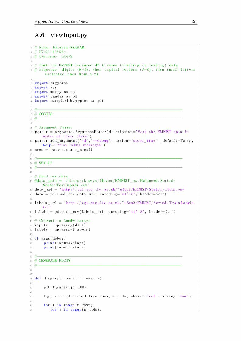
Appendix A. Source Codes 123

A.6 viewInput.py

1 # Name : Eklavya SARKAR,2 # ID :201135564 ,3 # Username : u5es24

5 # Sort the EMNIST Balanced 47 C la s s e s ( t r a i n i n g or t e s t i n g ) data6 # Sequence : d i g i t s (0−9) , then c a p i t a l l e t t e r s (A−Z) , then smal l l e t t e r s

( s e l e c t e d ones from a−z )7

8 import argparse9 import sys

10 import numpy as np11 import pandas as pd12 import matp lo t l i b . pyplot as p l t13

14 #−−−−−−−−−−−−−−−−−−−−−−−−−−−−−−−−−−−−−−−−−−−−−−−−−−−−−−−−−−−−−−−−−15 # CONFIG16 #−−−−−−−−−−−−−−−−−−−−−−−−−−−−−−−−−−−−−−−−−−−−−−−−−−−−−−−−−−−−−−−−−17

18 # Argument Parser19 par s e r = argparse . ArgumentParser ( d e s c r i p t i o n=’ Sort the EMNIST data in

order o f t h e i r c l a s s ’ )20 par s e r . add_argument ( ’−d ’ , ’−−debug ’ , a c t i on=’ store_true ’ , d e f au l t=False ,

he lp=’ Pr int debug messages ’ )21 args = par s e r . parse_args ( )22

23 #−−−−−−−−−−−−−−−−−−−−−−−−−−−−−−−−−−−−−−−−−−−−−−−−−−−−−−−−−−−−−−−−−24 # SET UP25 #−−−−−−−−−−−−−−−−−−−−−−−−−−−−−−−−−−−−−−−−−−−−−−−−−−−−−−−−−−−−−−−−−26

27 # Read raw data28 #data_path = ’/ Users / eklavya /Movies/EMNIST_csv/Balanced/ Sorted /

SortedTest Inputs . csv ’29 data_url = ’ http :// c g i . c s c . l i v . ac . uk/~u5es2 /EMNIST/Sorted /Train . csv ’30 data = pd . read_csv ( data_url , encoding=’ utf−8 ’ , header=None )31

32 l ab e l s_ur l = ’ http :// c g i . c s c . l i v . ac . uk/~u5es2 /EMNIST/Sorted /TrainLabels .txt ’

33 l a b e l s = pd . read_csv ( l abe l s_ur l , encoding=’ utf−8 ’ , header=None )34

35 # Convert to NumPy arrays36 inputs = np . array ( data )37 l a b e l s = np . array ( l a b e l s )38

39 i f a rgs . debug :40 pr in t ( inputs . shape )41 pr in t ( l a b e l s . shape )42

43 #−−−−−−−−−−−−−−−−−−−−−−−−−−−−−−−−−−−−−−−−−−−−−−−−−−−−−−−−−−−−−−−−−44 # GENERATE PLOTS45 #−−−−−−−−−−−−−−−−−−−−−−−−−−−−−−−−−−−−−−−−−−−−−−−−−−−−−−−−−−−−−−−−−46

47

48 de f d i sp l ay ( n_cols , n_rows , x ) :49

50 p l t . f i g u r e ( dpi=100)51

52 f i g , ax = p l t . subp lo t s (n_rows , n_cols , sharex=’ c o l ’ , sharey=’ row ’ )53

54 f o r i in range (n_rows ) :55 f o r j in range ( n_cols ) :

Appendix A. Source Codes 124

56 l a b e l = l a b e l s [ i ]57 p i c = np . rot90 ( ( np . f l i p l r ( inputs [ x , : ] . reshape ( (28 , 28 ) ) ) ) )58 ax [ i , j ] . imshow ( pic , cmap=’ gray ’ )59 ax [ i , j ] . a x i s ( ’ o f f ’ )60 x+=240061 f i g . s a v e f i g ( ’ s t a t i c / images / datase t . png ’ , bbox_inches=’ t i g h t ’ ,

t ransparent=True )62

63 #−−−−−−−−−−−−−−−−−−−−−−−−−−−−−−−−−−−−−−−−−−−−−−−−−−−−−−−−−−−−−−−−−64 # MAIN METHOD CALLS65 #−−−−−−−−−−−−−−−−−−−−−−−−−−−−−−−−−−−−−−−−−−−−−−−−−−−−−−−−−−−−−−−−−66 d i sp l ay (9 , 5 , 0 )

Listing A.6: View input code

125

Appendix B

Data

B.1 Iris Dataset

1 5 . 1 , 3 . 5 , 1 . 4 , 0 . 2 , I r i s −s e t o s a2 4 . 9 , 3 . 0 , 1 . 4 , 0 . 2 , I r i s −s e t o s a3 4 . 7 , 3 . 2 , 1 . 3 , 0 . 2 , I r i s −s e t o s a4 4 . 6 , 3 . 1 , 1 . 5 , 0 . 2 , I r i s −s e t o s a5 5 . 0 , 3 . 6 , 1 . 4 , 0 . 2 , I r i s −s e t o s a6 5 . 4 , 3 . 9 , 1 . 7 , 0 . 4 , I r i s −s e t o s a7 4 . 6 , 3 . 4 , 1 . 4 , 0 . 3 , I r i s −s e t o s a8 5 . 0 , 3 . 4 , 1 . 5 , 0 . 2 , I r i s −s e t o s a9 4 . 4 , 2 . 9 , 1 . 4 , 0 . 2 , I r i s −s e t o s a

10 4 . 9 , 3 . 1 , 1 . 5 , 0 . 1 , I r i s −s e t o s a11 5 . 4 , 3 . 7 , 1 . 5 , 0 . 2 , I r i s −s e t o s a12 4 . 8 , 3 . 4 , 1 . 6 , 0 . 2 , I r i s −s e t o s a13 4 . 8 , 3 . 0 , 1 . 4 , 0 . 1 , I r i s −s e t o s a14 4 . 3 , 3 . 0 , 1 . 1 , 0 . 1 , I r i s −s e t o s a15 5 . 8 , 4 . 0 , 1 . 2 , 0 . 2 , I r i s −s e t o s a16 5 . 7 , 4 . 4 , 1 . 5 , 0 . 4 , I r i s −s e t o s a17 5 . 4 , 3 . 9 , 1 . 3 , 0 . 4 , I r i s −s e t o s a18 5 . 1 , 3 . 5 , 1 . 4 , 0 . 3 , I r i s −s e t o s a19 5 . 7 , 3 . 8 , 1 . 7 , 0 . 3 , I r i s −s e t o s a20 5 . 1 , 3 . 8 , 1 . 5 , 0 . 3 , I r i s −s e t o s a21 5 . 4 , 3 . 4 , 1 . 7 , 0 . 2 , I r i s −s e t o s a22 5 . 1 , 3 . 7 , 1 . 5 , 0 . 4 , I r i s −s e t o s a23 4 . 6 , 3 . 6 , 1 . 0 , 0 . 2 , I r i s −s e t o s a24 5 . 1 , 3 . 3 , 1 . 7 , 0 . 5 , I r i s −s e t o s a25 4 . 8 , 3 . 4 , 1 . 9 , 0 . 2 , I r i s −s e t o s a26 5 . 0 , 3 . 0 , 1 . 6 , 0 . 2 , I r i s −s e t o s a27 5 . 0 , 3 . 4 , 1 . 6 , 0 . 4 , I r i s −s e t o s a28 5 . 2 , 3 . 5 , 1 . 5 , 0 . 2 , I r i s −s e t o s a29 5 . 2 , 3 . 4 , 1 . 4 , 0 . 2 , I r i s −s e t o s a30 4 . 7 , 3 . 2 , 1 . 6 , 0 . 2 , I r i s −s e t o s a31 4 . 8 , 3 . 1 , 1 . 6 , 0 . 2 , I r i s −s e t o s a32 5 . 4 , 3 . 4 , 1 . 5 , 0 . 4 , I r i s −s e t o s a33 5 . 2 , 4 . 1 , 1 . 5 , 0 . 1 , I r i s −s e t o s a34 5 . 5 , 4 . 2 , 1 . 4 , 0 . 2 , I r i s −s e t o s a35 4 . 9 , 3 . 1 , 1 . 5 , 0 . 1 , I r i s −s e t o s a36 5 . 0 , 3 . 2 , 1 . 2 , 0 . 2 , I r i s −s e t o s a37 5 . 5 , 3 . 5 , 1 . 3 , 0 . 2 , I r i s −s e t o s a38 4 . 9 , 3 . 1 , 1 . 5 , 0 . 1 , I r i s −s e t o s a39 4 . 4 , 3 . 0 , 1 . 3 , 0 . 2 , I r i s −s e t o s a40 5 . 1 , 3 . 4 , 1 . 5 , 0 . 2 , I r i s −s e t o s a41 5 . 0 , 3 . 5 , 1 . 3 , 0 . 3 , I r i s −s e t o s a42 4 . 5 , 2 . 3 , 1 . 3 , 0 . 3 , I r i s −s e t o s a43 4 . 4 , 3 . 2 , 1 . 3 , 0 . 2 , I r i s −s e t o s a44 5 . 0 , 3 . 5 , 1 . 6 , 0 . 6 , I r i s −s e t o s a45 5 . 1 , 3 . 8 , 1 . 9 , 0 . 4 , I r i s −s e t o s a46 4 . 8 , 3 . 0 , 1 . 4 , 0 . 3 , I r i s −s e t o s a

Appendix B. Data 126

47 5 . 1 , 3 . 8 , 1 . 6 , 0 . 2 , I r i s −s e t o s a48 4 . 6 , 3 . 2 , 1 . 4 , 0 . 2 , I r i s −s e t o s a49 5 . 3 , 3 . 7 , 1 . 5 , 0 . 2 , I r i s −s e t o s a50 5 . 0 , 3 . 3 , 1 . 4 , 0 . 2 , I r i s −s e t o s a51 7 . 0 , 3 . 2 , 4 . 7 , 1 . 4 , I r i s −v e r s i c o l o r52 6 . 4 , 3 . 2 , 4 . 5 , 1 . 5 , I r i s −v e r s i c o l o r53 6 . 9 , 3 . 1 , 4 . 9 , 1 . 5 , I r i s −v e r s i c o l o r54 5 . 5 , 2 . 3 , 4 . 0 , 1 . 3 , I r i s −v e r s i c o l o r55 6 . 5 , 2 . 8 , 4 . 6 , 1 . 5 , I r i s −v e r s i c o l o r56 5 . 7 , 2 . 8 , 4 . 5 , 1 . 3 , I r i s −v e r s i c o l o r57 6 . 3 , 3 . 3 , 4 . 7 , 1 . 6 , I r i s −v e r s i c o l o r58 4 . 9 , 2 . 4 , 3 . 3 , 1 . 0 , I r i s −v e r s i c o l o r59 6 . 6 , 2 . 9 , 4 . 6 , 1 . 3 , I r i s −v e r s i c o l o r60 5 . 2 , 2 . 7 , 3 . 9 , 1 . 4 , I r i s −v e r s i c o l o r61 5 . 0 , 2 . 0 , 3 . 5 , 1 . 0 , I r i s −v e r s i c o l o r62 5 . 9 , 3 . 0 , 4 . 2 , 1 . 5 , I r i s −v e r s i c o l o r63 6 . 0 , 2 . 2 , 4 . 0 , 1 . 0 , I r i s −v e r s i c o l o r64 6 . 1 , 2 . 9 , 4 . 7 , 1 . 4 , I r i s −v e r s i c o l o r65 5 . 6 , 2 . 9 , 3 . 6 , 1 . 3 , I r i s −v e r s i c o l o r66 6 . 7 , 3 . 1 , 4 . 4 , 1 . 4 , I r i s −v e r s i c o l o r67 5 . 6 , 3 . 0 , 4 . 5 , 1 . 5 , I r i s −v e r s i c o l o r68 5 . 8 , 2 . 7 , 4 . 1 , 1 . 0 , I r i s −v e r s i c o l o r69 6 . 2 , 2 . 2 , 4 . 5 , 1 . 5 , I r i s −v e r s i c o l o r70 5 . 6 , 2 . 5 , 3 . 9 , 1 . 1 , I r i s −v e r s i c o l o r71 5 . 9 , 3 . 2 , 4 . 8 , 1 . 8 , I r i s −v e r s i c o l o r72 6 . 1 , 2 . 8 , 4 . 0 , 1 . 3 , I r i s −v e r s i c o l o r73 6 . 3 , 2 . 5 , 4 . 9 , 1 . 5 , I r i s −v e r s i c o l o r74 6 . 1 , 2 . 8 , 4 . 7 , 1 . 2 , I r i s −v e r s i c o l o r75 6 . 4 , 2 . 9 , 4 . 3 , 1 . 3 , I r i s −v e r s i c o l o r76 6 . 6 , 3 . 0 , 4 . 4 , 1 . 4 , I r i s −v e r s i c o l o r77 6 . 8 , 2 . 8 , 4 . 8 , 1 . 4 , I r i s −v e r s i c o l o r78 6 . 7 , 3 . 0 , 5 . 0 , 1 . 7 , I r i s −v e r s i c o l o r79 6 . 0 , 2 . 9 , 4 . 5 , 1 . 5 , I r i s −v e r s i c o l o r80 5 . 7 , 2 . 6 , 3 . 5 , 1 . 0 , I r i s −v e r s i c o l o r81 5 . 5 , 2 . 4 , 3 . 8 , 1 . 1 , I r i s −v e r s i c o l o r82 5 . 5 , 2 . 4 , 3 . 7 , 1 . 0 , I r i s −v e r s i c o l o r83 5 . 8 , 2 . 7 , 3 . 9 , 1 . 2 , I r i s −v e r s i c o l o r84 6 . 0 , 2 . 7 , 5 . 1 , 1 . 6 , I r i s −v e r s i c o l o r85 5 . 4 , 3 . 0 , 4 . 5 , 1 . 5 , I r i s −v e r s i c o l o r86 6 . 0 , 3 . 4 , 4 . 5 , 1 . 6 , I r i s −v e r s i c o l o r87 6 . 7 , 3 . 1 , 4 . 7 , 1 . 5 , I r i s −v e r s i c o l o r88 6 . 3 , 2 . 3 , 4 . 4 , 1 . 3 , I r i s −v e r s i c o l o r89 5 . 6 , 3 . 0 , 4 . 1 , 1 . 3 , I r i s −v e r s i c o l o r90 5 . 5 , 2 . 5 , 4 . 0 , 1 . 3 , I r i s −v e r s i c o l o r91 5 . 5 , 2 . 6 , 4 . 4 , 1 . 2 , I r i s −v e r s i c o l o r92 6 . 1 , 3 . 0 , 4 . 6 , 1 . 4 , I r i s −v e r s i c o l o r93 5 . 8 , 2 . 6 , 4 . 0 , 1 . 2 , I r i s −v e r s i c o l o r94 5 . 0 , 2 . 3 , 3 . 3 , 1 . 0 , I r i s −v e r s i c o l o r95 5 . 6 , 2 . 7 , 4 . 2 , 1 . 3 , I r i s −v e r s i c o l o r96 5 . 7 , 3 . 0 , 4 . 2 , 1 . 2 , I r i s −v e r s i c o l o r97 5 . 7 , 2 . 9 , 4 . 2 , 1 . 3 , I r i s −v e r s i c o l o r98 6 . 2 , 2 . 9 , 4 . 3 , 1 . 3 , I r i s −v e r s i c o l o r99 5 . 1 , 2 . 5 , 3 . 0 , 1 . 1 , I r i s −v e r s i c o l o r

100 5 . 7 , 2 . 8 , 4 . 1 , 1 . 3 , I r i s −v e r s i c o l o r101 6 . 3 , 3 . 3 , 6 . 0 , 2 . 5 , I r i s −v i r g i n i c a102 5 . 8 , 2 . 7 , 5 . 1 , 1 . 9 , I r i s −v i r g i n i c a103 7 . 1 , 3 . 0 , 5 . 9 , 2 . 1 , I r i s −v i r g i n i c a104 6 . 3 , 2 . 9 , 5 . 6 , 1 . 8 , I r i s −v i r g i n i c a105 6 . 5 , 3 . 0 , 5 . 8 , 2 . 2 , I r i s −v i r g i n i c a106 7 . 6 , 3 . 0 , 6 . 6 , 2 . 1 , I r i s −v i r g i n i c a107 4 . 9 , 2 . 5 , 4 . 5 , 1 . 7 , I r i s −v i r g i n i c a108 7 . 3 , 2 . 9 , 6 . 3 , 1 . 8 , I r i s −v i r g i n i c a109 6 . 7 , 2 . 5 , 5 . 8 , 1 . 8 , I r i s −v i r g i n i c a

Appendix B. Data 127

110 7 . 2 , 3 . 6 , 6 . 1 , 2 . 5 , I r i s −v i r g i n i c a111 6 . 5 , 3 . 2 , 5 . 1 , 2 . 0 , I r i s −v i r g i n i c a112 6 . 4 , 2 . 7 , 5 . 3 , 1 . 9 , I r i s −v i r g i n i c a113 6 . 8 , 3 . 0 , 5 . 5 , 2 . 1 , I r i s −v i r g i n i c a114 5 . 7 , 2 . 5 , 5 . 0 , 2 . 0 , I r i s −v i r g i n i c a115 5 . 8 , 2 . 8 , 5 . 1 , 2 . 4 , I r i s −v i r g i n i c a116 6 . 4 , 3 . 2 , 5 . 3 , 2 . 3 , I r i s −v i r g i n i c a117 6 . 5 , 3 . 0 , 5 . 5 , 1 . 8 , I r i s −v i r g i n i c a118 7 . 7 , 3 . 8 , 6 . 7 , 2 . 2 , I r i s −v i r g i n i c a119 7 . 7 , 2 . 6 , 6 . 9 , 2 . 3 , I r i s −v i r g i n i c a120 6 . 0 , 2 . 2 , 5 . 0 , 1 . 5 , I r i s −v i r g i n i c a121 6 . 9 , 3 . 2 , 5 . 7 , 2 . 3 , I r i s −v i r g i n i c a122 5 . 6 , 2 . 8 , 4 . 9 , 2 . 0 , I r i s −v i r g i n i c a123 7 . 7 , 2 . 8 , 6 . 7 , 2 . 0 , I r i s −v i r g i n i c a124 6 . 3 , 2 . 7 , 4 . 9 , 1 . 8 , I r i s −v i r g i n i c a125 6 . 7 , 3 . 3 , 5 . 7 , 2 . 1 , I r i s −v i r g i n i c a126 7 . 2 , 3 . 2 , 6 . 0 , 1 . 8 , I r i s −v i r g i n i c a127 6 . 2 , 2 . 8 , 4 . 8 , 1 . 8 , I r i s −v i r g i n i c a128 6 . 1 , 3 . 0 , 4 . 9 , 1 . 8 , I r i s −v i r g i n i c a129 6 . 4 , 2 . 8 , 5 . 6 , 2 . 1 , I r i s −v i r g i n i c a130 7 . 2 , 3 . 0 , 5 . 8 , 1 . 6 , I r i s −v i r g i n i c a131 7 . 4 , 2 . 8 , 6 . 1 , 1 . 9 , I r i s −v i r g i n i c a132 7 . 9 , 3 . 8 , 6 . 4 , 2 . 0 , I r i s −v i r g i n i c a133 6 . 4 , 2 . 8 , 5 . 6 , 2 . 2 , I r i s −v i r g i n i c a134 6 . 3 , 2 . 8 , 5 . 1 , 1 . 5 , I r i s −v i r g i n i c a135 6 . 1 , 2 . 6 , 5 . 6 , 1 . 4 , I r i s −v i r g i n i c a136 7 . 7 , 3 . 0 , 6 . 1 , 2 . 3 , I r i s −v i r g i n i c a137 6 . 3 , 3 . 4 , 5 . 6 , 2 . 4 , I r i s −v i r g i n i c a138 6 . 4 , 3 . 1 , 5 . 5 , 1 . 8 , I r i s −v i r g i n i c a139 6 . 0 , 3 . 0 , 4 . 8 , 1 . 8 , I r i s −v i r g i n i c a140 6 . 9 , 3 . 1 , 5 . 4 , 2 . 1 , I r i s −v i r g i n i c a141 6 . 7 , 3 . 1 , 5 . 6 , 2 . 4 , I r i s −v i r g i n i c a142 6 . 9 , 3 . 1 , 5 . 1 , 2 . 3 , I r i s −v i r g i n i c a143 5 . 8 , 2 . 7 , 5 . 1 , 1 . 9 , I r i s −v i r g i n i c a144 6 . 8 , 3 . 2 , 5 . 9 , 2 . 3 , I r i s −v i r g i n i c a145 6 . 7 , 3 . 3 , 5 . 7 , 2 . 5 , I r i s −v i r g i n i c a146 6 . 7 , 3 . 0 , 5 . 2 , 2 . 3 , I r i s −v i r g i n i c a147 6 . 3 , 2 . 5 , 5 . 0 , 1 . 9 , I r i s −v i r g i n i c a148 6 . 5 , 3 . 0 , 5 . 2 , 2 . 0 , I r i s −v i r g i n i c a149 6 . 2 , 3 . 4 , 5 . 4 , 2 . 3 , I r i s −v i r g i n i c a150 5 . 9 , 3 . 0 , 5 . 1 , 1 . 8 , I r i s −v i r g i n i c a

Listing B.1: Iris CSV source code

B.2 Colours Classes

1 0 .976470588 ,0 .921568627 ,0 .9176470592 0 .752941176 ,0 .223529412 ,0 .1686274513 0 .980392157 ,0 .858823529 ,0 .8470588244 0 .690196078 ,0 .227450980 ,0 .1803921575 0 .607843137 ,0 .349019608 ,0 .7137254906 0 .733333333 ,0 .560784314 ,0 .8078431377 0 .831372549 ,0 .901960784 ,0 .9450980398 0 .921568627 ,0 .960784314 ,0 .9843137259 0 .819607843 ,0 .949019608 ,0 .921568627

10 0 .066666667 ,0 .470588235 ,0 .39215686311 0 .086274510 ,0 .627450980 ,0 .52156862712 0 .831372549 ,0 .937254902 ,0 .87450980413 0 .117647059 ,0 .517647059 ,0 .28627451014 0 .094117647 ,0 .415686275 ,0 .23137254915 0 .490196078 ,0 .400000000 ,0 .031372549

Appendix B. Data 128

16 0 .992156863 ,0 .949019608 ,0 .91372549017 0 .901960784 ,0 .494117647 ,0 .13333333318 0 .898039216 ,0 .596078431 ,0 .40000000019 0 .992156863 ,0 .996078431 ,0 .99607843120 0 .592156863 ,0 .603921569 ,0 .60392156921 0 .650980392 ,0 .674509804 ,0 .68627451022 0 .666666667 ,0 .717647059 ,0 .72156862723 0 .800000000 ,0 .819607843 ,0 .81960784324 0 .921568627 ,0 .929411765 ,0 .93725490225 0 .156862745 ,0 .215686275 ,0 .27843137326 0 .670588235 ,0 .698039216 ,0 .72549019627 0 .090196078 ,0 .125490196 ,0 .16470588228 0 .203921569 ,0 .596078431 ,0 .85882352929 0 .160784314 ,0 .501960784 ,0 .72549019630 0 .423529412 ,0 .203921569 ,0 .51372549031 0 .317647059 ,0 .180392157 ,0 .37254902032 0 .921568627 ,0 .870588235 ,0 .94117647133 0 .482352941 ,0 .141176471 ,0 .10980392234 0 .364705882 ,0 .427450980 ,0 .49411764735 0 .439215686 ,0 .482352941 ,0 .48627451036 0 .372549020 ,0 .415686275 ,0 .41568627537 0 .956862745 ,0 .964705882 ,0 .96470588238 0 .898039216 ,0 .905882353 ,0 .91372549039 0 .941176471 ,0 .952941176 ,0 .95686274540 0 .627450980 ,0 .250980392 ,0 .00000000041 0 .470588235 ,0 .258823529 ,0 .07058823542 0 .960784314 ,0 .690196078 ,0 .25490196143 0 .956862745 ,0 .815686275 ,0 .24705882444 0 .670588235 ,0 .921568627 ,0 .77647058845 0 .321568627 ,0 .745098039 ,0 .50196078446 0 .635294118 ,0 .850980392 ,0 .80784313747 0 .203921569 ,0 .596078431 ,0 .858823529

Listing B.2: The colour classes’s source code, employed for theOCR’s mixed digits and letters database

B.3 EMNIST Dataset

Can be accessed on http://cgi.csc.liv.ac.uk/~u5es2/EMNIST/.

129

Appendix C

Art

C.1 Nets

Figure C.1: Incomplete prototype

Appendix C. Art 130

Figure C.2: Complete prototype

Figure C.3: Final design

Appendix C. Art 131

C.2 Volume

Figure C.4: Shadow volume buttons

Figure C.5: Fill volume buttons

Figure C.6: Dash volume buttons

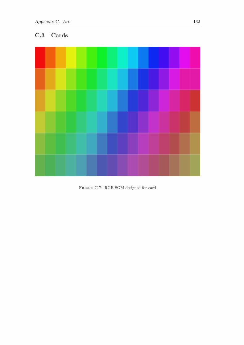
Appendix C. Art 132

C.3 Cards

Figure C.7: RGB SOM designed for card

133

Appendix D

User Manual

D.1 Requirements

To execute the attached scripts, Python 3 is required as a framework.

D.2 Installation

If Python 3 is not already installed, it can be done via brew (which itself can beinstalled with the command given below).

Install Brew:

$/usr/bin/ruby-e"$(curl-fsSLhttps://raw.githubusercontent.com/Homebrew/install/master/install)"

Use Brew to install Python 3:

$python3installpip3

The pip3 package manager is recommended in order to install Flask or any otherPython3 package. To do install, following the steps below, given in a unix shell context.

$pip3installFlask

To run this software, the following libraries are required, and can be installed us-ing pip3:

$pip3installpandas$pip3installnumpy$pip3installmatplotlib

The following used libraries are natively pre-installed in Python, but are nonethelesslisted below:

• argsparse

• sys

• datetime

Appendix D. User Manual 134

Virtual Environments

If necessary, virtual environments can be used to keep the libraries installed for theentire working machine seperate from those simply required for a specific task. Thisensures that the libraries for this project don’t get change or mix up with the devel-opment PC’s native Python installation.

Navigate to ~\myPath\EMNIST-Kohonen-SOM\$pip3installvirtualenv$cdmyPath$virtualenvmyFolder$sourcemyFolder/bin/activate$pip3installmyPackages$deactivate

Running Flask

Finally the proejct can be running by executing app.py on the terminal:

$python3app.py*Runningonhttp://127.0.0.1:5000/(PressCTRL+Ctoquit)

And on a browser simply navigate to: http://127.0.0.1:5000. The website is nowviewable.

135

Appendix E

Use-case descriptions

ID Use Case 1Name Access siteDescription The user accesses the system either via a desktop or mobile

web browserPre-condition System is runningEvent flow 1. Open Browser on device

2. Type in website’s URLID Use Case 2Name Choose Draw ModeDescription The user chooses the draw mode optionPre-condition System is runningEvent flow 1. Click on ‘Draw’ buttonID Use Case 3Name Draw LetterDescription The user draws a letter on the canvasPre-condition System is runningEvent flow 1. Use mouse on desktops, fingers on touchscreen devices

2. Click/touch and drag on canvas to draw3. Draw an alphabet

ID Use Case 4Name Submit DrawingDescription The user submits their input drawing to the backendPre-condition System is runningEvent flow 1. Press the ‘submit’ buttonExtension points Erase DrawingID Use Case 5Name Erase DrawingDescription The user erases all of his current drawingPre-condition System is runningEvent flow 1. Click on ‘Erase’

2. Canvas resets to blank

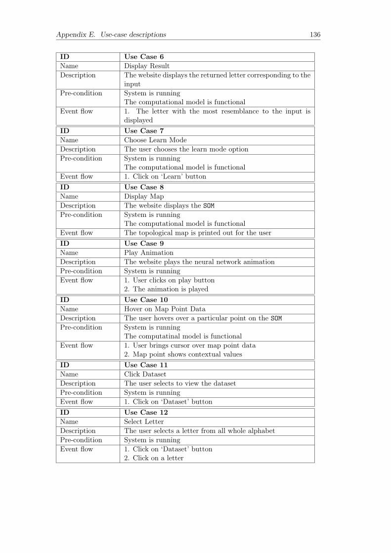
Appendix E. Use-case descriptions 136

ID Use Case 6Name Display ResultDescription The website displays the returned letter corresponding to the

inputPre-condition System is running

The computational model is functionalEvent flow 1. The letter with the most resemblance to the input is

displayedID Use Case 7Name Choose Learn ModeDescription The user chooses the learn mode optionPre-condition System is running

The computational model is functionalEvent flow 1. Click on ‘Learn’ buttonID Use Case 8Name Display MapDescription The website displays the SOMPre-condition System is running

The computational model is functionalEvent flow The topological map is printed out for the userID Use Case 9Name Play AnimationDescription The website plays the neural network animationPre-condition System is runningEvent flow 1. User clicks on play button

2. The animation is playedID Use Case 10Name Hover on Map Point DataDescription The user hovers over a particular point on the SOMPre-condition System is running

The computatinal model is functionalEvent flow 1. User brings cursor over map point data

2. Map point shows contextual valuesID Use Case 11Name Click DatasetDescription The user selects to view the datasetPre-condition System is runningEvent flow 1. Click on ‘Dataset’ buttonID Use Case 12Name Select LetterDescription The user selects a letter from all whole alphabetPre-condition System is runningEvent flow 1. Click on ‘Dataset’ button

2. Click on a letter

Appendix E. Use-case descriptions 137

ID Use Case 13Name Select CharacterDescription The user selects a given character of the chosen letterPre-condition System is runningEvent flow 1. Click on ‘Dataset’ button

2. Click on a letter3. Click on a specific letter4. Click

ID Use Case 14Name Display CharactersDescription The website displays the meta data on the chosen characterPre-condition System is runningEvent flow The meta-data on such a character is displayed as a pop-upID Use Case 15Name Close SiteDescription The user shuts down the browserPre-condition System is runningEvent flowExtension pointsTriggersPost-condition The user exists the browser

138

Appendix F

Testing

F.1 Hardware

The testing of the application was done on the following hardware device:

Macbook Pro 15" Retina (1st Gen), early 20131:

• OS: macOS High-Sierra

• Processor: 2.4 GHz Intel Core i7

• Memory: 8 GB 1600 MHz DDR3

• Graphics: NVIDIA GeForce GT 650M 1024 MB, Intel HD Graphics 4000 1536MB

F.2 Software

Google Chrome’s browser in developer mode also allows testing in various screen sizesand resolutions which was thoroughly used for UI formatting testing. This allowedto maintain a universal look and feel of the website across different devices, and isn’texclusively device-dependent.

The developer PC’s task manager also allowed to monitor for any eventual mem-ory leaks or excessive CPU usages, and was be used to optimise the web application.This was of relative importance as battery life is generally important, and a bad expe-rience could deter people from using the website again. Network usage of website wasalso be looked at to decide whether or not to optimise or compress certain features.

F.3 Test Results

The following is the testing results of the different scripts. Each test ID was executedwith the command $Python3ScriptName.py following by any extra CLI parameter,such as -d. The parameters for each test case is given in the table, and a blank valuerepresents no additional argument being parsed.

1MacBook Pro (Retina, 15-inch, Early 2013) - Technical Specifications. https://support.apple.com/kb/sp669?locale=en_US. (Accessed on 05/05/2018).

Appendix F. Testing 139

F.3.1 RGB

ID Data Data Type Expected Result Success?1 (Blank) Correct Successful build YES2 -i Erroneous Native error message YES3 -i= Erroneous Native error message YES4 -i=0 Erroneous Implemented error message YES5 -i=-1 Erroneous Implemented error message YES6 -i=0.5 Erroneous Native error message YES7 -i=-0.5 Erroneous Native error message YES8 -i=100 Correct Successful build YES9 -r Erroneous Native error message YES10 -r= Erroneous Native error message YES11 -r=0 Erroneous Implemented error message YES12 -r=-1 Erroneous Implemented error message YES13 -r=0.5 Correct Successful build YES14 -r=1 Correct Successful build YES15 -r=1.5 Erroneous Implemented error message YES16 -d Correct Successful build YES17 -d-i=100 Correct Successful build YES18 -d-r=0.3 Correct Successful build YES19 -r=0.3-i=100 Correct Successful build YES20 -d-r=0.3-i=100 Correct Successful build YES

Table F.1: RGB script tests

F.3.2 Iris

ID Data Type Expected Result Success?1 (Blank) Correct Successful build YES2 -r Erroneous Native error message YES3 -r= Erroneous Native error message YES4 -r=0 Erroneous Implemented error message YES5 -r=-1 Erroneous Implemented error message YES6 -r=0.5 Correct Successful build YES7 -r=1 Correct Successful build YES8 -r=1.5 Erroneous Implemented error message YES9 -d Correct Successful build YES10 -d-r=0.3 Correct Successful build YES

Table F.2: Iris script tests

Appendix F. Testing 140

F.3.3 OCR

ID Data Type Expected Result Success?1 (Blank) Correct Successful build YES2 -d Correct Successful build YES3 -r Erroneous Native error message YES4 -r= Erroneous Native error message YES5 -r=0 Erroneous Implemented error message YES6 -r=-1 Erroneous Implemented error message YES7 -r=0.5 Correct Successful build YES8 -r=1 Correct Successful build YES9 -r=1.5 Erroneous Implemented error message YES10 -iTr=100 Correct Successful build YES11 -iTr=0 Correct Successful build YES12 -iTr=-1 Erroneous Implemented error message YES13 -iTr=2400 Correct Successful build YES14 -iTr=2401 Erroneous Implemented error message YES15 -iTe=100 Correct Successful build YES16 -iTe=0 Correct Successful build YES17 -iTe=-1 Erroneous Implemented error message YES18 -iTe=2400 Correct Successful build YES19 -iTe=2401 Erroneous Implemented error message YES20 -t=d Correct Successful build YES21 -t=l Correct Successful build YES22 -t=c Correct Successful build YES23 -t=z Erroneous Implemented error message YES24 -d-iTr=100 Correct Successful build YES25 -d-iTe=100 Correct Successful build YES26 -d-r=0.3 Correct Successful build YES27 -d-r=0.3-iTr=100 Correct Successful build YES28 -d-r=0.3-iTr=100-iTe=100 Correct Successful build YES29 -d-r=0.3-iTr=100-iTe=100-t=d Correct Successful build YES

Table F.3: OCR script tests

141

Appendix G

Web-Pages

Figure G.1: Page 1

Appendix G. Web-Pages 142

Figure G.2: Page 2

Figure G.3: Page 3

Appendix G. Web-Pages 143

Figure G.4: Page 4

Figure G.5: Page 5

Appendix G. Web-Pages 144

Figure G.6: Page 6

Figure G.7: Page 7

Appendix G. Web-Pages 145

Figure G.8: Page 8

Figure G.9: Page 9

Appendix G. Web-Pages 146

Figure G.10: Page 10

Figure G.11: Page 11

Appendix G. Web-Pages 147

Figure G.12: Page 12

Figure G.13: Page 13

Appendix G. Web-Pages 148

Figure G.14: Page 14

Figure G.15: Page 15

Appendix G. Web-Pages 149

Figure G.16: Page 16

Figure G.17: Page 17

Appendix G. Web-Pages 150

Figure G.18: Page 18

151

Appendix H

Plots

H.1 RGB

H.1.1 0.3 Learning Rate, 1000 Inputs

Figure H.1: RGB Plot 1

Appendix H. Plots 152

Figure H.2: RGB Plot 2

Figure H.3: RGB Plot 3

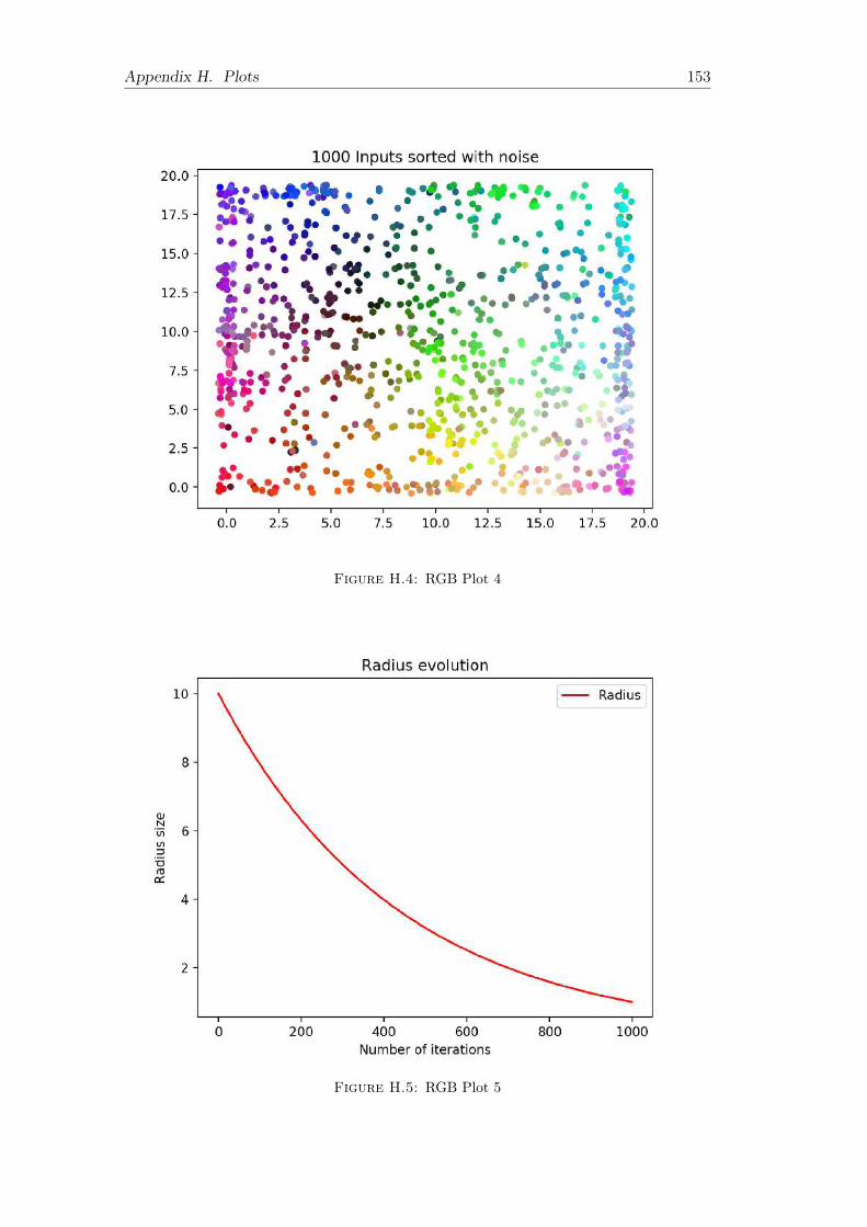
Appendix H. Plots 153

Figure H.4: RGB Plot 4

Figure H.5: RGB Plot 5

Appendix H. Plots 154

Figure H.6: RGB Plot 6

Appendix H. Plots 155

H.2 Iris

H.2.1 0.3 Learning Rate

Figure H.7: Iris Plot 1

Appendix H. Plots 156

Figure H.8: Iris Plot 2

Figure H.9: Iris Plot 3

Appendix H. Plots 157

Figure H.10: Iris Plot 4

Figure H.11: Iris Plot 5

Appendix H. Plots 158

Figure H.12: Iris Plot 6

Figure H.13: Iris Plot 7

Appendix H. Plots 159

H.2.2 0.8 Learning Rate

Figure H.14: Iris Plot 8

Appendix H. Plots 160

Figure H.15: Iris Plot 9

Figure H.16: Iris Plot 10

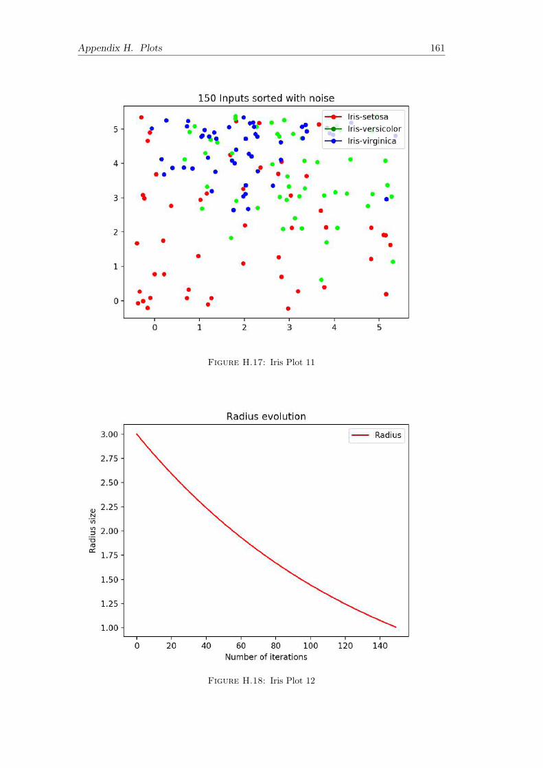
Appendix H. Plots 161

Figure H.17: Iris Plot 11

Figure H.18: Iris Plot 12

Appendix H. Plots 162

Figure H.19: Iris Plot 13

Figure H.20: Iris Plot 14

Appendix H. Plots 163

H.3 OCR

H.3.1 0.3 Learning Rate, 100 Training Inputs, 10 Testing Inputs

Figure H.21: OCR Plot 1

Appendix H. Plots 164

Figure H.22: OCR Plot 2

Figure H.23: OCR Plot 3

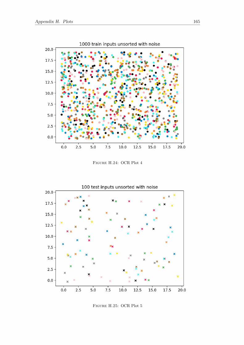
Appendix H. Plots 165

Figure H.24: OCR Plot 4

Figure H.25: OCR Plot 5

Appendix H. Plots 166

Figure H.26: OCR Plot 6

Figure H.27: OCR Plot 7

Appendix H. Plots 167

Figure H.28: OCR Plot 8

Figure H.29: OCR Plot 9

Appendix H. Plots 168

Figure H.30: OCR Plot 10

Figure H.31: OCR Plot 11

Appendix H. Plots 169

Figure H.32: OCR Plot 12

Figure H.33: OCR Plot 13

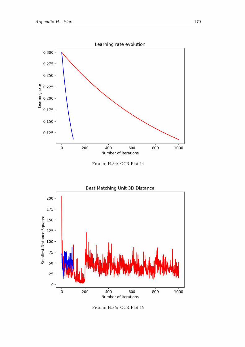
Appendix H. Plots 170

Figure H.34: OCR Plot 14

Figure H.35: OCR Plot 15

171

Bibliography

[1] Artificial neural network - wikipedia. https://en.wikipedia.org/wiki/Artificial_neural_network. (Accessed on 11/16/2017).

[2] Bootstrap. https://getbootstrap.com/. (Accessed on 04/02/2018).

[3] Cluster analysis - wikipedia. https://en.wikipedia.org/wiki/Cluster_analysis. (Accessed on 11/16/2017).

[4] The emnist dataset | nist. https://www.nist.gov/itl/iad/image-group/emnist-dataset. (Accessed on 11/16/2017).

[5] Emnist (extended mnist) | kaggle. https://www.kaggle.com/crawford/emnist.(Accessed on 04/25/2018).

[6] Machine learning | coursera. https://www.coursera.org/learn/machine-learning/. (Accessed on 11/16/2017).

[7] Matplotlib 2.2.2 documentation. https://matplotlib.org/. (Accessed on04/02/2018).

[8] The neural network zoo - the asimov institute. http://www.asimovinstitute.org/neural-network-zoo/. (Accessed on 04/26/2018).

[9] Numpy and scipy documentation. https://docs.scipy.org/doc/. (Accessedon 04/02/2018).

[10] Pattern recognition - wikipedia. https://en.wikipedia.org/wiki/Pattern_recognition. (Accessed on 04/25/2018).

[11] Pattern recognition (psychology) - wikipedia. https://en.wikipedia.org/wiki/Pattern_recognition_(psychology). (Accessed on 04/25/2018).

[12] Self-organizing map - wikipedia. https://en.wikipedia.org/wiki/Self-organizing_map. (Accessed on 11/16/2017).

[13] Som tutorial. http://www.ai-junkie.com/ann/som/som1.html. (Accessed on11/16/2017).

[14] Asboth, D. Self-organising maps: An introduction. http://davidasboth.com/2016/11/05/self-organising-maps-an-introduction/. (Accessed on04/02/2018).

[15] Cohen, G., Afshar, S., Tapson, J., and Van Schaik, A. EMNIST: anextension of MNIST to handwritten letters. CoRR abs/1702.05373 (2017).

[16] Dheeru, D., and Karra Taniskidou, E. UCI machine learning repository,2017.

BIBLIOGRAPHY 172

[17] Eichner, H. Neural net for handwritten digit recognition in javascript. http://myselph.de/neuralNet.html. (Accessed on 11/16/2017).

[18] Fiesler, E., and Beale, R., Eds. Handbook of Neural Computation. OxfordUniversity Press, 1997.

[19] H. Ott, B. A convergence criterion for self-organising maps. Master’s thesis,University of Rhode Island, 2012.

[20] Jongejan, J., Rowley, H., Kawashima, T., Kim, J., and Fox-Gieg, N.Quick, draw! https://quickdraw.withgoogle.com/. (Accessed on 11/16/2017).

[21] Kohonen, T. Self-Organizing Maps, 3rd ed. Springer-Verlag New York, Inc.,Secaucus, NJ, USA, 2001.

[22] Kohonen, T. Essentials of the self-organizing map. Neural Networks 37 (2013),52 – 65. Twenty-fifth Anniversay Commemorative Issue.

[23] LeCun, Y., Cortes, C., and Burges, C. Mnist handwritten digit database.http://yann.lecun.com/exdb/mnist/. (Accessed on 11/16/2017).

[24] Murphy, K. P. Machine Learning: A Probabilistic Perspective. The MIT Press,2012.

[25] Olah, C. Visualizing mnist: An exploration of dimensionality reduction.http://colah.github.io/posts/2014-10-Visualizing-MNIST. (Accessed on11/16/2017).

[26] Ronacher, A. Flask (a python microframework). http://flask.pocoo.org/.(Accessed on 11/16/2017).

[27] Russell, S. J., and Norvig, P. Artificial Intelligence: A Modern Approach,2 ed. Pearson Education, 2003.

[28] TensorFlow. Mnist for ml beginners. https://www.tensorflow.org/get_started/mnist/beginners. (Accessed on 10/15/2017).

[29] Wang, Y. Artificial neural networks: Kohonen self-organizing maps (soms).Bachelor thesis, University of Liverpool, May 2015.

[30] Westerlund, M. L. Classification with kohonen self-organising maps. SoftComputing, Haskoli Islands (2005).

[31] Zurada, J. M. Introduction to Artificial Neural Systems. West Publishing Co.,St. Paul, MN, USA, 1992.