arX

iv:h

ep-t

h/98

1025

0v1

30

Oct

199

8

3-Sasakian Manifolds

Charles P. Boyer and Krzysztof Galicki

An Introduction

We begin this review with a brief history of the subject for our exposition shallhave little to do with the chronology. In 1960 Sasaki [Sas 1] introduced a geometricstructure related to an almost contact structure. This geometry became known as Sasakiangeometry and has been studied extensively ever since. In 1970 Kuo [Kuo] refined thisnotion and introduced manifolds with Sasakian 3-structures (see also [Kuo-Tach, Tach-Yu]). Independently, the same concept was invented by Udriste [Ud]. Between 1970and 1975 this new kind of geometry was investigated almost exclusively by a group ofJapanese geometers, including Ishihara, Kashiwada, Konishi, Kuo, Tachibana, Tanno,and Yu. Already in [Kuo] we learn that the 3-Sasakian geometry has some interestingtopological implications. Using earlier results of Tachibana about the harmonic forms oncompact Sasakian spaces [Tach], Kuo showed that odd Betti numbers up to the middledimension must be divisible by 4. In 1971 Kashiwada observed that every 3-Sasakianmanifold is Einstein with a positive Einstein constant [Kas]. In the same year Tanno provedan interesting theorem about the structure of the isometry group of every 3-Sasakian space[Tan 1]. In a related paper he studied a natural 3-dimensional foliation on such spacesshowing that, if the foliation is regular, then the space of leaves is an Einstein manifold ofpositive scalar curvature [Tan 2]. Tanno clearly points to the importance of the analogywith the quaternionic Hopf fibration S3 → S7 → S4, but does not go any further. In fact,Kashiwada’s paper mentions a conjecture speculating that every 3-Sasakian manifold is ofconstant curvature [Kas]. She attributed this conjecture to Tanno and, at the time, thesewere the only known examples.

Very soon after, however, it became clear that such a conjecture could not possibly betrue. This is due to a couple of papers by Ishihara and Konishi [I-Kon, Ish 1]. They madea fundamental observation that the space of leaves of the natural 3-dimensional foliationsmentioned above has a “quaternionic structure”, part of which is the Einstein metricdiscovered by Tanno. This led Ishihara to an independent study of this “sister geometry”:quaternionic Kahler manifolds [Ish 2]. His paper is very well-known and is almost alwayscited as the source of the explicit coordinate description of quaternionic Kahler geometry.Among other results Ishihara showed that his definition implies that the holonomy groupof the metric is a subgroup of Sp(n)·Sp(1), thus providing an important connection withthe earlier studies of such manifolds by Alekseevsky [Al 1], Bonan [Bon], Gray [Gra 1],Kraines [Kra], and Wolf [Wol]. In 1975 Konishi [Kon] proved the existence of a Sasakian3-structure on a natural principal SO(3)-bundle over any quaternionic Kahler manifoldof positive scalar curvature. This, with the symmetric examples of Wolf, gives preciselyall of the homogeneous 3-Sasakian spaces. Yet, at the time they did not appear explicitlyand escaped any systematic study until much later.

In fact, 1975 seems to be the year when 3-Sasakian manifolds are relegated to analmost complete obscurity which lasted for about 15 years. From that point on the two“sisters” fair very differently. The extent of this can be best illustrated by the famousbook on Einstein manifolds by Besse [Bes]. The book appeared in 1987 and provided thereader with an excellent, up-to-date, and very complete account of what was known about

During the preparation of this work the authors were supported by an NSF grant.

1

Einstein manifolds 10 years ago. But one is left in the dark when trying to find referencesto any of the papers on 3-Sasakian manifolds we have cited; 3-Sasakian manifolds arenever mentioned in Besse. The other “sister”, on the contrary, received a lot of spacein a separate chapter. Actually Einstein metrics on Konishi’s bundle do appear in Besse(see [Bes] 14.85, 14.86) precisely in the context of the SO(3)-bundles over positive quater-nionic Kahler manifolds as a consequence of a theorem of Berard-Bergery ([Bes], 9.73).Obviously, the absence of 3-Sasakian spaces in Besse’s book was the result rather than thecause of this obscurity. One could even say it was justified by the lack of any interestingexamples. The authors have puzzled over this phenomenon without any sound explana-tion. One can only speculate that it is the holonomy reduction that made quaternionicKahler manifolds so much more attractive an object. Significantly, the holonomy groupof a 3-Sasakian manifold never reduces to a proper subgroup of the special orthogonalgroup. And when in 1981 Salamon [Sal 1,2], independently with Berard-Bergery [BeBer],generalized Penrose’s twistor construction for self-dual 4-manifolds introducing the twistorspace over an arbitrary quaternionic Kahler manifold, the research on quaternionic Kahlergeometry flourished, fueled by powerful tools from complex algebraic geometry.

Finally, in the early nineties, 3-Sasakian manifolds start a comeback. They begin toappear in two completely different contexts. First, in the study of manifolds with realKilling spinors, Friedrich and Kath notice that the existence of one such spinor leadsnaturally to a Sasakian-Einstein structure while three of them give the manifold a 3-Sasakian structure [B-G-F-K, Fr-Kat 1]. Assuming regularity they are able to combinethe result of Hitchin [Hit 1] and Friedrich and Kurke [Fr-Kur] and obtain a classificationof all regular complete 7-manifolds with 3-Sasakian structure [Fr-Kat 2]. This appearsto be the first classification result about 3-Sasakian manifolds. In 1993 the classificationproblem for manifolds admitting Killing spinors found an elegant formulation in terms ofholonomy groups [Bar]. Bar observes that if (M, g) is a simply connected spin manifoldwith a non-trivial real Killing spinor then the metric cone (C(M), g) must admit a parallelspinor. In particular (C(M), g) is Ricci-flat and Hol(g) is quite restricted so that only veryfew groups can occur. One such possibility is Hol(g) = Sp(m+ 1) which gives the cone ahyperkahler structure. It easily follows that M must be 3-Sasakian.

Independently, the hyperkahler geometry of the cone C(S) was the starting pointof our research on 3-Sasakian manifold. In 1991 the authors, together with Ben Mann,discovered that 3-Sasakian manifolds appear naturally as levels sets of a certain momentmap on a hyperkahler manifold with an isometric SU(2)-action rotating the triple ofcomplex structures [B-G-M 1]. In fact, if some obstructions for the SU(2)-action vanish,then the hyperkahler manifold is precisely a cone on a 3-Sasakian space and, at the sametime, it is the Swann’s bundle over the associated quaternionic Kahler orbifold of positivescalar curvature [Sw]. We quickly realized that S is ultimately related to three otherEinstein geometries: its hyperkahler cone C(S), the associated twistor space Z, and theassociated quaternionic Kahler orbifold O. In this review we call the collection of thesefour geometries together with all the relevant maps ♦(S). Thus, every S comes togetherwith a fundamental diagram

C(S)ւ ց

Z ←−−−−−−−

y

S.ց ւ

O

More importantly we also realized that, even when O and Z are compact Riemannian

2

orbifolds, S can be a smooth manifold. This moment marks the beginning of our effortsto understand the geometry and topology of 3-Sasakian manifolds.

They have led us through the classification of all 3-Sasakian homogeneous spaces and adiscovery of a new quotient construction of infinitely many homotopy types of non-regularcompact 3-Sasakian manifolds [B-G-M-2]. In dimension 7 these examples turned out tobe certain Eschenburg bi-quotients of U(3) by a 2-torus [Esch 1-2]. We gave a completeanalysis of the geometry and topology of such spaces [B-G-M 2]. The next important stepwas the second author’s work with Simon Salamon [G-Sal]. There we noticed that Kuo’stheorem about odd Betti numbers of 3-Sasakian manifolds being divisible by 4 missed acrucial point. Because of the isometric SU(2)-action, all odd Betti numbers up to themiddle dimension must actually vanish. In the regular case we were able to show that 3-Sasakian cohomology is just the primitive cohomology of both Z andO. These results werethen extended to the orbifold case in [B-G 1], where we also made a systematic study of theorbifold twistor spaces Z and gave an orbifold extension of the LeBrun’s inversion theorem[Le 3]. Finally, the Vanishing Theorem for Betti numbers provided us with the tools tostudy the geometry and topology of more complicated examples. This study [B-G-M-R1,2] used a rational spectral sequence and culminated in discovering that, in dimension7, all rational homology types not excluded by the Vanishing Theorem do occur and canbe constructed explicitly. These examples illustrate the richness of 3-Sasakian geometryin dimension 7. For example, there is an infinite family of 3-Sasakian 7-manifolds thatadmit metrics of positive sectional curvature, while there is another infinite family thatcan admit no metrics whose sectional curvature is bounded below by an arbitrary fixednegative number! Later in [B-G-M 8] we discovered how to handle the integral spectralsequence giving integral results for our 7-dimensional examples up through the secondhomology group. We also studied [B-G-M 7] the higher dimensional analogue showingthat these meet with an entirely different fate.

This review chapter is intended to give the reader a self-contained account of every-thing we have learned about such spaces to date. We have tried to gather all the knownresults. In a chapter like this it would be impossible to present every proof so we do quotesome theorems just referring to the literature. But we have tried to include as many proofsas possible so that the review is not simply a long dry list of theorems, propositions, andcorollaries. When it comes to references we make no claim of completeness, though wehave tried to do our best. We apologize for any omissions. At the end we hope to be ableto convince our reader that the 3-Sasakian geometry is at least as fascinating as any other“sister” geometry of the fundamental diagram ♦(S).

Our review is organized as follows: We begin by setting up definitions, notation, anddescribing elementary properties of Sasakian, Sasakian-Einstein, and 3-Sasakian manifoldsin Section 1. Next we discuss fundamentals about the geometry of the associated foliations(arrows in the diagram ♦(S)). We then give a classification of homogeneous geometriesin Section 3. Section 4 is all about Betti numbers of Sasakian and 3-Sasakian manifoldswhile Section 5 is a very brief look at the Killing spinors and G2 structures. The followingsection describes the geometry of the 3-Sasakian quotient construction. After this wegive a detailed study of “toric” 3-Sasakian manifolds. We conclude with a handful ofopen problems, questions, and some conjectures followed by an appendix on fundamentalproperties of orbifolds.

Acknowledgments: The authors would like thank Ben Mann who is a friend and hasbeen a collaborator on much of our work. We also thank our other collaborators SimonSalamon and Elmer Rees. We thank Roger Bielawski, Alex Buium, Claude LeBrun, LiviuOrnea, and Uwe Semmelmann for discussions and valuable comments. Last, but not least,the second named author would like to than Max-Planck-Institute fur Mathematik in Bonnfor support and hospitality. This review was written during his stay in Bonn.

3

1. Definitions and Basic Properties

In this section we introduce notation, definitions, and discuss some elementary prop-erties of Sasakian, Sasakian-Einstein, and 3-Sasakian manifolds. Traditionally Sasakianstructures were defined via contact structures by adding a Riemannian metric with someadditional conditions. We take a simpler and more geometric approach that uses theholonomy reduction of the associated metric cone.

1.1 Sasakian Manifolds

Definition 1.1.1: Let (S, g) be a Riemannian manifold of real dimension m. We say that(S, g) is Sasakian if the holonomy group of the metric cone on S(C(S), g) = (R+ × S, dr2 + r2g) reduces to a subgroup of U(m+1

2). In particular,

m = 2n+ 1, n ≥ 1 and (C(S), g) is Kahler.

The following proposition provides three alternative characterizations of the Sasakianproperty, the first one, perhaps, most in the spirit of the the original definition of Sasaki[Sas 1]:

Proposition 1.1.2: Let (S, g) be a Riemannian manifold, ∇ the Levi-Civita connectionof g, and let R(X, Y ) : Γ(TS)→ Γ(TS) denote the Riemann curvature tensor of ∇. Thenthe following conditions are equivalent:

(i) There exists a Killing vector field ξ of unit length on S so that the tensor field Φ oftype (1, 1), defined by Φ(X) = ∇Xξ, satisfies the condition

1.1.3 (∇XΦ)(Y ) = g(ξ, Y )X − g(X, Y )ξ

for any pair of vector fields X and Y on S.(ii) There exists a Killing vector field ξ of unit length on S so that the Riemann curvature

satisfies the condition

1.1.4 R(X, ξ)Y = g(ξ, Y )X − g(X, Y )ξ,

for any pair of vector fields X and Y on S.(iii) There exists a Killing vector field ξ of unit length on S so that the sectional curvature

of every section containing ξ equals one.

(iv) (S, g) is Sasakian.

Proof: We outline the proof of the equivalence of (i) and (iv). The equivalence of (i) and(ii) is a simple calculation relating (∇XΦ)(Y ) to R(X, ξ)Y and is left to the reader (see[Y-K]). The equivalence of (ii) and (iii) is obvious.

We first show how (iv) implies (i). Let X, Y be any two vector fields on S viewedas vector fields on C(S) and ∇ be the Levi-Civita connection of g. Then we have thefollowing warped product formulas for the cone metric connection [O’N, p. 206]:

1.1.5 ∇∂r∂r = 0, ∇∂r

X = ∇X∂r =1

rX, ∇XY = ∇XY − rg(X, Y )∂r.

Since the holonomy group of the cone (C(S), g) reduces to a subgroup of U(m+12 )

there is a parallel complex structure I on C(S), i.e., I commutes with ∇. We can identifyS with S × 1 ⊂ C(S) and define

1.1.6 ξ = I(∂r), η(Y ) = g(ξ, Y ), Φ(Y ) = ∇Y ξ

4

for any vector field Y ∈ Γ(TS). It is then a simple calculation to show that ξ is actuallya unit Killing vector field on S and it satisfies the curvature condition 1.1.3. Clearly, ξ isunit by definition and we have

g(∇Y ξ,X) = g(∇Y ξ + g(ξ, Y )∂r, X) = g(∇Y I(∂r), X) =

= g(I(∇Y ∂r), X) = g(I(Y ), X)

which is skew-symmetric inX and Y . The second condition follows from ∇I = 0, definitionof Φ(Y ) = ∇Y (I∂r), and the formulas 1.1.5. Conversely, we can construct a Kahlerstructure on C(S) as follows: Let Ψ = r∂r denote the Euler field on C(S) and definesmooth section of End TC(S) by the formula

1.1.7 IY = Φ(Y )− η(Y )Ψ, IΨ = ξ,

where η(Y ) = g(ξ, Y ) is the dual 1-form of ξ. It is easy to see that I is an almost complexstructure on C(S) and the metric g is Hermitian. To show that C(S) is Kahler it is enoughto show that ∇I = 0. This is done by a direct calculation using the definition of I andequations 1.1.6.

The above discussion shows that there is a natural splitting of the tangent bundleTC(S) as TC(S) = LΨ ⊕ Lξ ⊕H where LX denotes the trivial line bundle generated bythe nowhere vanishing vector field X, and H is a complement with respect to the metricg. It follows immediately that the frame bundle of any Sasakian manifold of dimension2n+ 1 reduces to the group 1× U(n) [Sas 1]. It follows that every Sasakian manifold hasa canonical Spinc structure [Mor].

In view of the above proposition the triple ξ, η,Φ is called a Sasakian structureon (S, g), the Killing vector field ξ and the 1-form η are called the characteristic vectorfield and the characteristic 1-form of the Sasakian structure, respectively. We next givesome elementary properties of Sasakian structures. All of them follow as an immediateconsequence of the definition and Proposition 1.1.2.

Proposition 1.1.8: Let (S, g) be a Sasakian manifold, ξ, η,Φ its Sasakian structure,and X and Y any pair of vector fields on S. Furthermore, let NΦ(Y,X) = [ΦY,ΦX ] +Φ2[Y,X ]− Φ[Y,ΦX ]− Φ[ΦY,X ] be the Nijenhuis torsion tensor of Φ. Then

(i) ΦΦ(Y ) = −Y + η(Y )ξ,

(ii) Φξ = 0, η(ΦY ) = 0,

(iii) g(X,ΦY ) + g(ΦX, Y ) = 0, g(ΦY,ΦX) = g(Y,X)− η(Y )η(X),

(iv) dη(Y,X) = 2g(ΦY,X), NΦ(Y,X) = dη(Y,X)⊗ ξ.

A Sasakian manifold is not necessarily Einstein. As a simple consequence of therelation between Ricci curvature of S and its metric cone C(S), the Einstein conditioncan be expressed in terms of Ricci-flatness of the cone metric g and we get

5

Proposition 1.1.9: Let (S, g) be be a Sasakian manifold of dimension 2n + 1. Thenthe metric g is Einstein if and only if the cone metric g is Ricci-flat, i.e., (C(S), g) isKahler Ricci-flat (Calabi-Yau). In particular, it follows that the restricted holonomy group

Hol0(g) ⊂ SU(n+ 1) and that the Einstein constant of g is positive and equals 2n.

An immediate consequence of the this proposition and Myers’ Theorem is:

Corollary 1.1.10: A complete Sasakian-Einstein manifold is compact with diameterless than or equal to π and with finite fundamental group.

Now Hol0(g) is the normal subgroup of the full holonomy group Hol(g) that is thecomponent connected to the identity. There is a canonical epimorphism

π1(S) = π1(C(S))−−→Hol(g)/Hol0(g),

so if S is simply-connected its structure group reduces to 1 × SU(n) and it will admit aspin structure. We have

Corollary 1.1.11: Let S be a Sasakian-Einstein manifold such that the full holonomygroup of the cone metric Hol(g) is contained in SU(m+1). Then S admits a spin structure.In particular, every simply-connected Sasakian-Einstein manifold admits a spin structure.

We give some examples that illustrate the complications in the presence of funda-mental group. The hypothesis of this corollary is not necessary as the second exampleshows.Examples 1.1.12: The real projective space S = RP2n+1 with its canonical metric isSasakian-Einstein, and the cone C(S) = (Cn+1 − 0)/Z2 with the usual antipodal iden-tification. We have Hol(g) ≃ π1(S) ≃ Z2. When n is odd the antipodal map τ is inSU(n+1), so S = RP2n+1 admits a spin structure. But when n is even the antipodal mapτ does not lie in SU(n + 1), which obstructs a further reduction of the structure group.In this case it is well-known that S = RP2n+1 does not admit a spin structure. In fact thegenerator of Hol(g) ≃ Z2 is the obstruction. There are many other similar examples. Anexample that shows that the hypothesis in Corollary 1.1.11 is not necessary is the following:Consider the lens space L(p; , q1, · · · , qn) ≃ S2n+1/Zp where the qi’s are relatively primeto p. The action on Cn+1 − 0 is generated by (z0, z1, · · · , zn) 7→ (ηz0, η

q1z1, · · · , ηqnzn)where η is a primitive pth root of unity. It is known [Fra] that if p is odd, L(p; q1, · · · , qn)admits a spin structure. However, if

∑

i qi + 1 is not divisible by p, the holonomy groupHol(g) ≃ Zp does not lie in SU(n+ 1).

Let S be a Sasakian manifold, suppose that the characteristic vector field ξ is complete.Since ξ has unit norm, it defines a 1-dimensional foliation F on S. We shall be interestedin the case when all the leaves of F are compact.

Definition 1.1.13: Let (S, g) be be a compact Sasakian manifold and let F be the 1-dimensional foliation defined by ξ. We say that S is quasi-regular if the foliation F isquasi-regular, i.e., each point p ∈ S has a cubical neighborhood U such that any leaf L ofF intersects a transversal through p at most a finite number of times N(p). Furthermore,S is called regular if N(p) = 1 for all p ∈ S.

It is known that the quasi-regular property is equivalent to the condition that all theleaves of the foliation are compact. In the regular case, the foliation F is simple, anddefines a global submersion. In fact it defines a principal S1 bundle over its space ofleaves. In the quasi-regular case it is well-known [Tho, Mol] that ξ generates a locally freecircle action on S, and that the space of leaves is a compact orbifold (See the appendixfor a brief review of orbifolds and their relation to foliations, in particular see A.3). We

6

shall denote the space of leaves of the foliation F on S by Z. Then the natural projectionπ : S−−→Z is a Siefert fibration. It is an example of what we call a principal V-bundleover Z. In Section 2 we shall study this foliation in detail.

1.2 3-Sasakian Spaces

Using all the definitions of the previous section we now describe a more specializedsituation. Again, this can be done by an additional holonomy reduction requirement.

Definition 1.2.1: Let (S, g) be a Riemannian manifold of real dimension m. We say that(S, g) is 3-Sasakian if the holonomy group of the metric cone on S(C(S), g) = (R+ × S, dr2 + r2g) reduces to a subgroup of Sp(m+1

4 ). In particular,m = 4n+ 3, n ≥ 1 and (C(S), g) is hyperkahler.

Since C(S) is hyperkahler it has a hypercomplex structure I1, I2, I3. We can defineξa = Ia(∂r) for each a = 1, 2, 3. Then using the well-known properties of a hypercomplexstructure together with Proposition 1.1.2 gives:

Proposition 1.2.2: Let (S, g) be a Riemannian manifold and let∇ denote the Levi-Civitaconnection of g. Then S is 3-Sasakian if and only if it admits three characteristic vectorfields ξ1, ξ2, ξ3 (that is, satisfying any of the corresponding conditions in Proposition1.1.2) such that g(ξa, ξb) = δab and [ξa, ξb] = 2ǫabcξ

c.

Remark 1.2.3: By using Proposition 1.2.2 we can easily generalize the definition of a3-Sasakian structure to orbifolds. A Riemannian orbifold S is a 3-Sasakian orbifold ifit admits three characteristic vector fields satisfying the conditions of Proposition 1.2.2,and if the action of the local uniformizing groups leaves the characteristic vector fieldsξ1, ξ2, ξ3 invariant.

The triple ξ1, ξ2, ξ3 defines ηa(Y ) = g(ξa, Y ) and Φa(Y ) = ∇Y ξa for each a = 1, 2, 3.

We call ξa, ηa,Φaa=1,2,3 the 3-Sasakian structure on (S, g). The hyperkahler geometry ofthe cone C(S) gives S a “quaternionic structure” reflected by the composition laws of the(1,1) tensors Φa. The following proposition describes additional properties of ξa, ηa,Φanot listed in Proposition 1.1.8(i-iv).

Proposition 1.2.4: Let (S, g) be a 3-Sasakian manifold and let ξa, ηa,Φaa=1,2,3 be its3-Sasakian structure. Then

ηa(ξb) = δab,

Φaξb = −ǫabcξc,

Φa Φb − ξa ⊗ ηb = −ǫabcΦc − δabid.

Remark 1.2.5: For any τ = (τ1, τ2, τ3) ∈ R3 such that τ21 + τ2

3 + τ23 = 1 the vector field

ξ(τ) = τ1ξ1 + τ2ξ

2 + τ3ξ3 has the Sasakian property. Therefore a 3-Sasakian manifold has

not just 3 but an S2 worth of Sasakian structures. This is in complete analogy with thehyperkahler case, and perhaps the name hypersasakian would have been more consistent.However, most of the existing literature uses the name Sasakian 3-structure or, as we do,3-Sasakian structure. Thus we have decided to stay with the latter.

Since a hyperkahler manifold is Ricci-flat, Proposition 1.1.9 and its corollary imme-diately imply:

Corollary 1.2.6: Every 3-Sasakian manifold (S, g) of dimension 4n+3 is Einstein withEinstein constant λ = 2(2n + 1). Moreover, if S is complete it is compact with finitefundamental group.

7

The important result that every 3-Sasakian manifold is Einstein was first obtained byKashiwada [Kas] using tensorial methods. One can also easily verify the structure groupof any 3-Sasakian manifold is reducible to Sp(n)× I3, where I3 denotes the three by threeidentity matrix [Kuo]. It follows [B-G-M 2] that

Corollary 1.2.7: Every 3-Sasakian manifold (S, g) is spin.

If (S, g) is compact the characteristic vector fields ξ1, ξ2, ξ3 are complete and definea 3-dimensional foliation F3 on S. The leaves of this foliation are necessarily compact asξ1, ξ2, ξ3 defines a locally free Sp(1) action on S. Hence, the foliation F3 is automaticallyquasi-regular and the space of leaves is a compact orbifold. We shall denote it by O.

Definition 1.2.8: Let (S, g) be be a compact 3-Sasakian manifold of dimension 4n+ 3,n ≥ 1, and let F3 be the 3-dimensional foliation defined by ξ1, ξ2, ξ3. We say that S isregular if F3 is regular.

Remark 1.2.9: When dim(S) = 3 the leaf space of the foliation F3 is a single point soit makes no sense to talk about the regularity of F3. In this case we will say that S isregular if the foliation F1 defined by the characteristic vector field ξ1 is regular.

For any τ ∈ S2 we can consider again the characteristic vector field ξ(τ) associatedwith the direction τ. This vector field defines a 1-dimensional foliation Fτ ⊂ F3 ⊂ S.This foliation has compact leaves and defines a locally free circle action U(1)τ ⊂ Sp(1) onS. In the next section we will describe the geometry of these foliations. Here, we simplyconclude by the following observation concerning regularity properties of the foliationsFτ ⊂ F3 [Tan 2]:

Proposition 1.2.10: Let (S, g) be a compact 3-Sasakian manifold. If F3 is regular thenFτ is regular for all τ ∈ S2. Conversely, if Fτ is regular for some τ = τ0 ∈ S2 then it isregular for all τ and, hence, F3 is regular. Furthermore, if F3 is regular then either all theleaves are diffeomorphic to SO(3) or all the leaves are diffeomorphic to S3.

Actually in the regular case it follows from a deeper result of Simon Salamon [Sal 1]that all leaves are diffeomorphic to S3 in precisely one case, namely when S = S4n+3. (Seethe next section for further discussion.)

Remark 1.2.11: Note that every Sasakian-Einstein 3-manifold must also have a 3-Sasakian structure. This is because in dimension four Ricci-flat and Kahler is equivalentto hyperkahler. Every compact 3-Sasakian 3-manifold, by Proposition 1.1.2(iii), must bea space of constant curvature 1. Hence, S is covered by a unit round 3-sphere and , in fact,it is always the homogeneous spherical space form S3/Γ, where Γ is a discrete subgroupof Sp(1) [Sas 2]. The homogeneous spherical space forms in dimension 3 are well-known.They are Sp(1)/Γ where Γ is one of the finite subgroups of Sp(1), namely: Γ = Zm thecyclic group of order m, Γ = D∗

m a binary dihedral group with m is an integer greaterthan 2, Γ = T∗ the binary tetrahedral group, Γ = O∗ the binary octahedral group, Γ = I∗

the binary icosahedral group. The only regular 3-Sasakian manifolds in dimension 3 areS3 and SO(3). More generally, the diffeomorphism classification of compact Sasakian 3-manifolds was recently completed by Geiges [Gei]. In addition to S3/Γ one gets compactquotients of the double cover of PSL2(R) and the 3-dimensional Heisenberg group.

Remark 1.2.12: A Sasakian-Einstein structure on a 3-Sasakian manifold does not haveto be a part of the 3-Sasakian structure. The simplest example when this is the caseis the lens space Zk\S3. Consider the unit 3-sphere S3 ≃ Sp(1) as the unit quaternionσ ∈ H. Such a sphere has two 3-Sasakian structures generated by the left and the rightmultiplication. Consider the homogeneous space Zk\S3, where the Zk-action is given by

8

the multiplication from the left by ρ ∈ Sp(1), ρk = 1. The quotient still has the “right”3-Sasakian structure. But it also has a “left” Sasakian structure (the centralizer of Zk

in Sp(1) is an S1 and it acts on the coset from the left). This left Sasakian structure isactually regular while none of the Sasakian structures of the right 3-Sasakian structurecan be regular unless k = 1, 2 [Tan 3].

2. The Fundamental Foliations

In this section we discuss the foliations associated with Sasakian and 3-Sasakianmanifolds and describe their consequences.

2.1 The Sasakian Foliation

As mentioned in Section 1.1 a Sasakian manifold defines a Riemannian foliation ofdimension 1. Using the basic properties described in Propositions 1.1.2 and 1.1.8. we have

Proposition 2.1.1: Let (S, g) be a Sasakian manifold, and let F denote the foliationdefined by the characteristic vector field ξ. Then

(i) The metric g is bundle-like.

(ii) The leaves of F are totally geodesic.

(iii) The complementary vector bundle H to the trivial line subbundle of TS generated byξ defines a strictly pseudoconvex CR structure on S with vanishing Webster torsion.

In order to have a well behaved space of leaves we need a further assumption on thefoliation. We have a generalization of the well-known Boothby-Wang fibration Theorem:

Theorem 2.1.2: Let S be a complete quasi-regular Sasakian manifold. Then

(i) The leaves of F are all diffeomorphic to circles with cyclic leaf holonomy groups.

(ii) The space of leaves Z = S/F has the structure of a Kahler orbifold.

Suppose further that (S, g) is Sasakian-Einstein. Then

(iii) The leaf space Z is a simply-connected normal projective algebraic variety with aKahler-Einstein metric h of positive scalar curvature 4n(n + 1) in such a way thatπ : (S, g)−−→(Z, h) is an orbifold Riemannian submersion.

(iv) Z has the structure of a Q-factorial Fano variety. Hence, it is uniruled with Kodairadimension κ(Z) = −∞.

Proof: Parts (i) and (ii) are straightforward generalizations of the Boothby-Wang fibra-tion in the Sasakian setting [Bl, K-Y] to the quasi-regular case. The point is that the CRstructure on S pushes down to give a complex structure on Z and the Sasakian nature ofS guarantees that the complex structure will be Kahler. That Z is projective algebraic isa consequence of Baily’s version [Bai 2] of the Kodaira Embedding Theorem. Simple con-nectivity follows essentially from Kobayashi’s argument in the smooth case by using thesingular version of the Riemann-Roch Theorem due to Baum, Fulton, and Macpherson.The uniruledness is a result of Miyaoka and Mori [Mi-Mo]. For details we refer the readerto [B-G 1, B-G 2].

Let us recall that a complex variety X is Q-factorial variety if for every Weil divisorD there exists a positive integer m such that mD is a Cartier divisor. The smallest suchintegerm(D) is called the order ofD. IfX is compact the least common multiple taken overall Weil divisors on X is the order of X. Now on a compact complex orbifold Weil divisorscoincide with Baily divisors [B-G 1] and Baily divisors correspond to line V-bundles. On

X we have the group Picorb(X) of holomorphic line V-bundles on X and its subgroup

9

Pic(X) of holomorphic line bundles or absolute line V-bundles in Baily’s terminology [Bai1, Bai 2]. It is not difficult to prove [B-G 2]

Proposition 2.1.3: Let S be a complete Sasakian-Einstein manifold, and let Z be thespace of leaves of the foliation F on S. Then Pic(Z) is free, and a subgroup of Picorb(Z)which satisfies

(i) Picorb(Z)⊗Q ≃ Pic(Z)⊗Q.

(ii) If πorb1 (Z) ≃ 0, then Picorb(Z) ≃ Pic(Z).

For an inversion theorem to Theorem 2.1.2 in the Sasakian-Einstein case and theconstruction of many nontrivial examples the reader is referred to [B-G 2] and [B-F-G-K]in the regular case. In particular, in dimension 5 we have

Theorem 2.1.4[B-F-G-K]: Let S be a simply-connected regular Sasakian-Einstein man-ifold of dimension 5. Then S is one of the following: S5, the Stiefel manifold V2(R

4) of2-frames in R4, or the total space Sk of the S1 bundles Sk → Pk for 3 ≤ k ≤ 8 wherePk is a Del Pezzo surface with a Kahler-Einstein metric [T-Y]. It is known that Sk isdiffeomorphic to the k-fold connected sum S2 × S3# · · ·#S2 × S3.

2.2 The One Dimensional 3-Sasakian Foliation

Fixing a Sasakian structure, say (ξ1,Φ1, η1) in the 3-Sasakian structure, we noticethat subbundle H = ker η1 of TS together with I = −Φ1|H define the CR structureon S. Actually a 3-Sasakian structure gives a special kind of CR structure, namely, aCR structure with a compatible holomorphic contact structure. Notice that the complexvalued one form on S defined by η+ = η2 + iη3 is type (1, 0) on S. Moreover, one checksthat η+ is holomorphic with respect to the CR structure I. Although the 1-form η+ isnot invariant under the circle action generated by ξ1, the trivial complex line bundleL+ generated by η+ is invariant. Thus, the complex line bundle L+ pushes down to anontrivial complex V-line bundle L on Z. Let V denote the one dimensional complexvector space generated by L+. Writing the circle action as exp (iφξ1) shows that V is therepresentation with character e−2iφ, and since S is a principal S1 V-bundle over Z, thetwisted product L ≃ S ×S1 V is a complex line V-bundle on Z. Now we can define a mapof V-bundles θ : T (1,0)Z−−→L by

2.2.1 θ(X) = η+(X),

where X is the horizontal lift of the vector field X on Z. Notice that θ(X) is not a functionon Z but a section of L. Now a straightforward computation shows that η+ ∧ (dη+)n is anowhere vanishing section of Λ(2n+1,0)H on S, and thus θ ∧ (dθ)n is a nowhere vanishingsection of K ⊗ Ln+1, where K is the canonical V-line bundle (see the Appendix) on Z.Hence, in Picorb(Z) we have the relation Ln+1 ⊗K = 1. So the contact line V-bundle is

L ≃ K− 1n+1 in Picorb(Z). Alternatively, the subbundle ker θ is a holomorphic subbundle

of T (1,0)Z which is maximally non-integrable. This defines the complex contact structureon Z. Of course, this construction depends on a choice of direction τ ∈ S2 in the 2-sphereof complex structures. However, the transitive action of Sp(1) on S2 guarantees that thisstructure is unique up to isomorphism as complex contact manifolds. We have [see B-G-M1, B-G 1]:

Theorem 2.2.2 Let S be a complete 3-Sasakian manifold, choose a direction τ ∈ S2, andlet Zτ denote the space of leaves of the corresponding foliation Fτ . Then Zτ is a compact

10

Q-factorial contact Fano variety with a Kahler-Einstein metric h of scalar curvature8(2n+ 1)(n+ 1) such that the natural projection π : S−−→Zτ is an orbifold Riemanniansubmersion with respect to the Riemannian metrics g on S and h on Zτ .

We call the space Zτ , usually just written Z, the twistor space associated to S.Actually there is another object that could merit the name the twistor space of S, namelythe trivial 2-sphere bundle S2 × S with the structure induced from the twistor spaceS2 × C(S) of the hyperkahler cone.

An important property of the twistor space in the case of quaternionic Kahler man-ifolds is that it is ruled by rational curves. The same is true in our case as long as oneallows for singularities. We have

Proposition 2.2.3: Z is ruled by a real family of rational curves C with possible sin-gularities on the singular locus of Z. All the curves C are simply-connected, but πorb

1 (C)can be a non-trivial cyclic group.

For any line V-bundle L we let L denote L minus its zero section.

Proposition 2.2.4: Let Z be the twistor space of a 3-Sasakian manifold S of dimension4n+ 3, and assume that πorb

1 (Z) = 0. If the contact line V-bundle L (or equivalently its

dual L−1) has a root in Picorb(Z), then it must be a square root, namely L 12 . Moreover,

in this case if both L and L 12 are proper in the sense of Kawasaki, then we must have

Z = P2n+1. In particular, this holds if the total space of L is smooth.

Proof: By Proposition 2.1.3 Picorb(Z) is torsion free. So the proof in [B-G 1] now goesthrough. By Proposition 2.2.3 Z is ruled by rational curves C which on the singularlocus take the form Γ\P1. Now the restriction L−1|C is O(−2) which is a V-bundle ifC is singular. In either case it has only a square root namely the tautological V-bundleO(−1). Since these curves C cover Z this proves the first statement. The second statementfollows from a modification of an argument due to Kobayashi and Ochiai [K-O] and used

by Salamon [Sal 1]. The main point is that since L, L 12 are proper and it follows that

we can apply Kawasaki’s Riemann-Roch Theorem [Kaw 1] together with the Kodaira-

Baily Vanishing Theorem [Bai 2] to arbitrary powers of the line V-bundle L 12 to give

(n+ 1)(2n+ 3) infinitesimal automorphisms of the complex contact structure on Z. Sinceπorb

1 (Z) = 0, these integrate to global automorphisms on Z and the result follows. Seethe Appendix and [B-G 1] for details.

Remark 2.2.5: There is an error in the statement of Proposition 4.3 of [B-G 1]. The erroris in leaving out the assumptions that πorb

1 (Z) is trivial and that the contact line bundleis proper. Example 2.2.6 below shows that the conclusion in Proposition 2.2.4 does notnecessarily hold if the hypothesis πorb

1 (Z) = 0 is omitted. Likewise, Example 2.2.7 belowgives a counterexample when the condition that L be proper is omitted.

Example 2.2.6: Consider the 3-Sasakian lens space L(p; q) = Zp\S7 constructed as fol-lows: S7 is the unit sphere in the quaternionic vector space H2 with quaternionic coordi-nates u1, u2. The action of Zp is the left action defined by (u1, u2) 7→ (τu1, τ

qu2), whereτp = 1 and p and q are relatively prime positive integers. If p = 2m for some integer mthen −id is an element of Z2m, so the 3-Sasakian manifolds L(2m; q) and L(m; q) bothhave the same twistor space, namely Z = Zm\P3, and πorb

1 (Z) ≃ Zm. There are clearlymany similar examples in all dimensions equal to 3 mod 4.

Example 2.2.7: Consider the 3-Sasakian 7 manifolds S(p1, p2, p3) described in Section7.4 below, where the pi’s are pairwise relatively prime, and precisely one of the pi’s

11

is even, say p1. S(p1, p2, p3) is simply-connected and its twistor space Z(p1, p2, p3) hasπorb

1 (Z(p1, p2, p3)) = 0. Now there is a Z2 acting on S(p1, p2, p3), but not freely, whichacts as the identity on Z(p1, p2, p3). Thus, Z2\S(p1, p2, p3) has Z(p1, p2, p3) as its twistorspace, and as a V-bundle Z2\S(p1, p2, p3)−−→Z(p1, p2, p3) is not proper in the sense of

Kawasaki [Kaw 2]. Thus, the V-bundle L is not proper, and Kawasaki’s Riemann-Rochtheorem [Kaw 1] cannot be applied.

We now wish to formulate a converse to Theorem 2.2.2.Definition 2.2.8: A complete Q-factorial Fano contact variety Z is said to be good if thetotal space of the principal circle bundle S associated with the contact V-line bundle L isa smooth compact manifold.

Thus, for good Q-factorial Fano contact varieties, S desingularizes Z. As discussedin the Appendix this happens precisely when all the leaf holonomy groups inject into thegroup S1 of the bundle. Notice also that in this case S is necessarily compact. We noware ready for:

Theorem 2.2.9: A good Q-factorial Fano contact variety Z is the twistor space associatedto a compact 3-Sasakian manifold if and only if it admits a compatible Kahler-Einsteinmetric h.Proof: Let Z be a good Q-factorial Fano contact variety with a compatible Kahler-Einstein metric h. Choose the scale of h so that the scalar curvature is 8(2n+ 1)(n+ 1).Let π : S → Z denote the principal orbifold circle bundle associated to L. It is a smoothcompact submanifold embedded in the dual of the contact V-line bundle L−1. The Kahler-Einstein metric h has Ricci form ρ = 4(n + 1)ω, where ω is the Kahler form on Z, andρ represents the first Chern class of K−1. Let η1 be the connection in π : S → Z withcurvature form 2π∗ω. Then the Riemannian metric gS on S can be defined by gS =π∗h+ (η1)2. It is standard (see the proof in Example 1 of Section 4.2 in [B-F-G-K]) thatgS is Sasakian-Einstein. As in Proposition 2.2.4 of [Sw] the V-bundle L ⊗ Λ(1,0)Z has asection θ such that the Kahler-Einstein metric h decomposes as h = |θ|2 + hD, where hD

is a metric in the V-bundle D. Let us write π∗θ = η+. Since S is a circle bundle in L−1,the contact bundle L trivializes when pulled back to S. This together with the conditionthat θ ∧ (dθ)n is nowhere vanishing on Z implies that η+ is a nowhere vanishing complexvalued 1-form on S. So the metric gS on S can be written as

gS = (η1)2 + |η+|2 + π∗hD.

We claim that this metric is 3-Sasakian. To see this consider the total space M of thedual of the contact V-line bundle minus its 0 section which is S × R+. Put the conemetric dr2 + r2g on M. The natural C∗ action on M induces homotheties of this metric.Now using a standard Weitzenbock argument, LeBrun [Le 3] shows that M has a parallelholomorphic symplectic structure and his argument works just as well in our case. Let ϑdenote the pullback of the contact form θ to M which is a holomorphic 1-form on M thatis homogeneous of degree 1 with respect to the C∗ action. Thus Υ = dϑ is a holomorphicsymplectic form on M which is parallel with respect to the Levi-Civita connection ofthe cone metric. Hence, (M, dr2 + r2g) is hyperkahler. Furthermore, if Ia3a=1 denotehyperkahler endomorphisms on M, ϑ2, ϑ3 are the real and imaginary parts of ϑ, and ϑ1 isthe pullback of η1 to M, then LeBrun shows that

ϑ1I1 = ϑ2I2 = ϑ3I3.

It then follows from our previous work [B-G-M 1] that g is 3-Sasakian. But by constructionZ is the space of leaves of the foliation generated by ξ1, so Z must be the twistor spaceof the compact 3-Sasakian manifold S.

12

2.3 The Three Dimensional 3-Sasakian Foliation

Next we consider the three dimensional foliation F3 discussed in Section 1.2.

Proposition 2.3.1: Let (S, g) be a 3-Sasakian manifold such that the characteristicvector fields ξa are complete. Let F3 denote the the canonical three dimensional foliationon S. Then(i) The metric g is bundle-like.

(ii) The leaves of F3 are totally geodesic spherical space forms Γ\S3 of constant curvatureone, where Γ ⊂ Sp(1) = SU(2) is a finite subgroup.

(iii) The 3-Sasakian structure on S restricts to a 3-Sasakian structure on each leaf.

(iv) The generic leaves are either SU(2) or SO(3).

Proof: The proof of (i), (ii), and (iii) follow from the basic relations for 3-Sasakianmanifolds as in Proposition 2.1.1. To prove (iv) we notice that the foliation F3 is regularrestricted to the generic stratum S0. By (ii) and regularity there is a finite subgroupΓ ⊂ SU(2) such that the leaves of this restricted foliation are all diffeomorphic to Γ\S3,which is 3-Sasakian by (iii). Now the regularity of F3 on S0 implies that its leaves mustall be regular with respect to the foliation generated by ξ1. But a result of Tanno [Tan 1]says that the only regular 3-Sasakian 3-manifolds have Γ = id or Z2, in which case (iv)follows.

Example 2.3.2: Consider the 3-Sasakian lens space L(p; q) = Zp\S7 of Example 2.2.6. Ifp is odd then −id is not an element of Zp so the generic leaf of the foliation F3 is S3. Thesingular stratum consists of two leaves both of the form Zp\S3 with leaf holonomy groupZp. These two leaves are described by u2 = 0 and u1 = 0, respectively. If p is even then−id is an element of Zp, so the generic leaf is SU(2)/Z2 = SO(3), and the leaf holonomyof the two singular leaves is Z p

2.

The next theorem was first proved by Ishihara [Ish 2] in the regular case using slightlydifferent methods. First we need to describe our structures in the orbifold category. Recallthat a quaternionic Kahler structure on a Riemannian manifold M is defined by

Definition 2.3.3: A Riemannian orbifold O is called a quaternionic Kahler orbifoldif there is a rank 3 subbundle G of the endomorphism bundle End TM of TM whichis preserved by the Levi-Civita connection and is locally generated by almost complexstructures I, J,K that satisfy the algebra of the quaternions, and the action of the localuniformizing groups preserves the bundle G. An alternative definition which works only indimension greater than 4 is that O is a Riemannian orbifold whose holonomy group is asubgroup of Sp(n)·Sp(1).

It is well-known that the strata of a quaternionic Kahler orbifold are not necessarilyquaternionic Kahler [G-L]. The strata will be quaternionic Kahler if the local uniformizinggroups act trivially on the fibres of G [D-Sw]. The group of the bundle G is SO(3) withthe adjoint representation. Thus, for each local uniformizing system on O there is a grouphomomorphism ψi : Γi−−→SO(3).

Theorem 2.3.4: Let (S, g) be a 3-Sasakian manifold of dimension 4n + 3 such that thecharacteristic vector fields ξa are complete. Then the space of leaves S/F3 has the structureof a quaternionic Kahler orbifold (O, gO) of dimension 4n such that the natural projectionπ : S−−→O is a principal V-bundle with group SU(2) or SO(3) and a Riemannian orbifoldsubmersion such that the scalar curvature of gO is 16n(n+ 2).

Proof: We can split TS = V3⊕H, where V3 is the subbundle spanned by the characteristic

13

vector fields ξ1, ξ2, ξ3 and the “horizontal” bundle is the orthogonal complement H =V⊥

3 . Let hΦa = Φa |H be the restriction of characteristic endomorphisms. One can easilysee that

hΦa hΦb = −δab1 +∑

c

ǫabchΦc.

It follows that H is pointwise a quaternionic vector space and O is a compact quaternionicorbifold. We must show that the metric gO obtained from g by the orbifold Riemanniansubmersion π : S → O has its holonomy group reduced to a subgroup of Sp(n) ·Sp(1).This can be done by constructing a parallel 4-form on O. Consider φa = dηa and

Φa = φa +∑

b,c

ǫabcηb ∧ ηc.

It is easy to see that the 4-form Ω =∑

a Φa ∧ Φa is horizontal and Sp(1)-invariant. It

follows that there is a unique 4-form Ω on the orbifold O invariant under the action of thelocal uniformizing groups such that π∗Ω = Ω. One can show that Ω is parallel on O usingstandard tensor computation with O’Neill formulas [see B-G-M 1, G-L for details]. In thecase n = 1 the parallelism of the 4-form does not further restrict Riemannian geometryof O. However, one can show that (O, gO) is a compact self-dual Einstein orbifold. Self-duality follows easily from the fact that O is quaternionic. The fact that the metric isEinstein is a simple computation and in the regular case can be found in [Tan 2].

There is an important inversion theorem of Theorem 2.3.4 originally in the regularcase due to Konishi [Kon]. By now there are several proofs of this, all of them related.Given a quaternionic Kahler orbifold O one can construct the Salamon twistor space Zand then get S from the inversion theorem of [B-G 1]. Another approach would be toconstruct the orbifold version of Swann’s bundle [Sw] on O and then use the results of [B-G-M 1] to obtain S. Here our proof is essentially that of Konishi’s, only slightly modifiedto handle the orbifold situation.Theorem 2.3.5: Let (O, gO) be a quaternionic Kahler orbifold of dimension 4n withpositive scalar curvature 16n(n + 2). Then there is a principal SO(3) V-bundle over Owhose total space S admits a 3-Sasakian structure with scalar curvature 2(2n+1)(4n+3).

Proof: Let G denote the V-subbundle of End TO describing the quaternionic structure.Let Ui be local uniformizing neighborhoods that cover O and Ia

i a local framing of Gon Ui that satisfies

Iai Ib

i = −δabid + ǫabcIci .

Since O is quaternionic Kahler there are 1-forms τai on each Ui such that

∇Iai = ǫabcτ b

i ⊗ Ici .

Now the structure group of the V-bundle End TO is Sp(n) ·Sp(1), and that of the V-subbundle G is SO(3). Let π : S−−→O denote the principal SO(3) V-bundle associated

to G. The local 1-forms τai are the components of an so(3) connection τi =

∑3a=1 τ

ai ea,

where ea denotes the standard basis of so(3) which satisfies the Lie bracket relations[ea, eb] = 2ǫabcec. The local connection forms satisfy the well-known relations

τi = adgijτj + g−1

ij dgij

14

in Ui ∩ Uj for some smooth map gij : Ui ∩ Uj−−→SO(3). Furthermore, from [Ish 2] onechecks that the curvature forms

2.3.6 ωai = dτa

i + ǫabcτ bi ∧ τ c

i

satisfy the relation 2gO(Iai X, Y ) = ωa

i (X, Y ). Now on each Ui there exists a smooth local

section σi : Ui−−→S and on S there is a global 1-form ηa such that τai = σ∗

i ηa. On S we

define a Riemannian metric by

g = π∗gO +

3∑

a=1

ηa ⊗ ηa.

By construction the vector fields ξa generating the SO(3) action on S are dual to theforms ηa with respect to this metric, viz gS(X, ξa) = ηa(X) for any vector field X on S.Also by construction the vector fields ξa are Killing fields with respect to the metric g.Now define the (1, 1) tensor field Φa = ∇ξa. Since the ξa are mutually orthogonal vectorfields of unit length on S, one easily checks that Φaξb = −ǫabcξc. Thus Φa splits as

Φa = hΦa + ǫabcξb ⊗ ηc.

One then checks using 2.3.6 that on each open set π−1(Ui), hΦa equals the horizontal

component of (σi)∗Iai . From this one then shows that

Φa Φb − ξa ⊗ ηb = −ǫabcΦc − δabid.

The result then follows by Propositions 1.2.2 and 1.2.3.

We mention that from the discussion in the Appendix it follows that if the homo-morphisms ψi : Γi−−→SO(3) are injective the total space S will be a smooth 3-Sasakianmanifold.

Konishi’s construction gives an SO(3) bundle over O. In the case that O is a smoothmanifold there is a well-known obstruction [Sal 1] to lifting this bundle to an Sp(1) bundle,the Marchiafava-Romani class ε. Actually ε is the obstruction to lifting the principalSp(n) ·Sp(1) frame bundle to an Sp(n)×Sp(1) bundle [Ma-Ro, Sal 1]. This obstructionalso occurs when O is an orbifold as long as one uses Haefliger’s orbifold cohomology (seeAppendix). The class ε is the image of the connecting homomorphism

2.3.7 δ : H1orb(O,G)−−→H2

orb(O,Z2),

where G is the sheaf of germs of smooth orbifold maps from open sets of O to the groupSp(n)·Sp(1). If following Salamon [Sal 1] we write TO⊗C ≃ E⊗H, then ε is the secondStiefel-Whitney class w2 of the bundle S2(H) over O. We have

Proposition 2.3.8: The principal SO(3) V-bundle constructed in Theorem 2.3.5 lifts toa principal Sp(1) V-bundle if and only if ε ∈ H2

orb(O,Z2) vanishes. Moreover, when ε = 0the 3-Sasakian structure on the total space S of the SO(3) V-bundle lifts to the totalspace S′ of the Sp(1) V-bundle.

Thus, in the case that ε = 0 there are precisely two 3-Sasakian orbifolds S,S′ cor-responding to the quaternionic Kahler orbifold O. Let Z denote the twistor space of the

15

orbifold O. Then likewise, since S2 ≃ SO(3)/S1 ≃ Sp(1)/S1 the two 3-Sasakian orb-ifolds S and S′ have the same twistor space Z. When O is a smooth manifold a resultof Salamon [Sal 1] says that ε = 0 if and only if the quaternionic Kahler manifold O isquaternionic projective space. If we impose the condition that the orbifolds S and S′ aresmooth manifolds, there is a similar result.

Theorem 2.3.9: If two 3-Sasakian manifolds S and S′ are associated to the same quater-nionic Kahler orbifold O or equivalently the same twistor space Z, then both S and S′have the same universal covering space S and S is a standard 3-Sasakian sphere.

Proof: We work with the twistor space Z. Now S and S′ are unit circle bundles in theline V-bundles L−1 and L′−1 respectively. Moreover, since S′ is a double cover of S, itfollows that L = L′2. Consider the universal orbifold cover Z of Z with πorb

1 (Z) = 0. Pull

back the V-bundles L and L′ to V-bundles L and L′ on Z respectively. These bundles

satisfy L′ =˜L 12 . By construction and naturality of the covering maps L is the contact line

bundle on Z. Moreover, S and S′ which are the total spaces of the pullbacks of S and S′to Z are both smooth manifolds since they cover smooth manifolds. Thus, by Proposition2.2.4 Z ≃ P2n+1. It follows that S′ ≃ S4n+3.Remark 2.3.10: Konishi also considers the case when the quaternionic Kahler manifoldhas negative scalar curvature. This gives a Sasakian 3-structure on S with indefinitesignature (3, 4n).

Finally, we give some general results concerning the curvature of any 3-Sasakianmanifold. Since the curvature of any Riemannian manifold is completely determined byits sectional curvature and the sectional curvature of any Sasakian manifold [Bl, Y-K] iscompletely determined by the Φ-sectional curvature, we essentially give the latter. Thisshows that the local geometry of any 3-Sasakian manifold determines and is determinedby that of its associated quaternionic Kahler orbifold.

Proposition 2.3.11: Let (S, g, ξa) be a 3-Sasakian manifold and let K and K denote thesectional curvatures of g and its transverse component g, respectively. Then if X is anyhorizontal vector field of unit length on S, we have K(X,ΦaX) = K(X,ΦaX)− 3.

Proof: We first notice that [Bes: 9.29c] gives K(X,ΦaX) = K(X,ΦaX) − 3|AXΦaX |2where A is O’Neill’s tensor [Bes] which is essentially the curvature of the sp(1) valuedorbifold connection [B-G-M 1]. One then shows that for any horizontal vector fields X, Yon S we have

2.3.12 AXY =

3∑

a=1

g(ΦaX, Y )ξa,

and the identity follows.

2.4 The Second Einstein Metric

Of course, by an Einstein metric we actually mean a homothety class of Einsteinmetrics. In this section we shall show by using a theorem of Berard-Bergery [Bes] that every3-Sasakian manifold has at least two distinct homothety classes of Einstein metrics. Themethod involves the canonical variation [Bes] associated with Riemannian submersions.Due to the local nature of the calculations involved this construction holds equally well fororbifold Riemannian submersions. The canonical variation is constructed as follows [Bes]:

Let π : M−−→B be an orbifold Riemannian submersion with g the Riemannian metric onM. Let V and H denote the vertical and horizontal subbundles of the tangent bundle TM.

16

For each real number t > 0 we construct a one parameter family gt of Riemannian metricson M by defining

2.4.1 gt|V = tg|V, gt|H = g|H, gt(V,H) = 0.

So for each t > 0 we have an orbifold Riemannian submersion with the same base space.Furthermore, if the fibers of g are totally geodesic, so are the fibers of gt. We apply thecanonical variation to the orbifold Riemannian submersion π : S−−→O. The metric as wellas other objects on O will be denoted with a check such as g.

Theorem 2.4.2: Every 3-Sasakian manifold admits a second Einstein metric of positivescalar curvature.Proof: We apply the canonical variation to the orbifold Riemannian submersion π :S−−→O. According to the Berard-Bergery Theorem [Bes: 9.73] there are several conditionsto check. First, the connection H must be a Yang-Mills connection. The condition for thisis [Bes]:

∑

i

g((∇XiA)Xi

X, ξa) = 0

for each a = 1, 2, 3 and where Xi is a local orthonormal frame of H, X is any horizontalvector field, and A is O’Neill’s tensor. Actually we can use standard computations togetherwith 1.1.3 and 2.3.11 to prove the stronger condition (∇Xi

A)XiX = 0. Second |A|2 must

be constant. To compute this notice that using [Bes] and 2.3.11 we find

2.4.3 g(AXi, AXj

) = 3δij , g(Aξa, Aξb) = 4nδab.

This gives |A|2 = 12n. The final condition to be satisfied is (λ)2− λ(12n+18) > 0, where λ

and λ are the Einstein constants for O and the fibers, respectively, and we have made use

of 2.4.3. Since in our case λ = 4(n+2) and λ = 2, we see that the inequality is satisfied.

The scalar curvature of any metric gt in the canonical variation of the metric g isgiven by the formula st = 16n(n+2)+6/t−12nt [Bes]. Moreover, the value of t that gives

the second Einstein metric is t0 = λλ−λ

= 12n+3 . The ratio of the two metrics depends only

on the homothety class and is given by

2.4.4s 1

2n+3

s1= 1 +

6(n+ 1)

(2n+ 3)(2n+ 1).

In the special case n = 1 that is dim S = 7, both the 3-Sasakian metric and thesecond Einstein metric have weak G2 holonomy [F-K-M-S, G-Sal]. See Theorem 5.2.9below.

2.5 Invariants and the Classification of 3-Sasakian Structures

We consider the question of equivalence of 3-Sasakian manifolds. A 3-Sasakian struc-ture ξa, ηa,Φa3a=1 on a manifold (S, g) is determined completely by the metric g andthe characteristic vector fields ξa.

Definition 2.5.1: Two 3-Sasakian manifolds (S, g) and (S′, g′) are said to be isomorphicif there exist a diffeomorphism F : S−−→S′ and an φ ∈ Sp(1) such that F ∗g′ = g and

ξa = (Adφ)∗F∗ξa, where Ad denotes the adjoint action of Sp(1) on its Lie algebra sp(1).

17

In practice we shall always choose a basis ξa of the 3-Sasakian structure on S′ so

that F∗ξa = ξa. Now given such a diffeomorphism F : S−−→S′ it is clear that the corre-

sponding foliations are F -related, that is that F∗F1 = F ′1 and F∗F3 = F ′

3. This induces acommutative diagram of orbifold diffeomorphisms

2.5.2

SF−−→ S′

y

y

ZF1−−→ Z ′

y

y

OF3−−→ O′.

This implies that if Lx is the leaf of F3 at x ∈ O, then F (Lx) is the leaf at F3(x) ∈ O′,that is, L′

F3(x) = F (Lx). Let G(L) denote the leaf holonomy group of the leaf L. Then we

have G(L′F3(x)) ≈ G(Lx). More generally let G(S) denote the holonomy groupoid [Moo-

Sch] of the foliation F3, that is the set of triples (x, y, [α]) where x, y ∈ S lie on the sameleaf Lx of F3 and [α] is the holonomy equivalence class of all piecewise smooth pathsfrom x to y lying in Lx. Multiplication in the groupoid G(S) is defined on pairs of triples(x, y, [α]), (x′, y′, [α′]) precisely when y = x′ and then (x, y, [α])·(x′, y′, [α′]) = (x, y′, [α′α]).Furthermore, the subgroup of triples (x, x, [α]) with x fixed is identified with the holonomygroup G(Lx). With this structure, G(S) is a locally compact topological groupoid [Moo-Sch]. (Actually G(S) is a smooth manifold of dimension 4n + 6 but we do not use thishere). We have

Proposition 2.5.3: Let F : S−−→S′ be an isomorphism of 3-Sasakian manifolds. ThenF induces an isomorphism F∗ : G(S)−−→G(S′) of topological groupoids.

The groupoid G(S) will be studied in a forthcoming work. For now we are interestedin the unordered list (Γ1,Γ2, · · ·) of holonomy groups in G(S) up to abstract isomorphism.This list is finite if S is complete and it provides important invariants of a 3-Sasakianmanifold. Since the leaves of the foliation F3 are all spherical space forms, the groups Γi

are all either subgroups of Sp(1) or all subgroups of SO(3), depending on whether theMarchiafava-Romani class ε of the quaternionic Kahler orbifold O is 0 or 1, respectively.Notice that it follows from its definition and 2.5.2 above that the class ε is an invariantof the 3-Sasakian structure on the manifold S. Indeed, ε can be identified with a certainsecondary characteristic class of the foliation F3. Thus, the Marchiafava-Romani classsplits the isomorphism classes S of 3-Sasakian manifolds into the disjoint union S0 + S1depending on whether ε is 0 of 1. A further rough classification scheme is given by

Definition 2.5.4: S is said to be:(1) regular if all the Γi are the identity.

(2) of cyclic type if all the Γi are cyclic.

(3) of dihedral type if all the Γi are either cyclic or dihedral or binary dihedral with atleast one Γi non-Abelian.

(4) of polyhedral type if at least one of the Γi is one of the polyhedral groups, tetrahedral,octahedral, or icosahedral (or the corresponding binary double covers) groups.

18

The definition of regular here coincides with that of Definition 1.2.8. In general 3-Sasakian dimension 4n+3 the only known examples of 3-Sasakian manifolds of polyhedralor dihedral type are the spherical space forms Γ\S4n+3 and Γ\RP4n+3, where Γ is a binarypolyhedral or a binary dihedral group in the first case and a polyhedral or a dihedral groupin the second. The action is that induced by the diagonal action of Γ on the quaternionicvector space Hn+1. However, in dimension 7 there exist 3-Sasakian manifolds of dihedralor polyhedral type [B-G 3, G-Ni] which are not spherical space forms. All other knownnon-regular 3-Sasakian manifolds are of cyclic type and are discussed in detail in Section7. The following is essentially due to Salamon:

Theorem 2.5.5: Let S be a complete regular 3-Sasakian manifold with ε = 0. ThenS ≃ S4n+3 or RP4n+3.

For more results about regular 3-Sasakian manifolds see Section 4.4 below. Next weconsider an important infinitesimal rigidity result. In the regular case this rigidity is asimple consequence of the results of LeBrun [Le 2] and Nagatomo [N] (see [G-Sal]). In thegeneral case it was recently proved by Pedersen and Poon [Pe-Po 2].

Theorem 2.5.6: Complete 3-Sasakian manifolds are infinitesimally rigid.

Outline of Proof: The deformation theory of 3-Sasakian manifolds is tied to the de-formation theory of hypercomplex manifolds studied previously in [Pe-Po 1]. Let S be acomplete 3-Sasakian manifold. Then the compact manifold S1×S has a natural hypercom-plex structure [B-G-M 2]. Thus, its twistor space W is compact and fibers holomorphicallyover CP1. Moreover, there is a holomorphic foliation on W whose leaves are elliptic Hopfsurfaces, and whose space of leaves is the twistor space Z associated to S. The geome-try of the corresponding deformation theory is as follows. Deformations (St, gt) of the3-Sasakian structure (S0, g0) on S correspond to deformations of the hypercomplex struc-ture on S1×S of the form S1×St. In turn these deformations correspond to deformationsof the holomorphic fibration p : W−−→CP1. Thus, there are natural projections:

2.5.7

Wpւ ց Φ

CP1 Z,

where each fiber of p is a divisor in W diffeomorphic to S1×S and Φ is an orbifold submer-sion whose leaves are elliptic Hopf surfaces. Now the product map p×Φ : W−−→CP1 ×Zis an orbifold submersion whose leaves are elliptic curves. The differential of p×Φ inducesthe exact sequence of sheaves

0−−→OW−−→ΘW−−→Φ∗ΘZ ⊕ p∗ΘCP1−−→0,

where OW denotes the structure sheaf of W and Θ denotes the holomorphic tangent sheaf.Then using standard techniques together with the Kodaira-Baily vanishing theorem andthe orbifold version of the Akizuki-Nagano vanishing theorem, Pedersen and Poon showthat the virtual parameter space for 3-Sasakian deformations lies in

H0(Z,OZ)⊗H1(F,OF )⊕H0(Z,ΘZ)⊗H1(F,OF )

2.5.8 ⊕H1(Z,ΘZ)⊗H0(F,OF )⊕H1(W, p∗ΘCP1),

19

where F is the generic elliptic Hopf surface S1 × Sp(1). One then analysis each sum-mand of 2.5.8 to show that there are no 3-Sasakian deformations. For example, possibledeformations lying in the last summand vanish by results of Horikawa, while 3-Sasakiandeformations lying in the second and third summands must preserve the complex contactstructure on Z. There are no such deformations in the third summand by the Kodaira-Baily vanishing theorem. Elements in the second summand correspond to complex contacttransformations that are invariant under the U(1) × U(1) action coming from a discretequotient of the C∗ principal action on L, and there are no such elements. Finally, elementsof the first summand correspond to scale changes in the S1 factor of S1×Sp(1) and thesehypercomplex deformations do not come from 3-Sasakian ones.

While this theorem says that there is no “infinitesimal moduli”, there may well bediscrete moduli of 3-Sasakian structures. Indeed, we believe that the work of Kruggel’s[Kru 3] can be used with the aid of a computer to construct distinct 3-Sasakian structureson the same manifold. See Remark 7.4.9 below.

3. Homogeneous Spaces

In this section we classify Sasakian-Einstein and 3-Sasakian homogeneous spaces. Webegin with the Sasakian-Einstein case.

3.1 Homogeneous Sasakian-Einstein Manifolds

As a Sasakian vector field ξ is Killing, every Sasakian, and, hence, Sasakian-Einsteinmanifold S has non-trivial isometries. Recall the following well-known terminology. LetG be a complex semi-simple Lie group. A maximal solvable complex subgroup B iscalled a Borel subgroup, and B is unique up to conjugacy. Any complex subgroup Pthat contains B is called a parabolic subgroup. Then the homogeneous space G/P iscalled a generalized flag manifold. A well-known result of Wang [Ahk] says that everysimply-connected homogeneous Kahler manifold is a generalized flag manifold.

Definition 3.1.1: A compact Sasakian-Einstein manifold S is called a homogeneousSasakian-Einstein manifold if there is a transitive group K of isometries on S that preservethe Sasakian structure, that is, if φk ∈ Diff S corresponds to k ∈ K, then φk

∗ξ = ξ. (Thisimplies that both Φ and η are also invariant under the action of K.)

Note that K is a compact Lie group by compactness of S. The following is a resultof [B-G 2].

Theorem 3.1.2: Let S be a compact quasi-regular homogeneous Sasakian-Einstein mani-fold. Then S is an S1-bundle over a generalized flag manifold G/P. Conversely, given anygeneralized flag manifold G/P there is a circle bundle π : S−−→G/P whose total space Sis a homogeneous Sasakian-Einstein manifold.

Proof: As in Proposition 4.6 of [B-G-M 2], S is regular. By Proposition 2.1.2 S fibersover a simply-connected Fano variety Z with a Kahler-Einstein metric of positive scalarcurvature. Since the action of K commutes with ξ it sends fibers to fibers, and thus actstransitively on Z. But by Wang’s theorem [Akh], Z = G/P for some complex semi-simpleLie group G and some parabolic subgroup P ⊂ G. Now K preserves the Kahler-Einsteinstructure, and thus the complex structure. SoK ⊂ G. In fact G is just the complexificationof K its maximal compact subgroup [W].

Conversely, by a theorem of Matsushima [Bes] every G/P admits K invariant Kahler-Einstein metric, where K is the maximal compact subgroup of G. Moreover, there is asubgroup U ⊂ K such that G/P = K/U. Then by the Kobayashi construction describedin the previous section there is a circle bundle over G/P whose total space S admits a

20

Sasakian-Einstein metric. By the construction one easily sees that this metric is homoge-neous.

The following corollary lists all the possible G/P in the first three dimensions:

Corollary 3.1.3: Let S be a compact homogeneous Sasakian-Einstein manifold of di-mension 2n+ 1. Then S is a circle bundle over

(i) CP1 when n = 1,

(ii) CP2 or CP1 ×CP1 when n = 2,

(iii) CP3, CP2×CP1, CP1×CP1×CP1, the complex flag F3,2,1 = SU(3)/T 2, and the realGrassmannian Gr2(R

5) when n = 3.

Remark 3.1.4: Note that (S, g) does not have to be simply-connected. For each G/P andeach k ∈ Z+ we get a homogeneous S1 bundle over G/P with fundamental group π1 = Zk.It can be obtained as a discrete Zk-quotient of the unique simply-connected model of suchS.

3.2 Homogeneous 3-Sasakian Manifolds

Every 3-Sasakian manifold (S, g) has a nontrivial isometry group I(S, g) of dimensionat least three. We first recall some of the results about I(S, g).Definition 3.2.1: Let I0(S, g) ⊂ I(S, g) be the subgroup of the isometry group whichpreserves the 3-Sasakian structure, that is if φk ∈ Diff S corresponds to k ∈ I0(S, g) thenφk∗ξ

a = ξa, for all a = 1, 2, 3. Then I0(S, g) is called the group of 3-Sasakian isometriesand when it acts transitively on (S, g) the space S is said to be a 3-Sasakian homogeneousspace.

Lemma 3.2.2: Let (S, g) be a 3-Sasakian manifold and X ∈ i be a Killing vector field onS. Let LX denote the Lie derivative with respect to X. Then the following conditions areequivalent

(i) LXΦa = 0, a = 1, 2, 3, (ii) LXηa = 0, a = 1, 2, 3, (iii) LXξ

a = 0, a = 1, 2, 3.

Furthermore, if any (hence, all) of the conditions above is satisfied, then for any vectorfield Y on S we have Xηa(Y ) = ηa([X, Y ]).

The above lemma gives alternative characterizations of the Lie algebra of I0(S, g)and it easily follows from the definition and properties of the 3-Sasakian structure. As itsimmediate consequence we get the following theorem [Tan 1]:

Theorem 3.2.3: Let (S, g) be a complete 3-Sasakian manifold which is not of constantcurvature. i and i0 denote the Lie algebras of I(S, g) and I0(S, g), respectively. Then asLie algebras i = i0 ⊕ sp(1), where sp(1) is the Lie algebra generated by ξ1, ξ2, ξ3.

Notice that any of the first three conditions in Lemma 3.2.2 can be used to describethe Lie subalgebra i0 ⊂ i. Moreover, the equivalence of conditions (iii) and (i) says thatthe Lie algebra c(sp(1)) of the centralizer of Sp(1) in I(S, g) is precisely i0. Globally, onthe group level we obtain:

Proposition 3.2.4: Let (S, g) be a complete 3-Sasakian manifold. Then both the isometrygroups I(S, g) and I0(S, g) are compact. Furthermore, if (S, g) is not of constant curvaturethen either I(S, g) = I0(S, g)× Sp(1) or I(S, g) = I0(S, g)× SO(3). Finally, if (S, g) doeshave constant curvature then I(S, g) strictly contains either I0(S, g)×Sp(1) or I0(S, g)×SO(3) as a proper subgroup and I0(S, g) is the centralizer of Sp(1) or SO(3).

21

Proof: The first assertion follows from Corollary 1.2.6 and a standard result of Myersand Steenrod (cf. [Bes]). Next, since I0(S, g), Sp(1), and SO(3) are all compact, thedirect sum on the Lie algebra level given in Theorem 3.2.3 also gives a direct product ofLie groups. The last assertion follows immediately from lemma 3.2.2.

Proposition 3.2.5: Let (S, g) be a 3-Sasakian homogeneous space. Then all leaves arediffeomorphic and S/F3 is a quaternionic Kahler manifold where the natural projection π :S−→S/F3 is a locally trivial Riemannian fibration. Furthermore, I0(S, g) acts transitivelyon the space of leaves S/F3.

Proof: Let ψ : I0(S, g) × S−→S denote the action map so that, for each a ∈ I0(S, g),ψa = ψ(a, ·) is a diffeomorphism of S to itself. Proposition 3.2.4 implies that the isometrygroup I(S, g) contains I0(S, g)×Sp(1) where either Sp(1) acts effectively or its Z2 quotientSO(3) ≃ Sp(1)/Z2 acts effectively. Since the Killing vector fields ξa for a = 1, 2, 3 are boththe infinitesimal generators of the group Sp(1) and a basis for the vertical distribution V,it follows that Sp(1) acts transitively on each leaf with isotropy subgroup of a point somefinite subgroup Γ ⊂ Sp(1). Now let p1 and p2 be any two points of S and let L1 andL2 denote the corresponding leaves through p1 and p2, respectively. Since I0(S, g) actstransitively on S, there exists an a ∈ I0(S, g) such that ψa(p1) = p2. Now ψa restricted toL1 maps L1 diffeomorphically onto its image, and, since the Sp(1) factor acts transitivelyon each leaf and commutes with I0(S, g), the image of ψa lies in L2. But the same holds forthe inverse map ψa−1 with L1 and L2 interchanged, so the leaves must be diffeomorphic.Thus, the leaf holonomy is trivial and π : S−→S/F3 = O is a locally trivial Riemannianfibration. The fact that the space of leaves O is a quaternionic Kahler manifold nowfollows from Ishihara’s theorem 2.3.3. Finally, the constructions above shows directly thatI0(S, g) acts transitively on O.

The following classification theorem is now immediate from Proposition 3.2.5, theresult of Alekseevsky which states that all homogeneous quaternionic Kahler manifolds ofpositive scalar curvature are symmetric [Al 2], and Proposition 1.2.10:

Theorem 3.2.6: Let S be a 3-Sasakian homogeneous space. Then S = G/H is preciselyone of the following:

Sp(n+ 1)

Sp(n),

Sp(n+ 1)

Sp(n)×Z2,

SU(m)

S(

U(m− 2)×U(1)) ,

SO(k)

SO(k − 4)×Sp(1),

G2

Sp(1),

F4

Sp(3),

E6

SU(6),

E7

Spin(12),

E8

E7.

Here n ≥ 0, Sp(0) denotes the trivial group, m ≥ 3, and k ≥ 7. Hence, there is one-to-one correspondence between the simple Lie algebras and the simply-connected 3-Sasakianhomogeneous manifolds.

Below we give the fundamental diagram ♦(G/H) for each 3-Sasakian homogeneousspace of Theorem 3.2.6:

3.2.7

R+ ×G/Hւ ց

G/H ·U(1) ←−−−−−−−

y

G/H,

ց ւG/H ·Sp(1)

22

where G/H ·Sp(1) are precisely the Wolf spaces [Wol].

Remark 3.2.8: Note that a homogeneous 3-Sasakian manifold is necessarily simply-connected with the exception of the real projective space. This is in sharp contrast withthe Sasakian-Einstein case. Also notice that a 3-Sasakian manifold can be Riemannianhomogeneous (i.e., the full isometry group acts transitively) but not 3-Sasakian homoge-neous. This is true for the lens spaces Γ\S3, with |Γ| > 2. Observe that Zk\S3, k > 2, isa homogeneous Sasakian-Einstein manifold but not 3-Sasakian homogeneous.

Theorem 3.2.6 does not specify what is the 3-Sasakian metric on the coset G/H. InSection 6.2 we will describe a quotient construction of the 3-Sasakian homogeneous spaceswith G = SU(n + 1) and G = SO(n + 1). Here we quote a theorem of Bielawski [Bi 1],which gives an explicit description of these metrics in all cases.

Theorem 3.2.9: Let S = G/H be one of the spaces in Theorem 3.2.6. and let g =h ⊕ m be the corresponding decomposition of the Lie algebras. Then there is a naturaldecomposition m = sp(1)⊕m′ and the metric g on S is given in terms of the scalar producton m

||m||2 = − < σ, σ > −1

2< m′, m′ >,

where σ ∈ sp(1), m′ ∈ m′, and < ·, · > is the Killing form on g. In particular, the metricg is not naturally reductive with respect to the homogeneous structure on S.

Remark 3.2.10: In the case when S is of constant curvature the canonical metric onS4n+3 (or RP4n+3) is not the standard homogeneous metric on the homogeneous spaceSp(n+ 1)/Sp(n) (or Sp(n+ 1)/Sp(n)× Z2) with respect to the reductive decompositionsp(n+ 1) ≃ sp(n) + m. It is, of course, the standard homogeneous metric with respect tothe naturally reductive decomposition o(4n+ 4) ≃ o(4n+ 3) + m. This is quite special tothe sphere and orthogonal group. In general the 3-Sasakian homogeneous metrics are notnaturally reductive with respect to any reductive decomposition.

4. 3-Sasakian Cohomology

In this section we will describe some cohomological properties of 3-Sasakian manifoldsS. We prove a vanishing theorem and then derive a relation between the Betti numbers ofS and the Betti numbers of the associated orbifolds Z and O. We conclude with variousimplications of these relations in the case S is regular.

4.1 Sasakian Manifolds and Harmonic Theory

We start by recalling some old results about harmonic forms on Sasakian manifoldsdue to Tachibana [Tach]. Let (S, g) be a compact Sasakian manifold of dimension 2m+ 1with Sasakian structure ξ, η,Φ and let Ωp(S) be the space of smooth p-forms on S.Furthermore, let Hp(S) = u ∈ Ωp(S) : du = 0 = d ∗ u denote the finite-dimensionalspace of harmonic p-forms. By Hodge theory any harmonic form u is necessarily invariantunder the isometry group I(S, g) The tensor Φ extends to an endomorphism of Ωp(S) bysetting

4.1.1 (Φu)(X1, X2, . . . , Xp) =

p∑

i=1

u(X1, . . . ,ΦXi, . . . , Xp).

With this notation we have [Tach]

Theorem 4.1.2: Let u ∈ Hp(S), p ≤ m. Then ξ⌊u = 0, and Φ(u) ∈ Hp(S).

23

Proof: The first statement is easy to prove in the case p = 1. Indeed, let u = α + fηbe a closed invariant 1-form, where α(ξ) = 0, and f is a function. The vanishing of theLie derivative of u along ξ implies that 0 = d(ξ⌊u) = df , so that f is a constant and0 = dα+ fdη. Then

0 =

∫

S

d(α ∧ (dη)m−1 ∧ η) = −∫

S

f(dη)m ∧ η.

Since (dη)m ∧ η is a non-zero multiple of the volume form of S, we obtain f = 0 andξ⌊u = 0. The general case of the original proof uses an explicit computation in localcoordinates and we omit it here. The second statement follows immediately from 4.1.1and the fact that Φ preserves horizontal subspaces.

Let us define the following I : Hp(S)→ Hp(S) endomorphism for p ≤ m:

4.1.3 (Iu)(X1, . . . , Xp) = u(ΦX1, . . . ,ΦXp)

The basic identity 1.1.8(i) together with Theorem 4.1.2 shows that Iu is a linear combina-tion of (Φ)ku for 0 ≤ k ≤ p. Thus I also maps Hp(S) into itself. The following propositionis now a simple consequence of the definition 4.1.3 and Theorem 4.1.2 [Bl, Bl-Go]:

Proposition 4.1.4: Let I : Hp(S) → Hp(S) and p ≤ m. Then I I = (−1)p. Inparticular, when p is odd, I defines an almost complex structure on the vector spaceHp(S).

Corollary 4.1.5: Let (S, g) be a compact Sasakian manifold of dimension 2m+1. Thenthe Betti numbers bp for p odd and p ≤ m are even.

In the case of compact Sasakian-Einstein manifolds this and the fact that the funda-mental group is finite are the only known general topological restrictions on S. Under someadditional curvature conditions we can get further restrictions. For example, it is known[Bl] that a compact simply-connected Sasakian manifold of positive sectional curvature isisometric to a sphere. For other similar results see [Bl, Go] and references therein.

4.2 A Vanishing Theorem

Now, let (S, g) be a compact 3-Sasakian manifold of dimension 4n+3 and 3-Sasakianstructure ξa, ηa,Φa. Throughout this section we shall suppose that p ≤ 2n+1. Referringto the splitting of the tangent bundle of S into TS = V3 ⊕H, we shall say that a p-formu ∈ Ωp(S) has bidegree (i, p− i) if it is a section of the subbundle of

∧pT ∗S isomorphic to

the dual of∧i V3 ⊗

∧p−iH. In particular, u is called 3-horizontal if it has bidegree (0, p),or equivalently if ξa⌊u = 0 for a = 1, 2, 3. An element ω ∈ Ωp(S) is called invariant ifh∗ω = ω for all h ∈ Sp(1). In the regular case, there is a principal Sp(1)-bundle π : S → O,and ω is both 3-horizontal and invariant if and only if it is the pullback π∗ω of a formω on the quaternionic Kahler base O. Now the curvature forms Φa defined in 2.3.4 arehorizontal with respect to the foliation F3. The Killing fields ξa transform according tothe adjoint representation of Sp(1), and the same is true of the associated triples ηa, dηa,and Φa. For example, if h ∈ Sp(1), we may write

4.2.1 h∗Φa =

∑

b

habΦb, a = 1, 2, 3,

where hab are components of the image of h in Sp(1)/Z2∼= SO(3). The 3-forms

24

4.2.2 Υ = η1 ∧ η2 ∧ η3, Θ =∑

a

ηa ∧ Φa =∑

a

ηa ∧ dηa + 6Υ

have respective bidegrees (3, 0), (1, 2), and are clearly invariant. Their exterior derivativesare

4.2.3 dΥ = η1 ∧ η2 ∧ Φ3 + η2 ∧ η3 ∧ Φ1 + η3 ∧ η1 ∧ Φ2, dΘ = Ω + 2dΥ,

where the 4-form Ω is defined in section 2.3. In fact, Ω is the canonical 4-form determinedby the quaternionic structure of Proposition 1.2.4 of the subbundle H, and is the pullbackof the fundamental 4-form Ω on the quaternionic Kahler orbifold O (see section 2.2).

Theorem 4.1.2(i) implies that any harmonic p-form with p ≤ 2n + 1 on the com-pact 3-Sasakian manifold S is 3-horizontal. Apply 4.1.1 so as to obtain Φa : Hp(S) →Hp(S), a = 1, 2, 3, p ≤ 2n+ 1, and 4.1.3 to get

4.2.4 (Iau)(X1, X2, . . . , Xp) = u(ΦaX1,ΦaX2, . . . ,Φ

aXp).

Now, using the basic identities of Proposition 1.2.4 we can generalize Proposition 4.1.4 toget the following result due to Kuo [Kuo]:

Proposition 4.2.5: Let Ia : Hp(S)→Hp(S), a = 1, 2, 3, and p ≤ 2n+ 1. Then

4.2.6 Ib Ia = (−δab)pI +∑

c

(ǫabc)pIc.

In particular, when p is odd, I1, I2, I3 defines an almost quaternionic structure on thevector space Hp(S).

We are now ready to prove the main theorem (Vanishing Theorem) of this section:

Theorem 4.2.7: Let u ∈ Hp(S), p ≤ 2n+ 1.

(i) If p is odd then u ≡ 0.

(ii) If p is even then Iau = u for a = 1, 2, 3.

Proof: Let u ∈ Hp(S). We shall in fact show that I1u = I2u irrespective of whether pis even or odd; the result then follows from the identities 4.2.6 and symmetry between theindices 1,2,3. By 4.2.1, we may choose an isometry h ∈ Sp(1) so that h∗Φ

1 = Φ2. Both uand I1u are harmonic, so h∗u = u and

(I1u)(X1, . . . , Xp) = (h∗(I1u))(X1, . . . , Xp) = u((h∗Φ1)(X1), . . . , (h∗Φ

1)(Xp)) =

= u(Φ2X1, . . . ,Φ2Xp) = (I2u)(X1, . . . , Xp).

Corollary 4.2.8: Let (S, g) be a compact 3-Sasakian manifold of dimension 4n + 3.Then the odd Betti numbers b2k+1 of S are all zero for 0 ≤ k ≤ n.

We should point out that Corollary 4.2.8 does not apply to compact Sasakian oreven Sasakian-Einstein manifolds. In [B-G 2] the authors construct examples of Sasakian-Einstein manifolds with certain non-vanishing odd Betti numbers within the range given

25

in Corollary 4.2.8. For example, in dimension 7 there are circle bundles over Fermathypersurfaces in CP3, as well as circle bundles over certain complete intersections thatadmit Sasakian-Einstein structures and have b3 6= 0. These are the only known examplesof Sasakian-Einstein manifolds which cannot admit any 3-Sasakian structure.

4.3 3-Sasakian Cohomology As Primitive Cohomology

We are going to consider connection between the cohomology of S and that of Z andO. We will use the vanishing theorem and orbifold Gysin sequence arguments for thediagram of orbifold bundles of ♦(S):

4.3.1

S −−−→ Z.

y

ւ

OProposition 4.3.2: Let S be a compact 3-Sasakian manifold of dimension 4n + 3 andZ = S/S1 be the twistor space. Then bp(S) = bp(Z) − bp−2(Z), for p ≤ 2n + 1. Inparticular, all odd Betti numbers of Z vanish.

Proof: The result follows form the rational Gysin sequence applied to the orbifold fibra-tion S1 → S → Z. First, note that the bundle S1 −→ S −→ Z is a circle V -bundle over acompact Kahler-Einstein orbifold Z. As explained in Section 2, up to a possible Z2 cover,S is the total space of the unit circle bundle in the dual of the contact line V-bundle onZ, and the Kahler-Einstein metric of Z arises in accordance with the orbifold version ofthe Kobayashi’s theorem [Kob, B-G 1] . It follows that the connecting homomorphismδ is given by wedging with a non-zero multiple of the Kahler form of Z. When Z issmooth this is well-known to be injective so long as p ≤ 2n + 2. However, the Lefschetzdecomposition is equally true for compact orbifolds and the result still holds in this moregeneral situation [B-G 1]. The Gysin sequence therefore reduces to a series of short exactsequences up to and including H2n+1(S), and the proposition follows.

Proposition 4.3.3: Let S be a compact 3-Sasakian manifold of dimension 4n+3 and letO = S/F3. Then b2p(S) = b2p(O)− b2p−4(O), for p ≤ 2n+ 1.

Proof: The result follows form the Gysin sequence applied to the orbifold fibrationL → S → O. Since the principal orbit of the Sp(1) action (or generic leaf L) is eitherS3 or SO(3) the usual Gysin sequence argument applies as well in this situation (see theAppendix). We have

· · · → Hi(S,Q)→ Hi−3(O,Q)δ→Hi+1(O,Q)→ Hi+1(S,Q)→ Hi−2(S,Q)→ · · ·

and the statement of the proposition follows easily from the vanishing of the odd Bettinumbers of S.

Recall that the vector space of primitive harmonic p-forms Hp0(Z,Q) of the orbifold Z

is isomorphic to the cokernel of the injective mapping LZ : Hp−2(Z) → Hp(Z), p ≤ 2ndefined by wedging with the Kahler 2-form. We define the primitive Betti numbers b0p(Z)

of Z as the dimension of Hp0(Z). Proposition 4.3.2 says that the primitive Betti numbers of

Z are the usual Betti numbers of S and it follows from the fact that for, 0 ≤ r ≤ 2n+1, anr-form on S is harmonic if and only if it is the lift of a primitive harmonic form on Z [B-G1]. Similarly, the vector space of primitive harmonic p-forms Hp

0(O,Q) of the orbifold O is

26

isomorphic to the cokernel of the injective mapping LO : Hp−4(O) → Hp(O), p ≤ 2n+2defined by wedging with the quaternionic Kahler 4-form Ω. The injectivity of this mappingis well-known in the smooth case [Bon, Fuj, Kra] and it extends to the orbifold case. Wedefine the primitive Betti numbers b0p(O) of O as the dimension of Hp

0(O). Proposition4.3.3 says that the primitive Betti numbers of O are the usual Betti numbers of S. Again,Proposition 4.3.3 is a consequence of the fact that an r-form on S is harmonic if and onlyif it is the lift of a primitive harmonic form on O, 0 ≤ r ≤ 2n+ 1.

4.4 Regular 3-Sasakian Cohomology, Finiteness, and Rigidity

In this Section we shall assume that S is regular and, hence, both Z and O aresmooth. In this instance, using the results of the previous section, one can easily translateall the results about strong rigidity of positive quaternion Kahler manifolds [Le 1, Le-Sal,Sal 3] (see the chapter in this volume on Quaternionic Kahler Manifolds by S. Salamon)to compact regular 3-Sasakian manifolds. In particular, we get

Proposition 4.4.1: Let S be a compact regular 3-Sasakian manifold of dimension 4n+3.Then π1(S) = 0 unless S = RP4n+3 and

π2(S) =

Z iff S = SU(n+ 2)/S(U(n)× U(1)),finite otherwise.

Furthermore, up to isometries, for each n ≥ 1 there are only finitely many regular 3-Sasakian manifolds S.Proof: Using the long exact homotopy sequence for the vertical map in 4.3.1, this fol-lows from the strong rigidity theorem of LeBrun and Salamon [Le-Sal,Le 1] for positivequaternionic Kahler manifolds, and Salamon’s theorem that a positive quaternionic Kahlermanifold with vanishing Marchiafava-Romani class must be HPn.

............................................................................................................................................................................................................................................................................................................................................................................................................................................

............................................................................................................................................................................................................................................................................................................................................................................................................................................

............................................................................................................................................................................................................................................................................................................................................................................................................................................

............................................................................................................................................................................................................................................................................................................................................................................................................................................

............................................................................................................................................................................................................................................................................................................................................................................................................................................

........................................................................................................................................................................................................................................................................................................................................................................................................................................................................................................................................................................................................................................................................................................................................................................................................................................................................................................................................................................................................................................................................................................................................................................................................................................................................................................................................................................................................................................................................................................................................................................................................................................

n Relation on Betti numbers or coefficients thereof........................................................................................................................................................................................................................................................................................................................................................................................................................................................................................................................................................................................................................................................................................................................................................................................................................................................................................................................................................................................................................................................................................................................................................................................................................................................................................................................................................................................................................................................................................................................................................................................................................................

2 b2 = b4....................................................................................................................................................................................................................................................................................................................................................................................................................................................................................................................................................................................................................................................................................................................................................................................................................

3 b2 = b6....................................................................................................................................................................................................................................................................................................................................................................................................................................................................................................................................................................................................................................................................................................................................................................................................................

4 2b2 + b4 = b6 + 2b8....................................................................................................................................................................................................................................................................................................................................................................................................................................................................................................................................................................................................................................................................................................................................................................................................................

5 5b2 + 4b4 = 4b8 + 5b10....................................................................................................................................................................................................................................................................................................................................................................................................................................................................................................................................................................................................................................................................................................................................................................................................................

6 5b2 + 5b4 + 2b6 = 2b8 + 5b10 + 5b12....................................................................................................................................................................................................................................................................................................................................................................................................................................................................................................................................................................................................................................................................................................................................................................................................................

7 7b2 + 8b4 + 5b6 = 5b10 + 8b12 + 7b14....................................................................................................................................................................................................................................................................................................................................................................................................................................................................................................................................................................................................................................................................................................................................................................................................................

8 28b2 + 35b4 + 27b6 + 10b8 = 10b10 + 27b12 + 35b14 + 28b16....................................................................................................................................................................................................................................................................................................................................................................................................................................................................................................................................................................................................................................................................................................................................................................................................................

9 12b2 + 16b4 + 14b6 + 8b8 = 8b12 + 14b14 + 16b16 + 12b18............................................................................................................................................................................................................................................................................................................................................................................................................................................................................................................................................................................................................................................................................................................................................................................................................................................................................................................................................................................................................................................................................................................................................................................................................................................................................................................................................................................................................................................................................................................................................................................................................................................................................................................................................................................................................................................................................................................................................................................................................................................................................................................................................................................................................................................................................................................................................................................................................................................................

10 15, 21, 20, 14, 5....................................................................................................................................................................................................................................................................................................................................................................................................................................................................................................................................................................................................................................................................................................................................................................................................................

16 40, 65, 77, 78, 70, 55, 35, 12....................................................................................................................................................................................................................................................................................................................................................................................................................................................................................................................................................................................................................................................................................................................................................................................................................

28 126, 225, 299, 350, 380, 391, 385, 364, 330, 285, 231, 170, 104, 35........................................................................................................................................................................................................................................................................................................................................................................................................................................................................................................................................................................................................................................................................................................................................................................................................................................................................................................................................................................................................................................................................................................................................................................................................................................................................................................................................................................................................................................................................................................................................................................................................................................

Table 1: Betti number relations in lower dimensions

Proposition 4.4.2: The Betti numbers of a regular compact 3-Sasakian manifold S ofdimension 4n+ 3 satisfy

(i) b2 ≤ 1, with equality iff S = SU(l + 2)/S(U(l)× U(1)),

27

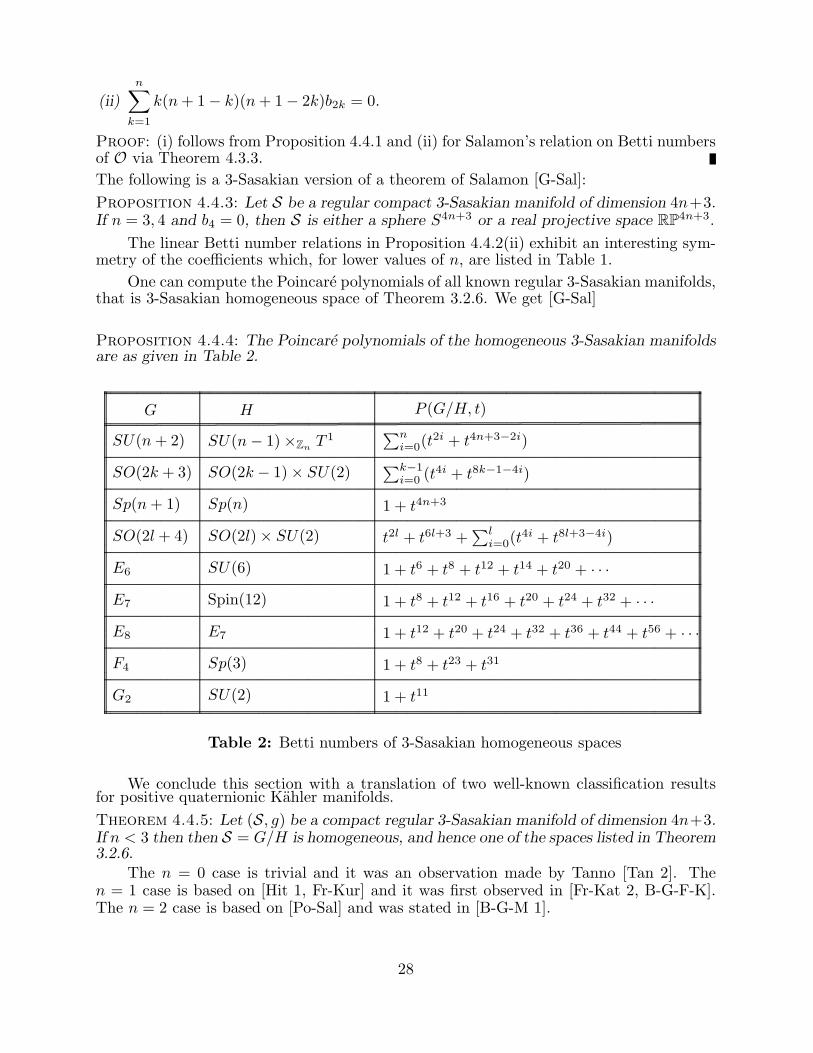
(ii)

n∑

k=1

k(n+ 1− k)(n+ 1− 2k)b2k = 0.

Proof: (i) follows from Proposition 4.4.1 and (ii) for Salamon’s relation on Betti numbersof O via Theorem 4.3.3.

The following is a 3-Sasakian version of a theorem of Salamon [G-Sal]:

Proposition 4.4.3: Let S be a regular compact 3-Sasakian manifold of dimension 4n+3.If n = 3, 4 and b4 = 0, then S is either a sphere S4n+3 or a real projective space RP4n+3.

The linear Betti number relations in Proposition 4.4.2(ii) exhibit an interesting sym-metry of the coefficients which, for lower values of n, are listed in Table 1.

One can compute the Poincare polynomials of all known regular 3-Sasakian manifolds,that is 3-Sasakian homogeneous space of Theorem 3.2.6. We get [G-Sal]

Proposition 4.4.4: The Poincare polynomials of the homogeneous 3-Sasakian manifoldsare as given in Table 2.

..........................................................................................................................................................................................................................................................................................................................................................................................................................................................................................................................

..........................................................................................................................................................................................................................................................................................................................................................................................................................................................................................................................

..........................................................................................................................................................................................................................................................................................................................................................................................................................................................................................................................

..........................................................................................................................................................................................................................................................................................................................................................................................................................................................................................................................

..........................................................................................................................................................................................................................................................................................................................................................................................................................................................................................................................

..........................................................................................................................................................................................................................................................................................................................................................................................................................................................................................................................

....................................................................................................................................................................................................................................................................................................................................................................................................................................................................................................................................................................................................................................................................................................................................................................................................................................................................................................................................................................................................................................................................................................................................................................................................................................................................................................................................................................................................................................................................................................................................................................................................................................................................................................................................................................................................................................................................................................................................................

G H P (G/H, t)....................................................................................................................................................................................................................................................................................................................................................................................................................................................................................................................................................................................................................................................................................................................................................................................................................................................................................................................................................................................................................................................................................................................................................................................................................................................................................................................................................................................................................................................................................................................................................................................................................................................................................................................................................................................................................................................................................................................................................

SU(n+ 2) SU(n− 1)×ZnT 1

∑ni=0(t

2i + t4n+3−2i)..........................................................................................................................................................................................................................................................................................................................................................................................................................................................................................................................................................................................................................................................................................................................................................................................................................................................................................................................................................................

SO(2k + 3) SO(2k − 1)× SU(2)∑k−1

i=0 (t4i + t8k−1−4i)..........................................................................................................................................................................................................................................................................................................................................................................................................................................................................................................................................................................................................................................................................................................................................................................................................................................................................................................................................................................

Sp(n+ 1) Sp(n) 1 + t4n+3

..........................................................................................................................................................................................................................................................................................................................................................................................................................................................................................................................................................................................................................................................................................................................................................................................................................................................................................................................................................................

SO(2l + 4) SO(2l)× SU(2) t2l + t6l+3 +∑l

i=0(t4i + t8l+3−4i)

..........................................................................................................................................................................................................................................................................................................................................................................................................................................................................................................................................................................................................................................................................................................................................................................................................................................................................................................................................................................

E6 SU(6) 1 + t6 + t8 + t12 + t14 + t20 + · · ·..........................................................................................................................................................................................................................................................................................................................................................................................................................................................................................................................................................................................................................................................................................................................................................................................................................................................................................................................................................................

E7 Spin(12) 1 + t8 + t12 + t16 + t20 + t24 + t32 + · · ·..........................................................................................................................................................................................................................................................................................................................................................................................................................................................................................................................................................................................................................................................................................................................................................................................................................................................................................................................................................................

E8 E7 1 + t12 + t20 + t24 + t32 + t36 + t44 + t56 + · · ·..........................................................................................................................................................................................................................................................................................................................................................................................................................................................................................................................................................................................................................................................................................................................................................................................................................................................................................................................................................................

F4 Sp(3) 1 + t8 + t23 + t31..........................................................................................................................................................................................................................................................................................................................................................................................................................................................................................................................................................................................................................................................................................................................................................................................................................................................................................................................................................................

G2 SU(2) 1 + t11....................................................................................................................................................................................................................................................................................................................................................................................................................................................................................................................................................................................................................................................................................................................................................................................................................................................................................................................................................................................................................................................................................................................................................................................................................................................................................................................................................................................................................................................................................................................................................................................................................................................................................................................................................................................................................................................................................................................................................

Table 2: Betti numbers of 3-Sasakian homogeneous spaces

We conclude this section with a translation of two well-known classification resultsfor positive quaternionic Kahler manifolds.

Theorem 4.4.5: Let (S, g) be a compact regular 3-Sasakian manifold of dimension 4n+3.If n < 3 then then S = G/H is homogeneous, and hence one of the spaces listed in Theorem3.2.6.

The n = 0 case is trivial and it was an observation made by Tanno [Tan 2]. Then = 1 case is based on [Hit 1, Fr-Kur] and it was first observed in [Fr-Kat 2, B-G-F-K].The n = 2 case is based on [Po-Sal] and was stated in [B-G-M 1].

28

5. Killing Spinors and G2-Structures

In this section we discuss some additional properties of Sasakian and Sasakian-Einsteinmanifolds which are connected with spin structure and eigenvalues of the Dirac operator

5.1 Killing Spinors

Definition 5.1.1: Let (M, g) be a complete n-dimensional Riemannian spin manifold,and let S(M) be the spin bundle of M and ψ a smooth section of S(M). We say that ψis a Killing spinor if

5.1.2 ∇Xψ = α·X ·ψ, ∀X ∈ Γ(TM),

where ∇ is the Levi-Civita connection of g and X ·ψ denotes the Clifford product of Xand ψ. We say that ψ is imaginary when α ∈ Im(C∗), ψ is parallel if α = 0 and ψ is realif α ∈ Re(C∗).

From the point of view of Einstein geometry the importance of Killing spinors is animmediate consequence of the following theorem of Friedrich [Fr]:

Theorem 5.1.2: Let (M, g) be an n-dimensional; complete Riemannian spin manifoldwith a Killing spinor. Then M is Einstein with Einstein constant λ = 4(n − 1)α2. Inparticular, when α ∈ Re(C∗), M is compact of positive scalar curvature.

On the other hand, Friedrich showed that if M is a compact spin manifold of positivescalar curvature and R0 is the minimum of the scalar curvature, then for all eigenvaluesβ of the Dirac operator D one has β2 ≥ 1

4nR0

n−1 [Fr 1]. If the equality holds than it follows

that the corresponding eigenspinor must be a Killing spinor with α = ±12 [ R0

n(n−1) ]1/2. We

have the following important property of manifolds with Killing spinors [B-G-F-K]:

Theorem 5.1.3: Let (Mn, g) be a connected Riemannian spin manifold admitting a non-trivial Killing spinor with α 6= 0. Then (M, g) is locally irreducible. Furthermore, if M islocally symmetric, or n ≤ 4, then M is a space of constant sectional curvature equal 4α2.

From now on we will be interested only in the case of real Killing spinors. It wasFriedrich and Kath [Fr-Kat 1-2] who first noticed that in some low odd dimensions theexistence of real Killing spinors leads naturally to the existence of Sasakian-Einstein or3-Sasakian structures. Later, the problem found a simple classification in terms of theholonomy of the associated metric cone C(M) [Bar]. First, we have the following definition:

Definition 5.1.4: We say that M is of type (p, q) if it carries exactly p linearly indepen-dent real Killing spinors with α > 0 and exactly q linearly independent real Killing spinorswith α < 0, or vice versa.

For, example, the standard sphere Sn is of type (2[n/2], 2[n/2]). Bar shows that whenM admits a real Killing spinor then the cone (C(M), g) has a parallel spinor. In particular,C(M) is always Ricci-flat and, when M is simply-connected, then only a few holonomygroups Hol(g) are possible [Wan 3]:

Theorem 5.1.5: Let (Mn, g) be a simply-connected Riemannian spin manifold admittinga non-trivial Killing spinor and let Hol(g) be the holonomy group of the metric cone(C(M), g). Then there are only the following 6 possibilities for the triple

(

n,Hol(g), (p, q))

:

(1) n arbitrary, Hol(g) = id, (p, q) = (2[n/2], 2[n/2]),(2) n = 2m+ 1, m even, Hol(g) = SU(m+ 1), (p, q) = (1, 1),

29

(3) n = 4m+ 3, Hol(g) = SU(2m+ 2), (p, q) = (2, 0),(4) n = 4m+ 3, Hol(g) = Sp(m+ 1), (p, q) = (m+ 2, 0),(5) n = 7, Hol(g) = Spin(7), (p, q) = (1, 0),(6) n = 6, Hol(g) = G2, (p, q) = (1, 1).

The first case is special as M is the n-dimensional round sphere. Since M is assumedto be simply-connected, in the next two cases, by Proposition 1.1.9, M must be Sasakian-Einstein. In the case (4), by Definition 1.2.1, M is 3-Sasakian. Specifically, we get thefollowing theorem [Bar]:

Theorem 5.1.6: Let (Mn, g) be a complete simply-connected Riemannian spin manifoldadmitting a non-trivial Killing spinor with α > 0 or α < 0. If n = 2m + 1, m ≥ 2 even,then there are two possibilities:

(i) (M, g) = (Sn, gcan),

(ii) (M, g) is of type (1, 1) and it is a Sasakian-Einstein manifold.

Conversely, if (M, g) is a complete simply-connected Sasakian-Einstein manifold ofdimension 4m+ 1, then M carries Killing spinors with α > 0 and α < 0.

Remark 5.1.7: Note that in the converse statement we do not need to assume that M isspin. When π1(M) = 0 this is automatic by Corollary 1.1.11. When π1(M) 6= 0 then the‘if’ part of Theorem 5.1.6 can be generalized and we still get two possibilities: (i) either Mis a spin spherical space form, or (ii) it is of type (1, 1) with a Sasakian-Einstein structureand Hol(g) = SU(m+ 1) [Wan 3].

Theorem 5.1.8: Let (Mn, g) be a complete simply-connected Riemannian spin manifoldadmitting a non-trivial Killing spinor with α > 0 or α < 0. If n = 4m + 3, m ≥ 2, thenthere are three possibilities:

(i) (M, g) = (Sn, gcan),

(ii) (M, g) is a Sasakian-Einstein manifolds of type (2, 0), but (M, g) is not 3-Sasakian,

(iii) (M, g) is of type (m+ 2, 0) and it is 3-Sasakian.

Conversely, if (M, g) is a complete simply-connected 3-Sasakian manifold, of dimen-sion 4m+3 which is not of constant curvature, then M carries (m+2) linearly independentKilling spinors with α > 0. If (M, g) is a complete simply-connected Sasakian-Einsteinmanifold of dimension 4m+3 which is not 3-Sasakian thenM carries 2 linearly independentKilling spinors with α > 0.

Remark 5.1.9: Note that in Theorem 5.1.8(ii) we are not excluding the possibility ofM having another 3-Sasakian structure with a different metric g′. We are only sayingthat the holonomy group Hol(g) = SU(2m + 2) rather than Sp(m + 1) ⊂ SU(2m + 2),which, by definition, means that g cannot be 3-Sasakian. However, we are not aware ofany such example. We have excluded dim(M) = 7 because in this case we have one morepossibility due to Theorem 5.1.5 and we want to discuss the associated geometry in moredetail later. Again, one can generalize Theorems 5.1.8 to π1(M) 6= 0. For the full list ofpossible holonomy groups Hol(g) see [Wan 2]. The coresponding M are then only locallySasakian-Einstein or locally 3-Sasakian [Or-Pi, Pi]. The problem of the existence of Killingspinors on a Sasakian-Einstein or 3-Sasakian manifold with π1(M) 6= 0 is, however, moresubtle.Corollary 5.1.10: Let (S, g) be a compact Sasakian-Einstein manifold of dimension2m+ 1. Then S is locally symmetric if and only if S is of constant curvature. Moreover,(S, g) is locally irreducible as a Riemannian manifold.

30

Proof: If necessary, go to the universal cover S. This is a compact simply-connectedSasakian-Einstein manifold; hence, it admits a non-trivial Killing spinor by Theorems5.1.6 and 5.1.8. The statement then follows from the Theorem 5.1.3.

Corollary 5.1.11: Let (S, g) be a compact Sasakian-Einstein manifold of dimension2m+ 1. Then Hol(g) = SO(2m+ 1).

Proof: Let us consider universal cover S. This is a compact simply-connected Sasakian-Einstein manifold; hence, it admits a non-trivial Killing spinor. By the previous corollary,it can be symmetric if only if it is isomorphic to a space of constant curvature, thatis, a sphere. Then S is a spherical space form and Hol(g) = SO(2m + 1). Assume Sis not locally symmetric. By Corollary 5.1.10 S is locally Riemannian irreducible, so fordimensional reasons and Berger’s famous classification theorem [Ber], the only possibilitiesfor the restricted holonomy group Hol0(g) are SO(2m + 1) and G2 in dimension 7. ButG2 holonomy implies Ricci-flat and, hence, not Sasakian-Einstein. Hence, the restrictedholonomy group Hol0(g) = SO(2m + 1). Since S is orientable this coincides with theholonomy group Hol(g).

5.2 G2-Structures

Recall, that geometrically G2 is defined to be the Lie group acting on R7 and pre-serving the 3-form5.2.1ϕ = α1∧α2∧α3+α1∧(α4∧α5−α6∧α7)+α2∧(α4∧α6−α7∧α5)+α3∧(α4∧α7−α5∧α6),

where αi7i=1 is a fixed orthonormal basis of the dual of R7. A G2 structure on a 7-manifold M is, by definition, a reduction of the structure group of the tangent bundle toG2. This is equivalent to the existence of a global 3-form ϕ ∈ Ω3(M) which may be writtenlocally as 5.2.1. Such a 3-form defines an associated Riemannian metric, an orientationclass, and a spinor field of constant length. The following terminology is due to Gray [Gra2]:

Definition 5.2.2: Let (M, g) be a complete 7-dimensional Riemannian manifold. We saythat that (M, g) has weak holonomy G2 if there exist a global 3-form ϕ ∈ Ω3(M) whichlocally can be written in terms of a local orthonormal basis as in 5.2.1, and dϕ = c ⋆ ϕ,where ⋆ is the Hodge star operator associated to g and c is a constant whose sign is fixedby an orientation convention.

The equation dϕ = c ⋆ ϕ implies that ϕ is ‘nearly parallel’ in the sense that only a 1-dimensional component of ∇ϕ is different from zero [Fe-Gra]. Thus, a weak holonomy G2

structure is sometimes called a nearly parallel G2 structure. The case of c = 0 is somewhatspecial. In particular, it is known [Sal 4] that the condition dϕ = 0 = d ⋆ ϕ is equivalentto the condition that ϕ be parallel, i.e., ∇ϕ = 0 which is equivalent to the condition thatthe metric g has holonomy group contained in G2. For a discussion of this very interestingand very difficult case, see the article by D. Joyce in this volume. The following theoremprovides the connection with the previous discussion on Killing spinors [Bar]

Theorem 5.2.3: Let (M, g) be a complete 7-dimensional Riemannian manifold with weakholonomy G2. Then the holonomy group Hol(g) of the metric cone (C(M), g) is containedin Spin(7). In particular, C(M) is Ricci-flat and M is Einstein with positive Einsteinconstant λ = 6.Remark 5.2.4: The sphere S7 with its constant curvature metric is isometric to theisotropy irreducible space Spin(7)/G2. The fact that G2 leaves invariant (up to constants)a unique 3-form and a unique 4-form on R7 implies immediately that this space has weakholonomy G2.

31

Definition 5.2.5: Let (M, g) be a complete 7-dimensional Riemannian manifold. We saythat g is a proper G2-metric if Hol(g) = Spin(7).

Theorem 5.2.6: Let (M7, g) be a complete simply-connected Riemannian spin manifoldof dimension 7 admitting a non-trivial Killing spinor with α > 0 or α < 0. Then there arefour possibilities:

(i) (M, g) is of type (1, 0) and it is a proper G2-manifold,

(ii) (M, g) is of type (2, 0) and it is a Sasakian-Einstein manifold, but (M, g) is not 3-Sasakian,

(iii) (M, g) is of type (3, 0) and it is 3-Sasakian,

(iv) (M, g) = (S7, gcan) and is of type (8, 8).

Conversly, if (M, g) is a compact simply-connected proper G2-manifold then it carriesa Killing spinor with α > 0. If (M, g) is a compact simply-connected Sasakian-Einstein7-manifold which is not 3-Sasakian then M carries 2 linearly independent Killing spinorswith α > 0. Finally, if (M, g) is a 3-Sasakian 7-manifold, which is not of constant curvature,then M carries 3 linearly independent Killing spinors with α > 0.

Remark 5.2.7 The four possibilities of the Theorem 5.2.6 correspond to the sequence ofinclusions

Spin(7) ⊃ SU(4) ⊃ Sp(2) ⊃ id.All of the corresponding cases are examples of weak holonomy G2 metrics. If we excludethe trivial case when the associated cone is flat, we have three types of the weak holonomyG2 geometries. Following [F-K-M-S] we use the number of linearly independent Killingspinors to classify the types of weak holonomy G2 geometries. We call these type I, II,and III corresponding to cases (i), (ii), and (iii) of Theorem 5.2.6, respectively.

Remark 5.2.8 In the case π1(M) 6= 0, then M is either a spin spherical space form orHol(g) equals to SU(4), SU(4)>⊳ Z2, Sp(2), or Spin(7) of type (2, 0), (1, 0), (3, 0), (1, 0),respectively. Hence, we have just one more possible geometry for M [Wan 3]. Note thatin the case Hol(g) = SU(4)>⊳ Z2, the cone C(M) is not Kahler so that M cannot beSasakian, but it is locally so.

Recall that S7, regarded as the space Sp(2)/Sp(1) and fibering over S4, admits a‘squashed’ Einstein metric which does not have constant curvature. This metric also hasweak holonomy G2 since the associated cone metric has holonomy equal to Spin(7) andtherefore S7 with this metric is a proper G2-manifold. We can generalize this example toget [G-Sal, F-K-M-S]:

Theorem 5.2.9: Let (S, g) be a 7-dimensional 3-Sasakian manifold. Then the metric ghas weak holonomy G2. Moreover, the second Einstein metric g′ given by Theorem 2.4.2has weak holonomy G2. In fact g′ is a proper G2 metric.

Proof: For the second Einstein metric g′ we have three mutually orthonormal 1-formsα1 =

√tη1, α2 =

√tη2, α3 =

√tη3, where t is the parameter of the canonical variation

discussed in section 2.4. Let α4, α5, α6, α7 be local 1-forms spanning the annihilator ofV3 in T ∗S such that

Φ1 = 2(α4 ∧ α5 − α6 ∧ α7),

Φ2 = 2(α4 ∧ α6 − α7 ∧ α5),

Φ3 = 2(α4 ∧ α7 − α5 ∧ α6).

32

Then the set α1, · · ·α7 forms a local orthonormal coframe for the metric g′. In terms of

the 3-forms Υ and Θ of 4.2.2 we have ϕ = 12

√tΘ +

√t3Υ. One easily sees that this is of

the type of Equation 5.2.1 and, therefore, defines a compatible G2-structure. Moreover, astraightforward computation gives

dϕ =1

2

√tΩ +

√t(t+ 1)dΥ, ⋆ϕ = −1

2tdΥ− 1

24Ω.

Thus, dϕ = c ⋆ ϕ is solved with√t = 1/

√5, and c = −12/

√5. So g′ has weak holonomy

G2. That g′ is a proper G2 metric is due to [F-K-M-S]. The idea is to use Theorem 5.2.6.Looking at the four possibilities given in that theorem, we see that it suffices to show thatg′ is not Sasakian-Einstein. The details are in [F-K-M-S].

Examples 5.2.10: 3-Sasakian 7-manifolds are plentiful and examples will be discussedin next section. These give, by Theorem 5.2.9, many examples of type I and type III ge-ometries. Examples of simply-connected type I geometries that do not arise via Theorem5.2.9 are the homogeneous Aloff-Wallach spaces Nk,l = SU(3)/T 1

k,l, with gcd(k, l) = 1 and

(k, l) 6= (1, 1) [C-M-Sw, B-G-F-K] together with the homogeneous real Stiefel manifoldSO(5)/SO(3) [Bry]. All the known type II geometries are the 3 homogeneous exam-ples from the list of Corollary 3.1.3(iii) (not 3-Sasakian) and the inhomogeneous simply-connected circle bundles over Pk ×CP1, where Pk is the del Pezzo surface with 2 < k < 9[F-K-M-S]. Actually, N1,1 has three Einstein metrics. One is 3-Sasakian and is denoted byS(1, 1, 1) in section 7.4 below. The second is the proper G2 metric of Theorem 5.9, whilethe third Einstein metric also has weak holonomy G2 most likely of type I but we couldnot positively exclude type II as a possibility [C-M-Sw].

6. The Quotient Construction

In this section we give a general 3-Sasakian reduction procedure which constructs new3-Sasakian manifolds from a given 3-Sasakian manifold S with a non-trivial 3-Sasakianisometry group I0(S, g) [B-G-M 2]. Actually, this is a reduction that is associated witha quadruple of spaces of the fundamental diagram ♦(S). At the level of the hyperkahlercone C(S) the reduction was discovered by Lindstrom and Rocek [L-R] in the context ofsupersymmetric σ-model and later rigorously described by Hitchin et al. in [H-K-L-R]. Inthe case of the quaternionic Kahler base O the reduction was discovered by the secondauthor and H.B. Lawson [G, G-L]. The lift of the quaternionic Kahler quotient to thetwistor space Z was described by Hitchin [Hit 2]. In this section we restrict ourselves todescribing the general procedure of reduction together with the homogeneous case arisingfrom reduction by a circle group, as well as a brief discription of the singular case. Thelarge class of 3-Sasakian toric manifolds obtained by reduction is relagated to a separatesection, namely section 7. It should also be understood that every 3-Sasakian reductiongives as well a reduction procedure for each of the spaces of the fundamental diagram♦(S).

6.1. The 3-Sasakian Moment Map

Let (S, g) be a 3-Sasakian manifold with a nontrivial group I0(S, g) of 3-Sasakianisometries. By the Definition 1.2.1, C(S) = S×R+ is a hyperkahler manifold with respectto the cone metric g. The isometry group I0(S, g) extends to a group I0(C(S), g) ∼= I0(S, g)of isometries on C(S) by defining each element to act trivially on R+. Furthermore, itfollows easily from the definition of the complex structures Ia given in equation 1.1.7

33

that these isometries I0(C(S), g) are hyperkahler; that is, they preserve the hyperkahlerstructure on C(S). Recall [H-K-L-R] shows that any subgroup G ⊂ I0(M, g) gives rise toa hyperkahler moment map µ : M−→g∗⊗R3, where g denotes the Lie algebra of G and g∗

is its dual. Thus, we can define a 3-Sasakian moment map

6.1.1 µS : S −−→ g∗ ⊗ R3

by restriction µS = µ | S. We denote the components of µS with respect to the standardbasis of R3, which we have identified with the imaginary quaternions, by µa

S . Recall thatordinarily moment maps determined by Abelian group actions (in particular, those asso-ciated to 1-parameter groups) are only specified up to an arbitrary constant. This is notthe case for 3-Sasakian moment maps since we require that the group Sp(1) generatedby the Sasakian vector fields ξa acts on the level sets of µS . However, we shall see that3-Sasakian moment maps are given by a particularly simple expression.

Proposition 6.1.2: Let (S, g) be a 3-Sasakian manifold with a connected compact Liegroup G acting on S by 3-Sasakian isometries. Let τ be an element of the Lie algebra gof G and let Xτ denote the corresponding infinitesimal isometry. Then there is a unique3-Sasakian moment map µS such that the zero set µ−1

S (0) is invariant under the groupSp(1) generated by the vector fields ξa. This moment map is given by

6.1.3 < µaS , τ > =

1

2ηa(Xτ).

Furthermore, the zero set µ−1S (0) is G invariant.

Proof: Using the Definition 1.2.1 we can define the 2-forms ωaS on S as the restriction of

the hyperkahler 2-forms ωa. Then any 3-Sasakian moment map µaS(τ) determined by τ ∈ g

satisfies 2dµaS(τ) = 2Xτ⌋ωa

S = −Xτ⌋dηa. As Xτ is a 3-Sasakian infinitesimal isometry,Lemma 3.2.2 implies that 2 < µa

S , τ > differs from ηa(Xτ) by a constant depending on a

and τ. One then uses the invariance of the zero set µ−1S (0) to show that these constants

must vanish. See [B-G-M 2] for details.

Henceforth by the 3-Sasakian moment map, we shall mean the moment map µSdetermined in Proposition 6.1.2. Hence, the Definition 1.2.1 and Proposition 6.1.2 imply

Theorem 6.1.5: Let (S, g) be a 3-Sasakian manifold with a connected compact Liegroup G acting on S smoothly and properly by 3-Sasakian isometries. Let µS be thecorresponding 3-Sasakian moment map and assume both that 0 is a regular value of µS

and that G acts freely on the submanifold µ−1S (0). Furthermore, let ι : µ−1

S (0)−−→Sand π : µ−1

S (0)−−→µ−1S (0)/G denote the corresponding embedding and submersion. Then

(S///G = µ−1S (0)/G, g) is a smooth 3-Sasakian manifold of dimension 4(n−dim g)+3 with

metric g and characteristic vector fields ξa determined uniquely by the two conditionsι∗g = π∗g and π∗(ξ

a |µ−1S (0)) = ξa.

We conclude this part with the following fact concerning 3-Sasakian isometries whoseproof can be found in [B-G-M2].

Proposition 6.1.6: Assume that the hypothesis of Theorem 6.1.5 holds. In additionassume that (S, g) is complete and hence compact. Let C(G) ⊂ I0(S, g) denote thecentralizer of G in I0(S, g) and let C0(G) denote the subgroup of C(G) given by theconnected component of the identity. Then C0(G) acts on the submanifold µ−1

S (0) asisometries with respect to the restricted metric ι∗g and the 3-Sasakian isometry group

34

I0(S///G, g) of the quotient (S///G, g) determined in Theorem 6.1.5 contains an isomorphiccopy of C0(G). Furthermore, if C0(G) acts transitively on S///G, then S///G is a 3-Sasakianhomogeneous space.

It should be mentioned that it is not required that the isometry group I0(S///G, g)acts effectively.

6.2 Regular Quotients And Classical Homogeneous Metrics

We now apply the reduction procedure given in Theorem 6.1.4 to the round unitsphere S4n+3 to explicitly construct the Riemannian metrics for the 3-Sasakian homoge-neous manifolds arising from the simple classical Lie algebras. These metrics are preciselythe ones associated to the three infinite families appearing in Theorem 3.2.6. The quo-tient construction applied to ♦(S4n+3) explicitly describes all metrics in the fundamentaldiagrams ♦(G/H), where G is either the special unitary SU(n + 1) or the orthogonalgroup SO(n + 1). To carry out this reduction we must set some conventions. We de-scribe the unit sphere S4n+3 by its embedding in flat space and we represent an elementu = (u1, · · · , un+1) ∈ Hn+1 as a column vector. The quaternionic components of thisvector are denoted by u0 for the real component and by ua for the three imaginary com-ponents so that we can write u = u0+iu1+ju2+ku3 using the quaternionic units i, j, k.We also define quaternionic conjugate u = u0 − iu1 − ju2 − ku3.

Now, the infinitesimal generators of the subgroup Sp(1) ⊂ H∗ acting by the rightmultiplication on u are the defining vector fields ξa for the Sasakian 3-structure. Thesevector fields are given by

6.2.1 ξar = u0 · ∂

∂ua− ua · ∂

∂u0− ǫabcub · ∂

∂uc,

where the dot indicates sum over the vector components ui and the subscript r meansthat these vector fields are the generators of the right action.

We will first consider G = U(1) acting on the sphere S4n+3 as follows

6.2.2 ϕt(u) = τu, τ = e2πit, u ∈ S4n+3.

Note that this action is actually free on S4n+3 and hence it will be automatically free onthe level set of the moment map. To compute the moment map we identify the imaginaryquaternions R3 with the Lie algebra sp(1) in equation 6.1.1 and the Lie algebra of U(1)with R, so the moment map is µS : S4n+3 −−→ R⊗ sp(1) and it can easily be computed

6.2.3 µS(u) =

n+1∑

α=1

uαiuα.

One can easily identify the zero-level set of the moment map with the Stiefel manifold ofcomplex 2-frames in Cn+1, and the following proposition is then an immediate consequenceof Theorem 6.1.5.

Proposition 6.2.4: Let N = µ−1S (0) and ι : N → S4n+3 be the inclusion. Then ι

is an embedding and (N, ι∗gcan) is the complex homogeneous Stiefel manifold V C2,n+1 =

SU(n+1)/SU(n−1) of 2-frames in Cn+1. Hence, the 3-Sasakian quotient S4n+3///U(1) =

35

V C2,n+1/U(1) = SU(n + 1)/S(U(n − 1) × U(1)) with the 3-Sasakian metric g given by

inclusion ι and submersion π : N −−→ N/U(1), i.e., ι∗gcan = π∗g.

Remark 6.2.5: A similar construction can be carried out for the Sp(1)-action on S4n+3

defined by the left multiplication of u by a unit quaternion σ, i.e.,

6.2.6 ϕσ(u) = σu, σσ = 1, u ∈ S4n+3.

This action is free on S4n+3 and the zero-level set of the corresponding moment map canbe easily identified with the real Stiefel manifold V R

4,n+1 ≃ SO(n+1)/SO(n−3) of 4-frames

in Rn+1 with n ≥ 4. Hence, the reduced space S4n+3///Sp(1) = SO(n+1)SO(n−3)×Sp(1) . For the

more detailed and uniform description of the geometry of these two quotients see [B-G-M2].

6.3 The Structure of Singular Quotients

In this section we will describe a more general situation, when the zero-level set ofthe 3-Sasakian moment map 6.1.1 is not necessarily smooth and the group action on thelevel set is not necessarily locally free.

Let G be a Lie group acting smoothly and properly on a manifold S and let H ⊂ Gbe a subgroup. Using standard notation we will denote by SH ⊂ S the set of points in Swhere the stability group is exactly equal to H and by S(H) ⊂ S the set of points withstabilizer conjugate to H in G. It follows than that the normalizer N(H) of H in G actsfreely on S(H). Then we have the following theorem due to Dancer and Swann [D-Sw]:

Theorem 6.3.1: Let (S, g) be a 3-Sasakian manifold with a connected compact Lie groupG acting on S smoothly and properly by 3-Sasakian isometries. Let µS be the corre-sponding 3-Sasakian moment map. Then the quotient µ−1

S (0)/G is a union of the smooth,

3-Sasakian manifolds (S(H) ∩ µ−1S (0))/G, where (H) runs over the conjugacy classes of

stabilizers of points in S.

Quite often S(H) does not meet the zero locus of the moment map. Then the stratum

(S(H) ∩ µ−1S (0))/G is empty.

Example 6.3.2: We start with the 3-Sasakian sphere S4n+3 in the notation of the previoussection. But now we consider a different circle action U(1), namely

ϕp,q;mt (u) = (τpu1, . . . , τ

pum, τqum+1, . . . , τ

qun+1), τ = e2πit, u ∈ S4n+3,

where 0 ≤ m ≤ n+ 1 and p, q ∈ Z. Let S(p, q;m) = S4n+3///U(1) be the quotient.

(i) First, let p, q be relatively prime positive integers bigger than 1 and 2 ≤ m ≤ n− 1.Then, the stratified manifold S(p, q;m) consists of 3 strata. The stratum of the highestdimension corresponding toH = id is an open incomplete 3-Sasakian manifold. Thetwo strata of lower dimension are easily seen to be the homogeneous spaces: one withH = Zq is the homogeneous 3-Sasakian space of SU(n + 1 − m) and the one withH = Zp is the homogeneous 3-Sasakian space of SU(m). In this case, S(p, q;m)is actually a compact 3-Sasakian orbifold and the stratification of Theorem 6.3.1coincides with the orbifold stratification.

(ii) Consider S(0, p;m), where p > 1 and 2 ≤ m ≤ n− 1. There are two strata now: thestratum of the highest dimension corresponds to H = Zp and the second stratum is

36

just the sphere S4m−1 with H = U(1). The space S(0, p;m) is not an orbifold but,as pointed out in [D-Sw], it does have a length space structure.

(iii) Consider S(0, 1;n). Here H is either U(1) or trivial but the set S4n+3id does not

meet the zero locus of the moment map. Hence, there is only one stratum andS(0, 1;n) = S4n−1.

(iv) Finally, consider S(0, 1;n− 1). The stability group H is either U(1) or trivial. Thestratum corresponding to H = U(1) is the sphere S4n−5. We leave it as an exerciseto the reader to show that S(0, 1;n− 1) is an orbifold and that it can be identifiedwith S4n−1/Z2, where (w1, ...., wn) ∈ S4n−1, where Z2 acts on the last quaternioniccoordinate by multiplication by ±1.

7. Toric 3-Sasakian Manifolds

In this section we shall describe the quotient construction of large families of 3-Sasakian manifolds S(Ω). They all have the property that I0(S(Ω), g(Ω)) ⊃ Tm, wheredim(S(Ω)) = 4m−1, and following the ideas of [Bi-D] we shall call such 3-Sasakian mani-folds toric (See 7.6.1 for a precise definition). We also describe some interesting geometricand topological properties of such spaces. Up until now all known examples of 3-Sasakianmanifolds are either homogeneous or toric or discrete quotients of them.

7.1 Toral Reductions of Spheres

Using the notation of the previous section we start with the unit (4n+3)-dimensionalsphere embedded in the quaternionic vector space Hn+1. The subgroup of the full isometrygroup O(4n+ 3) that preserves the quaternionic structure is Sp(n+ 1)·Sp(1) acting by

7.1.1 ϕA,σ(u) = Auσ−1,

where A ∈ Sp(n + 1) is the quaternionic (n + 1) × (n + 1) matrix of the quaternionicrepresentation of Sp(n + 1), and σ ∈ Sp(1) is a unit quaternion. As the diagonal Z2

acts trivially this is indeed an Sp(n + 1) ·Sp(1) action. The group Sp(n + 1) is thesubgroup of Sp(n + 1) ·Sp(1) which preserves the 3-Sasakian structure on S4n+3, so wehave I0(S

4n+3, gcan) = Sp(n+1). We shall consider the maximal torus Tn+1 ⊂ Sp(n+ 1)and its subgroups. Every quaternionic representation of a k-torus T k on Hn+1 can be

described by an exact sequence 0−−→T kfΩ−−→Tn+1−−→Tn+1−k−−→0. The monomorphism fΩ

can be represented by the matrix

7.1.2 fΩ(τ1, . . . , τk) =

k∏

i=1

τai1

i . . . 0

.... . .

...

0 . . .k∏

i=1

τai

n+1

i

,

where (τ1, .., τk) ∈ S1 × · · · × S1 = T k are the complex coordinates on T k, and aij ∈ Z are

the coefficients of a k × (n+ 1) integral weight matrix Ω = (alα)l=1,...,k

α=1,...,n+1 ∈Mk,n+1(Z).

37

Let elkl=1 denote the standard basis for t∗k ≃ Rk. Then the 3-Sasakian moment mapµΩ : S4n+3−−→t∗k ⊗ R3 of the k-torus action defined by ϕ(τ1,...,τk)(u) = fΩ(τ1, . . . , τk)u, is

given by µΩ =∑

l µlΩel with

7.1.3 µlΩ(u) =

∑

α

uαialαuα.

Let us further denote the triple (T k, fΩ, ϕ(τ1,...,τk)) by T k(Ω).

Definition 7.1.4: N(Ω) = µ−1Ω (0) and S(Ω) = S4n+3///T k(Ω) = N(Ω)/T k(Ω).

Let S4n+3H denote all the points on the sphere where the stability group H ⊂ T k is

exactly H. Because T k is Abelian S4n+3H = S4n+3

(H) . Furthermore, let KH = T k/H and

denote by S(Ω;H) = S4n+3H ∩N(Ω)/KH . Following Theorem 6.3.1 we have

Proposition 7.1.5: The quotient S(Ω) =⋃

H S(Ω;H) is a disjoint union of 3-Sasakianmanifolds, where each stratum S(Ω;H) is smooth.

We will be interested in the case when S(Ω) is a compact orbifold (all stability groupsH for which S4n+3

H ∩ N(Ω) are non-empty are discrete) or a compact smooth manifold(there is only one stratum). Necessary and sufficient conditions for this to happen canbe expressed in terms of properties of the matrix Ω. First observe that, without loss ofgenerality, we can assume that the rank of Ω equals k. Otherwise, one simply has anaction of a torus of lower dimension and the whole problem reduces to considering anotherweight matrix Ω with fewer rows.

We introduce the following terminology: Consider the(

nk

)

minor determinants

7.1.6 ∆α1...αk= det

a1α1

. . . a1αk

......

akα1

. . . akαk

obtained by deleting n+ 1− k columns of Ω.

Definition 7.1.7: Let Ω ∈Mk,n+1(Z) be the weight matrix.

(i) If ∆α1······αk6= 0, ∀ 1 ≤ α1 < · · · < αk ≤ n+1, then we say that Ω is non-degenerate.

Suppose Ω is non-degenerate and let g be the kth determinantal divisor, i.e., the gcdof all the k by k minor determinants ∆α1······αk

. Then Ω is said to be admissible if inaddition we have(ii) gcd(∆α2···αk+1

, ...,∆α1···αs···αk+1, ...,∆α1···αk

) = g for all sequences of length (k+1)such that 1 ≤ α1 < · · · < αs < · · · < αk+1 ≤ n+ 1.

7.2 Equivalence Problem and Admissibility

Before we show how these properties of the matrix Ω impact on the geometry of thequotient S(Ω) we need to discuss the notion of the equivalence of T k-actions on S4n+3

and obtain a normal form for admissible weight matrices. We are free to change basesof the Lie algebra tk. This can be done by the group of unimodular matrices GL(k,Z).Moreover, if we fix a maximal torus Tn+1 of Sp(n + 1), its normalizer, the Weyl groupW(Sp(n+ 1)) ≃ Σn+1 >⊳ (Z2)

n+1, preserves the 3-Sasakian structure on S4n+3 and inter-twines the T k actions. Thus, there is an induced action of GL(k,Z) ×W(Sp(n + 1)) on

38

the set of weight matricesMk,n+1(Z). The group GL(k,Z) acts onMk,n+1(Z) by matrixmultiplication from the left, and the Weyl group W(Sp(n+ 1)) acts by permutation andoverall sign changes of the columns. Actually we want a slightly stronger notion of equiv-alence than that described above. If the ith row of Ω has a gcd di greater than one, then

by reparameterizing the one-parameter subgroup τ ′i = τdi

i we obtain τaj

α

i = (τ ′i)bi

α , wheregcdbiαα = 1. So the action obtained by using the matrix whose ith row is divided by itsgcd di is the same as the original action. The integers di all divide the kth determinantaldivisor g. We say that a non-degenerate matrix Ω is in reduced form (or simply reduced) ifg = 1. The following easy lemma says that among non-degenerate matrices it is sufficientto consider matrices in a reduced form.Lemma 7.2.1: Every non-degenerate weight matrix Ω is equivalent to a matrix in a reducedform.Henceforth, we shall only consider matrices in a reduced form.

Definition 7.2.2: Let Ak,n+1(Z) ⊂ Mk,n+1(Z) denote the subset of reduced admissiblematrices. This subset is invariant under the action of GL(k,Z) ×W(Sp(n + 1)), so theset Ak,n+1(Z)/GL(k,Z)×W(Sp(n+ 1)) of equivalence classes [Ω] is well defined. We letEk,n+1(Z) ⊂ Ak,n+1(Z) denote a fundamental domain for the action.

Our interest in Ak,n+1(Z) is the following:

Theorem 7.2.3: Let S(Ω) be the quotient space of definition 7.1.6. Then

(i) if Ω is non-degenerate, S(Ω) is an orbifold.

(ii) If Ω is degenerate, then either S(Ω) is a singular stratified space which is not anorbifold or it is an orbifold obtained by reduction of a lower dimensional sphereS4n−4r−1 by a torus T k−r(Ω′) or a finite quotient of such, where 1 ≤ r ≤ k and Ω′ isnon-degenerate. (When r = k the quotient is the sphere S4n−4k−1).

(iii) Assuming that Ω is non-degenerate S(Ω) is a smooth manifold if and only if Ω isadmissible.One can easily see that the non-degeneracy of Ω is not necessary for the quotient

space S(Ω) to be smooth or a compact orbifold (see Example 6.3.3(iv)). However, Theorem7.2.5(ii) shows that then we can reformulate the whole problem in terms of another quotientand a new non-degenerate weight matrix Ω′ and can be found in [B-G-M 7]. Theorem7.2.5(iii) shows then the importance of admissible matrices in the construction and iteasily follows from the fact that non-degeneracy implies that at most n− k quaternioniccoordinates uj can simultaneously vanish on N(Ω) [B-G-M-R 1].

Remark 7.2.4: Our discussion shows clearly that, if Ω,Ω′ ∈ Ak,n+1(Z) such that [Ω] = [Ω′]then the quotients S(Ω) ≃ S(Ω′) are equivalent as 3-Sasakian manifolds. We believe thatthe converse of this is also true, though we will establish it later only in certain cases.

7.3.3 Combinatorics and Admissibility

In general Theorem 7.2.3 is not yet an existence theorem, since Ak,n+1(Z) could beempty. Indeed, for many pairs (k, n) this is the case and we shall demonstrate this next.

Let Ω ∈ Ak,n+1(Z). Since Ω is reduced there is a k by k minor determinant thatis odd. By permuting columns if necessary this minor can be taken to be the first kcolumns. Now consider the mod 2 reduction Mk,n+1(Z)−−→Mk,n+1(Z2). We have the

39

following commutative diagram

7.3.1

GL(k,Z)×Mk,n+1(Z) −−→ Mk,n+1(Z)

y

y

GL(k,Z2)×Mk,n+1(Z2) −−→ Mk,n+1(Z2).

Let Ω ∈ Ak,n+1(Z2) denote the mod 2 reduction of Ω ∈ Ak,n+1(Z). Since the first k by k

minor determinant of Ω is odd, the mod 2 reduction of this minor in Ω is invertible. Thus,we can use the GL(k,Z2) action to put Ω in the form

7.3.2 Ω =

1 0 . . . 0 a1k+1 . . . a1

n+1

0 1 . . . 0 a2k+1 . . . a2

n+1

......

. . ....

... · · ·...

0 0 · · · 1 akk+1 . . . ak

n+1

with aij ∈ Z2.

Lemma 7.3.3: The set Ak,n+1(Z) is empty for n > k + 1 and k > 4.

Proof: The second admissibility condition is equivalent to the condition that every k byk + 1 submatrix of Ω has rank k. By considering k − 1 of the first k columns and 2 oflast n + 1 − k columns, this condition implies (aj

l , ajm) 6= (0, 0) for all j = 1, · · · , k, and

k+ 1 ≤ l < m ≤ n+ 1. Similarly, by considering k− 2 of the first k columns and 3 of lastn+ 1− k columns 7.3.2 implies

7.3.4

(

ail ai

m air

ajl aj

m ajr

)

6=(

1 1 11 1 1

)

,

(

ail ai

m air

ajl aj

m ajr

)

6=(

0 1 10 1 1

)

,

where the last inequality is understood to be up to column permutation. Hence, it followsthat, up to column and row permutations, that any four triples of the last n− k columnsof an admissible Ω must have the form

7.3.5

1 1 10 1 11 0 11 1 0

.

So we see that we cannot add another row without violating the above conditions. Itfollows that k ≤ 4.

Similar analysis shows that

Lemma 7.3.6: The set Ak,n+1(Z) is empty if k > 1 and n− k ≥ 4.

Remark 7.3.7: In view of the above lemmas and the fact that in the remainder of thissection we will be interested only in the smooth and compact quotients we are left withthe following possibilities:

(i) Trivial case of n = k. Then there are many admissible matrices Ω but dim(S(Ω)) = 3and it follows that S(Ω) = S3/Zp, where p = p(Ω) depends on Ω. This case is of littleinterest.

40

(ii) Bi-quotient geometry with k = 1 and n > 1 arbitrary. Here Ω is just a row vector p.The admissibility condition means that the entries are non-zero and pairwise relativelyprime. The quotient S(p) turns out to be a bi-quotient of the unitary group U(n+1)and we shall discuss its geometry and topology in the next subsection.

(iii) The most interesting, 7-dimensional case of k = n − 1. Here one easily sees thatthere are many admissible matrices and we analyze the geometry and topology of thequotients in a separate subsection.

(iv) “Special” quotients: (k, n) = (2, 4), (2, 5), (3, 5), (3, 6), (4, 6), (4, 7). These quotientsare 11- or 15-dimensional and we give examples of admissible weight matrices in eachcase. We shall show also that they provide counterexamples to certain Betti numberrelations that are satisfied in the regular case [G-Sal].

7.4 3-Sasakian Structures on Bi-Quotients

When k = 1 we have Ω = p = (p1, ..., pn+1) and we shall write S(Ω) = S(p),N(Ω) = N(p), fΩ = fp, and τ1 = τ . The quotients S(p) are generalizations of thehomogeneous examples discussed in Section 6.2. We get

A1,n+1(Z) = p ∈ (Z)n+1 | pi 6= 0 ∀i = 1, ..., n+ 1 and gcd(pi, pj) = 1 ∀i 6= j,

E1,n+1(Z) = p ∈ Zn+1 | 0 < p1 ≤ · · · ≤ pn+1 and gcd(pi, pj) = 1 ∀i 6= j.

Note that E1,n+1(Z) can be identified with a certain integral lattice in the positive Weylchamber in t∗n+1.

First, by studying the geometry of the foliations in the diagram ♦(S(p)) [B-G-M 6]one can solve the equivalence problem in this case. We get [B-G-M 3]:

Proposition 7.4.1: Let n ≥ 2 and p,q ∈ A1,n+1(Z) so the quotients S(p) and S(q) aresmooth manifolds. Then S(p) ≃ S(q) are 3-Sasakian equivalent if and only if [p] = [q].

It is easy to see that for p ∈ A1,n+1(Z) the zero locus of the moment map N(p) isalways diffeomorphic to the Stiefel manifold V C

2,n+1 of complex 2-frames in Cn+1. Hence,

the quotient S(p) = V C2,n+1/S

1. We first observe that one can identify V C2,n+1 with the

homogeneous space U(n+ 1)/U(n− 1). Using this identification we have

Proposition 7.4.2: For each p ∈ E1,n+1(Z), there is an equivalence S(p) ≃ U(1)p\U(n+1)/U(n − 1) as smooth U(1)p × U(n − 1)-spaces, where the action of U(1)p × U(n −1) ⊂ U(n+ 1)L × U(n+ 1)R is given by the formula

7.4.3 ϕp

τ,B(W) = fp(τ)W

(

I2 O

O B

)

.

Here W ∈ U(n+ 1) and (τ,B) ∈ S1 × U(n− 1).

Note that the identification S(p) ≃ U(1)p\U(n + 1)/U(n − 1) is only true afterassuming that all the weights are positive, as the right-hand side is not invariant under suchsign changes. Proposition 7.4.2 shows that, in a way, the quotients S(p) can be though ofas “bi-quotient deformation” of the homogeneous model S(1). Now let ιp : N(p) → S4n+3

be the inclusion and πp : N(p) → S(p) be the Riemannian submersion of the momentmap. Then the metric g(p) is the unique metric on S(p) that satisfies ι∗

pgcan = π∗

pg(p).

Using the geometry of the inclusion ιp one can show the following [B-G-M 3,6]

41

Theorem 7.4.4: Let I0(S(p), g(p)) be the group of 3-Sasakian isometries of(

S(p), g(p))

and let k be the number of 1’s in p. Then the connected component of I0 is S(U(k) ×U(1)n+1−k), where we define U(0) = e. Thus, the connected component of the isometrygroup is the product S(U(k) × U(1)n+1−k) × SO(3) if the sums pi + pj are even for all1 ≤ i, j ≤ n+ 1, and S(U(k)× U(1)n+1−k)× Sp(1) otherwise.

In the case that p has no repeated 1’s, the cohomogeneity can easily be determined,viz. [B-G-M 3]

Corollary 7.4.5 : If the number of 1’s in p is 0 or 1 then the dimension of the principalorbit in S(p) equals n + 3 and the cohomogeneity of g(p) is 3n − 4. In particular, the7-dimensional S(p) the family (S(p), g(p)) contains metrics of cohomogeneity 0,1, and 2.

Combining Proposition 7.4.2 with techniques developed by Eschenburg [Esch 1-2] inthe study of certain 7-dimensional bi-quotients of SU(3) one can compute the integralcohomology ring of S(p) [B-G-M 2]:

Theorem 7.4.6: Let n ≥ 2 p ∈ E1,n+1(Z). Then, as rings,

H∗(

S(p),Z) ∼=

(

Z[b2]

[bn+12 = 0]

⊗E[f2n+1]

)

/R(p).

Here the subscripts on b2 and f2n+1 denote the cohomological dimension of each generator.Furthermore, the relations R(p) are generated by σn(p)bn2 = 0 and f2n+1b

n2 = 0, where

σn(p) =∑n+1

j=1 p1 · · · pj · · · pn+1 is the nth elementary symmetric polynomial in the entriesof p.

Notice that Theorem 7.4.6 shows that H2n(S(p); Z) = Zσn(p) and hence has thefollowing corollary.

Corollary 7.4.7: The quotients (S(p), g(p)) give infinitely many homotopy inequivalentsimply-connected compact inhomogeneous 3-Sasakian manifolds in dimension 4n − 1 forevery n ≥ 2. In fact, there are infinite families that are not homotopy equivalent to anyhomogeneous space.

Remark 7.4.8: Corollary 7.4.7 shows that the finiteness results for regular 3-Sasakianmanifolds discussed in Section 4.4 fail for non-regular 3-Sasakian manifolds. Moreover,combining our results with a well-known finiteness theorem of Anderson [An] we have

Corollary 7.4.9: For each n ≥ 2 there are infinitely many 3-Sasakian 4n− 1-manifoldswith arbitrarily small injectivity radii.

When n = 2 the spaces S(p) = S(p1, p2, p3) give a subfamily of the more generalbi-quotients of U(3) studied by Eschenburg [Esch 1-2]. This large collection of spacescontains not only our 3-Sasakian subfamily, but also the well-known Aloff-Wallach spaces[Al-Wa] which are of much interest since they admit Einstein metrics of positive sectionalcurvature [Wan 1]. These two subfamilies intersect at the homogeneous 3-Sasakian mani-fold S(1, 1, 1), that is S(1, 1, 1) is diffeomorphic to the Aloff-Wallach space N1,1 mentionedin 5.2.10. Then following Eschenburg [Esch 1] we can make use of the Cheeger ρ∗-topologyon the space of Riemannian manifolds to show the existence of an infinite number of 3-Sasakian manifolds that admit metrics of positive sectional curvature. More precisely[B-G-M 2],

Corollary 7.4.10: For all sufficiently large odd positive integers c, the 3-Sasakian man-ifolds S(c, c+ 1, c+ 2) admits a metric of positive sectional curvature.

42

In the next subsection we give a result in the opposite direction. We shall exhibitan infinite family of 3-Sasakian manifolds that cannot admit any metric whose sectionalcurvature is bounded from below by a fixed arbitrary negative number.

We end this subsection with a discussion of topological and differential invariantsof the 7-manifolds S(p1, p2, p3). Homotopy invariants for Eschenburg space have beenworked out independently by Kruggel [Kru 1,2] and Milgram [Mil]. The homeomorphismand diffeomorphism classification was first done for a certain subclass of Eschenburg spaceswhich include some of the S(p1, p2, p3) by Astey, Micha, and Pastor [A-M-P]. Later Kruggel[Kru 3] obtained the diffeomorphism and homeomorphism classification of all Eschenburg’sbi-quotients by computing the Kreck-Stolz invariants [K-S 1]. This, in principle, gives acomplete differential topological description of the 7-dimensional family S(p1, p2, p3).Usingthis classification together with the help of a computer program, one would expect to findexamples S(p) and S(q) with [p] 6= [q] such that the quotients are homeomorphic, but notdiffeomorphic, as well as examples that are diffeomorphic, but not 3-Sasakian equivalent.The later would show that a smooth 7-manifold can admit more than one inequivalent 3-Sasakian structure. In the case of the former, such exotic structures are known to exist forthe family of Aloff-Wallach spaces [K-S 2], but the examples involve large integers and wereobtained with help of a computer program. The analysis of the above mentioned invariantsfor our family S(p1, p2, p3) proves even harder due to the positivity of the weights. Fora fixed σ2 = p1p2 + p2p3 + p3p1 there are only finitely many positive integer solutionp ∈ E1,3(Z).

7.5 7-dimensional Toric 3-Sasakian Manifolds

In this case we can easily see that there are many examples of admissible weightmatrices Ω. The simplest family of examples is given by matrices of the form

7.5.1 Ω =

1 0 . . . 0 a1 b10 1 . . . 0 a2 b2...

.... . .

......

...0 0 · · · 1 ak bk

,

for which we haveProposition 7.5.2: Let k be a positive integer, and let Ω ∈ Mk,k+2(Z) be as in 7.5.1.Then Ω ∈ Ak,k+2(Z) if and only if (a,b) ∈ (Z∗)k ⊕ (Z∗)k and the components (ai, bi) arepairs of relatively prime integers for i = 1, · · · , k such that if for some pair i, j ai = ±aj

or bi = ±bj then we must have bi 6= ±bj or ai 6= ±aj , respectively.

Proposition 7.5.2 shows that Ak,k+2(Z) is never empty and we have many examplesof compact smooth 7-dimensional quotients S(Ω) for arbitrary k > 1. Some of theseexamples were first mentioned in [B-G-M 1] and the idea of the quotient is based on theresult of [G-Ni]. As we shall not present here the complete solution to the equivalenceproblem, we shall further assume that Ω ∈ Ak,k+2(Z) is arbitrary and shall determinesome important topological properties of the quotients S(Ω). More explicitly,

Theorem 7.5.3: Let Ω ∈ Ak,k+2(Z) Then π1(S(Ω)) = 0 and π2(S(Ω)) = Zk.

Because of Corollary 4.2.8 and Poincare duality, Theorem 7.5.3 completely determinesthe rational homology of the 3-Sasakian 7-manifolds S(Ω). The proof given below is acompilation with some simplifications of the proofs in [B-G-M-R 1, B-G-M 8], while someof the more tedious details are left to those references.

43

Proof: First note that the groups T k+2 × Sp(1) and T 2 × Sp(1) act as isometry groupson N(Ω) and S(Ω), respectively. Let us define the following quotient spaces:

Q(Ω) = N(Ω)/T k+2 × Sp(1) B(Ω) = N(Ω)/Sp(1).

We have the following commutative diagram

7.5.4

N(Ω) −−−−−→ B(Ω)

y

y

S(Ω) −−−−−→ Q(Ω).

The top horizontal arrow and the left vertical arrow are principal bundles with fibersSp(1) and T k, respectively. The remaining arrows are not fibrations. The right verticalarrow has generic fibers T k+2, while the lower horizontal arrow has generic fibers T 2·Sp(1)homeomorphic either to T 2×RP3 or T 2×S3 depending on Ω. The dimension of the orbitspace Q(Ω) is 2.

The difficulty is in proving that both N(Ω) and B(Ω) are 2-connected. Once this isaccomplished the result follows by applying the long exact homotopy sequence to the leftvertical arrow in diagram 7.5.4.

Lemma 7.5.5: Both N(Ω) and B(Ω) are 2-connected.

Proof: The idea is to construct a stratification giving a Leray spectral sequence whosedifferentials can be analyzed. Let us define the following subsets of N(Ω) : (Recall that,in this case, at most one quaternionic coordinate can vanish.)

7.5.6

N0(Ω) = u ∈ N(Ω)| uα = 0 for some α = 1, · · · , k + 2,N1(Ω) = u ∈ N(Ω)| for all α = 1, · · · , k + 2, uα 6= 0 and

there is a pair (uα, uβ) that lies on the same

complex line in H,N2(Ω) = u ∈ N(Ω)| for all α = 1, · · · , k + 2, uα 6= 0 and

no pair (uα, uβ) lies on the same complex line

in H.

Clearly, N(Ω) = N0(Ω) ⊔ N1(Ω) ⊔ N2(Ω) and N2(Ω) is a dense open submanifold ofN(Ω). This stratification is compatible with the diagram 7.5.4 and induces correspondingstratifications

7.5.7 B(Ω) = B0(Ω) ⊔B1(Ω) ⊔B2(Ω) Q(Ω) = Q0(Ω) ⊔Q1(Ω) ⊔Q2(Ω).

The Bi(Ω) fiber over the Qi(Ω) whose fibers are tori T k+i. The strata are labeled by thedimension of the cells in the resulting CW decomposition of Q(Ω). Using known resultsabout cohomogeneity 2 actions [Bre] one can easily prove:

Lemma 7.5.8:

(i) The orbit space Q(Ω) is homeomorphic to the closed disc D2, and the subset ofsingular orbits Q1(Ω) ⊔Q0(Ω) is homeomorphic to the boundary ∂D2 ≃ S1.

44

(ii) Q2(Ω) is homeomorphic to the open disc D2.

(iii) Q1(Ω) is homeomorphic to the disjoint union of k+2 copies of the open unit interval.

(iv) Q0(Ω) is a set of k + 2 points.

Next one can easily show that π1(B(Ω)) is Abelian; hence, π1(B(Ω)) = H1(B(Ω)).Now we claim that H1(B(Ω)) = H2(B(Ω)) = 0, and since the fibers of the top horizontalarrow of 7.5.4 are S3’s this together with Hurewicz will prove Lemma 7.5.5. To prove thisclaim we define Y0 = Q0(Ω), Y1 = Q0(Ω) ∪Q1(Ω), and Y2 = Q(Ω). Then, we filter B(Ω)by Xi = π−1(Yi) to obtain the increasing filtration

X0 = B0(Ω), X1 = B0(Ω) ∪B1(Ω), and X2 = B(Ω).

The Leray spectral sequence associated to this filtration has E1 term given by

E1s,t∼= Hs+t(Xt, Xt−1; Z)

with differential d1 : Hs+t(Xt, Xt−1; Z) −−→ Hs+t−1(Xt−1, Xt−2; Z), where we use theconvention that X−1 = ∅.

To compute these E1 terms notice that all the pairs (Xt, Xt−1) are relative manifoldsso that one can apply the Alexander-Poincare duality theorem. Hence, by 7.5.7

Hs(X0; Z) ∼= Hs(⊔k+2Tk; Z);

Hs(X1, X0; Z) ∼= Hk+2−s(⊔k+2Tk+1; Z);

Hs(X2, X1; Z) ∼= Hk+4−s(T k+2; Z),

where ⊔jTl means the disjoint union of j copies of T l. Hence, the E1

s,t term of the spectralsequence is described by the diagram

.......................................................................................................................................................................................................................................................................................................................................................................................................................................................................................................................................................................................................................................................................................................................................................................................................................................................................•

•

•

•

•

•

•

•

•

•

•

•

Zk+2 Zk+2

Zk+2Z(k+1)(k+2)

Z

Zk(k+2)

Z(k+1

2 )(k+2) Z(k+2

2 )Z(k

2)(k+2)

t

s

E1s,t

45

The computation of the differentials is fairly tedious and we refer the reader to [B-G-M 8] for details. Suffice it to say here that after making certain choices Lemma 7.5.8 canbe used to represent Q(Ω) topologically as a polygon

...........................................................................................................................................................................................................................................................................................................................................................................................................................................................................................................................................................................................................................................................................

......................

......................

......................

......................

......................

......................

......................

......................................................................................

•

•

•

•

•

vk

v1

..

vk+1v2

vk+2

...

ek+1

σ2 ek+2

e1

ek

Diagram 7.5.9

The d1 differential can then be computed and the result is that the E2s,t term has

zeros for (s, t) = (1, 0), (2, 0), (1, 1), (1, 2), (0, 1), (0, 2). Then E2s,t = E∞

s,t which convergesto Hs+t(B(Ω),Z), so this proves Lemma 7.5.5 and hence, Theorem 7.5.3.

By further analysis of the differentials it should be possible to determine the torsionin H3(S(Ω),Z). This should be given in terms of symmetric functions of the invariants|∆α1,···,αk

|.Remark 7.5.10: It was pointed out to the authors by Karsten Grove that if one takesthe metric geometry into account, the internal angles in Diagram 7.5.9 are all less than 90degrees. This indicates the presence of hyperbolic geometry.

Now, using Theorem 7.5.3 with Propositions 4.3.2, 4.3.3 gives:

Proposition 7.5.11: Let Ω ∈ Ak,k+2(Z) so that S(Ω) is a smooth manifold. Let Z(Ω)and O(Ω) be the associated twistor space and quaternionic Kahler orbifold, respectively.Then we have

b2(S(Ω)) = b2(O(Ω)) = b2(Z(Ω))− 1 = k.

This shows that inequality b2 ≤ 1 in Proposition 4.4.2 does not hold for non-regular3-Sasakian manifolds. Finally we give several interesting corollaries of our work.

Corollary 7.5.12: There exists a simply-connected 3-Sasakian 7-manifold for every ra-tional homology type allowed by Corollary 4.2.8.

Our next corollary follows from the results of this section and remarkable theorem ofGromov [Gro]:

Corollary 7.5.13: For any non-positive real number κ there are infinitely many 3-Sasakian 7-manifolds which do not admit metrics whose sectional curvatures are all greaterthan or equal to κ.

For such an infinite family of 3-Sasakian 7-manifolds, the appearance of negativecurvature is foretold by Remark 7.5.10. Corollary 7.5.13 can be contrasted with Corollary7.4.7.

46

Corollary 7.5.14— There exist 7-manifolds with arbitrary second Betti number havingmetrics of weak holonomy G2.

Of course, Corollary 7.5.13 also applies to these weak holonomy G2 metrics.

Corollary 7.5.15: There exist Q-factorial contact Fano 3-folds X with b2(X) = l forany positive integer l.

This corollary should be contrasted to the smooth case, where Mori and Mukai haveproven that b2 ≤ 10 [Mo-Mu]:

Corollary 7.5.16: If the second Betti number b2(S(Ω)) = k > 3, the 3-Sasakian mani-folds S(Ω) are not homotopy equivalent to any homogeneous space.

This corollary can be compared to Corollary 7.4.7. Finally we have

Corollary 7.5.17: There exist compact, T 2-symmetric, self dual Einstein orbifolds ofpositive scalar curvature with arbitrary second Betti number.

Again this should be contrasted to the smooth case where we must have b2 ≤ 1.

7.6 Higher Dimensional Toric 3-Sasakian Manifolds

We begin with the definition of a toric 3-Sasakian manifolds which is motivated bythe hyperkahler case [Bi-D].

Definition 7.6.1: A 3-Sasakian manifold (orbifold) of dimension 4m − 1 is said to be atoric 3-Sasakian manifold (orbifold) if it admits an effective action of a m-torus Tm thatpreserves the 3-Sasakian structure.

The importance of toric 3-Sasakian manifolds is underlined by the following recentDelzant-type theorem of Bielawski:

Theorem 7.6.2 [Bi 3]: Let S be a toric 3-Sasakian manifold of dimension 4n− 1. Then Sis isomorphic as a 3-Sasakian Tn-manifold to a 3-Sasakian quotient of a sphere by a torus,that is to a S(Ω) for some Ω.

This theorem includes the degenerate case when the quotient is a sphere or a discretequotient of such. The Betti numbers of a 3-Sasakian orbifold obtained by a toral quotientof a sphere were computed by Bielawski [Bi 2] using different techniques than the onesemployed in Section 7.5:

Theorem 7.6.3 [Bi 2]: Let Ω ∈ Mk,n+1(Z) be non-degenerate so that S(Ω) is a compact3-Sasakian orbifold of dimension 4(n− k) + 3. Then we have

7.6.7 b2i =

(

k + i− 1k

)

, i < n+ 1− k.

Furthermore, the Betti number constraints of Proposition 4.4.2(ii) can hold for S(Ω) ifand only if k = 1.

Combining Theorems 7.6.2 and 7.6.3 with Lemmas 7.3.3 and 7.3.6 which give obstruc-tions to smoothness gives the somewhat surprising result [B-G-M 7],

Theorem 7.6.4: Let S be a toric 3-Sasakian manifold.(i) If the dimension of S is 19 or greater, then b2(S) ≤ 1.

(ii) If the dimension of S is 11 or 15, then b2(S) ≤ 4.

(iii) If b2(S) > 4, then the dimension of S is 7.

A corollary due to Bielawski [Bi 3] is:

47

Corollary 7.6.5: Let S be a regular toric 3-Sasakian manifold. Then S is one of the

3-Sasakian homogeneous spaces S4n−1,RP4n−1 or SU(n)

S(

U(n−2)×U(1)) .

Next we give an explicit construction of toric 3-Sasakian manifolds not eliminated byTheorem 7.6.4. It is enough to show that A4,8 and A4,7 are not empty as the rest followby deletion of rows of the corresponding Ω ∈ A4,∗. We shall present two three parameterfamilies of solutions, namely

7.6.6 A1 =

1 1 12 1 1 + 2l

1 16 1 + 2m

−1 3 2c

, A2 =

1 1 1 22 1 1 + 2l′ −11 16 1 + 22n 3−1 3 2c′ −1

,

where l, l′, m, n ∈ Z+, and c, c′ ∈ Z.

With the aid of MAPLE symbolic manipulation program, we find

Lemma 7.6.7 [B-G-M 7]: Let ∆ = 2(31c+ 6 + 19 · 2l−1 − 7 · 2m−1).

(i) Ω1 = ( I4 A1 ) is admissible if and only if c 6= 0 and is not divisible by 3, and ∆ 6= 0and is not divisible by 7, 19 nor 31.

(ii) Ω2 = ( I4 A2 ) is admissible if and only if c and all minor determinants of A2 are non-vanishing, and c′ 6≡ 0 (mod 3), l′ 6≡ 0 (mod 4), c′ 6≡ 5 (mod 7), and 11, 19, 37, 71

do not divide detA = 19 · 22n−63−148c′−11 · 2l′, and the following conditions hold:

gcd(3, 4c′ + 2l′ + 1, 2c′ − 2l′ − 1) = 1

gcd(7, 22n+1 − 2l′ + 1, 3 · 2l′ + 22n + 4) = 1

gcd(19, 22n − 2l′+4 − 15, 3 · 2l′ + 22n + 4) = 1

gcd(25, 32c′ − 3 · 22n − 3, 6c′ + 22n + 1) = 1.

The conditions in this proposition guarantee that the quotient spaces denoted byS(c, l,m) and S(c′, l′, n) are smooth manifolds of dimension 11 and 15, respectively.

It is routine to verify that the three parameter infinite family given by

7.6.8 c ≡ 14 (mod 21), l 6≡ 1 (mod 5), m 6≡ α(c) (mod 18),

where 2α(c) = 22(31c+ 6) (mod 18) satisfies the conditions in (i) of Lemma 7.6.3. Thisgives examples in dimension 11. (Notice that as 2 is a primitive root of 19 the equa-tion defining α(c) has a unique solution (mod 18) for each value of c.) Similarly, it isstraightforward to verify that the infinite family given by

7.6.9 c′ = 2, l′ = 1, n ≡ 21 (mod 90),

satisfies the conditions (ii) of Lemma 7.6.7. We have arrived at:

Theorem 7.6.10 [B-G-M 7]: There exist toric 3-Sasakian manifolds S of dimensions 11 and15 with b2(S) = 2, 3, 4. Consequently, the Betti number relations of Proposition 4.4.2 donot hold generally. More explicitly there are compact 11-dimensional 3-Sasakian manifoldsfor which b2 6= b4, and compact 15-dimensional 3-Sasakian manifolds for which b2 6= b6.

48

8. Open Problems and Questions

We conclude this section with a short list of interesting problems. Some minor ques-tions do appear in the text but these are usually of more technical ones. There, quiteoften, we simply could not provide a complete answer only because of the time constraintimposed by the fact that this chapter is a part of a collection of articles. Here we try toconcentrate on, what we believe, are more fundamental questions.

Problem 8.1: Classify all compact simply-connected Sasakian-Einstein manifolds in di-mension 5.

All the known examples are regular and regular spaces were classified in [B-G-F-K].Can one find irregular examples? Consider the connected sum Sk = S5#k(S2×S3). Now,Sk admits a Sasakian-Einstein metric for k = 0, 1, 3, 4, 5, 6, 7, 8. How about k = 2 andk > 8? In this case Sk would necessarily have to be a Seifert fibered space with the spaceof leaves a positive scalar curvature Kahler-Einstein orbifold (and not a smooth manifold)Xk with b2(Xk) = k. If one could construct such structures for each remaining k, bythe result of Smale, every compact simply-connected 5-manifold with no 2-torsion wouldadmit an Einstein metric of positive scalar curvature. The same problem in any dimension2m+ 1, m > 2 appears to be much more involved as it would necessarily have to includethe classification of 3-Sasakian 7-manifolds [B-G 2].

Problem 8.2: Classify all compact simply-connected 3-Sasakian manifolds in dimension7.

Again, regular examples were classified in [B-G-M 1, Fr-Kat 2]. This appears to bea difficult problem. Its solution would amount to a classification of good self-dual andEinstein orbifold of positive scalar curvature which, in smooth case, was done in [Hi 1,Fr-Kur]. Certainly, a more modest, partial classification could be in reach. In particular,in terms of Definition 2.5.4 one easily sees that all toric 3-Sasakian manifolds are regularor of cyclic type. Is the converse true? That is:

Question 8.3: Is every 3-Sasakian 7-manifold of cyclic type toric (which includes discretequotients of a spheres as a degenerate case)?

In terms of the classification by symmetries one can ask:

Question 8.4: Is every compact 3-Sasakian 7-manifold of cohomogeneity ≤ 2 toric?

Question 8.5: Let (S, g) be a simply-connected 3-Sasakian 7-manifold. Can g be ofmaximal cohomogeneity 4?

We are not aware of any such examples. All toric examples are of cohomogeneity 0,1,2and some new construction of [B-G 2] gives 3-Sasakian 7-manifolds of cohomogeneity 3.

Concerning topology and Problem 8.2, we can ask the following questions:

Question 8.6: Let (S, g) be a compact simply-connected 3-Sasakian 7-manifold. Can Sbe topologically a product?

If so then S must be S2 × S5. In the Sasakian-Einstein case it is known that sucha splitting can occur. The simplest example is S2 × S3 which has a Sasakian-Einsteinstructure [Tan 4]. Of course, the above problem and questions have versions in higherdimension. More generally,

Questions 8.7: Other than the vanishing of the odd Betti numbers up to the middledimension and the finiteness of the fundamental group, what more can be said about thetopology of a compact 3-Sasakian manifold? For instance, is H2(S,Z) always torsion free?Are there further restrictions on the fundamental group?

Specifically in higher dimensions we ask:

49

Question 8.8: Are there 3-Sasakian manifolds S of dimension 19 or greater with b2(S) >1?

From a differentiable topological viewpoint we can ask:

Questions 8.9: Let (S, g), (S′, g′) be two compact simply-connected 3-Sasakian 7-mani-folds which are not 3-Sasakian equivalent. Can S be diffeomorphic (homeomorphic) toS′? In particular, is there a non-standard 3-Sasakian structure on S7? Can one have3-Sasakian structures on exotic 7-spheres?

As pointed out in the Remark 7.4.11, we expect the positive answer to the firstquestion. But the problem of existence of other 3-Sasakian structures on S7 or exoticspheres lacks even the slightest hint, one way or the other. In general, due to the localrigidity, the moduli space of inequivalent 3-Sasakian structures must be discrete. So wehaveQuestion 8.10: Is the moduli space always finite, or can a 3-Sasakian manifold admitinfinitely many inequivalent 3-Sasakian structures?

Concerning related geometries, we have

Problem 8.11: Classify all compact simply-connected proper G2-manifolds.

This appears to be more involved than Problem 8.2 because of Theorem 5.2.9. Onthe other hand, perhaps the G2-structure can be investigated without reference to the3-Sasakian geometry. It could happen that Problem 8.10 might admit a simpler solutionand become the right approach to Problem 8.2. Maybe even one could try to classify allweak holonomy G2-manifolds. At the moment we do not even know if the converse ofthe Theorem 5.2.9 is true, that is if a proper G2-manifold always admits a metric whichis 3-Sasakian. This is unlikely though and one could start by looking for possible properG2-manifolds with b3 6= 0.

Last but not least, we turn to the regular case. All regular 3-Sasakian manifolds indimension 7 and 11 are known as explained in Section 4.5. Any classification in higherdimensions would translate into the classification of positive quaternionic Kahler mani-folds. Below we give the 3-Sasakian version of the conjecture that all compact positivequaternionic Kahler spaces are symmetric:

Conjecture 8.12: Let (S, g) be a compact regular 3-Sasakian manifold of dimension4n+ 3. Then S is homogeneous.

This is simply theorem 4.4.5 without n < 3 in the hypothesis. One might hope that3-Sasakian geometry would provide some new input in the regular case. So far we havemostly used results about positive quaternionic Kahler manifolds to describe propertiesof regular 3-Sasakian manifolds. But Section 4 does give some indication that 3-Sasakiangeometry can be used, at the very least, to give new proves of known theorems.

Remark 8.13: Sasakian-Einstein, 3-Sasakian, and proper G2-manifolds in the AdS/CFTCorrespondence.

Very recently Sasakian-Einstein geometry has emerged quite naturally in the confor-mal field theory and string theory. In particular, Klebanov and Witten [K-W] cnosideredS = S3 × S2 in the context of superconformal field theory dual to the string theory onAdS5×S. Their article originates in an influential result of Maldacena [Mal] who noticedthat large N limit of certain conformal field theories in d dimensions can be describedin terms of supergravity (and string theory) on a product of (d+ 1)-dimensional anti-de-Sitter AdSd+1 space with a compact manifold M . The idea was later examined by Wittenwho proposed a precise correspondence between conformal field theory observables andthose of supergravity [Wi]. It turns out, and this observation has recently been made byFigueroa [Fi], that M necessarily has real Killing spinors and the number of them deter-

50

mines the number of supersymmetries preserved. Depending on the dimension and theamount of supersymmetry, the following geometries are possible: spherical in any dimen-sion, Sasakian-Einstein in dimension 2k + 1, 3-Sasakian in dimension 4k + 3, 7-manifoldswith weak G2-holonomy, and 6-dimensional nearly Kahler manifolds [A-F-H-B]. The casewhen dim(M) = 5, 7 seems to be of particular interest. For other results concerningSasakian and 3-Sasakian manifolds in supersymmetric field theories see [M-P, O-T, G,G-R, C2-D-F2-T].

Appendix: Fundamentals of Orbifolds

The notion of orbifold was introduced under the name V-manifold by Satake [Sat 1] in1956, and subsequently he developed Riemannian geometry on V-manifolds [Sat 2] endingwith a proof of the Gauss-Bonnet theorem for V-manifolds. Contemporaneously, Bailyintroduced complex V-manifolds and generalized both the Hodge decomposition theorem[Bai 1], and Kodaira’s projective embedding theorem [Bai 2] to V-manifolds. Somewhatlater in the late 1970’s and early 1980’s Kawasaki generalized various index theorems[Kaw 1-3] to the category of V-manifolds. It was about this time that Thurston [Thu]rediscovered the concept of V-manifold, under the name of orbifold, in his study of thegeometry of 3-manifolds, and defined the orbifold fundamental group πorb

1 . By now orbifoldhas become the accepted term for these objects and we shall follow suit. However, we douse the name V-bundle for fibre bundles in this category.

Orbifolds arise naturally as spaces of leaves of Riemannian foliations with compactleaves, and we are particularly interested in this point of view. Conversely, every orbifoldcan be realized in this way. In fact, given an orbifold O, we can construct on it the V-bundle of orthonormal frames whose total space P is a smooth manifold with a locally freeaction of the orthogonal group O(n) such that O = P/O(n). Thus, every orbifold can berealized as the quotient space by a locally free action of a Lie group. We are not certainof the history of this connection, but it was surely well understood by Haefliger [Hae] in1982 who developed the basic techniques for studying the topology of orbifolds.

Definition A.1: A smooth orbifold (or V-manifold) is a second countable Hausdorff spaceX together with a family Ui⊂∈I of open sets that satisfy:

i) Ui⊂∈I is an open cover of X that is closed under finite intersections.

ii) For each i ∈ I a local uniformizing system consisting of a triple Ui,Γi, ϕi, where Ui

is connected open subset of Rn containing the origin, Γi is a finite group of diffeomor-phisms acting effectively and properly on Ui, and ϕi : Ui−−→Ui is a continuous maponto Ui such that ϕi γ = ϕi for all γ ∈ Γi and the induced natural map of Ui/Γi

onto Ui is a homeomorphism. The finite group Γi is called a local uniformizing group.

iii) Given xi ∈ Ui and xj ∈ Uj such that ϕi(xi) = ϕj(xj), there is a diffeomorphism

gji : Vi−−→Vj from a neighborhood Vi ⊂ Ui of xi onto a neighborhood Vj ⊂ Uj of xj

such that ϕi = ϕj gji.

Remarks A.2: 1) We can always take the finite subgroups Γi to be subgroups of theorthogonal group O(n) and in the orientable case SO(n). 2) Condition iii) implies thatfor each γi ∈ Γi there exists a unique γj ∈ Γj such that gji γi = γj gji. 3) One candefine the notion of equivalence of families of open sets, any such family of open sets iscontained in a unique maximal family satisfying the required properties. 4) The standardnotions of smooth maps between orbifolds, and isomorphism classes of orbifolds, etc. canthen be given in an analogous manner to manifolds (see [Sat 1-2, Bai 1-2]). We leave thisto the reader to fill in. Notice that in particular a diffeomorphism between orbifolds gives

51

a homeomorphism of the underlying topological spaces. Similarly, a complex orbifold canbe defined by making the obvious changes.

An alternative definition of orbifold given by Haefliger [Hae] can be obtained as fol-lows: Let GΓ,g denote the groupoid of germs of diffeomorphisms generated by the germs

of elements in Γi and the germs of the diffeomorphisms gji described above. Let U = ⊔iUi

denote the disjoint union of the Ui. Then x, y ∈ U are equivalent if there is a germ γ ∈ GΓ,g

such that y = γ(x). The quotient space X = U/GΓ,g defines an orbifold (actually an iso-morphism class of orbifolds). In the case that an orbifold X is given as the space of leavesof a foliation F on a smooth manifold, the groupoid GΓ,g is the transverse holonomygroupoid of F .

The following result relating to foliations, which is given in Molino, is fundamentalto our work:Theorem A.3: [Mol: Proposition 3.7] Let (M,F , g) be a Riemannian foliation of codimen-sion q with compact leaves and bundle-like metric g. Then the space of leaves M/F admitsthe structure of a q-dimensional orbifold such that the natural projection π : M−→M/Fis an orbifold submersion.

Let X be an orbifold and choose a local uniformizing system U,Γ, ϕ. Let x ∈ X beany point, and let p ∈ ϕ−1(x), then up to conjugacy the isotropy subgroup Γp ⊂ Γ dependsonly on x, and accordingly we shall denote this isotropy subgroup by Γx. A point of Xwhose isotropy subgroups Γx 6= id is called a singular point. Those points with Γx = idare called regular points. The subset of regular points is an open dense subset of X. Theisotropy groups give a natural stratification of X by saying that two points lie in the samestratum if their isotropy subgroups are conjugate. Thus, the dense open subset of regularpoints forms the principal stratum. In the case that X is the space of leaves of a foliation,the isotropy subgroup Γx is precisely the leaf holonomy group of the leaf x. An orbifold Xis a smooth manifold or in the complex analytic category a complex manifold if and onlyif Γx = id for all x ∈ X. In this case we can take Γ = id and ϕ = id, and the definition ofan orbifold reduces to the usual definition of a smooth manifold.

Many of the usual differential geometric concepts that hold for smooth or complexanalytic manifolds also hold in the orbifold category, in particular the important notionof a fiber bundle.

Definition A.4: A V-bundle over an orbifold X consists of a bundle BU over U for each

local uniformizing system Ui,Γi, ϕi with Lie group G and fiber F (independent of Ui)together with a homomorphism hUi

: Γi−−→G satisfying:

i) If b lies in the fiber over xi ∈ Ui then for each γ ∈ Γi, bhUi(γ) lies in the fiber over

γ−1xi.

ii) If gji : Ui−−→Uj is a diffeomorphism onto an open set, then there is a bundle map

g∗ij : BUj|gji(Ui)−−→BUi

satisfying the condition that if γ ∈ Γi, and γ′ ∈ Γj is the

unique element such that gji γ = γ′ gji, then hUi(γ) g∗ji = g∗ji hUj

(γ′), and if

gkj : Uj−−→Uk is another such diffeomorphism then (gkj gji)∗ = g∗ji g∗kj .

If the fiber F is a vector space and G acts on F as linear transformations of F , then theV-bundle is called a vector V-bundle. Similarly, if F is the Lie group G with its rightaction, then the V-bundle is called a principal V-bundle.

The total space of a V-bundle over X is an orbifold E with local uniformizing systemsBUi

,Γ∗i , ϕ

∗i . By choosing the local uniformizing neighborhoods of X small enough, we

52

can always take BUito be the product Ui×F which we shall heretofore assume. There is

an action of the local uniformizing group Γi on Ui × F given by sending (xi, b) ∈ Ui × Fto (γ−1xi, bhUi

(γ)), so the local uniformizing groups Γ∗i can be taken to be subgroups of

Γi. We are particularly interested in the case of a principal bundle. In the case the fibreis the Lie group G, so the image hUi

(Γ∗i ) acts freely on F. Thus the total space P of a

principal V-bundle will be smooth if and only if hUiis injective for all i.

Remarks A.5: We shall often denote a V-bundle by the standard notation π : P−−→Xand think of this as an “orbifold fibration”. It must be understood, however, that anorbifold fibration is not a fibration in the usual sense. Shortly, we shall show that it isa fibration rationally. Again the standard notions of smooth maps between V-bundles,and isomorphism classes of V-bundles can be given in the usual manner. We let thisdescription to the reader. An absolute V-bundle resembles a bundle in the ordinary sense,and corresponds to being able to take hU = id, for all local uniformizing neighborhoods U .In particular, the trivial V-bundleX×F is absolute. Another important notion introducedby Kawasaki [Kaw 2] is that of proper. A V-bundle E is said to be proper if the localuniformizing groups Γ∗

i of E act effectively on X when viewed as subgroups of the localuniformizing groups Γi on X. Any V-bundle with smooth total space is clearly proper.The Kawasaki index theorems such as his Riemann-Roch Theorem used in section 2.2require the V-bundles to be proper.

Since an orbifold fibration is not a fibration in the usual sense, the usual techniquesin topology for fibrations do not apply directly. However, Haefliger [Hae] has definedorbifold homology, cohomology, and homotopy groups which do have an analogue in thestandard theory. Let X be an orbifold of dimension n and let P denote the bundle oforthonormal frames on X. It is a smooth manifold on which the orthogonal group O(n)acts locally freely with the quotient X. Let EO(n)−−→BO(n) denote the universal O(n)bundle. Consider the diagonal action of O(n) on EO(n)× P and denote the quotient byBX. Now there is a natural projection p : BX−−→X with generic fiber the contractiblespace EO(n), and Haefliger defines the orbifold cohomology, homology, and homotopygroups by

A.6 Hiorb(X,Z) = Hi(BX,Z), Horb

i (X,Z) = Hi(BX,Z), πorbi (X) = πi(BX).

This definition of πorb1 is equivalent to Thurston’s better known definition [Thu] in terms

of orbifold deck transformations, and when X is a smooth manifold these orbifold groupscoincide with the usual groups. Moreover, we have

Proposition A.7 [Hae]: The map p : BX−−→X induces an isomorphism Hiorb(S,Z)⊗Q ≃

Hi(S,Z)⊗Q.

Now with this in hand for the orbifold category, the circle V-bundles over S areclassified [H-S] by H2

orb(S,Z). Of course, rationally there is no difference by PropositionA.7. The rational Gysin sequence for orbifold sphere bundles whose generic fibres arespheres also holds. Haefliger’s theory also applies to the following situation. Let G be acompact Lie group acting locally freely on an orbifold Y with quotient X. This gives riseto a fibration EO(n)×G−−→BY−−→BX, which induces the long exact homotopy sequence

A.8 · · ·−−→πi(G)−−→πorbi (Y )−−→πorb

i (X)−−→πi−1(G)−−→· · · .

This was used by Haefliger and Salem [H-S] in their study of torus actions on orbifolds.

We are particularly interested in the case of circle V-bundles. Using the expo-nential exact sequence one sees as the usual case that H2

orb(X,Z) classifies equivalence

53

classes of circle V-bundles over an orbifold X. Furthermore, in [H-S] it is shown thatH2(X,Z) classifies circle V-bundles up to local equivalence. This gives a monomorphismH2(X,Z)−−→H2

orb(X,Z) which is an isomorphism rationally.

In [B-G 1] we introduced the set Picorb(X) of equivalence classes holomorphic lineV-bundles over a complex orbifold X and one easily sees [B-G 1]:

Lemma A.9: Picorb(X) forms an Abelian group. Furthermore, there is a monomorphism

Pic(X)−−→Picorb(X) which is an isomorphism rationally.

The notion of sections of bundles works just as well in the orbifold category.

Definition A.10: Let E be a V-bundle over an orbifold X. Then a section σ of E overthe open set V ⊂ X is a section σU of the bundle BU for each local uniformizing systemU,Γ, ϕ ∈ FV such that for any x ∈ U we have

(i) For each γ ∈ Γ σU (γ−1x) = hU (γ)σU(x).

(ii) If λ : U,Γ, ϕ−−→U ′,Γ′, ϕ′ is an injection, then λ∗σU ′(λ(x)) = σU (x).

If each of the local sections σU is continuous, smooth, holomorphic, etc., we say that σ iscontinuous, smooth, holomorphic, etc., respectively. Given local sections σU of a vectorV-bundle we can always construct Γ-invariant local sections by “averaging over the group”,i.e., we define σI

U = 1|Γ|

∑

γ∈Γ σU γ. A similar procedure holds for product structures. For

example, if L is a holomorphic line V-bundle onX, and if σ is a holomorphic section, we canconstruct local invariant sections σI

U of L|Γ| by taking products, viz., σIU = 1

|Γ|

∏

γ∈Γ σU γ.The standard notions of tangent bundle, cotangent bundle, and all the associated

tensor bundles all have V-bundle analogues [Bai 1, Sat 1-2]. In particular, if V is anopen subset of ϕ(U) then the integral of an n-form (measurable) σ is defined by

∫

Vσ =

1|Γ|

∫

ϕ−1(V )σU . All of the standard integration techniques, such as Stokes’ theorem, hold

on V-manifolds.Riemannian metrics also exist by the standard partition of unity argument, and we

shall always work with Γ-invariant metrics. Moreover, all the standard differential geo-metric objects involving curvature and metric concepts, such as the Ricci tensor, Hodgestar operator, etc., hold equally well. On a complex orbifold there is a Γ-invariant ten-sor field J of type (1, 1) which describes the complex structure on the tangent V-bundleTX. The almost complex structure J gives rise in the usual way to the V-bundles Ar,s ofdifferential forms of type (r, s). The standard concepts of Hermitian and Kahler metricshold equally well on V-manifolds, and all the special identities involving Kahler, Einstein,or Kahler-Einstein geometry hold. In particular, the standard Weizenbock formulas hold.

Finally, there is associated to every compact orbifold X an integer m0 called the orderof X and defined to be the least common multiple of the orders of the local uniformizinggroups.

Bibliography

[A-F-H-S] B. S. Acharya, J. M. Figueroa-O’Farrill, C. M. Hull, and B. Spence, Branes at ConicalSingularities and Holography, preprint, August 1998; hep-th/9808014.

[Akh] D. N. Akhiezer, Homogeneous complex manifolds, in Enc. Math. Sci. vol 10, SeveralComplex Variables IV, S. G. Gindikin and G. M. Khenkin (Eds)., Springer-Verlag, NewYork, 1990.

[Al 1] D. V. Alekseevski, Riemannian manifolds with exceptional holonomy groups, FunctionalAnal. Appl. 2 (1968), 106-114.

54

[Al 2] D. V. Alekseevski, Classification of quaternionic spaces with solvable group of motions,Math. USSR-Izv. 9 (1975), 297-339.

[Al-Wa] S. Aloff and N. Wallach, An infinite family of distinct 7-manifolds admitting positivelycurved Riemannian structures, Bull. Amer. Math. Soc. 81 (1975), 93-97.

[A-M-P] L. Astey, E. Micha, and G. Pastor, Homeomorphism and diffeomorphism types of Eschen-berg spaces, Differential Geom. Appl. 7 (1997), 41-50.

[An] M. Anderson, Convergence and rigidity of manifolds under Ricci curvature bounds, Invent.Math. 102 (1990), 429-445.

[Bai 1] W. L. Baily, The decomposition theorem for V-manifolds, Amer. J. Math. 78 (1956),862-888.

[Bai 2] W. L. Baily, On the imbedding of V-manifolds in projective space, Amer. J. Math. 79(1957), 403-430.

[Bar] C. Bar, Real Killing spinors and holonomy, Comm. Math. Phys. 154 (1993), 509-521.[BeBer] L. Berard Bergery, Varietes quaternionnienns, Notes d’unde confrence a la table ronde

“Varieetes d’Einstein”, Espalion (1997); (unpublished).[Bes] A. L. Besse, Einstein Manifolds, Springer-Verlag, New York (1987).[Ber] M. Berger, Sur les groupes d’holonomie des varietes a connexion et des varietes riemanni-

ennes, Bull. Soc. Math. France 83 (1955), 279-330.[B-F-G-K] H. Baum, T. Friedrich, R. Grunewald, and I. Kath, Twistors and Killing Spinors on Rie-

mannian Manifolds, Teubner-Texte fur Mathematik, vol. 124, Teubner, Stuttgart, Leipzig,1991.

[B-G 1] C. P. Boyer and K. Galicki, The twistor space of a 3-Sasakian manifolds, Int. J. Math. 8(1997), 31-60.

[B-G 2] C. P. Boyer and K. Galicki, On Sasakian-Einstein geometry, UNM preprint, September1998.

[B-G 3] C. P. Boyer and K. Galicki, Polygons, gravitons, and Einstein manifolds, in preparation.[B-G-M 1] C. P. Boyer, K. Galicki, and B. M. Mann, Quaternionic reduction and Einstein manifolds,

Comm. Anal. Geom. 1 (1993), 1-51.[B-G-M 2] C. P. Boyer, K. Galicki, and B. M. Mann, The geometry and topology of 3-Sasakian

manifolds, J. reine angew. Math. 455 (1994), 183-220.[B-G-M 3] C. P. Boyer, K. Galicki, and B. M. Mann, On strongly inhomogeneous Einstein manifolds,

Bull. London Math. Soc. 28 (1996), 401-408.[B-G-M 4] C. P. Boyer, K. Galicki, and B. M. Mann, New examples of inhomogeneous Einstein

manifolds of positive scalar curvature, Math. Res. Lett. 1 (1994), 115-121.[B-G-M 5] C. P. Boyer, K. Galicki, and B. M. Mann, 3-Sasakian manifolds, Proc. Japan Acad. vol.

69, Ser. A (1993), 335-340.[B-G-M 6] C. P. Boyer, K. Galicki, and B. M. Mann, Hypercomplex structures on Stiefel manifolds,

Ann. Global Anal. Geom. 14 (1996), 81-105.[B-G-M 7] C. P. Boyer, K. Galicki, and B. M. Mann, A note on smooth toral reductions of spheres,

Manuscripta Math. 95 (1998), 321-344.[B-G-M 8] C. P. Boyer, K. Galicki, and B. M. Mann, Hypercomplex structures from 3-Sasakian struc-

tures, J. reine angew. Math., 501 (1998), 115-141.[B-G-M-R 1] C. P. Boyer, K. Galicki, B. M. Mann, and E. Rees, Compact 3-Sasakian 7-manifolds with

arbitrary second Betti number, Invent. Math. 131 (1998), 321-344.[B-G-M-R 2] C. P. Boyer, K. Galicki, B. M. Mann, and E. Rees, Einstein manifolds of positive scalar

curvature with arbitrary second Betti number, Balkan J. Geom. Appl. 1 no. 2 (1996), 1-8.[Bi 1] R. Bielawski, On the hyperkahler metrics associated to singularities of nilpotent varieties,

Ann. Global Anal. Geom. 14 (1996), 177-191.[Bi 2] R. Bielawski, Betti numbers of 3-Sasakian quotients of spheres by tori, Bull. London Math.

Soc. 29 (1997), 731-736.[Bi 3] R. Bielawski, Complete Tn-invariant hyperkahler 4n-manifolds, preprint MPI (1998).[Bi-D] R. Bielawski and A. Dancer, The geometry and topology of toric hyperkahler manifolds,

to appear in Comm. Anal. Geom. (1998).[Bl] D. E. Blair, Contact Manifolds in Riemannian Geometry, Lecture Notes in Mathematics

55

509, Springer-Verlag, New Yrok 1976.[Bl-Go] D. E. Blair and S. I. Goldberg, Topology of almost contact manifolds, J. Differential Geom.

1 (1967), 347-354.[Bon] E. Bonan, Sur les G-structures de type quaternionien, Cah. Top. Geom. Differ. 9 (1967),

389-461.[Bre] G.E. Bredon, Introduction to Compact Transformation Groups, Academic Press, New York

(1972).[Bry] R. Bryant, Metrics with exceptional holonomy, Ann. Math. 126 (1987), 525-576.

[C2-D-F2-T] L. Castellani, A. Ceresole, R. D’Auria, S. Ferrara, P. Fre, and M. Trigiante, G/HM -branes and AdSp+2 Geometries, preprint, March 1998; hep-th/9803039.

[C-M-Sw] F. M. Cabrera, M. D. Monar, and A. F. Swann, Classification of G2-structures, J. LondonMath. Soc. 53 (1996), 407-416.

[D-Sw] A. Dancer and A. Swann, The geometry of singular quaternionic Kahler quotients, Int. J.Math. 8 (1997), 595-610.

[Esch 1] J. H. Eschenburg, New examples of manifolds with strictly positive curvature, Invent. Math.66 (1982), 469-480.

[Esch 2] J. H. Eschenburg, Cohomology of biquotients, Manuscripta Math. 75 (1992), 151-166.[Fe-Gra] M. Fernandez and A. Gray, Riemannian manifolds with structure group G2, Ann. Mat.

Pura Appl. 32 (1982), 19-45.[Fi] J. M. Figueroa-O’Farrill, Near-Horizon Geometries of Supersymmetric Branes, preprint,

July 1998; hep-th/9807149.[F-K-M-S] T. Friedrich, I. Kath, A. Moroianu, and U. Semmelmann, On nearly parallelG2-structures,

J. Geom. Phys. 23 (1997), 259-286.[Fr] T. Friedrich, der erste Eigenwert des Dirac-Operators einer kompakten Riemannschen Man-

nigfaltigkeiten nichtnegativer Skalarkrummung, Math. Nach. 97 (1980), 117-146.[Fra] A. Franc, Spin structures and Killing spinors on lens spaces, J. Geom. Phys. 4 (3) (1987),

277-287.[Fr-Kat 1] T. Friedrich and I. Kath, Compact five-dimensional Riemannian manifolds with parallel

spinors, Math. Nachr. 147 (1990), 161-165.[Fr-Kat 2] T. Friedrich and I. Kath, Compact seven-dimensional manifolds with Killing spinors,

Comm. Math. Phys. 133 (1990), 543-561.[Fr-Kur] T. Friedrich and Kurke, Compact four-dimensional self-dual Einstein manifolds with pos-

itive scalar curvature, Math. Nach. 106 (1982), 271-299.[Fuj] A. Fujiki, On the de Rham cohomology group of a compact Kahler symplectic manifold, in

Algebraic Geometry, Sendai, 1985 (Advanced Studies in Pure Mathematics 10), ed. T. Oda,North Holland (1987).

[G] K. Galicki, Geometry of the Scalar Coupling in N = 2 Supergravity Models, Class. Quan.Grav. 9(1) (1992), 27-40.

[Gei] H. Geiges, Normal contact structures on 3-manifolds, Tohoku Math. J. 49 (1997), 415-422.[G-L] K. Galicki and B. H. Lawson, Jr., Quaternionic reduction and quaternionic orbifolds, Math.

Ann. 282 (1988), 1-21.[G-Ni] K. Galicki and T. Nitta, Nonzero scalar curvature generalizations of the ALE instantons,

J. Math. Phys. 33 (1992), 1765-1771.[G-R] G. W. Gibbons and P. Rychenkova, Cones, tri-Sasakian structures and superconformal

invariance, preprint, September 1998; hep-th/9809158.[Go] S. I. Goldberg, Nonegatively curved contact manifolds, Proc. Amer. Math. Soc. 96 (1986),

651-656.[Gra 1] A. Gray, A note on manifolds whose holonomy group is a subgroup of Sp(n)·Sp(1), Mich.

Math. J. 16 (1965), 125-128.[Gra 2] A. Gray, Weak holonomy groups, Math. Z. 123 (1971), 290-300.

[Gro] M. Gromov, Curvature, diameter and Betti numbers, Comment. Math. Helvetici 56 (1981)179-195.

[G-Sal] K. Galicki and S. Salamon, On Betti numbers of 3-Sasakian manifolds, Geom. Ded. 63(1996), 45-68.

56

[Hae] A. Haefliger, Groupoides d’holonomie et classifiants, Asterisque 116 (1984), 70-97.[Hit 1] N. J. Hitchin, Kahlerian twistor spaces, Proc. Lond. Math. Soc. 43 (1981), 133-150.[Hit 2] N. J. Hitchin, unpublished.

[H-K-L-R] N. J. Hitchin, A. Karlhede, U. Lindstrom and M. Rocek, Hyperkahler metrics and super-symmetry, Comm. Math. Phys. 108 (1987), 535-589.

[H-S] A. Haefliger and E. Salem, Actions of tori on orbifolds, Ann. Global Anal. Geom. 9(1991), 37-59.

[I-Kon] S. Ishihara and M. Konishi, Fibered Riemannian spaces with Sasakian 3-structure, Differ-ential Geometry, in honor of K. Yano, Kinokuniya, Tokyo (1972), 179-194.

[Ish 1] S. Ishihara, Quaternion Kahlerian manifolds, J. Differential Geom. 9 (1974), 483-500.[Ish 2] S. Ishihara, Quaternion Kahlerian manifolds and fibered Riemannian spaces with Sasakian

3-structure, Kodai Math. Sem. Rep. 25 (1973), 321-329.[Kas] T. Kashiwada, A note on a Riemannian space with Sasakian 3-structure, Nat. Sci. Reps.

Ochanomizu Univ. 22 (1971), 1-2.[Kaw 1] T. Kawasaki, The Riemann-Roch theorem for complex V-manifolds, Osaka J. Math. 16

(1979), 151-159.[Kaw 2] T. Kawasaki, The signature theorem for V-manifolds, Topology 17 (1978), 75-83.[Kaw 3] T. Kawasaki, The index of elliptic operators over V-manifolds, Nagoya Math. J. 84 (1981),

135-157.[K-O] S. Kobayashi and T. Ochiai, Characterizations of complex projective spaces and hyper-

quadrics, J. Math. Kyoto. Univ. 13 (1973), 31-47.[Kob] S. Kobayashi, On compact Kahler manifolds with positive Ricci tensor, Ann. Math. 74

(1961), 381-385.[Kon] M. Konishi, On manifolds with Sasakian 3-structure over quaternion Kahlerian manifolds,

Kodai Math. Sem. Reps. 26 (1975), 194-200.[Kra] V. Kraines, Topology of quaternionic manifolds, Trans. Amer. Math. Soc. 122 (1966),

357-367.[Kru 1] B. Kruggel, A homotopy classification of certain 7-manifolds, Trans. Amer. Math. Soc.

349 (1997), 2827-2843.[Kru 2] B. Kruggel, Kreck-Stolz invariants, normal invariants and the homotopy classification of

generalized Wallach spaces, preprint.[Kru 3] B. Kruggel, Diffeomorphism and homeomorphism classification of Eschenburg spaces, Quat.

J. Math. Oxford Ser. (2), to appear (1998).[K-S 1] M. Kreck and S. Stolz, A diffeomorphism classification of 7-dimensional homogeneous

Einstein manifolds with SU(3)× SU(2)× U(1) symmetry, Ann. Math. 127 (1988), 373-388.

[K-S 2] M. Kreck and S. Stolz, Some nondiffeomorphic homeomorphic homogeneous 7-manifoldswith positive sectional curvature, J. Differential Geom. 33 (1991), 465-486.

[Kuo] Y.-Y. Kuo, On almost contact 3-structure, Tohoku Math. J. 22 (1970), 325-332.[Kuo-Tach] Y.-Y. Kuo and S. Tachibana, On the distribution appeared in contact 3-structure, Taita J.

Math. 2 (1970), 17-24.[K-W] I. R. Klebanov and E. Witten, Superconformal Field Theory on Threebranes at a Calabi-

Yau Singularity, preprint, July 1998; hep-th/9807080.[Le 1] C. LeBrun, A finiteness theorem for quaternionic-Kahler manifolds with positive scalar cur-

vature, Contemp. Math. 154 (1994), 89-101.[Le 2] C. LeBrun, A rigidity theorem for quaternionic-Kahler manifolds, Proc. Amer. Math. Soc.

103 (1988), 1205-1208.[Le 3] C. LeBrun, Fano manifolds, contact structures, and quaternionic geometry, Int. J. Math. 6

(1995), 115-127.[Le-Sal] C. LeBrun and S. M. Salamon, Strong rigidity of positive quaternion-Kahler manifolds,

Invent. Math. 118 (1994), 109-132.[L-R] U. Lindstrom and M. Rocek, Scalar tensor duality and N = 1, 2 non-linear σ-models, Nucl.

Phys. B222 (1983), 285-308.[Mal] J. Maldacena, The largeN limit of superconformal field theories and supergravity, preprint,

57

1997; hep-th/9711200.[Ma-Ro] S. Marchiafava and G. Romani, Sui fibrati con struttura quaternioniale generalizzata, Ann.

Mat. Pura Appl. 107 (1976), 131-157.[Mil] R. J. Milgram, The classification of Aloff-Wallach manifolds and their generalizations, to

appear in the volume in honor of the 60th birthday of C. T. C. Wall.[Mi-Mo] Y. Miyaoka and S. Mori, A numerical criterion for uniruledness, Ann. Math. 124 (1986),

65-69.[Mol] P. Molino, Riemannian foliations, Progress in Mathematics 73, Birkhauser, Boston, 1988.

[Mo-Mu] S. Mori and S. Mukai, Classification of Fano 3-folds with B2≥2., Manuscripta Math. 36(1981), 147-162.

[Moo-Sch] C.C. Moore and C. Schochet, Global Analysis on Foliated Spaces, Springer-Verlag, NewYork, 1988.

[Mor] A. Moroianu, Parallel and Killing spinors on Spinc-manifolds, Comm. Math. Phys. 187

(1997), 417-427.[M-P] D. R. Morrison and M. R. Plesser, Non-Spherical Horizons, I, preprint, October 1998;

hep-th/9810201.[N] Y. Nagatomo, Rigidity of c1-self-dual connections on quaternionic Kahler manifolds, J.

Math. Phys. 33 (1992), 4020-4025.[O’N] B. O’Neill, Semi-Riemannian Geometry, Pure and Applied Math. 103, Academic Press,

New York !983.[Or-Pi] L. Ornea and P. Piccinni, Locally conformally Kahler structures in quaternionic geometry,

Trans. Am. Math. Soc. 349 (1997), 641-655.[O-T] K. Oh and R. Tatar, Three Dimensional SCFT from M2 Branes at Conical Singularities,

preprint, October 1998; hep-th/9810244.[Pe-Po 1] H. Pedersen and Y. S. Poon, Deformations of hypercomplex Structures, J. reine angew.

Math., 499 (1998), 81-99.[Pe-Po 2] H. Pedersen and Y. S. Poon, A note on rigidity of 3-Sasakian manifolds, Proc. Am. Math.

Soc., to appear (1998).[Pi] P. Piccinni, The geometry of positive locally quaternion Kahler manifolds, Ann. Global

Anal. Geom., 16 (1998), 255-272.[Po-Sal] Y. S. Poon and S. Salamon, Eight-dimensional quaternionic Kahler manifolds with positive

scalar curvature, J. Differential Geom. 33 (1990), 363-378.[Sal 1] S. Salamon, Quaternionic Kahler manifolds, Invent. Math. 67 (1982), 143-171.[Sal 2] S. Salamon, Differential geometry of quaternionic manifolds, Ann. Sci. Ec. Norm. Sup.

Paris 19 (1986), 31-55.[Sal 3] S. Salamon, The Dirac operator and quaternionic manifolds, Proc. International Conference

on Differential Geometry and its Applications, Opava (1992).[Sal 4] S. Salamon, Riemannian geometry and holonomy groups, Pitman Research Notes in Math-

ematics Series, Longman Scientific & Technical, Essex UK, 1989.[Sw] A. F. Swann, Hyperkahler and quaternionic Kahler geometry, Math. Ann. 289 (1991),

421-450.[Rei] B. L. Reinhart, Foliated manifolds with bundle-like metrics, Ann. Math. 69(2) (1959),

119-132.[Sas 1] S. Sasaki, On differentiable manifolds with certain structures which are closely related to

almost contact structure, Tohoku Math. J. 2 (1960), 459-476.[Sas 2] S. Sasaki, Spherical space forms with normal contact metric 3-structure, J. Differential

Geom. 6 (1972), 307-315.[Sat 1] I. Satake, On a generalization of the notion of manifold, Proc. Nat. Acad. Sci. U.S.A 42

(1956), 359-363.[Sat 2] I. Satake, The Gauss-Bonnet theorem for V -manifolds, J. Math. Soc. Japan V.9 No 4.

(1957), 464-476.[Sm] S. Smale, On the structure of 5-manifolds, Ann. Math. 75 (1962), 38-46.

[Tach-Yu] S. Tachibana and W. N. Yu, On a Riemannian space admitting more than one Sasakianstructure, Tohoku Math. J. 22 (1970), 536-540.

58

[Tach] S. Tachibana, On harmonic tensors in compact Sasakian spaces, Tohoku Math. J. 17 (1965),271-284.

[Tan 1] S. Tanno, On the isometry of Sasakian manifolds, J. Math. Soc. Japan 22 (1970), 579-590.[Tan 2] S. Tanno, Killing vectors on contact Riemannian manifolds and fiberings related to the Hopf

fibrations, Tohoku Math. J. 23 (1971), 313-333.[Tan 3] S. Tanno, Sasakian manifolds with constant Φ-holomorphic sectional curvature, Tohoku

Math. J. 23 (1969), 21-38.

[Tan 4] S. Tanno, Geodesic flows on CL-manifolds and Einstein metrics on S3 × S2, in Minimalsubmanifolds and geodesics (Proc. Japan-United States Sem., Tokyo, 1977), pp. 283-292, North Holland, Amsterdam-New York, 1979.

[Thu] W. Thurston, The Geometry and Topology of 3-Manifolds, Mimeographed Notes, PrincetonUniv. Chapt. 13 (1979).

[Tho] Thomas, Almost regular contact manifolds, J. Differential Geom. 11 (1976), 521-533.[T-Y] G. Tian and S.-T. Yau, Kahler-Einstein metrics on complex surfaces with c1 > 0, Comm.

Math. Phys. 112 (1987), 175-203.[Ud] C. Udriste, Structures presque coquaternioniennes, Bull. Math. de la Soc. Sci. Math. de

Roumanie 12 (1969), 487-507.[W] H.C. Wang, Closed manifolds with homogeneous complex structures, Am. J. Math. 76

(1954), 1-32.[Wan 1] M. Wang, Some examples of homogeneous Einstein manifolds in dimension seven, Duke

Math. J. 49 (1982), 23-28.[Wan 2] M. Wang, Parallel Spinors and Parallel Forms, Ann. Global Anal. Geom. 7 (1989), 59-68.[Wan 3] M. Wang, Parallel Spinors and Parallel Forms, Ann. Global Anal. Geom. 13 (1995), 31-42.[Wan 4] M. Wang, Einstein metrics and quaternionic Kahler manifolds, Math. Z. 210 (1992), 305-325.

[Wi] E. Witten, Anti-de Sitter space and holography, preprint, 1998; hep-th/9802150.[Wol] J. A. Wolf, Complex homogeneous contact manifolds and quaternionic symmetric spaces,

J. Math. Mech. 14 (1965), 1033-1047.[Y-B] K. Yano and S. Bochner, Curvature and Betti numbers, Annals of Math. Studies 32,

Princeton University Press (1953).[Y-K] K. Yano and M. Kon, Structures on manifolds, Series in Pure Mathematics 3, World Scien-

tific Pub. Co., Singapore, 1984.

Department of Mathematics and Statistics September 1998University of New MexicoAlbuquerque, NM 87131email: cboyer@math.unm.edu, galicki@math.unm.edu

Max-Planck-Institut fur MathematikGottfried Claren Strasse 2653225 Bonn, Germanyemail: galicki@mpim-bonn.mpg.de

59