ascertaining the growth of a company a system dynamics
TRANSCRIPT

University of Central Florida University of Central Florida
STARS STARS
Electronic Theses and Dissertations, 2004-2019
2005
Ascertaining The Growth Of A Company A System Dynamics Ascertaining The Growth Of A Company A System Dynamics
Approach Approach
Fakir Mohideen Noor Mohideen University of Central Florida
Part of the Engineering Commons
Find similar works at: https://stars.library.ucf.edu/etd
University of Central Florida Libraries http://library.ucf.edu
This Masters Thesis (Open Access) is brought to you for free and open access by STARS. It has been accepted for
inclusion in Electronic Theses and Dissertations, 2004-2019 by an authorized administrator of STARS. For more
information, please contact [email protected].
STARS Citation STARS Citation Noor Mohideen, Fakir Mohideen, "Ascertaining The Growth Of A Company A System Dynamics Approach" (2005). Electronic Theses and Dissertations, 2004-2019. 361. https://stars.library.ucf.edu/etd/361
ASCERTAINING THE GROWTH OF A COMPANY
A SYSTEM DYNAMICS APPRAOCH
by
FAKIR MOHIDEEN NOOR MOHIDEEN B.S. College of Engineering Guindy
Anna University, 2000
A thesis submitted in partial fulfillment of the requirements for the degree of Master of Science
in the Department of Industrial Engineering and Management Systems in the College of Engineering and Computer Science
at the University of Central Florida Orlando, Florida
Fall Term 2004

ABSTRACT
Business is often about creating change for other businesses. At times, these changes affect only
the company and at other times they affect the entire industry. There is a time in the life of a
business when its fundamental way of functioning is questioned and is subjected to change. That
change can mean an opportunity to rise to new heights, or it might even signal the beginning of
the end. This fundamental change in any business is known as an inflection point. Understanding
the nature of its inflection point and responding to that point suitably will help to safeguard a
company’s growth. So today’s managers, when faced with such changes, have to be equipped
with the adequate tools to guide the company out of troubles and to place it in a position where it
can prosper. The fundamental changes can be scrutinized by studying the internal dynamic
behavior of the system. Therefore, the managers are required to be systems thinkers so that they
can study the internal dynamic behavior of the company and maneuver the inflection point
successfully. System dynamics is an effective tool, which helps the managers to understand the
structure and internal dynamic behaviors of a large and complex system. System dynamics
models are developed to assist the management to navigate its way through the inflection point.
This thesis focuses on how system dynamics model-analysis and model based policy
development process can help a company to overcome an inflection point. Further enhancements
and calibrations can be done to the model to provide industry specific solutions.
ii

ACKNOWLEDGEMNTS
I would like to acknowledge a number of people who have contributed in many ways to my
research. First and foremost, I wish to express my gratitude for my advisor, Dr. Luis Rabelo for
his excellent support and guidance during my entire research. I would like to thank my family
and friends who have been highly influential throughout my graduate program. I also would like
to thank all other UCF staffs and faculties who helped me in various ways throughout the
duration of my research and studies.
iii

TABLE OF CONTENTS
TABLE OF FIGURES................................................................................................................... ix
LIST OF ABBREVIATIONS....................................................................................................... xii
CHAPTER ONE: INTRODUCTION............................................................................................. 1
1.1 Strategic Inflection Point ...................................................................................................... 1
1.2 System Dynamics.................................................................................................................. 4
1.3 Problem Statement ................................................................................................................ 7
1.4 Thesis Outline ....................................................................................................................... 9
CHAPTER TWO: LITERATURE REVIEW............................................................................... 10
2.1 System Dynamics................................................................................................................ 11
2.1.1 Evolution of System Dynamics ................................................................................... 11
2.1.2 System Dynamics and Its Methodology ...................................................................... 12
2.1.3 System Dynamics in Risk Management ...................................................................... 14
2.1.4 System Dynamics approach in solving Business Issues An Expense Management
Example ................................................................................................................................ 15
2.1.5 The Fall of Xerox at the Turn of Millennium: A System Dynamics Approach .......... 16
2.1.6 Systems Dynamics Application in Identifying the Limitations to Growth.................. 18
2.1.7 Applying System Dynamics Approach to the Supply Chain Management Problem .. 19
2.1.8 Enterprise Relationship Management, Operating Condition Dynamics, and the
Relevance of Non-financial Information for Management Decisions.................................. 20
iv

2.1.9 Integrating Critical Thinking And Systems Thinking ................................................. 22
2.2 Impact of Strategic Inflection Point.................................................................................... 27
2.2.1 The Pentium Processor Crisis ...................................................................................... 27
2.2.2 The Morphing of Computer Industry........................................................................... 28
2.3 Summary ............................................................................................................................. 30
CHAPTER THREE: OVERVIEW OF THE COMPANY ........................................................... 32
3.1 Company’s Progress ........................................................................................................... 32
3.2 Structure of the Company ................................................................................................... 32
CHAPTER FOUR: SYSTEM DYNAMICS AND MODELING ................................................ 35
4.1 System Dynamics Approach............................................................................................... 35
4.2 System Dynamics Tools ..................................................................................................... 37
4.2.1 Causal loop diagram .................................................................................................... 37
4.2.2 Stock and Flow Diagram ............................................................................................. 40
4.3 Model Development............................................................................................................ 42
4.3.1 Problem Articulation.................................................................................................... 43
4.3.1.1 Purpose of the model ............................................................................................ 43
4.3.1.2 Time Horizon ........................................................................................................ 43
4.3.1.3 Key Variables and Reference Modes.................................................................... 44
4.3.1.3.1 Key Variables.............................................................................................. 44
4.3.1.3.2 Reference Mode ............................................................................................. 45
v
4.3.2 Model Formulation ..................................................................................................... 46
4.3.2.1 Feedback Loop Formation and Conversion to Stock and Flow Diagram............. 46
CHAPTER FIVE: MODEL DESCRIPTION .............................................................................. 56
5.1 Model Segmentation ........................................................................................................... 56
5.1.1 U 1 Product Life Cycle ................................................................................................ 56
5.1.2 U 2 Service Life Cycle................................................................................................. 57
5.1.3 Customer Conversion/Loss/Recovery Loop................................................................ 59
5.1.4 Customer Request For Proposals ................................................................................. 61
5.2 Model Variables.................................................................................................................. 62
5.2.1 Stocks Or Levels .......................................................................................................... 63
5.2.1.1 U1 Available and Discontinued Products ............................................................. 63
5.2.1.2 Services for Current and Discontinued Products .................................................. 64
5.2.1.3 Potential Customers and Actual Customers.......................................................... 64
5.2.2 Rates or Flows.............................................................................................................. 65
5.2.3 Lookup Tables ............................................................................................................. 66
5.2.4 Auxiliaries.................................................................................................................... 68
5.2.5 Other Variables ............................................................................................................ 69
5.2.5.1 Fitting Distributions to Variables With Minimal Data ......................................... 70
5.2.5.2 Fitting Distributions to Historical Data................................................................. 71
vi

CHAPTER SIX: MODEL ANALYSIS........................................................................................ 72
6.1 Model Testing ..................................................................................................................... 73
6.2 Model Output And Discussions .......................................................................................... 82
6.2.1 Model Output ............................................................................................................... 82
6.2.2 Conclusion ................................................................................................................... 88
6.3 Model Analysis ................................................................................................................... 89
6.3.1 Model Analysis And Sensitivity To Changes In The Parameters................................ 90
6.3.1.1 Quality of U2 services .......................................................................................... 91
6.3.1.2 Time To Retire Service......................................................................................... 92
6.3.1.3 Fruitfulness ........................................................................................................... 93
6.3.1.4 Average Product Lifetime..................................................................................... 94
6.3.1.5 Successful Order Fulfilled Of U1 Products .......................................................... 95
6.3.1.6 Winning Proposal.................................................................................................. 96
6.3.1.7 Sociability ............................................................................................................. 97
6.3.1.8 Product Per Request For Proposal ........................................................................ 98
6.3.1.9 Quality of U1 Products ......................................................................................... 99
6.3.1.10 Response Rate to Customer Request ................................................................ 100
6.3.1.11 Time for Production.......................................................................................... 101
6.3.1.12 Successful Order Fulfilled Of U2 Service ........................................................ 102
6.3.2 Summary .................................................................................................................... 103
vii

CHAPTER SEVEN: POLICY DEVELOPMENT ..................................................................... 105
7.1 Policy Recommendations.................................................................................................. 106
7.1.1 Growth Rates Of U 1 (Products) And U 2 (Services)................................................ 106
7.1.2 Faster Times To Market For Products At High Quality Level .................................. 107
7.1.3 Criticality of Order Fulfillment.................................................................................. 108
7.1.4 Sociability .................................................................................................................. 109
7.1.5 Infrastructure - Human Resources Management ....................................................... 109
7.1.6 Order Win Rate .......................................................................................................... 110
7.1.7 Risk Aversion............................................................................................................. 111
7.2 Policy Summary................................................................................................................ 112
CHAPTER EIGHT: CONCLUSION ......................................................................................... 114
8.1 Conclusion ........................................................................................................................ 114
8.2 Contributions of the Thesis............................................................................................... 116
8.3 Future Research ................................................................................................................ 117
8.3.1 Integration Of Resources And Inventory................................................................... 117
8.3.2 Calibration Of The Model.......................................................................................... 117
8.3.3 Management Tool Component .................................................................................. 118
8.3.4 Cost Benefit Analysis ................................................................................................ 118
REFERENCES ........................................................................................................................... 119
viii
TABLE OF FIGURES
Figure 1-1: Competitive forces in the environment of an organization[2] ..................................... 1
Figure 1-2: A “10X” change in a force [2] ..................................................................................... 2
Figure 1-3: The Inflection curve [2] ............................................................................................... 3
Figure 1-4: System Dynamics Approach [6] .................................................................................. 5
Figure 1-5: Reference Mode: Fear of decrease in Products, Services, and Customers .................. 8
Figure 3-1: Structure of the Company .......................................................................................... 33
Figure 4-1: Causal Loop Diagram [3]........................................................................................... 39
Figure 4-2: Representations of stock and flow [3]........................................................................ 40
Figure 4-3: Stock and Flow diagram ............................................................................................ 41
Figure 4-4: Modeling Process....................................................................................................... 42
Figure 4-5: Reference Mode: Fear of decrease in Products, Services, and Customers ............... 45
Figure 4-6: Order Growth of U1................................................................................................... 47
Figure 4-7: Order Growth of U2................................................................................................... 48
Figure 4-8: U1 and U2 Synergism via Successful Order Fulfillment........................................... 48
Figure 4-9: Stock and Flow Conversion ....................................................................................... 49
Figure 4-10: Market Model........................................................................................................... 50
Figure 4-11: Customer Loop......................................................................................................... 51
Figure 4-12: Initial Interconnection of Primary Loops................................................................. 53
Figure 5-1: U1 Product Life Cycle ............................................................................................... 57
ix

Figure 5-2: U 2 Service Life Cycle............................................................................................... 58
Figure 5-3: Customer Conversion/Loss/Recovery Loop .............................................................. 60
Figure 5-4: Customer Request For Proposals ............................................................................... 61
Figure 5-5: Mathematical Form of Stock...................................................................................... 63
Figure 5-6: Mathematical Form of Levels .................................................................................... 65
Figure 5-7: Effect on Fraction of Customers at Risk due to U1 Customer Satisfaction............... 67
Figure 5-8: Effect on Time to Lose Customers due to U2 Customer Satisfaction ....................... 68
Figure 6-1: Available Products ..................................................................................................... 83
Figure 6-2: Actual Customers....................................................................................................... 84
Figure 6-3: Service for Continuous Products................................................................................ 85
Figure 6-4: Potential Customers ................................................................................................... 86
Figure 6-5: Service for Discontinuous Products........................................................................... 87
Figure 6-6: Initial behavior of Product, Service & Customers ..................................................... 90
Figure 6-7: Effect of U2 Service Quality...................................................................................... 91
Figure 6-8: Effect of Time to Retire Service ............................................................................... 92
Figure 6-9: Effect of Fruitfulness ................................................................................................. 93
Figure 6-10: Effect of Product Lifetime ....................................................................................... 94
Figure 6-11: Effect of Order Fulfillment of Products................................................................... 95
Figure 6-12: Effect of % Winning Proposals................................................................................ 96
Figure 6-13: Effect of Sociability ................................................................................................. 97
Figure 6-14: Effect of Product per RFP........................................................................................ 98
Figure 6-16: Effect of Quality of U1 Product............................................................................... 99
x

Figure 6-17: Effect of Response Rate to Customer Request ...................................................... 100
Figure 6-18: Effect of Production Time...................................................................................... 101
Figure 6-19: Effect of Order Fulfillment of Services ................................................................. 102
xi

LIST OF ABBREVIATIONS
S.W.O.T Strengths Weakness Opportunities Threats
SD System Dynamics
PMBOK The Project Management Body of Knowledge
FM Financial Measures
NFM Non Financial Measures
ECP Enterprise Customer Profit Chain
OEM Original Equipment Manufacturer
EVA Economic Value Added
WOM Word of Mouth
RFP Request for Proposal
U1 Unit 1
U2 Unit 2
xii

CHAPTER ONE: INTRODUCTION
This chapter explains in brief the concepts of strategic inflection point, system dynamics and the
problem statement along with the objective behind the research. Section 1.1 focuses on the
concepts and significance of Strategic Inflection Point. Section 1.2 explains the theory of system
dynamics. Section 1.3 introduces the problem statement and following that Section 1.4 briefly
explains the contents of the following chapters.
1.1 Strategic Inflection Point
Firms in high-technology industries always face the dangers and opportunities that are caused by
fundamental changes in the competitive force surrounding a company. This phenomenon is
based on the classical competitive analysis theory of Michael Porter [2], which states that well-
being of a company can be determined with the help of six competitive forces (Figure 1-1).
Figure 1-1: Competitive forces in the environment of an organization[2]
1

When a change in one of these forces comes along that is of an order of magnitude larger than
what a business is accustomed to then a Strategic Inflection Point will occur. Grove’s term for
these super-competitive forces is a “10X” change (Figure 1-2), suggesting that the force has
become at least ten times of what it was before [2].
Figure 1-2: A “10X” change in a force [2]
Such a change does not happen immediately. There is a time period of the transition that is
particularly deceitful for those trying to manage an organization through it. Only the period
beginning and end are clear. The transformation is gradual and baffling. The critical point in a
business where transformation occurs is known as the Strategic Inflection Point. It is around the
inflection point that managers puzzle and observe that something has changed. However, if a
business does not navigate its way through an inflection point, it will go through a peak and after
the peak the business declines. But if the inflection point were managed appropriately, then the
business would ascend to new heights (Figure 1-3).
2

Figure 1-3: The Inflection curve [2]
The first sign that indicates the occurrence of inflection point is when people note that “things
are different and something has changed”, but could not tell exactly what has changed. Other
indicators are that customers attitude towards the company is different and that development
teams that used to come up with right product are failing. When this happens strategic
dissonance is said to exist within the organization, something management can use to their
advantage in creating new strategies. So at this point, managers have to think about new
businesses that are practical with their distinctive capabilities. Eventually, a new framework for
business will emerge, but due to the inertia created by belief in the current products and way of
doing business it takes longer time for companies to get themselves established in the new
business. But, keeping all the uncertainties away and fighting the negative effects of the change
would help the company to ascend to a new height. However this negative effect would hurt the
business only till the company gets in terms with the new reality and then most likely it will find
itself in the new race. But in case, if they hesitate to change because of the inertia created by
belief in the current products and way of doing business, then the business begins to decline,
3

because a strategic inflection point can be disastrous when left unattended and the business that
begin a decline as a result of this, rarely recover their previous successes [2].
Since inflection point is meant to be destructive when unattended, managers are more concerned
about the inflection point and their consequences. In order to sense the inflection point and act
accordingly managers should be proactive and moreover they are also required to be system
thinkers so that they can make effective decisions to address the strategic management problems
with ease. There are many tools that can handle the management problems, like Competitive
Force Analysis, SWOT(Strength, Weak, Opportunity, Threat) analysis, Stakeholder Analysis,
Change Analysis Worksheet and Voice of Customers that can be used to study the organization
and their operations. But system dynamics is a perspective and set of conceptual tool that enable
us to understand the structure and dynamics of complex organizations. Owing to the dynamic
nature of the problem to be modeled in this thesis, system dynamics has been chosen as the tool
to analyze the problem.
1.2 System Dynamics
System dynamics is an effective management tool for understanding real-world behavior and
implementing strategic policies. System dynamics approach explores the dynamic behavior of a
system and analyses how the structure and the parameters of the system lead to behavior patterns
[12].
4

Figure 1-4: System Dynamics Approach [6]
Another fundamental purpose of system dynamics is to design effective and robust policies,
which enhance performance in managed systems. Poor policies can yield poor performance and
potentially unexpected and undesirable behaviors.
The main purpose of this research is to study the dynamic behavioral pattern of a system and
suggest policies based on that behavior, there by helping to sustain the growth of the company.
System dynamics is used as the tool in achieving this task because it is best suited to situations
where most of the variables change continuously, when compared to other discrete event
simulation where individual entities are tracked and the results added up to report behavior.
System Dynamics refers to the simulation methodology pioneered by Forrester, which was
developed to model and gain knowledge of the dynamic complex systems for improving
management policies and organizational structures. The word ‘System’ refers to the group of
interacting and interdependent objects that are connected together through the existing inter-
5
relationships, to materialize the entire complex system. ‘Dynamics’ refers to the study of this
system behavior over time with respect to the technological, sociological, and environmental
changes. In other words system dynamics is used to study the effects of the continuous changes
in the important factors that influences the growth of a company.
Policy implementation is one of the important processes that have to be taken care when the
business is under the influence of an inflection point. So creating system dynamics models and
analyzing the pattern of behavior would assist the company in choosing and implementing the
appropriate policies [6]. So system dynamics model were developed first in loop form and then
simplified in more of a stock and flow diagram to depict the entire system and then model based
policies development was carried out which assisted in creating effective and efficient policy.
System dynamics takes advantage of the fact that a computer model can be of much help
compared to the mental model of the human mind. Vensim which is one of the powerful
computer programs for system dynamics is selected as the system dynamics modeling tool. It
allows to conceptualize, document, simulate, analyze, and optimize models of dynamic system.
More detailed discussion about system dynamics can be seen in the following chapters.
6

1.3 Problem Statement
A company designs and manufactures a high-grade quality tool which is used all over the world
by the people to inspect their product. In the eyes of its customers, employees and investors, the
company is doing well because of being successful in what it is doing. Because of the new and
improvised technologies, the company has recently started producing a new type of inspection
tool. The top management people are extremely proactive and they are able to realize that the
company is about to face an inflection point due to heavy competition. Therefore, system
dynamics approach is employed to identify the possible circumstances that might result in the
decline of the company’s performance. The system dynamics model analysis and the model-
based policies, which help to sustain the growth of the company and to keep up their reputation
are the motivating factor for this thesis.
Reference modes: This is a set of graphs representing the historical and projected behavior of
the most important variables and it also includes hopes and fears for the future. The following
graphs show the hope and the fear of some of the important variables of the system which is
under analysis: fear factor shown in the graph is the pictorial representation of the actual
problem.
7

(a)
(b)
(c)
Figure 1-5: Reference Mode: Fear of decrease in Products, Services, and Customers
8
1.4 Thesis Outline
This thesis focuses on how the system dynamics model analysis can aid the top management
people to take effective decisions to overcome the inflection point, so that the company can
sustain its growth.
The thesis is organized as follows:
• Chapter 1 states the goal of the thesis and provides a description of the inflection point
and system dynamics concepts.
• Chapter 2 discusses the literature review in the field of system dynamics.
• Chapter 3 presents the overview of the company.
• Chapter 4 explains system dynamics concepts and then, as a subsequent step, it explains
how the system dynamics model of our requirement is created.
• Chapter 5 explains the different life cycles and the variables of the model.
• Chapter 6 discusses in detail the model validation and model analysis process.
• Chapter 7 illustrates all the promising policies derived from the model analysis.
• Chapter 7 presents conclusions obtained from the model analysis and also comments on
the future research possibilities in this field. This chapter also discusses the various
contributions of this thesis.
9

CHAPTER TWO: LITERATURE REVIEW
System Dynamics has been applied to issues ranging from corporate strategy to the dynamics of
diabetes, from the cold war arms between the US and USSR to the combat between HIV and
humane immune system. System dynamics can be applied to any dynamic system with any time
and spatial scale. This chapter explains the history of system dynamics and then discusses its
successful application to solve real-world problems. This chapter also presents the impact of
inflection point on different companies and explains the way of predicting them and benefiting
from them [3].
To better understand the work, we divide this part into two different sections, which categorizes
their contribution to the development of this thesis. The first section discusses system dynamics
and their application in various industries. The second section discusses the impact of inflection
point and there consequences. Hence, all the research papers are summarized and discussed in
these categories. All of them are discussed indicating their contribution to the development of
this research work.
10
2.1 System Dynamics
2.1.1 Evolution of System Dynamics
The field of System Dynamics was founded in the early 1960s by Professor Jay W. Forrester at
MIT. The household appliance plants of General Electric were working three and four shifts and
then a few years later, half the people were laid off. It was quite obvious and easy to point out
that business cycles caused fluctuating demand, but the clarifications were not convincing as the
entire reason. At this point, Jay W. Forrester found himself in conversation with the people from
General Electric. Once getting to know about their hiring process and the inventory decisions, he
started to do some simulation. However, this was a simulation using pencil and paper on a
notebook page. It started at the top with columns for inventories, employees, and orders. Given
these conditions and the policies they were following, one could decide how many people would
be hired in the following week. However, from the simulation it became apparent that there was
a potential for an oscillatory system and it was obvious that even with constant incoming orders
there is a possibility of employment instability because of commonly used decision-making
policies. That first inventory control system with pencil and paper simulation was the beginning
of system dynamics[14].
Later, ‘System Dynamics’ was applied to high technology growth companies. Because of this
application, it became evident that why high technology companies after a certain level of
growth stagnate or fail. This modeling moved system dynamics out of the physical variables like
inventory into much more subtle considerations. In 1968, Professor Gert von Kortzfleisch from
11

Germany spent several months in MIT, he then took system dynamics to his university
(Mannheim University), which was one of the reasons for the worldwide recognition for system
dynamics. Series of incidents that took place in 1968 moved system dynamics from corporate
modeling to broader social systems. System Dynamics began in the business and industry world,
but is now affecting education and many other disciplines. People are starting to acknowledge
the potential of system dynamics methodology to bring order to complex systems and to help
people learn and understand such systems [14].
Many powerful computer programs for System Dynamics modeling have been created including
Power Sim, STELLA, ithink, Extend, and Vensim [15].
2.1.2 System Dynamics and Its Methodology
System dynamics is primarily a diagnostic and impact assessment method for identifying the
problem, the structural causes, and the policies prove robust to tackle the problem. This helps to
study and manage complex feedback systems, which we normally observe in business and other
social systems. System dynamics has been applied in almost every sort of feedback system.
Feedback system mentioned here refers to the scenario where variable A affecting variable B and
B in turn affecting A through a series of cause and effects.
The steps in system dynamics methodology are roughly as follows.
12

• Identify a problem;
• Develop a dynamic hypothesis explaining the cause of the problem;
• Build a computer simulation model of the system at the root of the problem;
• Test the model to be certain that it reproduces the behavior seen in the real-world;
• Devise and test in the model alternative policies that alleviate the problem; and
• Implement this solution.
System dynamics is different from the other approaches in studying complex systems, mainly
because of its extensive use of feedback loop. Stocks and Flows, which are the basic building
blocks of system dynamics models, which helps to describe how a system is connected by
feedback loops. Once the model is created computer software is used to simulate the model of
the situation being studied. Running "what-if" simulations to test certain policies on such a
model can greatly aid in understanding how the system changes over time.
System dynamics can be applied anywhere, if the problems can be expressed as variable
behaviors through time. Hence, system dynamics has been applied in many fields.
Typical applications of system dynamics are [19]:
1. Public management and policy;
2. Biological and medical modeling;
3. Energy and the environment;
13

4. Theory development in the natural and social sciences;
5. Dynamic decision making; and
6. Complex nonlinear dynamics.
2.1.3 System Dynamics in Risk Management
Level of risk exposure has been amplified considerably by the fast changing environment and the
project intricacies. Integration of a structured risk management process within the overall project
management framework was a technique proposed by “The Project Management Body of
Knowledge“(PMBOK). However there were some unsolved difficulties, which led to the further
advancement in the field. In projects, risks take place within a complex web of numerous
interconnected causes and effects, which generate closed chains of feedback. Project risk
dynamics are very intricate and it is challenging to understand and control the process, not all
types of tool and techniques are apt to handle their systematic nature. System Dynamics (SD), as
a proven approach to project management, provides this alternative view. Dr. Alexandre
G.Rodrigues projected a methodology to integrate the application of system dynamics within the
established project management process and it helped a lot to bring down the risk factor. Further,
this was extended to a level of integrating the use of system dynamics modeling within the
PMBOK risk management process, providing a useful framework for managing project risk
dynamics[17].
14

2.1.4 System Dynamics approach in solving Business Issues An Expense Management Example
Middle managers are responsible for keeping track of the financial performance of their
organizations. Their role includes ensuring their supervisors do not overspend their budgets.
During this process the middle managers may see that one or other supervisors are overspending
from time to time. The process to reduce this over spending may take a month or two. Many
reasons may be given for this pattern. Vendors may have shipped early (or late), causing
expenses to bunch up. Supervisors may not have been paying attention to their commitments.
Some supervisors may need training or counseling. The middle managers are responsible for
determining which of these factors is the cause for the overspending and should take some useful
actions to rectify it. Should the manager express frustration, so that the supervisors understand
their accountability? Should the company find vendors with shorter and more predictable lead
times? Should they all budget more precisely each year? Should the manager simply ignore the
problem and hope that over and under spending will average out over the year? System
dynamics can solve problems of the magnitude seen by many middle managers, and such
approaches don’t need to have prohibitive costs. System dynamics can solve big problems for
companies with deep pockets: forecasting demands for a new product or estimating the effects of
policy decisions on a regional electric power system. But Bill Harris of Facilitated Systems in his
article shows how system dynamics can be applied to handle the problems of middle managers.
A simple system dynamic model guided the redesign of an organization's expense management
processes. Change management techniques helped to ensure that the desired results were
realized. Expense variance fluctuations in an R&D organization were reduced by 95% [10].
15

2.1.5 The Fall of Xerox at the Turn of Millennium: A System Dynamics Approach
During 1990’s Xerox Corporation had a very good reputation in the eyes of its customer,
employees, people in its industries and the investors for successfully and skillfully managing its
own transition to digital technology within the increasing digital economy. But all of a sudden
something went wrong with Xerox, income began to turn down, earning estimate began to be
missed regularly, employee’s morale and stock price began to collapse, losses began to increase
and in the mid-2000 there were rumors that Xerox might consider filling bankruptcy[8].
Having the intent to find what went wrong with Xerox, this article researched and analyzed this
collapse utilizing the methodology and tools of the discipline of System Dynamics. Although not
every causal single factor for the collapse is explored, the factors that are explored in the article
do shed light on a significant portion of what happened. In this article they studied three of the
causal factors that interacted and contributed to Xerox’s decline, the causal factors are.
a) Xerox restructured and combined its customer administration centers from its
geographically distributed locations to small centralized locations.
b) Xerox realigned its direct sales force from geographic structure to one based on
specific industries.
c) Xerox began to lose appeal in its market place.
Numerous Xerox sales, marketing, management personnel were interviewed. But majority of the
research conducted has been from the public sources. The research yielded data’s such as general
16

causal factors and feedbacks involved at Xerox, from that base a system dynamics model was
constructed linking the key factors. The system dynamics modeling handled in this article is
constructed based on what James Lyneis of Pugh-Roberts referred to as “small, policy-based
model”, i.e. the primary concern was trying to understand how the structure of the system leads
to its behavior [8].
The whole model was divided in to three major portions for analysis. The analysis was
conducted on each individual portion of the model by keeping the other two portions at their
nominal values. The key insights from the analysis are the following [8]
Administrative staffs assigned to the Xerox customers were unfamiliar to them and they
were unfamiliar with Xerox and its process itself. So this caused the drifting apart of Xerox
customer base, decline of the customer satisfaction level, and billing errors.
Many sales representatives either left Xerox, or had their territories changed and hence it
ruined many of the customer/sales relationships. This drifted the customer apart and that
helped the competitors to win over Xerox.
Xerox product line began to look less attractive relative to the competition, and hence
that was another reason for the customers to drift apart from Xerox to the completion.
17

2.1.6 Systems Dynamics Application in Identifying the Limitations to Growth
Studies have proved that investment made towards innovations generate the highest return:
between 11 and 17% compared with only 7-8% for investments into tangible assets that covers
typically just the cost of capital. So according to these studies nearly all the industries have to
make investments into systematic innovation and in creation of knowledge assets through R&D.
But these investments, which are made towards innovations, are associated with a lot of
uncertainties and large inherent risks. From stock options evaluation, we know higher the risk,
the higher the possible return. But there could be an exponential growth in the value of a stock
option if the industry is able to limit the downside, the inherent risk. The Juergen Daum’s in his
article has explained how companies can limit such risks through a technique called scenario
planning. But to boost successful growth through these techniques managers have to understand
the entire business system of their companies and should make appropriate decisions to handle
the situation effectively. However, in the past, industries were forced to file bankruptcy because
of the flaws in many managerial decisions. This mainly happens due to the fact that many
managers make their decisions according to an incomplete mental model of their business
system. Instead of creating an incomplete model and trying to push harder they should try to
discover the real limits to growth. By doing so they would be able to let the innate forces of the
system work for them by eliminating the limitations. System dynamics is a powerful tool, which
is used to spot the limits to growth in a systematic way and to get the big picture of the business
in order to make the right choices for increasing the benefits of innovation activities. This can be
achieved by forming the appropriate simulation model and executing it to foresee what happens
18

in the future. Synergistic effect of scenario planning and systems dynamics produces a highly
useful and effective concept to support the strategic planning process. Scenario planning actually
helps to provide the necessary insight into the possible futures by assisting the management team
to create different models for alternative scenarios. System dynamics provides the techniques to
set up such models for simulating the future, to understand the dynamics in these models, and to
estimate the consequences of certain actions of today on outcomes and events tomorrow. With
the help of these techniques, risk factors were highly reduced in the companies during their
innovation and change management activities [11].
2.1.7 Applying System Dynamics Approach to the Supply Chain Management Problem
An engineering, technological and manufacturing driven company was dominating the market
for many years. But later the competition increased drastically which put lot of pressure on the
company. These sudden changes in the company created interesting dynamic behaviors of the
supply chain. System dynamics methodology was used to study the supply chain problem. First
causal loop diagrams were created and then it was transformed in to a system dynamics model
based upon the information and mental models provided by a team of senior mangers and other
participants who were familiar with the supply chain issues at the company. The models
represented a simplified version of the real world. Later various simulation and analyses were
carried out to understand the problem. In particular Eigen value elasticities approach provided
noteworthy insights [13].
19

From the analysis, the major conclusions were:
1. The participants were more worried about production and capacity than other process and
facilities. When a oscillation or other problems occurred, the participants from manufacturing
tried to resolve the problem by issuing more policies related to production and hence it didn’t
resolve the problem.
2. Internal actions such as ramping production and varying time to update production inventories
were identified as the important causes for the oscillation in the inventories.
3. A policy such as building up a safety stock was expected to reduce or stop the oscillation in
the production inventories, company’s demand and capacity [13]
2.1.8 Enterprise Relationship Management, Operating Condition Dynamics, and the Relevance
of Non-financial Information for Management Decisions
We are in the midst of a revolutionary transformation – industrial age (1850 – 1975) competition
is shifting to information age (1975 - ) competition. During the industrial age success was based
on the firm’s use of its tangible assets to create efficient products. Given this environment,
historical financial performance was a good indicator of future financial performance and
therefore asset and liability management was based on financial measures (FMs) . However in
the information age companies must provide customized products and services, which have
20

increasingly shorter life cycles at a low cost to rapidly changing global markets. Financial
success is based on high quality products and services, streamlined internal process, satisfied and
loyal customers. Managers need non financial measures (NFMs) or leading indicators of
financial performance which capture the intangible aspects of the firm’s operation. This study
investigates the extent to which the integration of NFMs with FMs affects firm profitability
under various operating conditions. This research applied system dynamics technique to explore
the time series behavior of incremental profits that can be achieved by incorporating NFM into
the internal decision making process. The model was developed based on enterprise relationship
management concepts, the Enterprise-Customer-Profit chain (ECP), which hypothesized a cause
and effect chain from employee behavior to customer behavior to profit [9].
A simplified but realistic model of business processes was developed using system dynamics,
which incorporated [9]
1. ECP ideology
2. Three conditions of interest ( Time Lag, NFM, and Demand volatility )
3. Real world random frights that erratically affect the customer satisfaction
4. Alternative decision rules
Software, called ithink was used to develop the system dynamics model. With the help of the
model they studied the pattern of the costs and benefits over a period of time and also
investigated how the benefits changed when NFMs are used with varying frequencies.
21

The study offered the following insights [9]
Incorporation of NFMs in the decision making process does not ensure that firm
profitability increases. This research shows that managers must carefully design their
decision processes. In order to maximize the profitability, managers need to identify the
entire NFM-FM chain and develop measures capturing all of it dimension.
Researchers must also examine how firms are incorporating NFMs into decision-making
2.1.9 Integrating Critical Thinking And Systems Thinking: From Premises To Causal Loops
This article demonstrates how critical thinking and causal reasoning can be used by members of
the systems thinking and system dynamics communities to help understand and check the
assumptions that are used in the problem structuring, i.e. in the problem identification and model
conceptualization stages. Systems thinking provided New Zealand customs service (NZCS) a
framework for understanding complexity and change in the system. In this research they focused
on linking critical thinking with causal loop modeling which is an important phase of the systems
thinking and system dynamics methodologies.
A number of causal loop diagrams (CLD) were developed at the NZCS using group model
building approaches. These included CLDs for anthrax, cannabis utensils and tobacco-related
issues.
22
The methodologies that was used by NZCS involved the following stages
1. Critical thinking arguments
Arguments like “Should NZCS take effective measures against the entry of
anthrax into New Zealand” were constructed and then using the expertise of all the
people in the organization reasons behind the proposed action was determined.
2. Developing a conceptual diagram
This was based on the premises outlined in 1, which were developed using a chain
of arguments The premises were developed in the form of “concepts”, and then they were
presented as conceptual relationships in diagrammatic form similar to the cognitive maps
developed by Colin Eden(1983).
3. Converting to a causal loop diagram
The above said conceptual diagram was then converted to causal diagram by
making the necessary changes to the conceptual diagram. The key feature of this process
was to simplify the conceptual diagram so that the causal loop diagram can be used as the
basis for developing actions and implementing policy. New linkages and variables in the
diagram were included to ‘close the loops’, or to convert the linear approach of ‘critical
thinking’ to the more holistic or ‘closed loop’ thinking characterized by the ‘systems
thinking’ approach.
23

4. Analyzing the CLD
The CLD was analyzed in a more ‘holistic’ sense. The initial CLD was analyzed
visually to identify the range of balancing and reinforcing loops it contains. Two
balancing loops were identified. These are loop 1: Customs–anthrax health risk loop and
loop 2: Customs–anthrax border control loop. These loops have implications regarding
the public health in NZ of anthrax entering the country, and the subsequent action by
Customs to control these risks. This suggests the suitability of this approach to risk
management problems.
5. Revisions/extensions to the causal loop diagram
Many revisions/extensions to the CLD were possible as understanding deepened
or people with in-depth knowledge of the variables or issues joined the group and shared
their insights. An example of an extended CLD includes other Government measures
(and agencies) to control the amount of anthrax entering or being produced in NZ. Three
additional balancing loops were added. Then following that the CLD was used to
facilitate discussions between multiple public agencies responsible for controlling the
adverse effects of the spread of anthrax.
Hence, in this article the author has explained the process for linking critical thinking and causal
loop diagramming to suggest a way of moving from a conceptual understanding of a policy to
implementation (i.e., from thinking to action).
24

2.1.10 Application Of Discrete Event Simulation In Production Scheduling
This article describes the application of discrete event simulation in a process industry (coffee
manufacturing) as a daily production-scheduling tool. A large number of end products (around
300), sporadic demand, and limited shelf life of coffee (90 days) make it difficult to generate
feasible production schedules manually. To solve this problem, an integrated system was
developed incorporating discrete event simulation methodology into the scheduling process.
Problems facing the manufacturing process are
• Extremely long manufacturing lead times
• Limited capacity
• Nature of demand
• Large number of Stock Keeping Units
Due to the nature of most job-shop type problems, mathematical models were complicated to
formulate and difficult to solve. Hence to induce more reality and generate implemental
schedules, a simulation model was developed. The simulation model was developed to evaluate
the schedule created by the scheduler and to determine a new valid and feasible production
schedule by taking factors, such as demand, the inventory level of storage bins, and operational
status of the machines, into consideration. The simulation model was made up of four modules;
cleaning, roasting, grinding, and packing. Each of the modules was developed to mimic the
actual system to the greatest possible extent. The generated schedule was fed to the simulation
model that attempts to process the jobs in the specified sequence. The simulation model also
25

made changes to the schedule “intelligently” (quantity as well as sequence) depending on the
scenario during that day. A complete trace of the simulation run was captured and the sequence
in which the scheduled jobs were processed in the simulation model was used as the actual
production schedule for the day. The simulation model has built-in intelligence to over-rule the
schedule if any problems were encountered. Otherwise, a copy of the trace and the performance
statistic output enable the scheduler to alter the schedule further and to enhance throughput.
Two methods of model analysis were used. In the first case, the simulation output was compared
to the actual system performance during a test period. Since the simulation model was as close to
the actual system as possible, any difference in throughput was attributed to the way the jobs are
scheduled. The result shows that all utilization rates of the production facilities have been
increased. Specifically, the utilization levels of the cleaner and the roaster increased substantially
and the utilization levels of the grinder and the packer also showed some improvement. In the
second case the simulation model was used as a scheduling tool which helped to analyze how on
a given day, the schedule generated is modified by the simulation program to improve
throughput and system efficiency. This analysis compared the packing schedule generated by the
scheduler with the packing schedule generated by the integrated system. With the help of this
analysis the sequence of processing the packing was totally changed to a new sequence and some
of the jobs scheduled originally were cancelled. There exist hundreds of different combinations,
which the schedule cannot take fully into consideration. The integrated model helped the
scheduling process by simulating all the combinations. So from this article we have seen a
unique application of a discrete event simulation model as a daily scheduling tool.
26

2.2 Impact of Strategic Inflection Point
2.2.1 The Pentium Processor Crisis
During the late 1994, a minor flaw was found on Intel's Pentium chip, but they didn't take it
seriously because small flaws are considered routine with the release of a new microprocessor.
Dr.Robert Bargeman and Dr.Andy Grove in their Stanford Business School research paper for
Strategic Dissonance, points out that Intel's initial reluctance to replace the flawed chips created
An uproar and escalated the event into a full blown Pentium processor crisis [2].
Intel had hit upon what they call a strategic inflection point, the point where industry dynamics
fundamentally change. Companies in the turbulent high-tech industry will almost inevitably face
these kinds of crucial turning points. How firms recognize and negotiate these strategic inflection
points determines how long and how profitably they will live [2].
When a company’s potential suddenly deviate from the basis of competition or when it’s stated
strategy differs significantly from what it actually does, then conflicting voices emerge within
the organization. Intel had been marketing its semiconductor as consumer products for several
years. As a result of this the market had come to expect Intel to behave like a consumer products
company. But Intel started to behave like an original equipment manufacturer by refusing to
exchange flawed processors and this resulted in uproar and various intense internal debates [2].
27
It required some time for Intel to decide what to do about the Pentium situation. Several weeks
after the crisis broke out, Intel decided to exchange all flawed Pentium processors, no questions
asked. They call this realization that a strategic inflection point has been reached strategic
recognition because it is very important to the survival of a technology company. To run a long-
lived and robust company, top management must deal with signals that are not yet quite clear
because that way you can navigate through the inflection point and it also should create an
atmosphere where debate is encouraged and dissenting views are listened to [2].
Intel would have faced a major disaster if it would have stayed as an OEM company. However
Intel negotiated the Pentium processor situation fairly well by taking a new decision to replace
all the defects. Hence it was able to easily maneuver the inflection point [2].
2.2.2 The Morphing of Computer Industry
The computer industry use to be vertically aligned. The old style computer company will have its
own semiconductor chip implementation, will build its own computer around these chips,
develop its own operating system software and market its own application software. This
combination of a company’s own chips, own computers, own operating software, own
application software would then be sold as package to customers. This arrangement had its own
merits and demerits. Merits were that, when a company developed its own parts, all the parts
28

would be made to work together as a seamless tool. The demerits were that, once you bought in
to this arrangement you are stuck, if there was a problem, you couldn’t throw out just one part of
the vertical stack you would have to abandon the whole stock. So customers of vertical computer
companies tended to stay for a long time with the solution they chose at the first place [2].
Then microprocessor appeared, followed by the personal computer built on it. With the new
technology, the same microprocessor was used to produce all kinds of personal computers.
Hence microprocessors became the basic building block of the industry and manufacturing
computers became extremely cost effective making PC an enormously attractive tool [2].
Over the time, microprocessor changed the entire structure of the industry and a new horizontal
industry emerged. In this new model none of the companies had its own stack. The consumers
can pick and choose a chip, computer manufacturer, operating system, application software.
Then they fired them up and hoped that they worked. Though they might have some trouble
making them work, they had a bought a computer system for $2000 that the old way couldn’t
deliver for less than ten time the cost. Hence the horizontal industry started to dominate the
computer industry [2].
This transformation from vertical to horizontal computer industry indicates that the computer
industry had had hit upon what is called a strategic inflection point When a strategic inflection
point occurs, the practitioners of old art may have trouble. On the other hand the new landscape
provides an opportunity for other people. The transformation of the industry from the old model
29
to new didn’t take place in one instant. It took place over years. So the practitioners of old art
actually had time to get adapted to the new art of doing business. Some of them did and some of
them did not [2].
IBM which was the strongest player in the old industry started to slow down as much of
computing went from mainframes to microprocessor PC’s. IBM actually didn’t maneuver the
inflection point, i.e. IBM missed the importance of the horizontal industry and hence its growth
slowed down. At the same time Compaq is an example of a computer company which
skyrocketed by becoming a practitioner of the new model. Compaq which was the follower of
IBM as a maker of IBM compatible personal computers took the chance when provided an
opportunity and even passed IBM as the largest maker of IBM compatible PC’s [2].
Hence the above seen research works makes it very clear that companies should analyze their
current strategy and plan accordingly in order navigate its way through the inflection point [2].
2.3 Summary
The literature review presents the impact of inflection point and the applications of system
dynamics in various industries. Not much research and work is carried out in the area of
inflection point analysis through system dynamics approach.
30

This literature review indicates that an effective methodology should be discovered to safeguard
a company’s growth through an inflection point. The thesis work here provides system dynamics
approach to help the company in sustaining its growth while navigating its way through an
inflection point. Decision making process is the most important step to set the company on the
right track which is in the midst of an inflection point, as already seen in this chapter system
dynamics model and its analysis is one of the effective tools which help the top management
people in taking effective decisions. This thesis presents the system dynamics approach towards
ascertaining a company’s growth which is under the influence of an inflection point.
31

CHAPTER THREE: OVERVIEW OF THE COMPANY
3.1 Company’s Progress
A company designs and manufactures a high grade quality inspection product which is used all
over the world by quality personals for inspection purposes. However, due to advancements in
technology they manufacture an advanced type of product with enhanced features that made the
inspection process simple and quicker. With time, the top management notices that the company
is under the influence of an inflection point due to the competition in the market. The
management realizes that they need to identify the root cause or it might result in the decline of
the company’s performance. Therefore system dynamics approach is employed to identify the
source of uncertainties. The following Section 3.2 explains in detail the company’s current
structure.
3.2 Structure of the Company
Figure 3-1 represents the current structure of the company, where the production and service of
the product is handled at the same location. This structure facilitates the communication
between different departments of the company, which assists in monitoring and improving the
quality of the product. This structure also helps the service when they face shortage of
components by borrowing the required parts from the production to accomplish the task.
32

However, this structure has its own demerits; there are several disturbances for both production
and service from the other departments like Engineering. A part of the service is also
responsible for inspecting new products before they are shipped out. This increases the work for
service, which in turn affects the order fulfillment. The Figure 3-1 gives the pictorial
representation of the company’s structure with main focus on service and production unit. From
now on production unit will be denoted by ‘U1’ and service unit by ‘U2’.
Figure 3-1: Structure of the Company
33

The two main units that are about to experience a high level impact as to maneuver the inflection
point are
1) Production Line: Takes care of all the production and its related process
2) Service Line : Takes care of regular service and fixing defects
Keeping the emphasis on the above said characteristic, the following chapters describes in detail
how the implementation of system dynamics approach with the help of model analysis and
model based policy development process assists in avoiding the inflection point.
34
CHAPTER FOUR: SYSTEM DYNAMICS AND MODELING
System dynamics was selected as the modeling methodology for two main factors; the dynamic
nature of the problem to be modeled and the impact of causal inter-relationships. System
dynamics models were developed initially in the loop form and then simplified to a stock and
flow diagram to represent the company that is to be analyzed. Before we get in to the details of
model development and analysis, this chapter gives a clear picture about the principles of system
dynamics and its tools. The Sections 4.1 and 4.2 explains the system dynamics methodology and
its tools. Following that Section 4.3 describes the model development process that is employed in
this research and it explains how the model of our requirement was developed.
4.1 System Dynamics Approach
Systems dynamics is one of the effective tools for getting to know the various management
problems. The system dynamics approach demands a change in the way we always think about
the operations of an organization. Precisely it requires that we move away from looking at
isolated events and their causes and start to look at the organization as a system made up of
interacting parts. The central concept to system dynamics is the understanding how all the
objects in a system interact (i.e., causal relationships) with one another [6].
35

The term “System” refers to interdependent group of items forming a united pattern. A system
can be anything from a steam engine, to a bank account, to a basketball team. The objects and
people in a system interact through "feedback" loops, where a change in one variable affects
other variables over time, which in turn affects the original variable, and so forth. Since our
interest here is in business processes, we will focus on systems of people and technology
intended to design, market, produce, and distribute products or services. Almost everything that
goes on in business is part of one or more systems. As noted above, when we face a management
problem we tend to assume that some external event caused it. With a systems approach, we take
an alternative viewpoint that internal structure of the system sometimes contributes more to the
problems than external events [6].
System dynamics uses computer simulation to define, formulate and analyze the various
management problems. Computer simulation models makes it easier and cost effective to
experiment with the effect of new policies before implementing it on a real system with real
people, equipment and processes. There are different tools that get involved in the modeling
process.
Vensim modeling package has been employed in this research to create rich and readable models
of dynamic systems. The reasons for choosing vensim over the other available system dynamics
simulation software’s are [18]:
36

1. It supports a compact, but informative, graphical notation;
2. The Vensim equation notation is compact and complete;
3. Vensim provides powerful tools for quickly constructing and analyzing process models;
and
4. A version is available free for instructional use over internet.
4.2 System Dynamics Tools
This section introduces the basic tools of system dynamics. Section 4.2.1 presents causal loop
diagrams, a method for mapping the feedback loop structure of systems. Section 4.2.2 introduces
the concept of stock and flows, showing how the stock and flow structure of systems can be
mapped and how stock and flow structure can be integrated with loop structure to yield
additional insights into dynamics.
4.2.1 Causal loop diagram
A causal loop diagram is system-thinking tool that helps in creating casual relationship between
variables through feedback systems. Causal loop diagrams are excellent for [3]:
Quickly capturing the hypothesis about the causes of dynamics;
Eliciting and capturing the mental models of individuals and teams; and
Communicating the important feedbacks which responsible for a problem;
37

Causal loop diagrams consist of arrows connecting variables in a way that shows how one
variable affects another. System dynamics asserts that these relationships form a complex
underlying structure for any system. This structure may be empirically or theoretically
discovered and described. Through the discovery of the system’s underlying structure, the causal
relationships become clear and predictions may be made about the future behavior of the
different agents in the system.
Variables are related by causal links, shown by arrows. Figure 4-1 is an example of causal loop
diagram. In the example, the birth rate is determined by both the population and fractional birth
rate. Each causal link is assigned a polarity, either positive or negative to indicate how dependent
variable changes when the independent variable changes. The important loops are highlighted by
a loop identifier, which shows whether the loop is a positive (reinforcing) or negative (balancing)
feedback [3].
A positive link means that if the cause increases the effect increases, and if the cause decreases,
the effect decreases. In the Figure 4-1, an increase in the fractional birth rate means the birth rate
will increase, and decrease in the fractional birth rate mean birth rate will fall. A negative link
means that if the cause increases, the effect decreases and if the cause decreases, the effect
increases. In the example, an increase in the average lifetime of the population implies that the
death rate will fall and a decrease in the average lifetime implies that the death rate will rise [3].
38

Link polarities describe the structure of the system, they do not say what is going to happen, but
instead they describe what would happen if there were a change. In the example, fractional birth
rate might increase or it might decrease, so it is impossible to say anything about the birth rate
until we know about fractional birthrate. Link polarity helps you to judge that birth rate will
increase if fractional birth rate increase and vice versa [3].
Figure 4-1: Causal Loop Diagram [3]
39

Causal loop diagrams are very well suited to represent interdependencies and feedback
processes. One of the limitations of casual loop diagrams is their inability to capture the stock
and flow structure of the systems. So, once the causal loop diagram is formed, stocks and flows
should be integrated with them to provide an in-depth, time based observation of the system.
4.2.2 Stock and Flow Diagram
Stock and flow diagrams are ways of representing the structure of a system with more detailed
information than is shown in a causal loop diagram. Developing stock and flow diagrams is one
of the important steps in building a simulation model because they help in defining variables that
are important in causing behavior [3].
Figure 4-2: Representations of stock and flow [3]
40

The stock and flow diagramming convention are based on a hydraulic metaphor, the flow of
water into and out of reservoirs. It is helpful to think stocks as bathtubs of water. The quantity of
water in your bathtub at any time is the accumulation of the water flowing in through the tap less
the water flowing out through the drain. Stocks are the accumulating difference between the
inflow to a process and its outflow. Stocks accumulate or integrate their flows. The net flow into
the stock is the rate of change of the stock. Equivalently, the net rate of change of any stock
(derivative) is the inflow less the outflow. Figure 4-2 shows all the representations of general the
stock and flow diagram [3].
Figure 4-3 is a simple example of a stock and flow diagram, which gives an idea about how the
workforce in a company behave, based on its inflow (hiring) and the outflow (layoff).
Figure 4-3: Stock and Flow diagram
Because of the complexity of variable interaction and time influences, system dynamics model
builders use the above-explained tools to study and analyze the relationships which could not be
seen using conventional analysis such as spreadsheets. These tools were used to create a system
dynamics model of our requirement that will be discussed in the upcoming chapter.
41

4.3 Model Development
Modeling is inherently creative. Modeling approaches and styles various with the individual
modelers. But still there is a disciplined process that most of the successful modelers follow,
which is shown in the Figure 4-4.
Figure 4-4: Modeling Process
This section explains how the system dynamics model of our requirement is developed in
accordance to the above-mentioned steps.
42

4.3.1 Problem Articulation
Steps involved in problem articulation are
1. Purpose of the model;
2. Time Horizon; and
3. Key Variables and Reference Modes.
4.3.1.1 Purpose of the model
The main purpose of creating a system dynamics model was to investigate the various
circumstances that would result in a decline in the growth of the company. . As a subsequent step
it also should assist in choosing the best policy that would help to sustain the growth of the
company.
4.3.1.2 Time Horizon
After series of discussions with the Product Development and Customer Service personnel, the
time horizon for the model is set to 5 years in such a way to capture the delayed and indirect
potential policies of the company.
43

4.3.1.3 Key Variables and Reference Modes
Key variables are those variables that are considered to be important to understand the problem.
Reference mode is a set of graphs used for plotting the behavior of key variables of a system
over time. Based on the threat that the company is facing, the top management assisted in
finalizing the key variables and reference modes for the model used in this research work. The
following key variables and their reference modes are compiled after interviewing various team
members:
4.3.1.3.1 Key Variables
• Production Rate
• Service for Current Products
• Service for Discontinuous Products
• Winning Proposals
• Customers
• Customer Conversion
The key variables listed above are discussed in detail in the following chapter.
44

4.3.1.3.2 Reference Mode
This is a set of graphs representing the historical and projected behavior of the key variables and
it also includes opportunities and threats for the future. The problems that are considered to be
significant (fear) by the top management are
1) The interviews with the Product Management personnel and Customer Service personnel
revealed that they are more concerned about the decrease in the number of products,
services which is shown in the Figure 4-5(a) & (b).
(a) (b)
(c)
Figure 4-5: Reference Mode: Fear of decrease in Products, Services, and Customers
45

2) The director of marketing notified that the company wants to absorb at least 50% (250
customers) of the total potential customers in the given span of time to firmly establish
itself in the market as shown in the Figure 4-5 (c).
4.3.2 Model Formulation
Steps involved in the model formulation are:
1. Diagram the basic mechanisms, the feedback loops, of the system;
2. Convert feedback loop to stock and flow diagram;
3. Estimate and select parameter values; and
4. Feedback from stakeholders.
4.3.2.1 Feedback Loop Formation and Conversion to Stock and Flow Diagram
The theme of the model is to study the effect of company’s structural change. As a first step in
formulation, we identify the key feedback loops. After series of discussions with company
personnel, three key feedback loops are identified, which are
U1-Production Unit;
U2-Services Unit; and
Marketplace.
46

The project is started by investigating and modeling the two loops of U1 and U2. Series of
discussions with the Director of Product Management and Customer Service, Manufacturing
Engineer, and Shipping personnel assisted in developing the causal loop shown in the figure 4-7
and 4-8. It starts with successful order fulfillment. Sustained high level of order fulfillment
increases the customer satisfaction, which leads to customer’s willingness to buy the product.
Hence an increase in the customer satisfaction causes an increase in the number of proposals
requested by the customers (RFP’s) which in turn increases the orders processed by U1.
S ucce s s ful O rde rFulfilme nt
U 1 C us tome rS a tis fa ction
N unmbe r o fR FP's
U 1 O rde rsR e ce ive d
+
+
+
+
Figure 4-6: Order Growth of U1
Although U2 is a different unit, it has a similar pattern as U1 which is shown in the Figure 4-8.
Successful order fulfillment with a sufficiently high customer satisfaction will boost the number
of RFPs, which in turn will create a virtuous upward spiral. Otherwise, the business volume over
time approaches zero.
47

Succe s s ful O rde rFulfilme nt1
U2 Cus tome rSatis faction1
Le ve l of Se rvice
U2 O rde rsR e ce ive d
+
+
+
+
N umbe r ofR FP's
+
Figure 4-7: Order Growth of U2
The causal loop diagram in Figure 4-9 represents two separate units (U1 and U2), which are
strategically and synergistically attached through successful order fulfillment rate.
U2 CustomerSatisfaction
Level of Service
U2 OrdersReceived
Successful OrderFulfilment
U1 CustomerSatisfaction
Nunmber ofRFP's
U1 OrdersReceived
Number ofRFP's+
+
+
++
+
+
+
Figure 4-8: U1 and U2 Synergism via Successful Order Fulfillment
48
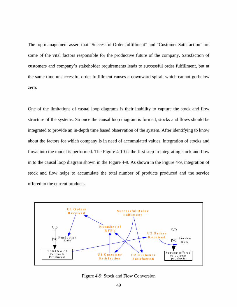
The top management assert that “Successful Order fulfillment” and “Customer Satisfaction” are
some of the vital factors responsible for the productive future of the company. Satisfaction of
customers and company’s stakeholder requirements leads to successful order fulfillment, but at
the same time unsuccessful order fulfillment causes a downward spiral, which cannot go below
zero.
One of the limitations of casual loop diagrams is their inability to capture the stock and flow
structure of the systems. So once the causal loop diagram is formed, stocks and flows should be
integrated to provide an in-depth time based observation of the system. After identifying to know
about the factors for which company is in need of accumulated values, integration of stocks and
flows into the model is performed. The Figure 4-10 is the first step in integrating stock and flow
in to the causal loop diagram shown in the Figure 4-9. As shown in the Figure 4-9, integration of
stock and flow helps to accumulate the total number of products produced and the service
offered to the current products.
U 2 C u s to m e rS a tis fa c t io n
U 2 O rd e rsR e c e iv e d
S u c c e s s fu l O rd e rF u lf ilm e n t
U 1 C u s to m e rS a tis fa c t io n
N u n m b e r o fR F P 's
U 1 O rd e rsR e c e iv e d
T o ta l N o o fP ro d uc ts
P ro d uc e d
P ro d uc tio nR a te
S e rv ic e o ffe re dto c urre ntp ro d uc ts
S e rvic eR a te
Figure 4-9: Stock and Flow Conversion
49

Marketing personnel such as Director of Marketing and Marketing Research Analyst are
interviewed to help in building the market model shown in the Figure 4-11 and 4-12. The market
model gives an idea of how the existing customer base increases through customer conversion.
The existing customers along with good satisfaction level increase the number of satisfied
customers, as the number of satisfied customers increases the number of winning proposals
increases. The increase in the winning proposals indicates that the there is an increase in the
fruitfulness, which is the possible conversion of potential customers in to actual customers. So
the increase in the fruitfulness increases the conversion, which in turn increases the actual
customers.
Satisfied.Customers
Winning Proposals
Customerconversion
CustomersSatisfaction level
Fruitfulness
+
+
+
+
+
Figure 4-10: Market Model
A more sophisticated product/market behavior representation is shown in Figure 4-12 which is
developed to capture the stocks of the market model segment. Word-of-mouth is one of the
50
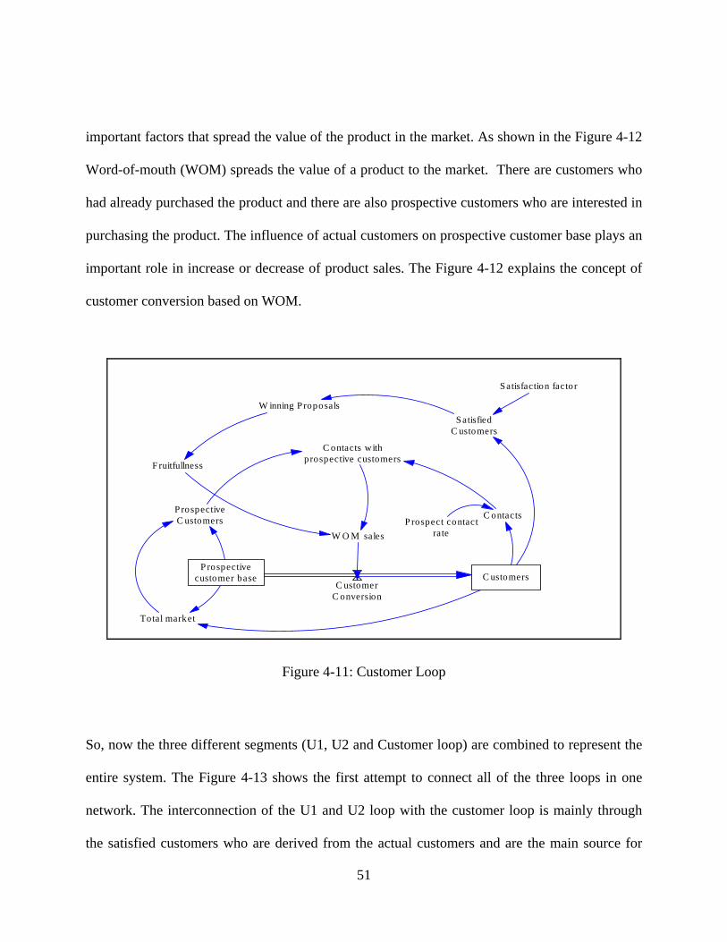
important factors that spread the value of the product in the market. As shown in the Figure 4-12
Word-of-mouth (WOM) spreads the value of a product to the market. There are customers who
had already purchased the product and there are also prospective customers who are interested in
purchasing the product. The influence of actual customers on prospective customer base plays an
important role in increase or decrease of product sales. The Figure 4-12 explains the concept of
customer conversion based on WOM.
P rospectiveC ustomers
C ontacts withprospective customers
P rospect contactrate
Total market
W O M sales
P rospectivecustomer base C ustomers
C ontacts
C ustomerC onversion
F ruitfullness
S atisfiedC ustomers
W inning P roposals
Satisfaction factor
Figure 4-11: Customer Loop
So, now the three different segments (U1, U2 and Customer loop) are combined to represent the
entire system. The Figure 4-13 shows the first attempt to connect all of the three loops in one
network. The interconnection of the U1 and U2 loop with the customer loop is mainly through
the satisfied customers who are derived from the actual customers and are the main source for
51
increasing the number of winning proposal to a higher level. The increase in the Winning
Proposals indicates that more number of products to be produced (U1) and this increase in the
production drives the service process (U2) as shown in the Figure 4-13.
At this point, it is realized that though a comprehensive model is developed, it would still be very
difficult to analyze and debug the model. So after having a series of discussions and interviews
with Customer Service, Product Management, Engineering, Quality Control and all other
personnel, the necessary stocks and flows are added to the model. The conversion of the causal
loops to stock and flows required many iterations and calibrations to obtain the different
differential and auxiliary equations (and its respective parameters – See Figure 4-14).
The model generated more than 40 simultaneous equations (including differential and auxiliary
equations). A simpler version of the entire network with a stock and flow model capturing three
main stocks: U1 products, U2 services, and customers is shown in the Figure 4-14.
52

ProspectiveCustomers
Contacts withProspectiveCustomers
Prospect contactrate
Total Market
WOM sales
Prospectivecustomer base Customers
Contacts
Customer Conversion
Fruitfulness
SatisfiedCustomers
Winning Proposals
U2 CustomerSatisfaction
U2 OrdersReceived
Successful OrderFulfillment
U1 CustomerSatisfaction
U1 OrdersReceived
Total No ofProductsProduced
Production Rate
Service offeredto currentproducts
Service Rate
Number of RFP's
Figure 4-12: Initial Interconnection of Primary Loops
53

Figure 4-13: A More Simplified Model
54

The subsequent model development processes are discussed in detail in the upcoming chapters.
Estimation and selection of parameter values, which is the final step in the formulation process,
will be discussed in the next Chapter five. Chapter five also describes the model shown in the
Figure 4-14 by dividing them in to four main segments. Testing and Policy Analysis, which are
the final two steps of model development process is discussed in the Chapters six and seven.
55
CHAPTER FIVE: MODEL DESCRIPTION
The preceding chapter presents the steps involved in the system dynamics model development.
As a subsequent step, this chapter discusses the different segments of the model. The Section 5.1
elaborates in detail the life cycle of each segment of the model and following that Section 5.2
discusses in detail the estimation and selection of parameter values which is the final step of the
formulation process.
5.1 Model Segmentation
The model consists of the following four main sections:
• U1- Product life cycle;
• U2 - Service life cycle;
• Customer conversion/loss/recovery loop; and
• Customer request for proposals.
5.1.1 U 1 Product Life Cycle
Winning proposals from the customer drives the U1 production process. Whenever a proposal is
won, the U1 produces the required number of products and delivers it to the customers at the
specified time in the manner requested. Once the U1 products are produced and delivered to the
56

customers, the U2 service starts delivering services to these products. There is a period of time
(average product lifetime) after which the products are no longer offered for sale by U1. At the
end of the product lifetime, the products are retired. Therefore, after the product retirement
period, the products that are used in the market are termed as discontinuous products. We came
to know from the Director of Product Management states that for the current model the average
product lifetime is 4 years. The Figure 5-1 represents the U1-Product lifecycle, which is basically
derived from the causal loop/stock and flow diagram shown in Figure 4-7.
Figure 5-1: U1 Product Life Cycle
5.1.2 U 2 Service Life Cycle
U2 service group becomes active once the U1 products are made available to the customers.
Once the products are available, U2 initiates the service process for these products. After
discussing with the Customer Service personnel, it is found that even though the product reaches
57

the end of its lifetime and if it is no longer offered for sale (discontinued product), the service
group still needs to continue to offer services for some period of time for the current products in
the field. This is called service transition, where the service for regular products becomes service
for discontinued products. After a period of time, the services can also be retired. The Figure 5-1
represents the U1-Product lifecycle which was basically derived from the causal loop/stock and
flow diagram shown in Figure 4-7.
Figure 5-2: U 2 Service Life Cycle
After interviewing the Director of Customer Service, the service transition from regular to
discontinuous products takes place after four years (product retirement) and then the service
retires four years from there. In this way, the service is available for a total of eight years
provided that enough spare parts are available. The Figure 5-2 represents the U2-Service
lifecycle which is derived from the causal loop shown in Figure 4-8.
58

5.1.3 Customer Conversion/Loss/Recovery Loop
U 1 and U 2 are assumed to share the same customers. The Market Research Analyst clarified
that there are different types of customers. There are customers who had already purchased the
product (actual customers). There are prospective customers who are interested in purchasing the
product (potential customers). Finally, there are customers who are not satisfied with the product
(disgruntled former customers). It is discovered from the conversation that if U1 is winning
higher requests for proposals from existing customers. These existing customers become more
enthusiastic leading to an increase in the fruitfulness of Word of Mouth (WOM) contacts and a
higher conversion rate. If U1 is winning fewer requests for proposals, it results in lower
fruitfulness and slower conversion rate. Other than WOM conversion, there are conversions of
customers from potential to actual customers, i.e. there are customers who get to know about the
product through some other sources (journal, television, internet and others) other than the
existing customers. This process of conversion is termed as customer accession. Customers may
be unsatisfied with the firm due to issues such as price, competition, technology issues and all
others. Due to ongoing quality levels of products/services and the Successful Orders Fulfilled
(SOF) percentage, customer satisfaction factors for each unit are included in the model. After
series of discussions with the Marketing personnel, the model is set up so that if the firm has
very high quality and delivery rates for both units (U1 and U2), it can slow the rate of customer
becoming disgruntled due to other factors. Customers are recovered by the firm over time
through renewed sales contacts, etc. These recovered customers are then put back into the pool
of potential customers.
59

Figure 5-3 shows both the Customer Loop and Customer Request for proposal portion which is
basically derived from the causal loop shown in the Figure 4-11 .
Figure 5-3: Customer Conversion/Loss/Recovery Loop
60
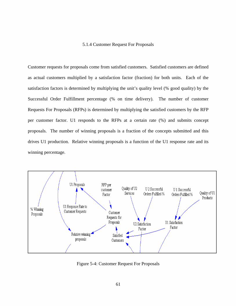
5.1.4 Customer Request For Proposals
Customer requests for proposals come from satisfied customers. Satisfied customers are defined
as actual customers multiplied by a satisfaction factor (fraction) for both units. Each of the
satisfaction factors is determined by multiplying the unit’s quality level (% good quality) by the
Successful Order Fulfillment percentage (% on time delivery). The number of customer
Requests For Proposals (RFPs) is determined by multiplying the satisfied customers by the RFP
per customer factor. U1 responds to the RFPs at a certain rate (%) and submits concept
proposals. The number of winning proposals is a fraction of the concepts submitted and this
drives U1 production. Relative winning proposals is a function of the U1 response rate and its
winning percentage.
Figure 5-4: Customer Request For Proposals
61

The consolidated model shown in Figure 4-13 was developed keeping in mind the importance of
competition, capacity management and other factors The model captures the effect of
competition with help of the market model, the market model manipulates the number of existing
customers, potential customers, and disgruntled customers or in other words customers lost.
Therefore this market model and its variables gives an exact picture of the company’s
performance in the market in comparison to its competitors, because all the manipulations are
done based on the potential market base which is accessible by all the companies. The model
also serves the purpose of the capacity model, that is request for proposal loop gives an idea
about the number of products that the company wins and also the way to improve it with the
increase in some of the important factors (which is described in the Chapter 6). The U1 and U2
model captures all the factors that are considered to be critical in increasing the number of
products per proposal and also the number of services delivered to the customers (described in
the Chapter 6). The cost and financial factors are also considered to be important for the
company’s growth, since it was out of the scope for this research it was included in the future
research.
5.2 Model Variables
This section discusses in detail the several model variables that give a simple representation of
the complex dynamic system. The model has more than 70 variables (Stocks, Rates, Auxiliaries,
and Constants. The variable’s role in the model and their values that are discussed in the
following sections were derived based on the discussions with various personnel from
62
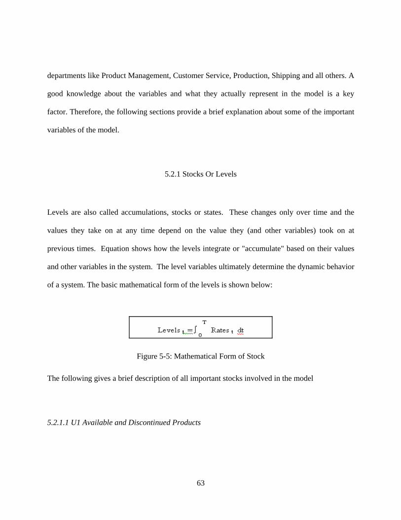
departments like Product Management, Customer Service, Production, Shipping and all others. A
good knowledge about the variables and what they actually represent in the model is a key
factor. Therefore, the following sections provide a brief explanation about some of the important
variables of the model.
5.2.1 Stocks Or Levels
Levels are also called accumulations, stocks or states. These changes only over time and the
values they take on at any time depend on the value they (and other variables) took on at
previous times. Equation shows how the levels integrate or "accumulate" based on their values
and other variables in the system. The level variables ultimately determine the dynamic behavior
of a system. The basic mathematical form of the levels is shown below:
Figure 5-5: Mathematical Form of Stock
The following gives a brief description of all important stocks involved in the model
5.2.1.1 U1 Available and Discontinued Products
63

The growth of new business amplifies as the proposals increases. This increase in the proposal
increases the number of available products in the market. The U1 available products are the total
number of products that are currently used by the customers in the field. After discussing with
the Director of Product Management, there are at least 10 products sent out at the initial stage
that would be used for demos and also for other important purposes. Therefore, we choose the
initial value for the current model to be 10. As already discussed, the current active products
retire after four years and hence discontinued products are the sum of all discontinued products
which are currently eligible for service.
5.2.1.2 Services for Current and Discontinued Products
The service for current products is the sum of all the services performed for the products
currently used in the filed. As already discussed current active products retire after 4 years and
after that they are called discontinued products, but still these discontinued products will have
service for 4 more years. “Services for Discontinued Products” is the sum of all the services
performed for the discontinued products.
5.2.1.3 Potential Customers and Actual Customers
Actual customers increase as potential customers are converted through word of mouth
conversions. After discussions with the Marketing personnel, we set the initial value of Actual
64

customers to be equal to “% of Total Market that are Initial Customers” times the “Total
Market”. Hence the initial value of Potential Customers is (1 - “% of Total Market that are Initial
Customers”) times the “Total Market”.
5.2.2 Rates or Flows
These are the variables that directly change the levels. Rates are essentially the same as
auxiliaries and differ only in the way they are used in a model. These are computed from levels,
constants, and auxiliaries.
Figure 5-6: Mathematical Form of Levels
The following gives a brief description of the rates, which were derived after series of
discussions with various company personnel
1. Production = Average Product per RFP*Winning Proposals/Average Time to
manufacture U1 Products (Products /Month)
65

2. Product Transition = U 1 Available Products/Average Product Lifetime (Products
/Month)
3. Service Development = Services rate over available products*U 1 Available Products
(Services /Month)
4. Service Transition = Service Rate for Discontinued Products*U1 Discontinued Products
(Services / Month)
5. Service Retirement = Services for discontinued products/Time for Service Retirement
Rate (Services /Month)
6. Converting = WOM Conversions + Customer Accession (Customers /Month)
5.2.3 Lookup Tables
In a fair number of places within the model we utilize lookup tables to form a curve that meets a
couple of criteria. The lookup table converts the input (usually a dimensionless ration) to a
output effect or in other words it represents some nonlinear relationships. The variables, a graph,
and some other parameters are discussed in this section.
After series of discussions with the Marketing Research Analyst, it is discovered that there are
certain places in the model where we need to create lookup tables, like (1) the effect of each
unit’s (U1 & U2) satisfaction factor on the fraction of customers at risk (Effect on Fraction of
Customers at Risk due to U1 Customer Satisfaction), (2) the effect of each unit’s (U1 & U2)
satisfaction factor on time to lose customers (Effect on Time to Lose Customers due to U1
66

Customer Satisfaction), and (3) the effect of relative winning proposals on fruitfulness . The
lookup tables and their values, which are explained in this section, are derived based on the
inputs given by the Marketing Research Analyst. It is decided that at customer satisfaction levels
less than 0.70, the fraction at risk would remain at 100%. But if the customer satisfaction levels
are above 70%, the fraction at risk would drop down and at 85% satisfaction, only 60% of the
customers would be at risk. At 80% customer satisfaction, the curve starts to flatten out, and at
100% customer satisfaction, no customers would be at risk.
Figure 5-7: Effect on Fraction of Customers at Risk due to U1 Customer Satisfaction
Similarly, we develop a lookup table for the effect on time to lose customers for each unit (U1 a
be as short as 50% of the normal time or one year. nd U2) customer satisfaction factor which is
shown in the Figure 5-7. At 100% customer satisfaction, we enter a multiplier effect of 3, that is
it takes three times the normal time to lose the customers. At very low satisfaction levels it is
decided that the time to lose a customer could
67

Figure 5-8: Effect on Time to Lose Customers due to U2 Customer Satisfaction
As it can be observed in the Figure 5-7, there is a great risk of losing customers if the satisfaction
factor is low and the risk decreases as the satisfaction factor increases.
5.2.4 Auxiliaries
Auxiliaries are variables computed from Levels, Constants, and other Auxiliaries. They have no
memory, and their current values are independent of the values of variables at previous times.
Figure 5-9: Mathematical Form of Auxiliaries
68

The following gives a brief description of some of the auxiliaries used in the model:
1. Time to manufacture U1 Products;
2. Contacts of non-customers with customers;
3. Customer Request for Proposals;
4. Fruitfulness;
5. Potential Customer Concentration; and
6. Quality of U1 Products.
5.2.5 Other Variables
We are unable to get historical data’s for all the variables. Based on the discussions, it seems
realistic to assume a constant value for some of them but it seems unrealistic for some others. So
minimal data is collected and a distribution is chosen for those variables where assumptions of
constant values seemed unrealistic. After series of discussions, the best values for the constants
are estimated based on their characteristics in such a way to keep up the model at high level of
depiction of reality.
Some of the important constants and their values are
a. Total potential market = 500 customers
b. % of Total potential market that are initial customers = 10%
c. Sociability = 0.1 contacts/customers/Month
d. Average time to produce U1 products= 1 month
69

e. Average product life time = 4 years
f. Average service life time = 8 years
g. Fruitfulness = .3333 people/ contact
5.2.5.1 Fitting Distributions to Variables With Minimal Data
Distributions like Triangular, Exponential, Uniform, Normal are the most reasonable and reliable
distributions when it comes to fitting distribution to variable with minimal or no data [26].
The variables with minimal data are:
h. U1 Response Rate to Customer Requests = 45% to 70% with most likely value of 60%
i. %Winning proposal = 40% to 60% with most likely value of 55%.
j. U1 Successful Orders Fulfilled = 89% to 93% with most likely value of 91%
k. U2 Successful Orders Fulfilled = 87.5% to 91% with most likely value of 89%
Though the above said variables have a minimum and maximum value, it is required to spread
the majority of the data around the most likely value and few around the minimum and
maximum value. Triangular distribution seemed to be the most highly reliable fit for this
scenario, so we choose Triangular distribution for the variables (h-k)
l. Average product per RFP = 1 to 3 products
m. Quality of U1 products = 89.5% to 94%
n. Quality of U2 Services = 87.5% to 92.5%
70

For the above said variables, the values are supposed to be evenly distributed between the
maximum and minimum value and hence uniform distribution, which is the best fit for this
scenario is chosen for the variables (l to n)
5.2.5.2 Fitting Distributions to Historical Data
Historical data of the defect rate (number of defects per month) are available. Kolmogrov-
Smirnov test (K-S) test for goodness-of-fit is conducted for this data, because this test determines
the fit of the possible distributions. Weibull, Lognormal, Exponential and Normal are the best
distributions that fit the defect rate scenario. But based on two main reasons namely (1) the
nature of the problem, which causes the defects, and (2) K-S test results, Weibull distribution is
selected to represent the defect rate.
Lookup tables and constants are chosen to keep up the model at high level of depiction of reality.
By substituting the constants and lookup tables and the distributions the model is able to produce
the expected outputs (production rate, service rate). Please see the Appendix for the rest of the
equations and variables.
71

CHAPTER SIX: MODEL ANALYSIS
“No I ain’t got a witness and I can’t prove it
But that’s my story and I’m sticking to it “
- Lee Roy Parnell and Tony Haselden
What makes a good model? As a modeler, how do you know the results can be trusted? As a
model consumer, when should you accept a model as the basis for action? Once the model is
developed, it is required to make sure that the model depicts the reality and hence it can be used
for policy evaluation. So as soon as the model is developed and the parameter values are chosen,
the model and its behavior are discussed with various team members. This series of discussions
and interviews with the company personnel help to corroborate the validity of the model in
analyzing the current and proposed structure. Following the validity of the model, we perform an
extended analysis, which is the main focus of this chapter. The Section 6.1 explains the various
model testing that is performed to validate the model. The Section 6.2 describes model output
which discusses the output of the model that is illustrated to the company personnel. The Section
6.3 describes sensitivity analysis, which assists in identifying the significant behavior of the
model with respect to the variations in the model parameters.
72
6.1 Model Testing
By definition no model can ever be verified or validated, this is for the reason that all models,
mental or formal, are limited, simplified representations of the real world. “Useful”,
“Convincing” or “Inspiring Confidence” are more apt descriptors applying to model than
“Valid”. So in order to gain confidence on the model, various testing has to be done. Instead of
seeking a single test of validity, modelers should seek multiple point of contact between the
model and reality. According to John D.Sterman [3], a set of standard questions should be
answered satisfactorily in order to gain confidence in a system dynamics model. Those questions
are designed to (1) assess the overall suitability of the model to the purpose, (2) its conformance
to fundamental formulation principles, (3) sensitivity of results to uncertainty in assumptions and
the integrity of the modeling process. Hence, this section explains in detail the answers to those
set of questions in relevance to this thesis, with the help of various tests that was conducted
during and after the model development process.
1) What is the purpose of the model?
In this thesis, the main purpose of creating a system dynamics model is to
investigate the various circumstances that would result in a decline in the growth of the
company. . As a subsequent step it also should assist in choosing the best policy that
would help to sustain the growth of the company.
73

2) What is the boundary of the model? Are the issues important to the purpose treated
endogenously? Are important variables excluded because of no numerical data?
Boundary adequacy tests assess the appropriateness of the model boundary for the
purpose of the model. This test helps to answer whether all the important factors for
addressing the problem are endogenous to the model. Discussions are held with various
teams like Marketing, Customer Support and Quality to make sure that all the important
factors are incorporated in to model. These discussions helped a lot in improving the
model with respect to the boundary adequacy. For example, when the model is first
formulated, the customer part of the model had only the WOM conversion of customers
(shown in Figure 4-12) but after series of discussions with the marketing personnel it was
found that there are also customers who get to know about the product from sources other
than the existing customers, so this concept is introduced in to the model as customer
accession (shown in Figure 4-14). As a subsequent step, it is tested to see how well the
customer loop behaves. It is found from the test that there is an increase in the customer
conversion due to the customer accession factor and this customer loop behavior is more
realistic. So the customer accession is included as an endogenous variable of the model.
So after the entire simplified model is formed, it is presented to the various members and
it is made sure that all the appropriate factors are made endogenous to the model.
74

3) What is the time horizon relevant to the problem? Does the model include the factors that
may change significantly over the time horizon as endogenous elements?
After series of discussions with the decision makers, the time horizon for the
model is set to 5 years in such a way to capture the delayed and indirect potential policies
of the company. Further the parameters that change significantly over the time horizon
such as customers, winning proposals, production, service and others are incorporated in
to the model as endogenous elements.
4) Is the level of aggregation consistent with the purpose?
Yes. The model has the level of aggregation to answer the questions
relevant to the growth of the company and the corporate policies required for this. In
addition, using the reference modes, the model is able to check for the fear and hope of
the company. This provides confidence with the aggregation level.
5) Does the model confirm to basic physical law such as conservation of matter? Is the stock
and flow structure explicit and consistent with the model?
Structure assessment test investigates whether the model is consistent with the
knowledge of the real system relevant to the purpose. It focuses on the conformance of
the model to the physical realities such as realism of the decision rules and conservation
75

law. Hence the model is tested for inappropriate assumptions, inconsistence and all other
factors that obliterate the model conformance to the reality. For example there are stocks
such as number of products currently used in the market and service for products, which
cannot turn out to be a negative value. Hence series of analysis are conducted and it is
made sure that the stocks do not become negative at any instance of the simulation
process. So, these tests further helped in corroborating the validity of the model.
6) Are all the equations consistent dimensionally with out the use of fudge factors?
Dimensional consistency is one of the basic tests that should be done at the initial
stage. This test helps in identifying the important flaws in the understanding of the
structure or the decision process that are being modeled. Hence the dimensional check is
performed using the command “Unit check” in Vensim. The test confirms that all the
variables in the model are defined with the correct unit of measure.
7) Are people assumed to act rationally and to optimize their performance? Does the model
account for cognitive limitations, organizational realities, non-economic motives and
political factors?
Yes. This is verified. The organization realities, the separation of the business and
non-economic motives such as socialization are taken into consideration.
76

8) Are the simulated decisions based on information the real decision makers actually have?
Are appropriate time delays, constraints, and possible bottlenecks taken into account?
The interviews and group discussions conducted with the different teams of the
company helped in gathering all the important information for the model. Hence all the
information used in this model are based on the information that the real decision makers
had. The appropriate time delays and constraints were incorporated in to the model with
the help of various factors such as product retirement time, service retirement time, time
to lose customers, fruitfulness and others. For example, the customer satisfaction is a
factor that determines the customer loss, meaning if the customer satisfaction is high then
the customer loss is low but if the customer satisfaction is low then the customer loss
high. Designing a look up table with customer satisfaction as the input, effectively
captured the above-mentioned customer loss characteristic.
9) Is the model robust in the face of extreme variations in input conditions or policies?
The model is subjected to large shocks and extreme conditions and is then
examined to see if its response is reasonable under these uncertainties. For example, the
model is simulated under extreme conditions and is made sure that the potential
customers neither increases above the total potential market nor decreases below zero.
Sensitivity analysis technique that supports this test is explained in detail in the following
Section 6.3.
77

10) Are the policy recommendations sensitive to the plausible variations in the assumptions,
including assumptions about the parameters, aggregation, and model boundary?
The policy recommendations are established based on the behavioral changes in
the model output, when certain parameters are changed over a plausible range of values,
which are based on the discussions with the various team members. Hence these policies
are meant to assist the company to continue in the path of success even when it is hit by
uncertainties.
11) What types of data are used to develop and test the model?
Historical data are not available for all the parameters, but based on the
discussions it seemed realistic to assume a constant value for some of them but it seemed
unrealistic for some. So minimal data are collected and a distribution is chosen for those
variables where assumptions of constant values seemed unrealistic. After series of
discussions the best values for the constants and the distributions were defined based on
their characteristics in such a way to keep up the model at high level of depiction of
reality.
78
12) How do modelers describe the process they used to test and build confidence in the
model? Did critics and independent third parties review the model?
Demonstration of the model segments to the relevant teams at the appropriate
time of model development helped in building confidence in the model. For example,
when the customer segment of the model was developed various discussions were held
with the Marketing personnel and their feedbacks and questions are gathered. These
feedbacks and questions are exceptional factors that assist in improving the model’s
conformance to reality. Further, parameter assessment test help in validating the model
by confirming that all the model variables have a clear meaning. Discussions that are held
during the model development process, helped to identify those variables that do not fit
the real life meaning. Hence, further research is conducted and data pertaining to the
variable are collected. For example, at the initial stage of the modeling process, the
number of defects is calculated at a constant rate, meaning it is assumed that the defect
rate is 2% throughout the simulation process. But interviews with the Customer Service
personnel reveal that the number defects per month are not constant and hence assuming
a constant to that variable compromises the model conformance to reality. Hence,
historical data are collected and statistically analyzed. Once the entire model is
developed, it is illustrated to all the team members, which further corroborated the
model’s validity.
13) Are the results of the model reproducible? Are the results add-forced by the modeler?
79

Random distributions such as Uniform, Weibull and others are used in the model.
Due to the randomness created by these distributions, the model is simulated for various
replications. The number of replications is set to 16. After 16 replications, the average of
the output is determined, which is used to represent result of all the replications.
14) How long does it take to revise and update the model?
The teams are consulted independently during the initial stages of the model
development to form the different segments of the model. Once all the individual
segments of the model are formed, they are all connected to form one simple realistic
model. The entire model is then explained to all the teams that helped in gathering
feedback from the team members. As a subsequent, step the model is revised and updated
based on the feedback, which took nearly two to three weeks.
15) What are the biases, ideologies and political agendas of the modelers and clients? How
might these biases affect the results?
Assumptions:
80

a) In this model it is assumed that management will invest in new product
developments and other proposals only if the marginal rate of return exceeds the
marginal rate of cost. As a result, profit and loss variables are not included.
However, not all products and proposals will be successful but the gainers must
exceed the losers.
b) In this model, it is assumed that there is no negative word of mouth
between disgruntled former customers and potential customers.
c) In this model, it is assumed that the total number of products produced is
used by the customers through out the product and service life time.
d) After series of discussions, variables such as total potential market,
sociability, are assumed to be constant. These constants are chosen to keep up the
model at high level of depiction of reality.
81

6.2 Model Output And Discussions
As already seen in the earlier chapters, the model is developed based on the information
collected from different team members. The model is then validated and made sure that it is the
expected real world representation of the system under study. As a subsequent step the model
was simulated and the results were shown to the decision makers (Director of Product
Development, Director of Customer Service, and others). But the model had nearly eight random
distributions. Since the randomness of the distributions might affect the simulation results and
also in order to keep up the proximity to reality, it is decided to strengthen the results by running
the model simulation for 30 replications. Therefore, the model is replicated 30 times and the
average of output values (such as number of available products, actual customers, services and
others) for the 30 replications is computed and shown to the decision makers. To make sure that
this approach of representing the set of 30 outputs with the average value is reasonable, the
standard deviation of output values is calculated and analyzed and is made sure that there is not
much of variation in the output values for 30 replications.
6.2.1 Model Output
The following section of graphs shows the important output values for different replications of
the model and also the average output values of all replications (hope of the company) versus the
fear of the company that might come up due to influence of the inflection point.
82

U 1 Available Products2,000
1,500
1,000
500
00 3 6 9 12 15 18 21 24 27 30 33 36 39 42 45 48 51 54 57 60
Time (Month)
U 1 Available Products : Replication 16 productsU 1 Available Products : Replication 15 productsU 1 Available Products : Replication 14 productsU 1 Available Products : Replication 13 productsU 1 Available Products : Replication 12 productsU 1 Available Products : Replication 11 productsU 1 Available Products : Replication 10 productsU 1 Available Products : Replication 9 productsU 1 Available Products : Replication 8 productsU 1 Available Products : Replication 7 productsU 1 Available Products : Replication 6 productsU 1 Available Products : Replication 5 productsU 1 Available Products : Replication 4 productsU 1 Available Products : Replication 3 productsU 1 Available Products : Replication 2 productsU 1 Available Products : Replication 1 products
Figure 6-1: Available Products
It is observed from the Figure 6-1 that the number of active or continuous products available in
the field accumulates to around 1500 over a period of 60 months, indicating that the product
performance in the market is improving. This performance is then projected against threat of
inflection point with the help of fear curve.
83

Actual Customers200
150
100
50
00 3 6 9 12 15 18 21 24 27 30 33 36 39 42 45 48 51 54 57 60
Time (Month)
Actual Customers : Replication 16 customersActual Customers : Replication 15 customersActual Customers : Replication 14 customersActual Customers : Replication 13 customersActual Customers : Replication 12 customersActual Customers : Replication 11 customersActual Customers : Replication 10 customersActual Customers : Replication 9 customersActual Customers : Replication 8 customersActual Customers : Replication 7 customersActual Customers : Replication 6 customersActual Customers : Replication 5 customersActual Customers : Replication 4 customersActual Customers : Replication 3 customersActual Customers : Replication 2 customersActual Customers : Replication 1 customers
Figure 6-2: Actual Customers
The graph in Figure 6-2 shows that the number of actual customers increases to 150 over a
period of 60 months, this behavior is because of the fact that there is a considerable measure of
customer conversion from potential to actual customers due to the improved product
performance. Further, this increase in the actual customers is also projected against the threat of
the inflection point with the help of fear curve.
84
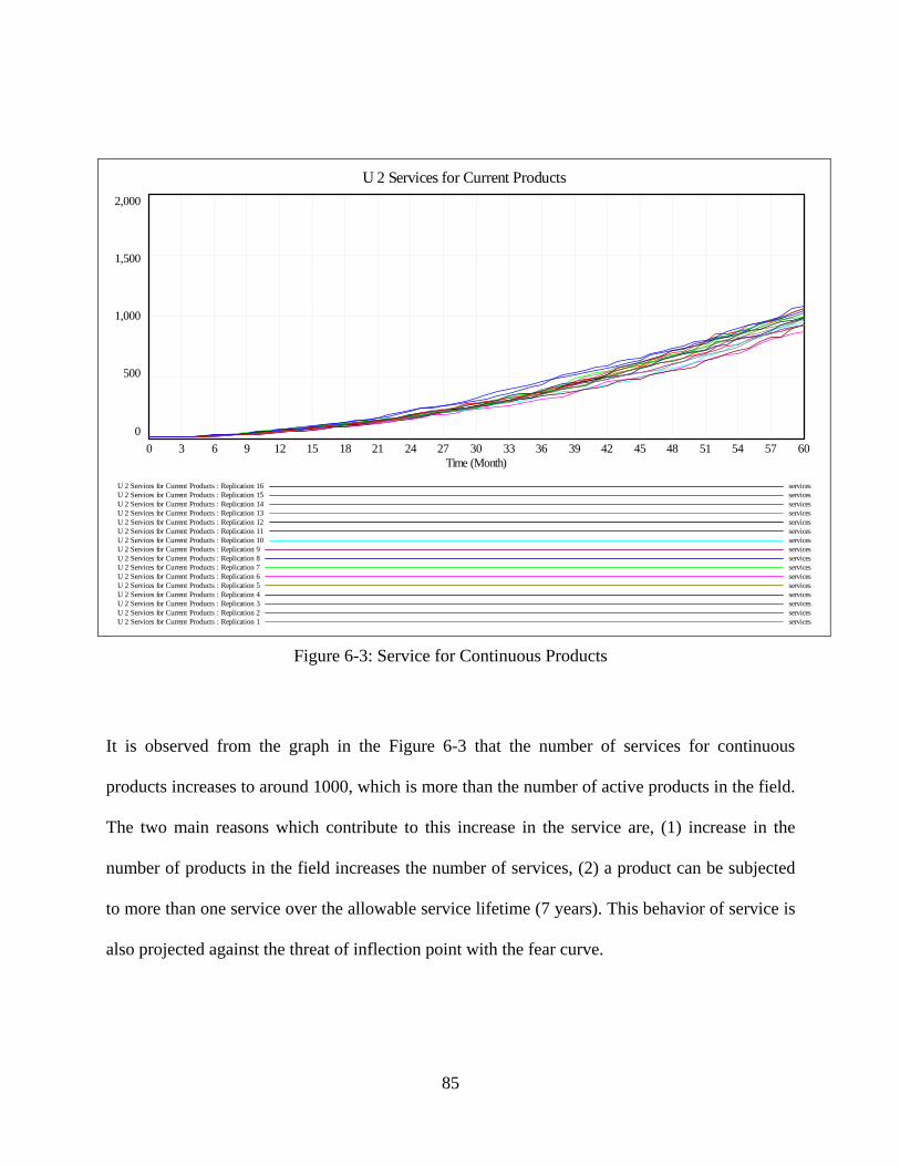
U 2 Services for Current Products2,000
1,500
1,000
500
00 3 6 9 12 15 18 21 24 27 30 33 36 39 42 45 48 51 54 57 60
Time (Month)
U 2 Services for Current Products : Replication 16 servicesU 2 Services for Current Products : Replication 15 servicesU 2 Services for Current Products : Replication 14 servicesU 2 Services for Current Products : Replication 13 servicesU 2 Services for Current Products : Replication 12 servicesU 2 Services for Current Products : Replication 11 servicesU 2 Services for Current Products : Replication 10 servicesU 2 Services for Current Products : Replication 9 servicesU 2 Services for Current Products : Replication 8 servicesU 2 Services for Current Products : Replication 7 servicesU 2 Services for Current Products : Replication 6 servicesU 2 Services for Current Products : Replication 5 servicesU 2 Services for Current Products : Replication 4 servicesU 2 Services for Current Products : Replication 3 servicesU 2 Services for Current Products : Replication 2 servicesU 2 Services for Current Products : Replication 1 services
Figure 6-3: Service for Continuous Products
It is observed from the graph in the Figure 6-3 that the number of services for continuous
products increases to around 1000, which is more than the number of active products in the field.
The two main reasons which contribute to this increase in the service are, (1) increase in the
number of products in the field increases the number of services, (2) a product can be subjected
to more than one service over the allowable service lifetime (7 years). This behavior of service is
also projected against the threat of inflection point with the fear curve.
85
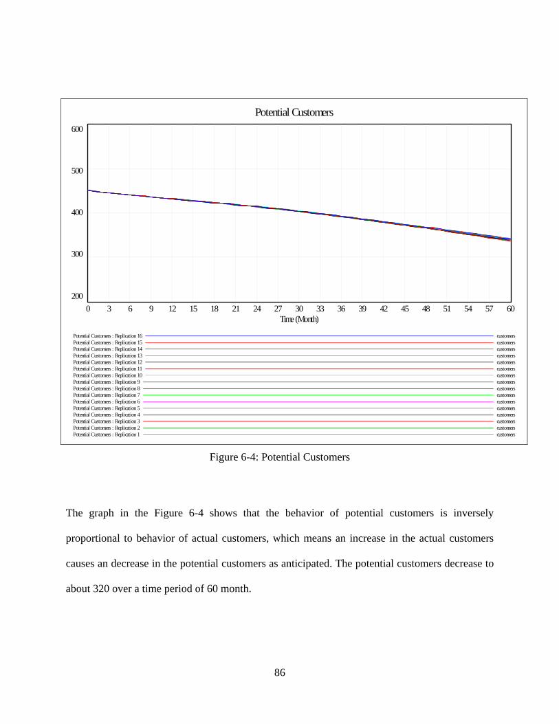
Potential Customers600
500
400
300
2000 3 6 9 12 15 18 21 24 27 30 33 36 39 42 45 48 51 54 57 60
Time (Month)
Potential Customers : Replication 16 customersPotential Customers : Replication 15 customersPotential Customers : Replication 14 customersPotential Customers : Replication 13 customersPotential Customers : Replication 12 customersPotential Customers : Replication 11 customersPotential Customers : Replication 10 customersPotential Customers : Replication 9 customersPotential Customers : Replication 8 customersPotential Customers : Replication 7 customersPotential Customers : Replication 6 customersPotential Customers : Replication 5 customersPotential Customers : Replication 4 customersPotential Customers : Replication 3 customersPotential Customers : Replication 2 customersPotential Customers : Replication 1 customers
Figure 6-4: Potential Customers
The graph in the Figure 6-4 shows that the behavior of potential customers is inversely
proportional to behavior of actual customers, which means an increase in the actual customers
causes an decrease in the potential customers as anticipated. The potential customers decrease to
about 320 over a time period of 60 month.
86

U2 service for Discontinued Products200
165
130
95
600 3 6 9 12 15 18 21 24 27 30 33 36 39 42 45 48 51 54 57 60
Time (Month)
U2 service for Discontinued Products : Replication 16 servicesU2 service for Discontinued Products : Replication 15 servicesU2 service for Discontinued Products : Replication 14 servicesU2 service for Discontinued Products : Replication 13 servicesU2 service for Discontinued Products : Replication 12 servicesU2 service for Discontinued Products : Replication 11 servicesU2 service for Discontinued Products : Replication 10 servicesU2 service for Discontinued Products : Replication 9 servicesU2 service for Discontinued Products : Replication 8 servicesU2 service for Discontinued Products : Replication 7 servicesU2 service for Discontinued Products : Replication 6 servicesU2 service for Discontinued Products : Replication 5 servicesU2 service for Discontinued Products : Replication 4 servicesU2 service for Discontinued Products : Replication 3 servicesU2 service for Discontinued Products : Replication 2 servicesU2 service for Discontinued Products : Replication 1 services
Figure 6-5: Service for Discontinuous Products
The graph in the Figure 6-5 shows that the service for discontinuous products also increases with
time but this increase is less compared to the number of services for continuous products. The
main reason that contribute to this variation in the number of services is the average product
lifetime, since the average product lifetime is 4 years there is a delay in the transition of the
services and hence the number of services for continuous products is always greater than the
service for discontinuous products
87

6.2.2 Conclusion
It was observed from the graphs that the performance of the company in the market is improving
with respect to product, service and customers. This behavior as explained in the above section
and many others were reported to different team members of the company. However the fear
curve was an intimidating feature of the above shown graphs, though the decision makers were
happy with the performance of the company for the current effort, they were very keen in
identifying the factors that would transform the course of the current path towards the path of
fear curve. The sensitivity analysis, which is explained in the next section, helped in identifying
the factors that caused a decline in the growth of the company.
88

6.3 Model Analysis
Model analysis is a tool to determine how “sensitive” a model is to changes in the value of
parameters of the model and to changes in the structure of the model. In this thesis we mainly
focus on parameter sensitivity in view of the fact that it helps to identify the parameters and
relationships to which the behavior and policy recommendations are sensitive. Parameter
sensitivity is usually performed as a series of tests in which we set different parameter values to
see how a change in the parameter causes a change in the dynamic behavior of the stocks.
After series of conversations with the various company personnel the most important parameters
and the response variables that were hypothesized to be critical for the performance of the
company were identified. In the following section we will discuss those parameters and the
dynamic behavior of the model with respect to the change in the parameters.
The response variables that are going to be analyzed are: (1) U1- products or the number of
products produced (2) U2 service or the number of services to be preformed and (3) number of
actual customers. In the following sections the parameters (for example time for production,
quality of product and others) are varied over a limit and the corresponding variation in the
response variables are discussed. Some of the parameters has distribution as their input, but for
the purpose of sensitivity analysis those distributions were replaced by the most likely value of
the parameter.
89

6.3.1 Model Analysis And Sensitivity To Changes In The Parameters
For the present operating conditions of the company; the graphs in the Figure 6-6 shows the
behavior that would be exhibited by products, services, and customers over a time. The
following sections would explain how a change in some of the model parameters causes a
change in these behaviors.
Available Products
0200400600800
1000120014001600
1 6 11 16 21 26 31 36 41 46 51 56
Time
Prod
ucts
Services for Current Products
0
200
400
600
800
1000
1200
1 6 11 16 21 26 31 36 41 46 51 56
Time
Serv
ices
Customers
0
100
200
300
400
500
1 4 7 10 13 16 19 22 25 28 31 34 37 40 43 46 49 52 55 58
Time
Cus
tom
ers
Actual Cust Potential Cust
Figure 6-6: Initial behavior of Product, Service & Customers
90

6.3.1.1 Quality of U2 services
The quality of U2 services has severe effect on customers, U1 products and U2 services. The
graphs in the figure 6-7 show all plots (from 25% to 100% of U2 service quality). The highest
quality causes an increase in U1 products and U2 services and customers as expected. However
the plot for 25 % and 50% quality is barely visible at the bottom of the axis and the plot for 75%
indicates that though there is an increase in the response variables, but the magnitude of increase
is very less and hence the company can not survive with such quality of service.
U 1 Available Products2,000
1,500
1,000
500
00 6 12 18 24 30 36 42 48 54 60
Time (Month)
U 1 Available Products : Qual U2 95 productsU 1 Available Products : Qual U2 75 productsU 1 Available Products : Qual U2 50 productsU 1 Available Products : Qual U2 25 products
U 2 Services for Current Products2,000
1,500
1,000
500
00 6 12 18 24 30 36 42 48 54 60
Time (Month)
U 2 Services for Current Products : Qual U2 95 servicesU 2 Services for Current Products : Qual U2 75 servicesU 2 Services for Current Products : Qual U2 50 servicesU 2 Services for Current Products : Qual U2 25 services
A c t u a l C u s t o m e r s2 0 0
1 5 0
1 0 0
5 0
00 6 1 2 1 8 2 4 3 0 3 6 4 2 4 8 5 4 6 0
T im e ( M o n th )
A c t u a l C u s t o m e r s : Q u a l U 2 9 5 c u s t o m e rsA c t u a l C u s t o m e r s : Q u a l U 2 7 5 c u s t o m e rsA c t u a l C u s t o m e r s : Q u a l U 2 5 0 c u s t o m e rsA c t u a l C u s t o m e r s : Q u a l U 2 2 5 c u s t o m e rs
Figure 6-7: Effect of U2 Service Quality
91

6.3.1.2 Time To Retire Service
There is no effect on the U1 stock and minor effects on the U2 stock for discontinuous products.
This is because all of the values for retiring services are greater than or equal to the product
lifetime of four years. Thus the service to product ratio will always be at or better than what
customer expect and there is no change in production. The U2 services for discontinuous
products increases due to the increase in the time to retire service, this is because the services for
discontinuous products retire only after the service retirement period and hence increase in the
service retirement accumulates the number of service for discontinuous products. But this
increase is not too high because the number of products sent for services after the product life
time is considerably less.
U 1 Available Products2,000
1,500
1,000
500
00 6 12 18 24 30 36 42 48 54 60
Time (Month)
U 1 Available Products : Time to Retire Service 8 yrs productsU 1 Available Products : Time to Retire Service 6 yr productsU 1 Available Products : Time to Retire Service 4 yrs products
U2 service for Discontinued Products200
150
100
50
00 6 12 18 24 30 36 42 48 54 60
Time (Month)
U2 service for Discontinued Products : Time to Retire Service 8 yrs servicesU2 service for Discontinued Products : Time to Retire Service 6 yr servicesU2 service for Discontinued Products : Time to Retire Service 4 yrs services
Figure 6-8: Effect of Time to Retire Service
92

6.3.1.3 Fruitfulness
Increasing the fruitfulness increases the number of available products and services and the
opposite happens when the fruitfulness is reduced. When the fruitfulness is 65% there is a
considerable number of customer conversion and hence the number products to be produced
increases at a faster rate, but when the fruitfulness reduces to about 10% there is no considerable
number of customer conversion and hence the number request for proposals decreases which
results in lower number of products and services.
U 1 Available Products4,000
3,000
2,000
1,000
00 6 12 18 24 30 36 42 48 54 60
Time (Month)
U 1 Available Products : Fruitfulness 65 productsU 1 Available Products : Fruitfulness 30 productsU 1 Available Products : Fruitfulness 10 products
U 2 Services for Current Products2,000
1,500
1,000
500
00 6 12 18 24 30 36 42 48 54 60
Time (Month)
U 2 Services for Current Products : Fruitfulness 65 servicesU 2 Services for Current Products : Fruitfulness 30 servicesU 2 Services for Current Products : Fruitfulness 10 services
Figure 6-9: Effect of Fruitfulness
93
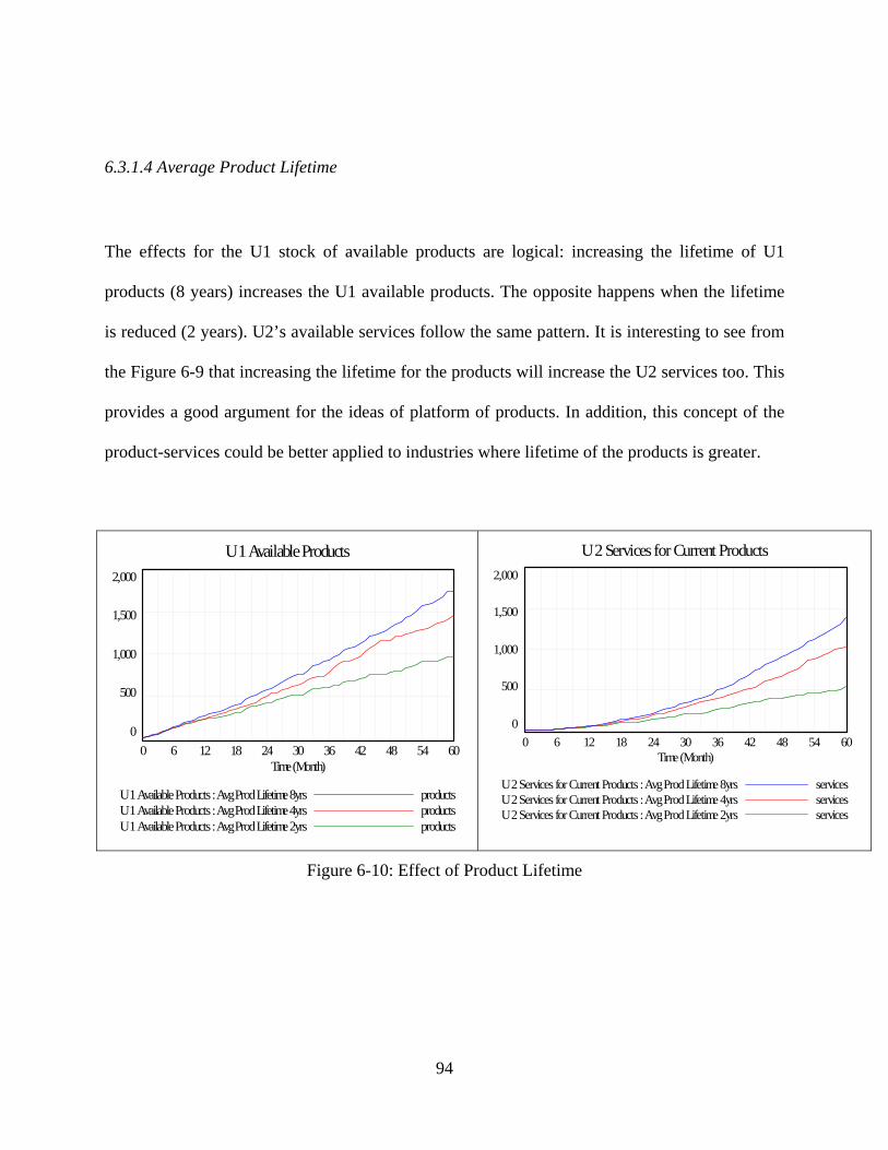
6.3.1.4 Average Product Lifetime
The effects for the U1 stock of available products are logical: increasing the lifetime of U1
products (8 years) increases the U1 available products. The opposite happens when the lifetime
is reduced (2 years). U2’s available services follow the same pattern. It is interesting to see from
the Figure 6-9 that increasing the lifetime for the products will increase the U2 services too. This
provides a good argument for the ideas of platform of products. In addition, this concept of the
product-services could be better applied to industries where lifetime of the products is greater.
U 1 Available Products2,000
1,500
1,000
500
00 6 12 18 24 30 36 42 48 54 60
Time (Month)
U 1 Available Products : Avg Prod Lifetime 8yrs productsU 1 Available Products : Avg Prod Lifetime 4yrs productsU 1 Available Products : Avg Prod Lifetime 2yrs products
U 2 Services for Current Products2,000
1,500
1,000
500
00 6 12 18 24 30 36 42 48 54 60
Time (Month)
U 2 Services for Current Products : Avg Prod Lifetime 8yrs servicesU 2 Services for Current Products : Avg Prod Lifetime 4yrs servicesU 2 Services for Current Products : Avg Prod Lifetime 2yrs services
Figure 6-10: Effect of Product Lifetime
94

6.3.1.5 Successful Order Fulfilled Of U1 Products
Increasing the % of Successful Order Fulfilled increases U1 products. U2’s services follow the
same pattern found for U1. Reducing this variable decreases the rate of growth of available
products and services (but not proportionally!). As shown in the graph, when the order
fulfillment is high there is a considerable increase in the number of customers, products and
services which is due to the customer satisfaction created by the on time delivery. But when the
order fulfillment is as low as 50% there is a severe negative impact and hence the actual
customers diminishes and it is barely visible bottom of the axis and owing to this decreased
customers the number of products also diminishes as shown in the Figure 6-10.
U 1 Available Products
4,000
3,000
2,000
1,000
00 6 12 18 24 30 36 42 48 54 60
Time (Month)
U 1 Available Products : U1 Order Fulfill 100 productsU 1 Available Products : U1 Order Fulfill 90 productsU 1 Available Products : U1 Order Fulfill 75 productsU 1 Available Products : U1 Order Fulfill 50 productsU 1 Available Products : U1 Order Fulfill 25 products
Actual Customers
400
300
200
100
00 6 12 18 24 30 36 42 48 54 60
Time (Month)
Actual Customers : U1 Order Fulfill 100 customersActual Customers : U1 Order Fulfill 90 customersActual Customers : U1 Order Fulfill 75 customersActual Customers : U1 Order Fulfill 50 customersActual Customers : U1 Order Fulfill 25 customers
Figure 6-11: Effect of Order Fulfillment of Products
95

6.3.1.6 Winning Proposal
Increase in the % Winning proposal increases the available products. The graph in the Figure 6-
11 shows that when the % winning proposal increases (75%), the number customers increases,
but when the % winning proposal is as low as 10% the number of customers gained over time
increases to only 100, indicating that when the % winning proposal is low the customers belief
on the product decreases and hence the customer conversion decreases. This decreased customer
conversion results in lower number products.
U 1 Available Products4,000
3,000
2,000
1,000
00 6 12 18 24 30 36 42 48 54 60
Time (Month)
U 1 Available Products : % Win Prop 75 productsU 1 Available Products : % Win Prop 50 productsU 1 Available Products : % Win Prop 25 productsU 1 Available Products : % Win Prop 10 products
U 2 Services for Current Products2,000
1,500
1,000
500
00 6 12 18 24 30 36 42 48 54 60
Time (Month)
U 2 Services for Current Products : % Win Prop 75 servicesU 2 Services for Current Products : % Win Prop 50 servicesU 2 Services for Current Products : % Win Prop 25 servicesU 2 Services for Current Products : % Win Prop 10 services
A ctu al C u sto m ers2 0 0
1 5 0
1 0 0
5 0
00 6 1 2 1 8 2 4 3 0 3 6 4 2 4 8 5 4 6 0
Time (M o nth)
A c tu a l C u s to me rs : % W in P ro p 75 c u s to me rsA c tu a l C u s to me rs : % W in P ro p 50 c u s to me rsA c tu a l C u s to me rs : % W in P ro p 25 c u s to me rsA c tu a l C u s to me rs : % W in P ro p 10 c u s to me rs
Figure 6-12: Effect of % Winning Proposals
96

When the % winning proposal increases to 75%, there is a increase in the number of customers
and this results in the pronounced increase in the number of U1 products and U2 services.
6.3.1.7 Sociability
Increasing the sociability increases the U1 available products. The opposite happens when the
sociability is decreased. It has a very positive impact on U1. U2’s available services follow the
same pattern found for U1. When the sociability is increased to .2, that is when there is a good
contact of the actual customers with the potential customer base there is a good conversion rate
of potential customers which results in increased number of U1 products and U2 services, but at
the same time when the sociability is decreased the conversion of potential customers hardly
takes place and hence there is no increase in the products and services.
U 1 Available Products4,000
3,000
2,000
1,000
00 6 12 18 24 30 36 42 48 54 60
Time (Month)
U 1 Available Products : Soc 20 productsU 1 Available Products : Soc 10 productsU 1 Available Products : Soc 5 productsU 1 Available Products : Soc 2 products
U 2 Services for Current Products2,000
1,500
1,000
500
00 6 12 18 24 30 36 42 48 54 60
Time (Month)
U 2 Services for Current Products : Soc 20 servicesU 2 Services for Current Products : Soc 10 servicesU 2 Services for Current Products : Soc 5 servicesU 2 Services for Current Products : Soc 2 services
Figure 6-13: Effect of Sociability
97

6.3.1.8 Product Per Request For Proposal
Increasing the Product per RFP increases the U1 available products. The opposite happens when
the value is reduced to 1 Product/RFP. U2’s available services follow the same pattern. As
anticipated, the effect of product per RFP causes a proportional change in the number of products
and services as is shown in the Figure 6-13. But this change has no effect on the customers, the
number of customer’s remains the same regardless of the change in the products per RFP.
U 1 Available Products4,000
3,000
2,000
1,000
00 6 12 18 24 30 36 42 48 54 60
Time (Month)
U 1 Available Products : Avg Prd per Prop 4 productsU 1 Available Products : Avg Prd per Prop 2 productsU 1 Available Products : Avg Prd per Prop 1 products
U 2 Services for Current Products2,000
1,500
1,000
500
00 6 12 18 24 30 36 42 48 54 60
Time (Month)
U 2 Services for Current Products : Avg Prd per Prop 4 servicesU 2 Services for Current Products : Avg Prd per Prop 2 servicesU 2 Services for Current Products : Avg Prd per Prop 1 services
A ctu a l C u sto m ers2 0 0
1 5 0
1 0 0
5 0
00 6 1 2 1 8 2 4 3 0 3 6 4 2 4 8 5 4 6 0
Time (M o nth)
A c tua l C usto me rs : A vg P rd p e r P ro p 4 c usto me rsA c tua l C usto me rs : A vg P rd p e r P ro p 2 c usto me rsA c tua l C usto me rs : A vg P rd p e r P ro p 1 c usto me rs
Figure 6-14: Effect of Product per RFP
98

6.3.1.9 Quality of U1 Products
The highest quality of U1 products results in the increase of customers, products and services as
expected. But at a quality level of 25% and 50%, the company looses customers and also it
doesn’t win any products U2’s available services follow the same pattern found for U1. This
behavior is similar to the effect of U2 service quality, but the most important inference from the
Figure 6-15 is that though the company’s growth declines, rate at which it declines is faster when
compared to the effect of U2’s quality.
U 1 Available Products4,000
3,000
2,000
1,000
00 6 12 18 24 30 36 42 48 54 60
Time (Month)
U 1 Available Products : Qual U1 100 productsU 1 Available Products : Qual U1 95 productsU 1 Available Products : Qual U1 75 productsU 1 Available Products : Qual U1 50 productsU 1 Available Products : Qual U1 25 products
U 2 Services for Current Products2,000
1,500
1,000
500
00 6 12 18 24 30 36 42 48 54 60
Time (Month)
U 2 Services for Current Products : Qual U1 100 servicesU 2 Services for Current Products : Qual U1 95 servicesU 2 Services for Current Products : Qual U1 75 servicesU 2 Services for Current Products : Qual U1 50 servicesU 2 Services for Current Products : Qual U1 25 services
Actu al C u sto m ers400
300
200
100
00 6 12 18 24 30 36 42 48 54 60
Time (M onth)
A ctu a l Cu s to mers : Qu a l U1 100 cu s to mersA ctu a l Cu s to mers : Qu a l U1 95 cu s to mersA ctu a l Cu s to mers : Qu a l U1 75 cu s to mersA ctu a l Cu s to mers : Qu a l U1 50 cu s to mersA ctu a l Cu s to mers : Qu a l U1 25 cu s to mers
Figure 6-16: Effect of Quality of U1 Product
99

6.3.1.10 Response Rate to Customer Request
Increased % response rate increases the available products. But the plot for 10% is barely visible
at the bottom, indicating that the decreased % response rate has severe effect on the U1 products,
which measures that if the company’s response to customer request is low then it would have
negative impact on the company. U2’s available services follow the same pattern. The graphs in
the Figure 6-16 shows the behavior of product and services with respect to the change in
response rate. This variable has a similar effect to % winning proposal.
U 1 Available Products2,000
1,500
1,000
500
00 6 12 18 24 30 36 42 48 54 60
Time (Month)
U 1 Available Products : % Resp Rate 75 productsU 1 Available Products : % Resp Rate 50 productsU 1 Available Products : % Resp Rate 25 productsU 1 Available Products : % Resp Rate 10 products
U 2 Services for Current Products2,000
1,500
1,000
500
00 6 12 18 24 30 36 42 48 54 60
Time (Month)
U 2 Services for Current Products : % Resp Rate 75 servicesU 2 Services for Current Products : % Resp Rate 50 servicesU 2 Services for Current Products : % Resp Rate 25 servicesU 2 Services for Current Products : % Resp Rate 10 services
Figure 6-17: Effect of Response Rate to Customer Request
100

6.3.1.11 Time for Production
The graph in the figure indicates that change in the number of products and services are inversely
proportional to the change in the production time. The Figure 6-17 indicates that increasing the
time for production to 2 months halved the number of U1 products and U2 services. But when
the time for production is halved (half month) the number of products and services are doubled.
So it is observed that the growth rate can be tailored with changes in the time for production.
U 1 Available Products4,000
3,000
2,000
1,000
00 6 12 18 24 30 36 42 48 54 60
Time (Month)
U 1 Available Products : Time to Develop Prod 2 month productsU 1 Available Products : Time to Develop Prod 1 month productsU 1 Available Products : Time to Develop Prod half month products
U 2 Services for Current Products2,000
1,500
1,000
500
00 6 12 18 24 30 36 42 48 54 60
Time (Month)
U 2 Services for Current Products : Time to Develop Prod 2 month servicesU 2 Services for Current Products : Time to Develop Prod 1 month servicesU 2 Services for Current Products : Time to Develop Prod half month services
Figure 6-18: Effect of Production Time
101

6.3.1.12 Successful Order Fulfilled Of U2 Service
% of Successful Order Fulfilled of U2 services has severe effect on the U1 products. U2’s
services follow the same pattern found for U1. When the service order fulfillment is reduced it
decreases the rate of growth of available products and services (but not proportionally!). As
shown in the Figure 6-18, when the order fulfillment of U2 is high there is a considerable
increase in the number of customers, products and services. But when the order fulfillment is as
low as 50% there is a severe negative impact and hence the actual customers diminishes and it is
barely visible bottom of the axis and owing to this decreased customers the number of products
also diminishes as shown in the Figure 6-18.
Actual Customers400
300
200
100
00 6 12 18 24 30 36 42 48 54 60
Time (Month)
Actual Customers : Order FulFil U2 100 customersActual Customers : Order FulFil U2 90 customersActual Customers : Order FulFil U2 75 customersActual Customers : Order FulFil U2 50 customersActual Customers : Order FulFil U2 25 customers
U 2 Services for Current Products2,000
1,500
1,000
500
00 6 12 18 24 30 36 42 48 54 60
Time (Month)
U 2 Services for Current Products : Order FulFil U2 100 servicesU 2 Services for Current Products : Order FulFil U2 90 servicesU 2 Services for Current Products : Order FulFil U2 75 servicesU 2 Services for Current Products : Order FulFil U2 50 servicesU 2 Services for Current Products : Order FulFil U2 25 services
Figure 6-19: Effect of Order Fulfillment of Services
102

6.3.2 Summary
As seen in the model analyses there are certain factors which have the capability to cause a
downward spiral in the company’s status. The following are the inferences that were obtained
from the model analysis.
Growth or decline can be easily triggered by changes to several variables such as
Order win rate percentage for U1
Response rate to customer requests for proposals
Quality performance of either U1 or U2
Successful order fulfillment % of either U1 or U2 and Etc
Growth rate can be modified by changes to several other variables such as
Time to develop products
Convert customers, recover customers
Number of products per proposal and Etc.
The model is sensitive to order fulfillment, winning %, and other factors demonstrated above. A
slight change in those factors sends the growth spiraling upward or downward very quickly.
Customers in reality can be very sensitive and not place orders if the product is not up to their
expectations. Customers also can be both very cold and unforgiving or they can be very tolerant
depending a great deal on how they are treated.
103

This is where service comes in and a host of other factors which determines the customer
satisfaction level. Also brand naming and other policy steps could dampen the downward spiral
tendency. The policy development and their benefits will be explained in the following chapter.
104

CHAPTER SEVEN: POLICY DEVELOPMENT
“And it will fall out as in a complication of diseases, that by applying in a
remedy to one sore, you will provoke another; and that which removes the
one ill symptom produces others …… “
- Sir Thomas Moore
It has been acknowledged that people seeking to solve a problem often make it worse. Policies
may create unanticipated side effects. Attempts to stabilize a system may destabilize it. All too
often the policies we implement to solve important problems fail, make the problem worse, or
create new problem. Effective decision-making in the world of growing dynamic complexity
requires tools to understand how the structure of complex systems depicts their behavior. Policy
analysis of system dynamics model is a valuable tool, which assists the top management in
taking effective decisions [3].
Any fluctuations in the model are rapidly prevailed over by the power of production and service
unit loops. All the important variables in the model must have a policy or set of policies aimed at
preventing the downward spiral of the company’s performance. The section 7.1 discusses in
detail the policies that were derived based on the necessity to keep the key controllable variables
on the right track in order to address the inflection point. The section 7.2 discusses the policy
summary, which gives a brief outline about the whole policy development process.
105

7.1 Policy Recommendations
The key balances which are critical to sustain the growth of the company are customer
satisfaction, U1and U2 growth rates, infrastructure growth rate, risk aversion, order win rate, and
diversified portfolio theory adherence. This section discusses in detail the policies that were
developed to maintain those balances.
7.1.1 Growth Rates Of U 1 (Products) And U 2 (Services)
The main source of limit to growth or decline is the rate imbalances. Though both the units (U1
and U2) are at the same location, the most challenging task is to decide whether the management
should rely on the invisible hand to keep the balance of growth between the two units or does it
have to closely monitor the balance and exert controls to assure the balance. For instance, a
situation can occur where there are inadequate service personnel or infrastructure to assure U1’s
products are properly serviced; as a consequence U1 product development might grow faster
whereas U2 is finding it hard to keep up their operations. Hence U2 must grow at a rate
sufficient to support U1’s products that are currently active in the field because U2 is vital to
assure customer satisfaction of the products. It is observed from the analyses that if the
performance of any one of the unit is inadequate, for example if U1’s quality is exceptional but if
the quality of U2 is not up to the mark then the growth of the company deteriorate in spite of the
exceptional product quality, this imbalance reduces satisfaction level which results in a
downward spiral of the company’s reputation. Therefore both the units should perform at high
106

quality level. It was observed that U1 has got enough resource and capacity to handle things at
any level of uncertainties, therefore the focus got turned to U2. U2 service unit must be given
sufficient time, workforce and inventory to keep up their quality of service even when the
number of service increases to a high level.
7.1.2 Faster Times To Market For Products At High Quality Level
It was observed that during the first few years there would be fluctuations in the quality of the
product. In order to secure more customers, the company introduces the product as early as
possible in the market. With customers as their main objective, the product gets introduced with
some minor faults that are yet to be rectified and debugged. It has been observed from the
analysis that quality of the product is one of the most important factors affecting the growth of
the company. Therefore in spite of the faster times to market of the products, departments like
engineering, quality, manufacturing and others should communicate well and perform all kinds
of tests to make sure that the product is of high quality when it is introduced in the market. This
helps to prevent the loss of customers that occurs at the early stage of the product introduction.
107

7.1.3 Criticality of Order Fulfillment
The company has both the production (U1) and service (U2) unit at the same location and due to
this centralized structure both the units get lots of interruptions. For instance U1 products were
packed and sent in a case which costs 200$, but a new supplier is ready to supply a different type
of case which is cheaper and more reliable than the old one. However, before making up a
decision about this new case the top management wanted to test the quality of the case. So they
got two sample cases from the supplier and drop tested the case with a product packed in it.
During the drop testing process, the product is first sent to service and certified to make sure that
it is working fine. So once the product is certified it is packed in the case and a production
personnel drop tests the case. As a subsequent step the product is taken back to the service to
make sure that the product is working fine after the drops. From the above mentioned example it
is clear that the top management may involve the production and service personnel in some
unanticipated operations that consume their time. This participation of production and service
personnel prevents them from doing their regular duties, which in turn affects the order
fulfillment. But it is observed from the model analyses that order fulfillment is one of the factors
that has a severe effect on the growth of the company. So in order to overcome obstacles of this
nature and others, (1) the company is advised to set up a separate testing unit, which would take
care of all testing process, or (2) the company can switch to decentralized pattern by which it can
set up service units at different geographical locations which results in a quicker response to
customers. Due to this expansion of service units the interruptions caused to the company’s
operation wouldn’t have a severe effect as before. This decentralized structure would also
108
increase customer satisfaction and word of mouth conversion, however extensive cost analysis
has to be performed before taking a decision about this structural change.
7.1.4 Sociability
Improved sociability will increase customer satisfaction. It is observed from the model analysis
that if sociability is low, then even high order fulfillment will not help in expanding the customer
base. Direct contacts, newsletters, advertising, newsgroups and “chat” rooms related to the
products and services can assist in achieving this improved sociability.
7.1.5 Infrastructure - Human Resources Management
Another potential source of imbalance is the rate of infrastructural development, which is a key
factor in assuring successful order fulfillment. One of the most critical challenges facing human
resource management is the recruitment and retention of qualified personnel. The introduction
and rapid expansion of the high technology products have created an increasing dependence on
skilled and versatile workforce. A balance is needed for keeping qualified people in each unit
(growth in products depends on good service and growth in service depends on continuing
product development). Owing to the quality nature of the product, the experienced and skilled
workforce has to be retained and the frequent change in the workforce has to be prevented in
order to keep up the performance of the company. But it is not always possible to retain talents
109

because of the changing expectation of the workforce necessitates, so human resource personnel
end up recruiting new talents. But new talent can be difficult to recruit and retain in the
competitive market. So in order prevent all these imbalance in the infrastructure, human resource
should focus on the following aspects (1) a good ratio of “Services Staff/Customer” which means
good service (2) time and expense on the training of new talents and (3) promotions, competitive
salary, employee discount plans, and pension plan and other benefits packages (4) “early”
retirement packages which affects the professional development of the new “recruited”
employees.
7.1.6 Order Win Rate
The model is highly sensitive to winning percentage. It is already observed from the model
analysis that lower winning proposal causes decline in the number of customers. Customers in
reality can be very sensitive and not place orders if they are dissatisfied, or for a host of other
reasons, this sensitivity should not be ignored. Customers can be both very cold and unforgiving,
or they can be very tolerant depending a great deal on how they are treated, and they must be
responded to accordingly. The following policy steps can improve the number of orders won
from customers
1) Active consultation with existing customers to determine the ways to improve customer
satisfaction can be achieved by assigning executives to specific customers making few
personal visits each year.
110
2) Competitive analysis to learn why the units U1 did not win a certain RFP is another
option to improve the order win rate in the future.
3) Dynamically and systematically communicating to all the company in the firm the status
of key variables, like customer satisfaction levels, order win rate, winning proposals and
others, will help to boost the work force and join up everyone in developing ideas and
action plans for future improvement efforts.
7.1.7 Risk Aversion
Operating in highly competitive environments, the company must regularly launch new products
speedily and successfully. Research has found that developing and launching new products are
inherently risky endeavors. Failure of the organization to adjust to and accept change both from
the outside and within the organization is one of the factors that limit the growth of the company.
Risk aversion is captured in the model by the variables “Response Rate to Customer Requests”
and “Average Product per RFP”. If U 1 is overly hesitant to take risk, it will act in response to
only those few customer quotes that the company is confident it has a good chance of winning.
The response rate would be lower for risk adverse firms versus risk taking firms. The firm’s
reputation (word of mouth among customers) is modeled as a function of the “Relative Wining
Proposals,” which includes those RFP’s that the firm is asked to quote but refuses to quote.
111

Therefore the model penalizes firms that are adverse to risk. At the same time the firm needs to
be able to deliver on the quotations that it accepts by winning a good percentage of those quotes.
For firm’s that are risk takers, they should be able to develop new products (and new
markets/customers) by developing a larger number of products for each RFP that they win.
Finally, the firm must be able to come through on these products in terms of both quality and
delivery. These factors are shown in the model as contributors toward the customer satisfaction
variables. In the future the model could be expanded to tie some of these variables together, by
modeling and capturing the optimum level of risk (i.e., a good balance between a high number of
quotations accepted, a high number of new products per RFP, and acceptable quality and
delivery for these riskier projects).
7.2 Policy Summary
All the important policy recommendations were illustrated to the decision makers. They were
keen in listening to the policies that were related to the maintenance of successful order
fulfillment rate. This section gives a brief outline of all the policy recommendations.
Growth rates of products versus services
U 2 must keep metrics to track U 1 product development.
U 2 must have sufficient workforce, capacity, and inventory of service development
and deployment resources.
112

Customer Satisfaction
Faster times to market for products with high quality .
Switch over to decentralized pattern in order to improve the delivery performance
and ongoing quality of both products and services.
Improved sociability through direct contacts, newsletters, advertising, newsgroups,
and chat rooms will increase customer satisfaction.
Infrastructure - Human resources management
A balance is needed for keeping qualified people in each unit (growth in products
depends on good service and growth in service depends on the products).
Risk Aversion
U1 needs to be willing to take risks to develop new products and enter new
customer markets in order to keep growing.
Risk must be balanced with ability to deliver what is promised (order fulfillment
rate and quality of both units).
Order Win Rate
Active consultation with existing customers to determine the ways to improve
customer satisfaction.
Brand name promotion, competitive analysis, and other policies may help in the
short term if the firm is struggling to win enough new proposals.
113

CHAPTER EIGHT: CONCLUSION
The main focus of this thesis is to evaluate the company’s performance and suggest policies with
the help of a system dynamics approach. The research totally focuses on the system dynamics
model development followed by policy design and its evaluation. The section 7.1 discusses about
the conclusion that following section discusses in detail the conclusion that emerged from the
model analysis in this thesis. This chapter further discusses about the contributions and the
potential for future research in this area.
8.1 Conclusion
Modeling of complex systems is a tedious process and behavioral analysis of complex systems is
a more complicated task. But system dynamics application towards model development makes it
easy to create a robust model for our requirements. The main focus of this thesis is to create a
robust model and analyze a complex system that would assist in policy evaluation. Policy
development is very complex and a significant task when the company is under the influence of
an inflection point. System dynamics model analysis technique makes this policy evaluation
process much simpler for implementation and practice for the top management.
During this research, a series of discussions were held with various company personnel and
information’s were gathered from relevant departments, then with the help of system dynamics
114

tools and techniques those information were transformed in to a group of interdependent items
which was then connected together to represent the entire system as one system dynamics model.
Following that, the system dynamics model analysis and model based policy development were
presented to the director of product management, customer service and other company personnel.
It was observed from their responses that, (1) model analysis has educated them about the
possible circumstances under which they might be impacted by inflection point and (2) policy
development helped to develop new strategies with which they can avoid the consequences of
inflection point. The model analysis also gave them the facts and figures they need for weighing
one policy over the other. The top management was also more eager in getting to know about
what should be done in terms of investment on the new policies. Since this research is focused
more towards model development and policy evaluation, extensive cost analysis was out of
scope and hence it is included in the future research.
This work has been done at a preliminary level using the fundamentals of inflection point,
system dynamics, and policy evaluation. Hence, the system dynamics model that is developed in
this thesis is just an initial model and it has a potential to furnish further useful solutions to
management problems by making more enhancements to the model.
115

8.2 Contributions of the Thesis
This section lists the contribution of this thesis to make effective managerial decisions:
• This thesis educates people about the impact of inflection point and the way to navigate
through inflection point with the help of policy design and evaluation. The system
dynamics model analysis method employed in this thesis provides people an easy and
effective way of evaluating policies for a complex system.
• The research work presented in this thesis serves as a guide that explains the fundamental
way of how to develop a system dynamics model by breaking a complex system in to a
group of interdependent items. Hence people can use this methodology to develop a
customized model according to their requirements and use it to analyze the behavior of
their complex system.
116

8.3 Future Research
There is a substantial measure of future research work that can be performed on the basis of this
research. Some of the appealing research ideas that can follow this work are listed as follows
8.3.1 Integration Of Resources And Inventory
It would be interesting to see what would happen if we integrate the concept of resources and
inventory in to the model, because these factors have lot of influence on the production time. The
future research can include the effect of number of machines used, number of people per station
and other factors in to the model. This will help in getting an in-depth knowledge of the
resources and inventory to be used in the future, which assists in optimizing the resource and
time consumption.
8.3.2 Calibration Of The Model
The system dynamics model developed in this thesis is not the final model; it has the capacity to
yield more results when it is further enhanced. One of the effective ways to fine tune the model
is by creating a good balance between the numbers of proposals accepted, number of products
per RFP, and acceptable quality and delivery. This change introduces new dynamics in terms of
the overall model by creating a strong linkage between the above said variables. Hence, they
117

assist in setting up a more realistic view of the ongoing changes in terms of customer
satisfaction.
8.3.3 Management Tool Component
The system dynamics model analysis technique used in this thesis can be employed in other tools
such as Six Sigma, S.W.O.T analysis, Competitive Force Analysis and others, which are used for
solving the management problems. The system dynamics model technique would facilitate the
management tools by providing facts and figures explaining the dynamic behavior of the system
and also the policy design and evaluation. Hence the aforementioned tools can take these
information’s and use that as a valuable input to their process.
8.3.4 Cost Benefit Analysis
This research could be further extended by performing cost analysis that illustrates the general
relationship between sales, cost and profit. This process of cost analysis with the inclusion of
factors like such as Fixed Cost, Variable Costs, Opportunity Costs, Return on Investment, Taxes,
Market Research and all others would assists in studying the economic effects on the company
which corroborates the validity of the model and the policy derived from them.
118

REFERENCES
1. Chris Burns, Luis Rabelo, Thomas Speller, “Sustaining Corporate Growth Providing
Economic Value Added, Increasing Market Segments Served, Increasing New Product
Line Development Rates and increasing the order win rate”, December 4, 2000
2. Andrew S.Grove, “Only Paranoid Survive: How to exploit the Crisis Points That
Challenge Every Company and Career”, Doubleday Dell Publishing, New York, New
York, March 16, 1999
3. John D.Sterman, “Business Dynamics: System Thinking and Modeling for a Complex
World”. McGraw-Hill/Irwin; 1st edition, 2000
4. Eliyahu M. Goldratt, Jeff Cox, “The Goal: A Process of Ongoing Improvement”, North
River Press, 2nd edition May, 1992
5. John D.Sterman, John D.W.Morecroft, “Modeling for Learning Organizations”, System
Dynamics Series, Productivity press, Portland, Oregan. 1994
6. Craig W.Kirkwood, “System Dyanmics Method: A Quick Introduction”, Arizona Sate
University, 1998
119

7. Lawrence D. Fredendall, James E. Hill, Ed Hill, “Basics of Supply Chain Management”,
Lewis Publishers, Inc. December 28, 2000
8. Richard H.Lowe, “The Fall of Xerox at the Turn of the Millennium: A System Dynamics
Approach”, Massachusetts Institute of Technology. February 2002
9. Marcia Lynne Weidenmier, B.B.A, M.B.A, “Enterprise Relationship Management,
Operating Condition Dynamics, and the Relevance of Non-financial Information for
Management Decisions”, The University of Texas Austin, Dec 2000
10. Bill Harris, “Applying System Dynamics to Business: An Expense Management
Example”, Facilitated Systems, May 17, 2000
11. Juergen Daum, “How Systems Thinking / Systems Dynamics helps to identify limits to
growth to boost innovation value”, The new New Economy Analyst Report, Oct 06, 2001
12. Chalermmon Lertpattarapong, “Applying System Dynamics Approach to the Supply
Chain Management Problem”, Massachusetts Institute of Technology, February 2002
13. Bernhard J. Angerhofer, Marios C. Angelides, “System Dynamics Modelling In Supply
Chain Management: Research Review”, Brunel University, 2000
120

14. Jay W. Forrester, “The Beginning of System Dynamics: Banquet Talk at the international
meeting of the System Dynamics Society”, Stuttgart, Germany, Jul 13, 1989
15. Stephen Alessi, “The Application of System Dynamics Modeling in Elementary and
Secondary School Curricula”, The University of Iowa, 2000
16. Roberta L. Spencer, “System Dynamics Society, MIT System Dynamics Group
Literature Collection”, 2004
17. Dr. Alexandre G. Rodrigues, “Managing and Modeling Project Risk Dynamics: A
System Dynamics-based Framework”, June 2001
18. Craig W.Kirkwood, “Business Process Analysis Workshops: System Dynamics Modles”,
Arizona State University, 1998
19. Jay R.Forrester, “Studying and Managing Complex Systems”,
ValusBasedManagement.Net, 1961,
http://www.valuebasedmanagement.net/methods_forrester_system_dynamics.html
20. Vensim, “Customer Applications of Vensim”, Ventana Systems Inc.
http://vensim.com/customers.htm
121

21. Abdel-Moaty M Fayek, “Introduction to Combined Discrete-Contnuous Simulation
Using SIMSCRIPT II.5”, California State University, Chico, 2002
22. Richard A.Johnson, “Probability and statistics for Engineers”, Pearson Education Asia,
6th Edition, 2001
23. Tom Babin, Tim Brenton, Tracee Cramer, Mirian Dodson, “The Certified Six Sigma
Black Belt Primer”, Quality Control of Indiana, 1st Edition, 2001
24. Paul A. Tobias, David C. Trindade, “Applied Reliability”, CRC Press, 2nd edition,
January 1, 1995
25. Minitab User Guide, “Analysis and Quality Tools”, Minitab Inc, 1st Edition, February
1998
26. W.David Kelton, Randall P.Sadowski, David T.Sturrock, “ Simulation With Arena”,
McGraw Hill Publication, 3rd Edition, July 2003
27. John D.Sterman, “System Dynamics Modeling for Project Management”, Sloan School
of Management, Massachusetts Institute of Technology, 1992
122

28. Juan F Ramil, “Introduction to System Dynamics Software Process Modeling”,
University of Sanio, May 2001.
29. Lucia Breierova, Mark Choudhari, “An Introduction to Sensitivity Analysis”,
Massachusetts Institute of Technology, 1996
30. Stephanie Albin, “Building a System Dynamics Model”, Massachusetts Institute of
Technology, June 1997
31. LT.COL.Scott E.Shifrin, Anita Wood, “Only The Paranoid Survive: An Army
Transformation”, 2002.
123