asset inventory system: pilot · pdf fileasset inventory system: pilot study 6. ... inventory...

MD-06-SP508B4E

Robert L. Ehrlich, Jr., Governor Michael S. Steele, Lt. Governor

Robert L. Flanagan, Secretary Neil J. Pedersen, Administrator

STATE HIGHWAY ADMINISTRATION

RESEARCH REPORT

ASSET INVENTORY SYSTEM: PILOT STUDY

APPLIED RESEARCH ASSOCIATES, INC.

SP508B4E FINAL REPORT

May 2006

The contents of this report reflect the views of the author who is responsible for the facts and the accuracy of the data presented herein. The contents do not necessarily reflect the official views or policies of the Maryland State Highway Administration. This report does not constitute a standard, specification, or regulation.

Technical Report Documentation Page1. Report No. MD-06-SP508B4E

2. Government Accession No. 3. Recipient's Catalog No.

5. Report Date May 2006

4. Title and Subtitle Asset Inventory System: Pilot Study 6. Performing Organization Code

7. Author/s Barcena Roberto, Speir Rich

8. Performing Organization Report No.

10. Work Unit No. (TRAIS)

9. Performing Organization Name and Address

Applied Research Associates, Inc. 7184 Troy Hill Dr. Suite N Elkridge MD 21075

11. Contract or Grant No. SP508B4E

13. Type of Report and Period CoveredFinal Report

12. Sponsoring Organization Name and Address Maryland State Highway Administration Office of Policy & Research 707 North Calvert Street Baltimore MD 21202

14. Sponsoring Agency Code

15. Supplementary Notes 16. Abstract The SHA Fiscal Year 2004- 2007 Business Plan contemplates six general goals to improve the highway system. Goal 3 in the Business Plan deals directly with the maintenance and quality of the highway system. The SHA has recognized the lack of a structured and consistent decision making process to help meet the goals established in the Business Plan. The SHA developed an asset management implementation plan that includes a Pilot Study to evaluate, assess and identify the kind of inventory system (automated technology or manual survey) that may be most suitable for the SHA. Two companies capable of performing automated video data collection and the SHA Office of Maintenance (OOM) were selected to inventory roadside assets including point and linear maintenance features selected based on the objectives of the Business Plan. The SHA designated Applied Research Associates, Inc (ARA) to compare and evaluate the automated systems and the OOM survey, as well as to identify strategic points to help recognize a cost-effective system or combination of systems for the SHA. The findings and recommendations from this Pilot Study are included in this report. 17. Key Words Automated asset inventory, asset inventory application, asset management system

18. Distribution Statement: No restrictions This document is available from the Research Division upon request.

19. Security Classification (of this report) None

20. Security Classification (of this page) None

21. No. Of Pages 18

22. Price

Form DOT F 1700.7 (8-72) Reproduction of form and completed page is authorized.

Table of Contents

Page

Research Summary i I - Introduction 1

Background and Maryland State Highway Administration Business Plan 1

II - Pilot Study 1 III - Systems Description 3

Enter-Road-Info 3

Roadware 3

SHA Survey 3

IV - Evaluation Approach 4

Description of Evaluation Methodology 4

V - Cost Information 7

EIS Cost Information 7

Roadware Cost Information 8

Office of Maintenance Cost Information 8

Cost Comparisons 9

VI - Analysis of Alternatives 10

MD SHA in-house – Automated Image Recording 10

MD SHA in-house – Asset Extraction/Capturing 11

VII - SHA Needs Assessment 12

Identification of Required Operational Level 12

Identification of Requirements and Desirable Functions 13

iii

Table of Contents

Page

VIII - Additional Decision Factors 14

Identification of Type of User 14

Maintenance of Inventory System 14

Initial Investment and Operational Costs 14

Lessons Learned from Pilot 14

IX - Recommendations 16

X - Conclusion 16

XI – Appendices 18

Appendix A – Asset inventory Pilot Study route

Appendix B – Evaluation parameters

Appendix C – Pilot Study captured data

Appendix D – EIS cost table

Appendix E – Asset capturing timing results

Appendix F – OOM Lessons Learned and unanswered questions

iv

I – Introduction The development and progress of human society has often been associated with the condition of its physical infrastructure. The quality and efficiency of the infrastructure affects the quality of life, and the economic activities of every region. Historically, highway networks are one of the many infrastructure assets that have played a major role in the economic and social development. They also represent a huge investment that requires regular monitoring and upkeep. Background and Maryland State Highway Administration Business plan The Maryland State Highway Administration (SHA) understands the value and importance of the highway network and reflects it in its Mission Statement: “Efficiently provide mobility for our customers through a safe, well-maintained and attractive highway system that enhances Maryland’s communities, economy and environment”. The SHA Fiscal Year 2004- 2007 Business Plan contemplates six general goals to improve the highway system. Each goal has a series of specific objectives with quantitative and qualitative measurements and target dates in order to be able to assess progress. Goal 3 in the Business Plan deals directly with the maintenance and quality of the highway system. Some of the specific objectives within this general goal include: Pavement Ride, Bridge Condition, Pavement Condition, Highway Signs, Line Striping, Roadway Appearance, Roadway Drainage, Roadway Lighting, etc. The SHA has recognized the lack of a structured and consistent decision making process to help meet the goals established in the Business Plan. Consequently, the SHA decided to form the Asset Management Steering Committee with the participation of key SHA Offices and consultants to develop an Asset Management System Implementation Plan. II - Pilot Study The implementation work plan included a Pilot Study to evaluate and assess the kind of system (automated technology or manual survey) that can be used to collect asset inventory data and identify the most suitable system for the SHA. Some of the specific objectives of the Pilot Study are to: • Collect automated inventory data on a representative sample of the state highway network • Assess the validity of information collected in the asset inventory data trials • Develop appropriate estimates of resources needed (man-hours, minimum staffing, number

of vehicles, etc) based on information from the field trials • Assess cost-effectiveness of various collection methods • Identify shortcomings and benefits of each data collection effort The Pilot Study consisted of collecting roadside asset inventory data along different state-maintained routes in Anne Arundel County. As noted earlier, the selected highways included one Interstate and nine other state roads with different functional classifications believed to be reasonably representative of the state network. The roadway length covered by the study was approximately 43 miles (route details and sequence are shown in Appendix A). Table 1 lists the asset features and attributes that were supposed to be collected during the pilot study.

1

Two companies capable of performing automated video data collection Roadware Group, Inc. (Roadware) and Enterprise Information Solutions, Inc (EIS)) were selected to inventory roadside assets including point and linear maintenance features selected based on the objectives of the Business Plan. Additionally, the SHA Office of Maintenance (OOM) was asked to conduct a windshield type survey to complement the two automated systems and serve as a base case to compare against the automated inventory methods.

Table 1. Pilot Study roadside features and attributes

Asset Feature Unit Attributes Comments Sign Installation Each Physically attached by posts only. Overhead,

mast arm, street names are to be excluded Light Poles Each Lights per pole Line-striping Linear

mile Solid Line: Yellow, White Skip Line: Yellow, White

Mowable Acres Acreage Anything < 30 ft width roadside and median Width every 52’ or with change

Brush and Tree Linear mile

Brush may be defined as encroachment to pavement edge and/or impeding other assets functionality (i.e.: sight distance, guardrail delineation, drainage restriction, etc)

Curb Linear mile

Concrete Bituminous

Concrete Traffic Barrier

Linear mile

Required to obtain open/closed sections of roadway

Retaining Wall Linear mile


Bridge Linear mile


The Asset Management Steering Committee designated Applied Research Associates, Inc (ARA) to compare and evaluate the automated systems and the OOM survey, as well as to identify strategic points to help recognize a cost-effective system or combination of systems for the SHA. Specifically, the SHA asked ARA to provide support services as follows: • To assess and contrast the validity of the inventory data collected in the field trials • To note and contrast any pitfalls/problems encountered in the field trials • To note and contrast the ability of the piloted technologies o collect data to higher standard

than the minimum required • To compare and contrast the cost effectiveness of the piloted technologies, including the base

case • To develop costs estimates based on the information obtained from the field trials that can be

used to reliably estimate the resources needed to collect the same highway feature data, i.e. at the District level and for the entire SHA maintained mainline highway network

• To produce a research report documenting the aforesaid analyses and conclusions, including providing a summary of the field trials of all three data collection methods

2

The following paragraphs present the results and recommendations of our assessment of the Pilot Study in this report. III - Systems Description A brief description of the three inventory systems and the respective approaches of the collection methods that were analyzed in this Pilot Study is presented in the next section. Enter-Road-Info In general, Enter-Road-Info is digital-image-assisted data collection system developed by EIS. Enter-Road-Info allows users to capture and collect asset information using digital images recorded in the field at highway speeds. These images (JPEG format) are sequentially taken every 25ft and then geo-referenced to a GPS coordinate system. For the Pilot Study, EIS used a vehicle with four cameras to record the images. Three of the cameras were facing forward, one in the direction of traffic, and the other two positioned symmetrically opposite at a 30-degree angle. The fourth camera was placed in the rear of the vehicle facing the far side of the road. According EIS, the highway images were recorded in 4 hours approximately. Based on the information provided by EIS, Enter-Road-Info has several modules with different capacities including a Pavement Management and a Web Publishing module. The Enter-Road-Info Playback and Asset Inventory module was used during this Pilot Study. Enter-Road-Info can employ both single and dual image extraction. Because the EIS software application is built on ArcGIS, the user has the ability to use all of ArcView’s tools, querying power, and acceptable data formats. Surveyor In general, Surveyor is software developed by Roadware to inventory assets from digital images. Surveyor is able to determine linear position, measurements, X, Y and Z location and other user-defined attributes of roadside assets from geo-referenced digital images. Data from Surveyor can be readily imported into other software applications such as Asset Management Systems and Geographic Information Systems (GIS). Surveyor possesses an administrative structure that allows users to login and sign out work for progress control and assessment. Roadware utilized three cameras for the Pilot Study. One camera was positioned facing straight ahead in front of the vehicle, and the other two were positioned symmetrically opposite at 45 degree angles. JPEG images of the road were taken at highway speeds every 21ft. Surveyor uses dual image stereoscopic extraction (a minimum of two images are required to capture an asset). SHA Survey The SHA through OOM conducted a windshield type survey to inventory the assets listed in Table 1. A crew of three people (driver, Distance Measurement Instrument (DMI) operator, and data recorder) drove the route and registered the asset information. Back in the office, the crew utilized Visidata and the Highway Location Reference to complement the data. The objective of the OOM survey was to have an estimate of how much effort it would take for the SHA to inventory the assets using this methodology and to have an additional point of reference to be able to compare with the automated systems.

3

Initially, it was thought that this kind of survey was common practice for OOM, however, following a debrief of the OOM team, we learned that this was the first time OOM had performed an inventory of this kind. IV - Evaluation Approach Our evaluation approach was developed after a series of meetings with some of the members of the Asset Management Steering Committee and conversations with other individuals involved in the Pilot Study. Essentially, ARA was asked to determine the strengths and weaknesses of the two automated inventory systems and the OOM windshield survey, and estimate the required resources and costs of a potential asset inventory implementation. Description of Evaluation Methodology ARA developed an evaluation methodology to identify strengths and weaknesses of the asset inventory systems focused on technical considerations, operator involvement and cost. The evaluation of the technical and operator considerations consisted of assigning grades of “meets”, “exceeds”, or “below” expected capabilities as suggested by the SHA. It is important to note, that a formal document listing the minimum expected capabilities for technical capabilities and operator involvement was not available at the time of the evaluation. Consequently, ARA established a suggested set of benchmarks and parameters based on general guidelines gathered from our conversations with SHA personnel and our own work experiences with other asset inventory systems. These parameters are described in Appendix B. ARA staff evaluated the inventory systems as impartially as possible; the intrinsic subjectivity of the evaluating methodology was not completely eliminated. Due to the nature and format of the OOM inventory data, OOM was not evaluated in these categories. (Tables with the captured data from all three evaluated methodologies are included in Appendix C). The cost evaluation consisted on the development of different rates based on the information given by EIS, Roadware, and OOM. These rates provided a more consistent point of reference to be able to compare costs. Table 2A presents our assessment for the systems in the technical and operator aspects. We present some of what were considered strengths and weaknesses of the systems in Table 2B.

4

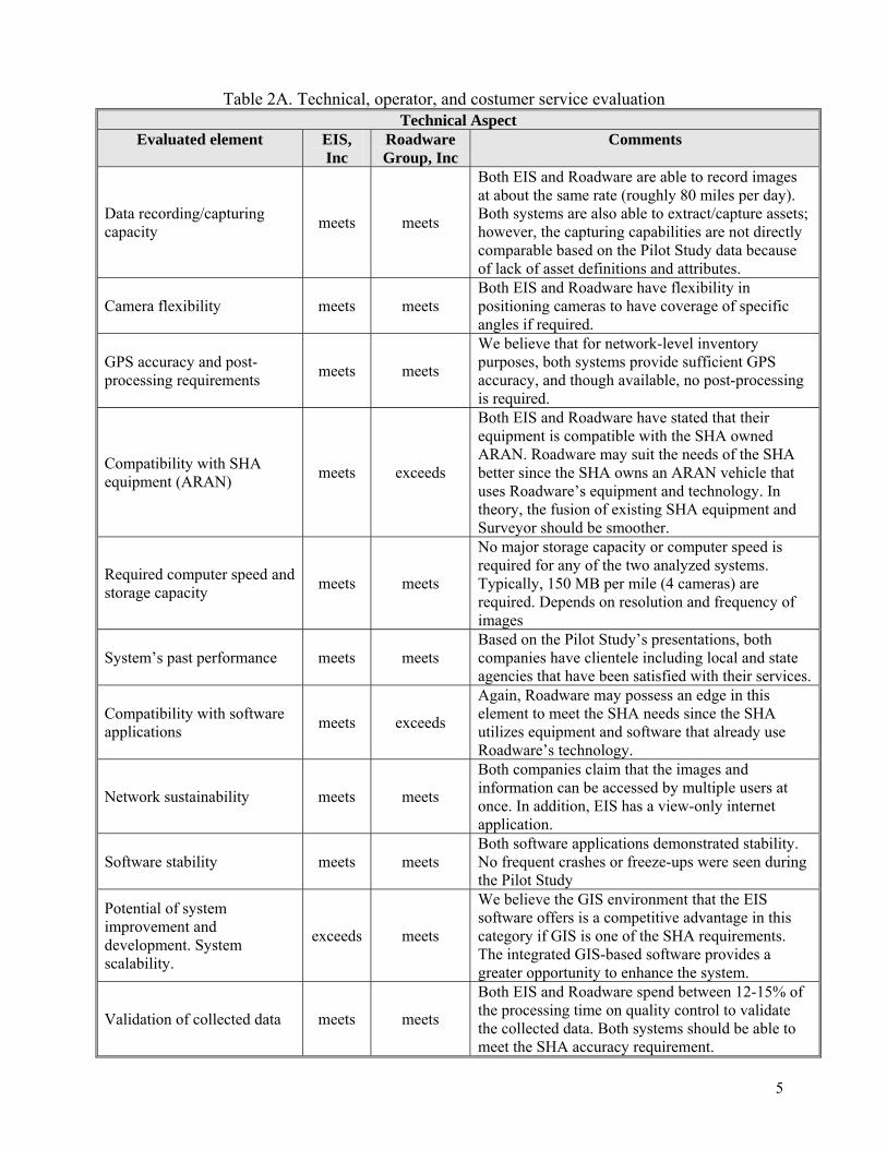
Table 2A. Technical, operator, and costumer service evaluation Technical Aspect

Evaluated element EIS, Inc

Roadware Group, Inc

Comments

Data recording/capturing capacity meets meets

Both EIS and Roadware are able to record images at about the same rate (roughly 80 miles per day). Both systems are also able to extract/capture assets; however, the capturing capabilities are not directly comparable based on the Pilot Study data because of lack of asset definitions and attributes.

Camera flexibility meets meets Both EIS and Roadware have flexibility in positioning cameras to have coverage of specific angles if required.

GPS accuracy and post-processing requirements meets meets

We believe that for network-level inventory purposes, both systems provide sufficient GPS accuracy, and though available, no post-processing is required.

Compatibility with SHA equipment (ARAN) meets exceeds

Both EIS and Roadware have stated that their equipment is compatible with the SHA owned ARAN. Roadware may suit the needs of the SHA better since the SHA owns an ARAN vehicle that uses Roadware’s equipment and technology. In theory, the fusion of existing SHA equipment and Surveyor should be smoother.

Required computer speed and storage capacity meets meets

No major storage capacity or computer speed is required for any of the two analyzed systems. Typically, 150 MB per mile (4 cameras) are required. Depends on resolution and frequency of images

System’s past performance meets meets Based on the Pilot Study’s presentations, both companies have clientele including local and state agencies that have been satisfied with their services.

Compatibility with software applications meets exceeds

Again, Roadware may possess an edge in this element to meet the SHA needs since the SHA utilizes equipment and software that already use Roadware’s technology.

Network sustainability meets meets

Both companies claim that the images and information can be accessed by multiple users at once. In addition, EIS has a view-only internet application.

Software stability meets meets Both software applications demonstrated stability. No frequent crashes or freeze-ups were seen during the Pilot Study

Potential of system improvement and development. System scalability.

exceeds meets

We believe the GIS environment that the EIS software offers is a competitive advantage in this category if GIS is one of the SHA requirements. The integrated GIS-based software provides a greater opportunity to enhance the system.

Validation of collected data meets meets

Both EIS and Roadware spend between 12-15% of the processing time on quality control to validate the collected data. Both systems should be able to meet the SHA accuracy requirement.

5

Table 2A (Continued). Technical, operator, and costumer service evaluation (continued)

Operator Aspect

Evaluated element EIS, Inc

Roadware Group, Inc

Comments

User-friendliness of system exceeds meets

Although Roadware’s software does not present a particular degree of difficulty, in our opinion, the “look and feel” and configuration of Enter-Road-Info seems more straight forward.

Computer skills required meets meets

Basic computer are required for the operation of both software applications in their asset extraction/capturing mode. Further computer skills are needed if the GIS environment is used in Enter-Road-Info (not required for extracting assets).

User customization (assets, attributes, reports) exceeds meets

Both inventory systems are customizable and attributes can be added or changed relatively easy. Enter-Road-Info may possess an edge on meeting the reporting requirements since it has built-in GIS mapping and querying capability

Data processing and capturing exceeds meets

Because it was considered to be more straight forward, we believe that Enter-Road-Info surpasses the data and extraction/capturing process minimum parameter

Additional tools (other than the strictly necessary) exceeds meets

Enter-Road-Info has more readily usable extra features (i.e. measuring tool, grid, best capturing area, etc ) that satisfy the SHA requisites

Capacity of manipulation of data outside of main software meets meets Data from both systems can be exported to most

databases (Microsoft Access generally)

Necessary human resources meets meets Both systems require similar amount of human resources to carry out the recording and extraction/capturing processes

Table 2B. Systems strengths and weaknesses

System Strengths Weaknesses Enter-Road-Info

• Built on ArcView platform. The user has the option of using GIS mapping and querying capabilities • Employs both single image and dual image stereoscopic extraction • Ability to take measurement from one image only • Well organized route sequence storage system

• Extraction procedure leaves no visible reference on captured asset • Interface contains ArcView buttons that may not be used during asset collection

Surveyor • Full administrative structure set up. This provides the ability to login and sign out work to be able to track progress • Easy identification of captured assets on images

• No GIS mapping or querying capability • System is based on multiple windows levels for each task

6

V - Cost Information The cost estimates being presented in this report were provided by EIS, Roadware, and OOM without any standard structure or format; thus, they are not directly comparable. Because of this, ARA took the liberty of performing additional calculations and transformations to be able to compare costs based on comparable units and rates. By way of clarification, it is important to explain how the cost information was developed by the companies and then provided to ARA. EIS provided costs based on the time and resources that were utilized to complete the Pilot Study. EIS then extrapolated these costs to a network level. The information was given to us in a comprehensive report. On the other hand, Roadware gave direct costs based on the size of network and expected number of assets to be collected. This information was provided via e-mail to Mark Chapman (from the SHA Office of Materials Technology) who then forwarded it to ARA. OOM supplied a total figure and a time ratio for the hours spent collecting data out in the field and in the office during this Pilot Study. EIS Cost Information As mentioned before, EIS provided a detailed table with the cost and time utilized to complete the Pilot Study. The costs are summarized in Table 3 (detailed costs can be found in Appendix D):

Table 3. EIS’s provided costs and rates

Phase Pilot Study Cost Network Cost* Image Recording Unavailable $ 600,000 EIS, Inc

Asset Extraction/Capturing $253/ mile $ 2,600,000 Total $ 3,200,000 * Based on 10,266 total miles (5,133 centerline miles). EIS costs include 15% for QC and 5% for project management. Table 4 presents rates that were derived using additional cost and time information provided by EIS.

Table 4. EIS’s derived costs and rates in Pilot Study

Information Provided Derived Rates • Time of image recording = 4 hrs • Length of Pilot Study = 43 miles • Expected time to record images = 6 to 8 months • Time spent on extraction/capturing process = 180.5 hrs • Costs include 15% for QC

• Avg. recording rate ≈ 10 mi/hr (80 mi/day)* • Avg. cost (extraction/capturing only) ≈ $3.22/asset • Estimated miles/week to finish in 7 months assuming 10% downtime (image recording only) ≈ 71 mi/day** • Average capture time ≈ 3.1 min/asset • Estimated image recording cost* ≈ $58.4/ mile

* Rate may be affected by traffic and normal stop and go occurrences ** Based on 10,266 total miles (5,133 centerline miles)

7

Roadware Cost Information As compared with EIS that broke down the cost of the Pilot Study to come up with its network cost estimate, Roadware provided “direct” per-mile cost information on recording and extracting/processing all data, and also for performing the asset extraction/capturing for the entire network. This information is presented in Table 5.

Table 5. Roadware’s provided costs and rates

Phase Provided Cost Total Network Cost* Image Recording and

Asset Extraction/Capturing $105 /mile $ 1,077,720 Roadware Group, Inc

Asset Extraction/Capturing only $70 /mile $ 718,840

* Based on 10,264 total miles (5,132 center miles) and assuming 700,000 assets in the network The following rates were derived using additional cost and time information provided by Roadware. Also, Roadware offered some suggestions should the SHA decide to record the image data. This information is presented in Table 6.

Table 6. Roadware’s derived costs and rates

Information Provided Derived Rates* • Cost of recording and extracting/capturing = $105 /mile • Cost extracting/capturing = $70 /mile • Expected recording rate = 78.8 mi/day • Ratio of 1 QC to 6 to 8 processing staff • Estimate 1.5 minutes to capture asset (40 features/ hr)

• Average cost (recording and extracting/capturing) ≈ $1.54/asset • Average cost (extracting/capturing) ≈ $1.03/asset • Average recording rate ≈ 9.8 mi/hr • Consider 12% to 16% for QC • Estimated image recording ≈ $35/ mile

* Based on 10,264 total miles (5,132 center miles) and assuming 700,000 assets in the network Office of Maintenance Cost Information OOM submitted two lump sums that account for the OOM personnel who worked on the inventory survey for this Pilot Study. Additionally, OOM stated that there was a 1 to 3 hour ratio of time spent in the field to the office. Table 7 shows the cost information provided by OOM.

Table 7. OOM’s derived costs and rates

Information Provided Derived Rates* • First effort = $6,893 • Second effort = $2,965 • Total cost = $9,858

• Field data collection ≈ $2,464 • Office data processing ≈ $7,393 • Field data collection ≈ $57.3 /mile • Office data processing ≈ $171.9 /mile • Total collection and processing ≈ $229.2 /mile

* Based on 43 total miles (Pilot Project)

8

Cost Comparisons As discussed before, different rates were derived from the information provided so costs can be reasonably compared. ARA considered that unit cost per mile was a good estimator to calculate individual task and overall costs. Figure 1 shows a summary of the break down cost per mile based on the derived information. We should caution SHA against using this information as absolute costs to perform the surveys over the entire network. It appears to us that EIS and Roadware used different assumptions in arriving at their projected network level costs. Although these costs provide an order of magnitude level of effort to perform the full network survey, further refinement and analysis would be needed to derive a more pertinent cost to SHA for performance of the surveys.

Figure 1- Summary costs per mile

From the above information, Table 8 presents approximate costs based on an estimated 10,500 SHA network miles.

Table 8. Network cost estimates

Asset Inventory System

Cost per mile (recording and extraction)

Network Cost (approx)

EIS $311.7/ mile $3,272,850 Roadware $105/ mile $1,102,500 OOM $229.2/ mile $2,406,600

Estimated Data Recording Costs

58.4

35

57.3

010203040506070

EIS Roadware OOM

$/m

ile

Estimated Asset Extraction/Capturing Costs

253.5

70

171.9

0

50

100

150

200

250

300

EIS Roadware OOM

$/m

ile

Estimated Total Costs

311.7

105

229.2

050

100150200250300350

EIS Roadware OOM

$/m

ile

9

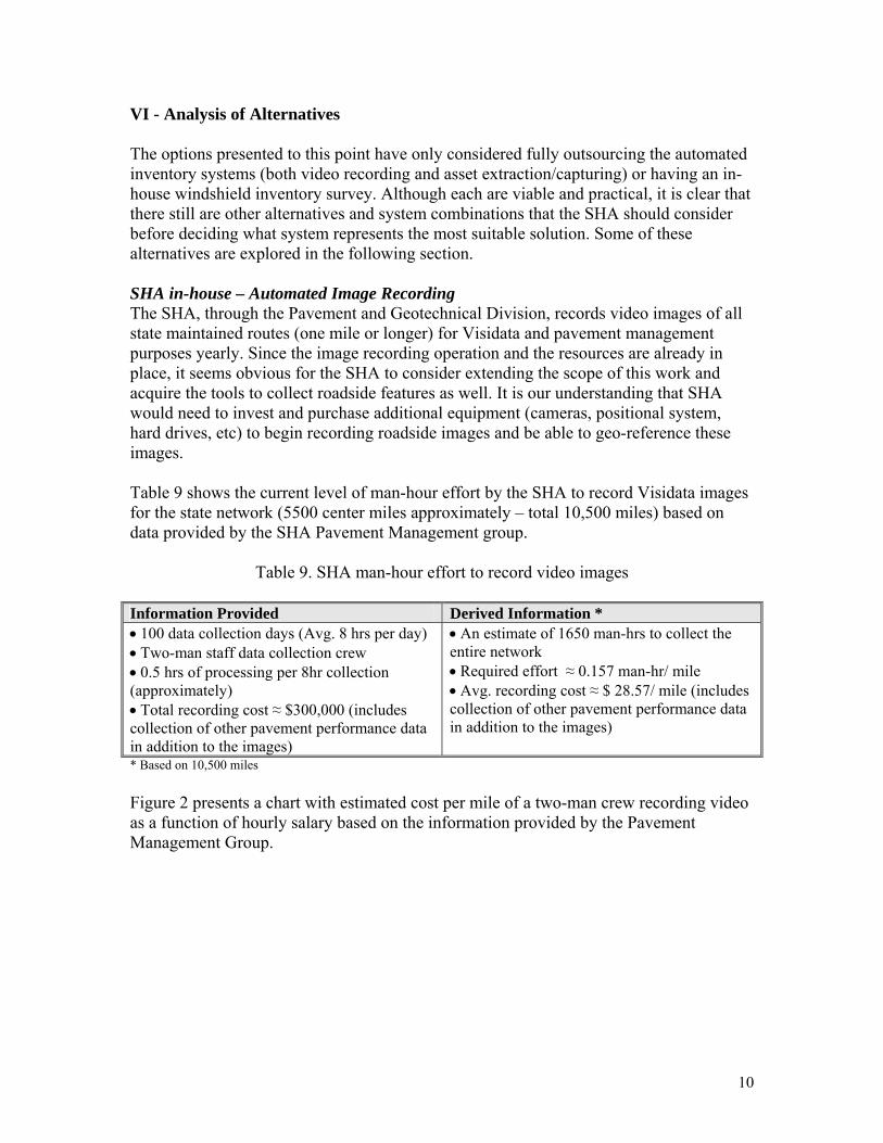
VI - Analysis of Alternatives The options presented to this point have only considered fully outsourcing the automated inventory systems (both video recording and asset extraction/capturing) or having an in-house windshield inventory survey. Although each are viable and practical, it is clear that there still are other alternatives and system combinations that the SHA should consider before deciding what system represents the most suitable solution. Some of these alternatives are explored in the following section. SHA in-house – Automated Image Recording The SHA, through the Pavement and Geotechnical Division, records video images of all state maintained routes (one mile or longer) for Visidata and pavement management purposes yearly. Since the image recording operation and the resources are already in place, it seems obvious for the SHA to consider extending the scope of this work and acquire the tools to collect roadside features as well. It is our understanding that SHA would need to invest and purchase additional equipment (cameras, positional system, hard drives, etc) to begin recording roadside images and be able to geo-reference these images. Table 9 shows the current level of man-hour effort by the SHA to record Visidata images for the state network (5500 center miles approximately – total 10,500 miles) based on data provided by the SHA Pavement Management group.

Table 9. SHA man-hour effort to record video images

Information Provided Derived Information * • 100 data collection days (Avg. 8 hrs per day) • Two-man staff data collection crew • 0.5 hrs of processing per 8hr collection (approximately) • Total recording cost ≈ $300,000 (includes collection of other pavement performance data in addition to the images)

• An estimate of 1650 man-hrs to collect the entire network • Required effort ≈ 0.157 man-hr/ mile • Avg. recording cost ≈ $ 28.57/ mile (includes collection of other pavement performance data in addition to the images)

* Based on 10,500 miles Figure 2 presents a chart with estimated cost per mile of a two-man crew recording video as a function of hourly salary based on the information provided by the Pavement Management Group.

10

Estimate of Cost per Mile of a Two-man Crew

02468

1012141618

0 5 10 15 20 25 30 35 40 45 50 55

Salary ($/hr)

Cos

t ($/

mile

)

Figure 2. Cost per mile of a two-man crew recording video

As mentioned previously, the equipment and operational costs would need to be added to the crew cost in order to have a comprehensive per mile cost. Only then, can the SHA image recording effort be compared to the costs in Table 8. It is important to note that the current image recording cost for Visidata and other pavement performance parameters is $300,000 which translates to $28.57/ mile as shown on Table 9. SHA in-house – Asset Extraction/Capturing For the purpose of evaluating an SHA in-house asset extraction option, ARA reviewed an arbitrarily selected series of roads and assets. ARA staff used both software applications to confirm the validity and accuracy of the inventoried data. In addition we also timed our efforts on the asset extraction/capturing process for the selected roads. The results of this exercise are shown in Appendix E. Should SHA decide to perform the extraction/capturing process in-house, we estimate that its staff should be able to capture assets at an average rate of 6 to 7 minutes/ mile. It is important to note that this rate is based on the individual inventory software applications used and on the number of assets and attributes included in this Pilot Study. Additionally, the rate may vary depending on the abilities of the user and computer capacity or speed. We consider that the 6 to 7 minutes/ mile rate (9 assets) is reasonable for general estimating purposes. Figure 3 provides an estimate of the extraction/capturing process as a function of hourly salary (based on a 6 and 7 min/ mile extraction rate). With this information, the SHA should be able to estimate the raw labor cost of asset extraction/capturing for its network of 10,500 mi. and subsequently add the cost of the software and computer equipment that may be required.

11

Estimate of Cost per Mile of Asset Extraction/Capturing

0123456

0 5 10 15 20 25 30 35 40 45 50 55

Salary ($/hr)

Cos

t ($/

mile

)

6 min/mile7 min/mile

Figure 3. Estimated cost per mile of asset extraction/capturing process For example, using Figure 2 and 3, and assuming an hourly rate of $30/hr, one could estimate the cost of a two-man crew recording images as $10/mile, and $3.5/mile for asset extraction/capturing respectively. The total estimated cost for the SHA would be $141,750 approximately ($13.5/mile, considering a network of 10,500 mi) plus all operational costs (equipment, computer, gas, maintenance, supplies, etc) and additional staff required for QC and support. This is a very simplistic analysis that may not take into account many factors unknown to ARA, however, it should provide a frame of reference for SHA further investigation. VII - SHA Needs Assessment Once the potential costs have been established, it is imperative for the SHA to define and delineate some important aspects regarding its present requirements and needs before taking any further steps. Addressing these aspects would provide helpful insight for the selection of the best inventory system that fulfills the SHA needs, and for the eventual implementation of a complete asset management system. Identification of Required Operational Level To help the SHA identify the kind of system that would best satisfy its requirements, ARA has classified general automated data collection systems for this Pilot Study into three Operational Levels depending on the capacity of the software applications: • Viewer Level – This is the elemental level in which the user is able to play back images. Location reference of the images may be available to the user. No data can be extracted using the recorded images. • Capturing Level – In this level, the user is able to extract linear and point features from the images into a database in addition to the viewing capabilities. Multiple feature attributes and location references such as Global Positioning System (GPS) coordinates

12

can be captured in the database. A comprehensive asset inventory can be put together at this level. Information can be exported to other software applications. • Querying and Mapping Level – In addition to the capabilities in the two previous levels, this level allows the user to have querying and mapping capabilities within the same software application. This intermediate level may integrate GIS or similar technologies. Data from databases can also be exported to other software applications Since the ultimate objective of the SHA is the realization of an inventory system as well as the implementation of a broad asset management system, may want to consider the type of asset management system may best meet its needs and determine what information is needed from its extraction/capturing software. This effort considers the system’s capability of using information obtained from the recorded images and its interaction with models to generate new data; in other words, an actual asset management system. • Interaction and Computation program– has indices to denote current network condition, projections based on performance models, and maintenance and rehabilitation strategies based on budget allocations. Identification of Requirements and Desirable Functions The success of the software application or system chosen will be directly tied to its ability to meet SHA requirements; thus, these requirements and desirable functions need to be defined. If the inventory system’s requirements and the desirable functions are identified, then the more appropriate operational level for the SHA needs will be easier to identify as well. The two types of inventory extraction programs ARA evaluated have numerous similarities; the differences however, may lie in the features that may or may not be considered extra to the SHA’s needs. Table 10 lists examples of features that provide SHA with a choice but may also come at a higher cost. As part of this decision process, it would be important for the SHA to identify the cost implications of the various systems. In theory, the best system for the SHA will be one that meets all of the requirements and also has some desirable functions at an acceptable cost.

Table 10. Requirements or desirable functions

System Difference Requirement or Desirable Function (DF)?

Willing to pay differential cost?

Option for both single or dual stereoscopic image extraction Requirement DF Yes No

Capability single image measurement tools Requirement DF Yes No

Built-in GIS mapping capability and “real time” comparison with aerials

Requirement DF Yes No

Built-in GIS query and reporting capability Requirement DF Yes No

13

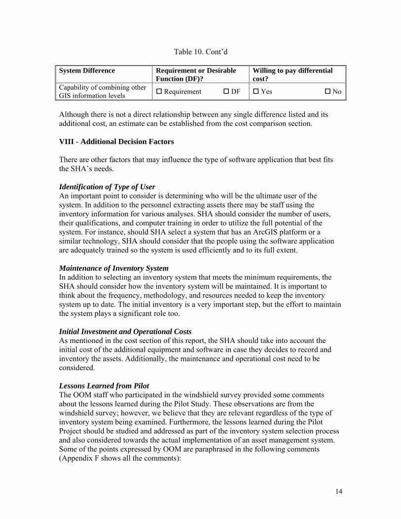
Table 10. Cont’d

System Difference Requirement or Desirable Function (DF)?

Willing to pay differential cost?

Capability of combining other GIS information levels Requirement DF Yes No

Although there is not a direct relationship between any single difference listed and its additional cost, an estimate can be established from the cost comparison section. VIII - Additional Decision Factors There are other factors that may influence the type of software application that best fits the SHA’s needs. Identification of Type of User An important point to consider is determining who will be the ultimate user of the system. In addition to the personnel extracting assets there may be staff using the inventory information for various analyses. SHA should consider the number of users, their qualifications, and computer training in order to utilize the full potential of the system. For instance, should SHA select a system that has an ArcGIS platform or a similar technology, SHA should consider that the people using the software application are adequately trained so the system is used efficiently and to its full extent. Maintenance of Inventory System In addition to selecting an inventory system that meets the minimum requirements, the SHA should consider how the inventory system will be maintained. It is important to think about the frequency, methodology, and resources needed to keep the inventory system up to date. The initial inventory is a very important step, but the effort to maintain the system plays a significant role too. Initial Investment and Operational Costs As mentioned in the cost section of this report, the SHA should take into account the initial cost of the additional equipment and software in case they decides to record and inventory the assets. Additionally, the maintenance and operational cost need to be considered. Lessons Learned from Pilot The OOM staff who participated in the windshield survey provided some comments about the lessons learned during the Pilot Study. These observations are from the windshield survey; however, we believe that they are relevant regardless of the type of inventory system being examined. Furthermore, the lessons learned during the Pilot Project should be studied and addressed as part of the inventory system selection process and also considered towards the actual implementation of an asset management system. Some of the points expressed by OOM are paraphrased in the following comments (Appendix F shows all the comments):

14

Asset definition – there were not clear instructions as to what and how to capture the asset information. The Pilot Study identified some attributes and units but the information was not sufficient. For instance, OOM noticed that the instructions did not provide enough guidelines for signs located at intersections of state and non-state roads. EIS, Roadware, as well as the OOM claimed that line striping was especially hard to account for during their Pilot Study presentations. There was confusion about the brush and tree data collection too. It was not completely clear if it was required to capture only the length that was impeding or obstructing a sign, light, guardrail, etc. at that particular time, or capture any area that could potentially block a roadside feature. Safety – One of the main advantages of using an automated data collection system is safety. Often, field personnel need to step out of the vehicles to collect or verify data, being exposed to other passing vehicles. Many roads in the state network have significant traffic and the risk of having accidents may be reduced by riding the road collecting images. Jurisdiction – It was difficult to determine the right of way and what assets are actually maintained and owned by the SHA. OOM had difficulties identifying features that are the property of the SHA. Utility Companies – Utility companies also maintain their facilities and the SHA does not do any work unless it’s blocking signs or other roadside features. Location accuracy – OOM had some problems trying to provide exact locations for many of the collected assets. Even though the crew was using a DMI, it was difficult to obtain the position of the features. Maintenance Contracts – OOM pointed out that since maintenance contracts are mainly driven by quantities, having a reliable inventory may help to better establish a maintenance plan and a more accurate estimate of the budget needed for the contracts. Reinstallation of Roadside Features – OOM also mentioned how valuable the images and inventory could be if a disaster or accident destroyed a portion of a roadway. Having images and quantities of what was in place would help to establish pre-existing conditions and also with insurance claims. Procedure efficiency – The OOM operation may not be very efficient. The driver is unable to do anything but drive and one person can only do one feature at a time and on one side of the road. As mentioned previously, there also seemed to be a need for a fair amount of stopping along the road to capture all of the information needed in the evaluation. This created a significant inefficiency in the process. Site visits versus image reviewing – The OOM had to revisit some sites to gather additional data or clarify some information. The automated systems are more efficient in this regard since the images are readily available and can be played at any time.

15

IX – Recommendations The Pilot Study provided an excellent forum for SHA to take the fist step towards an asset inventory and ultimately the implementation of an asset management system. Based on our participation in the pilot effort, we offer the following recommendations: SHA should consider developing a plan for an asset inventory that is consistent with the objectives of the asset management system implementation, and that addresses the specific requirements and uses of the data needed. As part of this plan the SHA should… • Identify the required assets and clearly define the specific associated attributes and/or

features for the inventory database • Consider who will be using the data and what type of privileges/rights these users

will have over the data • Create a document that defines the criteria and guidelines for asset characterization

and extraction/capturing. This document should focus on defining and identifying assets and specific rules to extract/capture them, so the information has an acceptable degree of consistency

• Develop a training program for the SHA staff that would be involved in the asset

inventory and asset management system implementation. This training program would explain the general aspects and benefits of implementing an asset inventory and asset management system and the key role that they would play in this implementation

• Select the appropriate asset inventory system based on operational level that would

satisfy SHA’s data requirements ensuring that the application includes the minimum inventory system requirements and desirable functions

• Define the asset inventory system maintenance procedures and policies X – Conclusion In addition to the systems evaluated in this Pilot Study, the SHA has several different alternatives regarding software applications to either inventory assets or implement a full asset management system. Some of these options are listed below: Trident-3D Analyst – asset inventory www.geo-3d.com/products/t3danalyst.html Intergraph – asset inventory www.intergraph.com/road/assetmgt.asp

16

http://www.geo-3d.com/products/t3danalyst.html

http://www.intergraph.com/road/assetmgt.asp

Deighton – asset (infrastructure) management www.deighton.com CarteGraph – asset (infrastructure) management www.cartegrap.com Maximo – general asset management www.mro.com

17

http://www.deighton.com/

http://www.cartegrap.com/

http://www.mro.com/

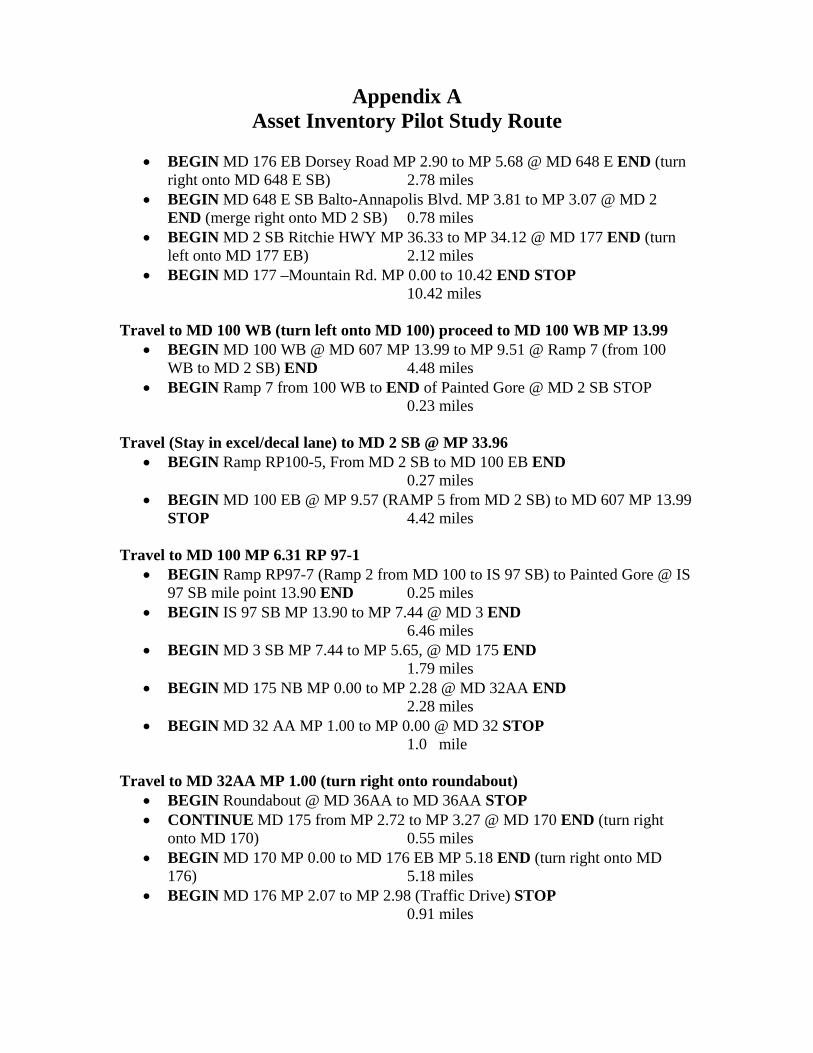
Appendix A Asset Inventory Pilot Study Route

• BEGIN MD 176 EB Dorsey Road MP 2.90 to MP 5.68 @ MD 648 E END (turn

right onto MD 648 E SB) 2.78 miles • BEGIN MD 648 E SB Balto-Annapolis Blvd. MP 3.81 to MP 3.07 @ MD 2

END (merge right onto MD 2 SB) 0.78 miles • BEGIN MD 2 SB Ritchie HWY MP 36.33 to MP 34.12 @ MD 177 END (turn

left onto MD 177 EB) 2.12 miles • BEGIN MD 177 –Mountain Rd. MP 0.00 to 10.42 END STOP

10.42 miles Travel to MD 100 WB (turn left onto MD 100) proceed to MD 100 WB MP 13.99

• BEGIN MD 100 WB @ MD 607 MP 13.99 to MP 9.51 @ Ramp 7 (from 100 WB to MD 2 SB) END 4.48 miles

• BEGIN Ramp 7 from 100 WB to END of Painted Gore @ MD 2 SB STOP 0.23 miles Travel (Stay in excel/decal lane) to MD 2 SB @ MP 33.96

• BEGIN Ramp RP100-5, From MD 2 SB to MD 100 EB END 0.27 miles

• BEGIN MD 100 EB @ MP 9.57 (RAMP 5 from MD 2 SB) to MD 607 MP 13.99 STOP 4.42 miles

Travel to MD 100 MP 6.31 RP 97-1

• BEGIN Ramp RP97-7 (Ramp 2 from MD 100 to IS 97 SB) to Painted Gore @ IS 97 SB mile point 13.90 END 0.25 miles

• BEGIN IS 97 SB MP 13.90 to MP 7.44 @ MD 3 END 6.46 miles

• BEGIN MD 3 SB MP 7.44 to MP 5.65, @ MD 175 END 1.79 miles

• BEGIN MD 175 NB MP 0.00 to MP 2.28 @ MD 32AA END 2.28 miles

• BEGIN MD 32 AA MP 1.00 to MP 0.00 @ MD 32 STOP 1.0 mile

Travel to MD 32AA MP 1.00 (turn right onto roundabout)

• BEGIN Roundabout @ MD 36AA to MD 36AA STOP • CONTINUE MD 175 from MP 2.72 to MP 3.27 @ MD 170 END (turn right

onto MD 170) 0.55 miles • BEGIN MD 170 MP 0.00 to MD 176 EB MP 5.18 END (turn right onto MD

176) 5.18 miles • BEGIN MD 176 MP 2.07 to MP 2.98 (Traffic Drive) STOP

0.91 miles

Appendix B Evaluation Parameters

Technical Aspect

Evaluated Element Evaluation Parameter

Data recording/capturing capacity

System able to record video images of the roadway at the posted speed. System able to extract the selected linear and point roadway assets from the recorded images.

Camera flexibility System able to position more than one camera in the vehicle at different angles to record roadside assets

GPS accuracy and post-processing requirements

System able to locate and establish the position of assets with GPS coordinates at a network level accuracy (less than one meter).

Compatibility with SHA equipment (ARAN)

System able to work and connect efficiently with existing MD SHA equipment, minimizing the acquisition of new hardware and/or software.

Required computer speed and storage capacity

System able to save captured data and process it with traditional computer processors, hardware, and software

System’s past performance System able to demonstrate relevant past performances and that the system has been used successfully implemented in other projects

Compatibility with software applications

System able to demonstrate compatibility with hardware and software applications currently used by MDSHA

Network sustainability System able to accommodate multiple users at the same time. Software stability System able to run without software crashes and freeze-ups. Potential of system improvement and development: System Scalability

Hypothetical in-place system able to add basic and advanced features as well as incorporate new technologies without complete system replacement.

Validation of collected data System includes a quality control process to corroborate captured information.

Operator Aspect Evaluated Element Evaluation Parameter

User-friendliness of system System possesses a simple-to-follow and understandable methodology. System able to work with a straight forward approach.

Computer skills required System able to be used by MD SHA staff possessing basic computer skills (use of mouse and understanding of pull down windows and menus).

User customization (assets, attributes, reports)

System able to be customized by user to meet certain data and information requirements and reporting formats.

Data processing and capturing System able to be direct and straight forward in data and capturing processes.

Additional tools (other than the strictly necessary)

System able to provide not essential tools to aid the user to obtain additional asset information.

Capacity of manipulation of data outside of main software

System able to export data so it can be manipulated and transformed using other software applications.

Necessary human resources System owner able to supply the human resources required to effectively run the complete system process.

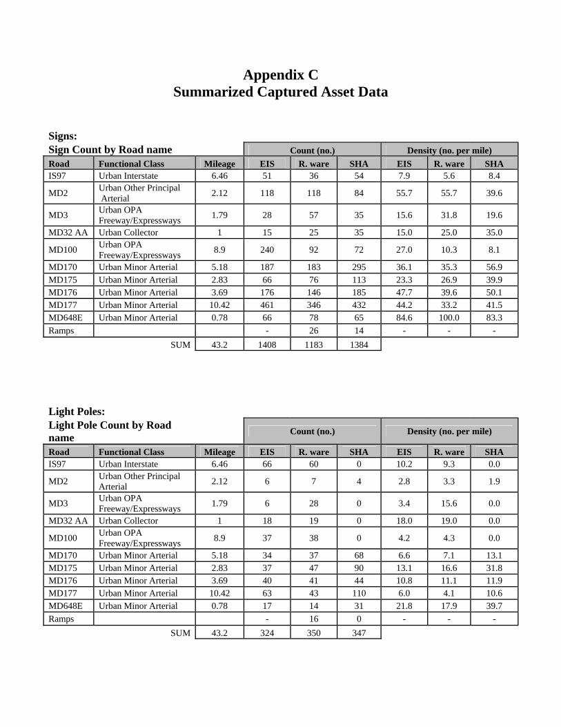
Appendix C Summarized Captured Asset Data

Signs: Sign Count by Road name Count (no.) Density (no. per mile) Road Functional Class Mileage EIS R. ware SHA EIS R. ware SHA IS97 Urban Interstate 6.46 51 36 54 7.9 5.6 8.4

MD2 Urban Other Principal Arterial 2.12 118 118 84 55.7 55.7 39.6

MD3 Urban OPA Freeway/Expressways 1.79 28 57 35 15.6 31.8 19.6

MD32 AA Urban Collector 1 15 25 35 15.0 25.0 35.0


MD170 Urban Minor Arterial 5.18 187 183 295 36.1 35.3 56.9 MD175 Urban Minor Arterial 2.83 66 76 113 23.3 26.9 39.9 MD176 Urban Minor Arterial 3.69 176 146 185 47.7 39.6 50.1 MD177 Urban Minor Arterial 10.42 461 346 432 44.2 33.2 41.5 MD648E Urban Minor Arterial 0.78 66 78 65 84.6 100.0 83.3 Ramps - 26 14 - - - SUM 43.2 1408 1183 1384

Light Poles: Light Pole Count by Road name

Count (no.) Density (no. per mile)

Road Functional Class Mileage EIS R. ware SHA EIS R. ware SHA IS97 Urban Interstate 6.46 66 60 0 10.2 9.3 0.0

MD2 Urban Other Principal Arterial 2.12 6 7 4 2.8 3.3 1.9


MD32 AA Urban Collector 1 18 19 0 18.0 19.0 0.0


MD170 Urban Minor Arterial 5.18 34 37 68 6.6 7.1 13.1 MD175 Urban Minor Arterial 2.83 37 47 90 13.1 16.6 31.8 MD176 Urban Minor Arterial 3.69 40 41 44 10.8 11.1 11.9 MD177 Urban Minor Arterial 10.42 63 43 110 6.0 4.1 10.6 MD648E Urban Minor Arterial 0.78 17 14 31 21.8 17.9 39.7 Ramps - 16 0 - - - SUM 43.2 324 350 347

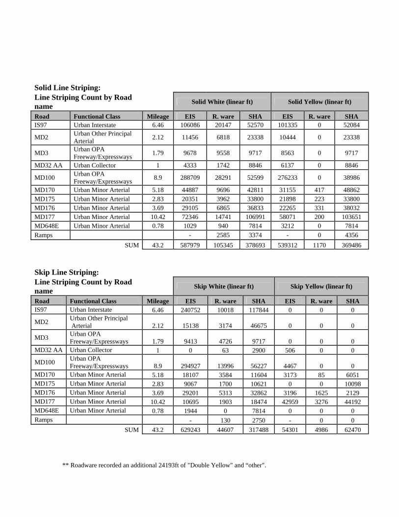
Solid Line Striping: Line Striping Count by Road name

Solid White (linear ft) Solid Yellow (linear ft)

Road Functional Class Mileage EIS R. ware SHA EIS R. ware SHA IS97 Urban Interstate 6.46 106086 20147 52570 101335 0 52084

MD2 Urban Other Principal Arterial 2.12 11456 6818 23338 10444 0 23338

MD3 Urban OPA Freeway/Expressways 1.79 9678 9558 9717 8563 0 9717

MD32 AA Urban Collector 1 4333 1742 8846 6137 0 8846


MD170 Urban Minor Arterial 5.18 44887 9696 42811 31155 417 48862 MD175 Urban Minor Arterial 2.83 20351 3962 33800 21898 223 33800 MD176 Urban Minor Arterial 3.69 29105 6865 36833 22265 331 38032 MD177 Urban Minor Arterial 10.42 72346 14741 106991 58071 200 103651 MD648E Urban Minor Arterial 0.78 1029 940 7814 3212 0 7814 Ramps - 2585 3374 - 0 4356 SUM 43.2 587979 105345 378693 539312 1170 369486

Skip Line Striping: Line Striping Count by Road name

Skip White (linear ft) Skip Yellow (linear ft)

Road Functional Class Mileage EIS R. ware SHA EIS R. ware SHA IS97 Urban Interstate 6.46 240752 10018 117844 0 0 0

MD2 Urban Other Principal Arterial 2.12 15138 3174 46675 0 0 0


MD32 AA Urban Collector 1 0 63 2900 506 0 0


MD170 Urban Minor Arterial 5.18 18107 3584 11604 3173 85 6051 MD175 Urban Minor Arterial 2.83 9067 1700 10621 0 0 10098 MD176 Urban Minor Arterial 3.69 29201 5313 32862 3196 1625 2129 MD177 Urban Minor Arterial 10.42 10695 1903 18474 42959 3276 44192 MD648E Urban Minor Arterial 0.78 1944 0 7814 0 0 0 Ramps - 130 2750 - 0 0 SUM 43.2 629243 44607 317488 54301 4986 62470

** Roadware recorded an additional 24193ft of "Double Yellow" and “other".

Mowable Acres: Mowable Acres Count by Road name Count (no.) Mowable Area (square ft)

Road Functional Class Mileage EIS R. ware SHA EIS R. ware SHA

IS97 Urban Interstate 6.46 21 36 - 1143544 89406 1184324

MD2 Urban Other Principal Arterial 2.12 30 29 - 443635 25278 429235

MD3 Urban OPA Freeway/Expressways 1.79 9 14 - 92132 5668 279300

MD32 AA Urban Collector 1 2 4 - 13144 5171 26525


MD170 Urban Minor Arterial 5.18 57 29 - 273438 15702 167942 MD175 Urban Minor Arterial 2.83 17 4 - 42595 1196 88147 MD176 Urban Minor Arterial 3.69 30 22 - 155278 10008 746909 MD177 Urban Minor Arterial 10.42 120 121 - 232605 21381 437760 MD648E Urban Minor Arterial 0.78 4 4 - 6175 238 0 Ramps 2 - - 3169 5383

SUM 43.2 354 310 - 12044041 305269 6460027

Brush and Tree: Brush and Tree Count by Road name

Count (no.) Brush (linear ft)

Road Functional Class Mileage EIS R. ware SHA EIS R. ware SHA IS97 Urban Interstate 6.46 0 0 - 0 0 37646





MD170 Urban Minor Arterial 5.18 0 2 - 0 7578 12204 MD175 Urban Minor Arterial 2.83 0 1 - 0 1459 13179 MD176 Urban Minor Arterial 3.69 0 0 - 0 0 2200 MD177 Urban Minor Arterial 10.42 12 4 - 1378 25923 31912 MD648E Urban Minor Arterial 0.78 0 1 - 0 678 0 Ramps - 0 - 0 528 SUM 43.2 14 8 - 1603 35637 588457

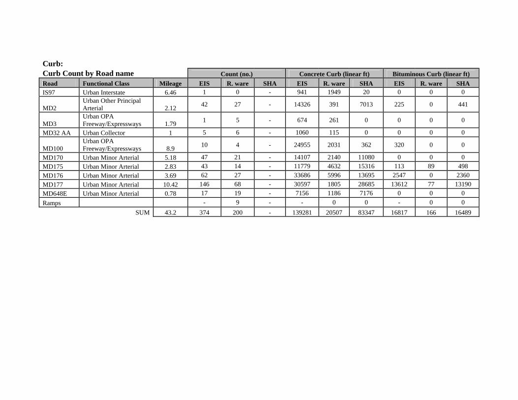
Curb: Curb Count by Road name Count (no.) Concrete Curb (linear ft) Bituminous Curb (linear ft) Road Functional Class Mileage EIS R. ware SHA EIS R. ware SHA EIS R. ware SHA IS97 Urban Interstate 6.46 1 0 - 941 1949 20 0 0 0

MD2 Urban Other Principal Arterial 2.12 42 27 - 14326 391 7013 225 0 441

MD3 Urban OPA Freeway/Expressways 1.79 1 5 - 674 261 0 0 0 0

MD32 AA Urban Collector 1 5 6 - 1060 115 0 0 0 0

MD100 Urban OPA Freeway/Expressways 8.9 10 4 - 24955 2031 362 320 0 0

MD170 Urban Minor Arterial 5.18 47 21 - 14107 2140 11080 0 0 0 MD175 Urban Minor Arterial 2.83 43 14 - 11779 4632 15316 113 89 498 MD176 Urban Minor Arterial 3.69 62 27 - 33686 5996 13695 2547 0 2360 MD177 Urban Minor Arterial 10.42 146 68 - 30597 1805 28685 13612 77 13190 MD648E Urban Minor Arterial 0.78 17 19 - 7156 1186 7176 0 0 0 Ramps - 9 - - 0 0 - 0 0 SUM 43.2 374 200 - 139281 20507 83347 16817 166 16489

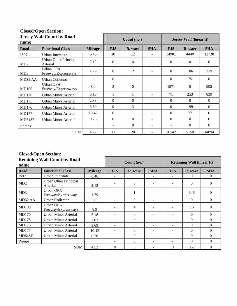
Closed/Open Section: Jersey Wall Count by Road name

Count (no.) Jersey Wall (linear ft)

Road Functional Class Mileage EIS R. ware SHA EIS R. ware SHA IS97 Urban Interstate 6.46 10 12 - 24901 4440 12738





MD170 Urban Minor Arterial 5.18 1 1 - 71 253 839




MD648E Urban Minor Arterial 0.78 0 0 - 0 0 0

Ramps - 0 - - 0 0

SUM 43.2 13 20 - 26542 5150 14894

Closed/Open Section: Retaining Wall Count by Road name

Count (no.) Retaining Wall (linear ft)

Road Functional Class Mileage EIS R. ware SHA EIS R. ware SHA IS97 Urban Interstate 6.46 - 0 - - 0 0

MD2 Urban Other Principal Arterial 2.12 - 0 - - 0 0

MD3 Urban OPA Freeway/Expressways 1.79 - 1 - - 346 0

MD32 AA Urban Collector 1 - 0 - - 0 0

MD100 Urban OPA Freeway/Expressways 8.9 - 4 - - 16 0

MD170 Urban Minor Arterial 5.18 - 0 - - 0 0 MD175 Urban Minor Arterial 2.83 - 0 - - 0 0 MD176 Urban Minor Arterial 3.69 - 0 - - 0 0 MD177 Urban Minor Arterial 10.42 - 0 - - 0 0 MD648E Urban Minor Arterial 0.78 - 0 - - 0 0 Ramps - 0 - - 0 0 SUM 43.2 0 5 - 0 362 0

Closed/Open Section: Bridge Count by Road name Count (no.) Bridge (linear ft) Road Functional Class Mileage EIS R. ware SHA EIS R. ware SHA IS97 Urban Interstate 6.46 3 4 - 758 271 1131





MD170 Urban Minor Arterial 5.18 1 1 - 38 11 0 MD175 Urban Minor Arterial 2.83 0 0 - 0 0 0 MD176 Urban Minor Arterial 3.69 0 0 - 0 0 0 MD177 Urban Minor Arterial 10.42 0 0 - 0 0 0 MD648E Urban Minor Arterial 0.78 0 0 - 0 0 0 Ramps - 0 - - 0 0 SUM 43.2 9 10 - 1631 528 3130

Rout Length (mi) Asset Inventory System

No. of assets identified by

ARA Surveyor 11

MD 32 AA 1 Roadside Signs E-R-I 11 Surveyor 63

IS 97 6.46 Light Poles E-I-S 57 Surveyor 4

MD 175 2.28 Mowable acres E-I-S 6 Surveyor 4

MD 177 10.42 Brush and Tree Encroachment E-R-I 19 Surveyor 4

MD 3 1.79 Curb and Barriers E-R-I 4 Surveyor 51

MD 2 2.12 Pavement Marking E-R-I * distance

Appendix D EIS Cost Table

Feature Type Feature Count

Hours Spent

Feature collected per hour

Hours per mile

Cost per feature

($)

Cost per mile ($) +

15%

Cost per mile ($) +

20%

State-wide Cost

Estimate Signs 1408 60 23.5 1.5 2.30 77.6 84.4 866194

Striping 579 46 12.6 1.15 4.29 59.5 64.7 664082 Curb 498 30 16.6 0.75 3.25 38.8 42.2 433097

Mowing Area 414 23 18.0 0.575 3.00 29.8 32.3 332041 Light Pole 324 9 36.0 0.225 1.50 11.6 12.7 129929 Guardrail 150 10 15.0 0.25 3.60 12.9 14.1 144366

Brush 14 1 14.0 0.025 3.86 1.3 1.4 14437 Jersey Wall 13 1 13.0 0.025 4.15 1.3 1.4 14437

Bridge 9 0.5 18.0 0.0125 3.00 0.6 0.7 7218

Average Cost $ 3.22 $ 233.52 $ 253.83 $2,605,800

Appendix E

Asset Capturing Timing Results

EIS

(time) Roadware

(time) Signs 14' 27" 11' 0" Poles 6' 00" 3' 51" Pavement Markings 6' 52" 13' 12" Curb/Barrier 3' 42" 3' 54" Mowable Area 5' 18" 6' 34" Brush and Tree 4' 20" 4' 07"

Average Rate 6' 47" 7' 06"

Appendix F OOM - Lessons Learned and unanswered questions

Sign Installation • What do we do with the signs that are apparently not ours, but impact our operations? • How do we identify which signs are ours? (Non SHA person) • The inventory does not need to know the number and type of poles, and sign type.

But the data base needs to have the ability to capture that information over time from routine maintenance activities.

• Need rules to count signs. Like....

State road intersecting with a State Road State road intersecting with non-State Road How do we capture signs that are not mounted on a post(s?) Signs that are not ours but we installed and maintain

Light Installations • Need a way to figure out which lights are ours. The assumption on the pilot was if

they were mounted on a wooden pole they were not ours. • Except.... round-a-bouts and streetscapes • Need rules to count lights. Like....

State road intersecting with a State Road State road intersecting with non-State Road

• When the project goes into full swing will need to further define lights.

Can the light head be lowered? Is the light mounted on a common pole used for other things?

Line Striping • Need to determine what we are measuring. Is it Amount of paint on the road?

Amount of work performed? Linear distance (recommended)?

• What about thermal markings? • Ramps need to be measured as a road Oust (just shorter) • For the pilot we began and ended the ramps at the apex of the painted gore. By doing

it that way we had a start and stop point. But missed the puppy tracks because they did not belong to the road or the ramp.

• What about pavement markings? Mowing • What are we measuring? Currently we measure acres mowed. Shouldn't we be

measuring linear feet and calculating the acres? (recommended) • Do we measure what is mowed, what should be mowed, what can be mowed, or

apply the standard and not worry about the actual conditions? • If linear measurements are used we do not have to discriminate on the type of

mowing. The data base will give information about obstructions to mowing (signs, guard rail, etc.). That will dictate the type of activity that needs to be performed.

• Need to define what is mowing. If it can be mowed (wild flower beds) is it mowing?

This goes back to the "what are we measuring" point. • Do we measure mowing that is not on our property? Example:

Areas around utility poles. Assuming the poles delineates the property line; we should only mow to the left of the pole. In reality we mow behind it also.

Brush and Tree • What is brush and tree? • Is it everything that we do not mow? • Does it have to be on our property for it to be counted? • Ways to measure brush and tree

Linear distance times some number. That number would be the amount that we actually have to maintain. Recommend 5 feet. We have brush and tree everywhere we have a road Except where something else is there, like curb, retaining wall, SBW

Open/Closed Roadway delimitation • Need to define what we are measuring. For the pilot we were measuring to determine

maintenance operations, blading vs. sweeping. Is curb

Traffic control Drainage Landscaping (to include side walks and plantings)

By defining why it is there we can later determine if it performing to the designed function. Retaining wall vs. Jersey barrier • Need to inventory based on function not what it looks like

During the pilot we noticed that most retaining wall had a Jersey barrier profile. We counted it a jersey barrier based on the rules of the pilot.

There is Jersey barrier that is actually a retaining wall. Weep holes

• Bridge deck is part of the bridge, so is the retaining wall. This is Bridges inventory. General • Need to define the segments based on roadway type. The features remain fairly

consistent based on the type of road. Then we can populate the data base, and only add or subtract the differences.

• Need clearly defined and mark mile points for start and stop of measurements.

Suggest using landmarks that do not move or change frequently. Example center of mass of a bridge or overpass, center of intersection.

• One person can only do one feature at a time, on one side of the road. • The exception is lights and signs, but still only on one side. • DMI operator is needed • Driver must do nothing but drive • Need to predefine what we are measuring for, and ensure the data is not so specific it

can not be used for other purposes. Example. Line striping. Do we measure the work to apply it, the amount of paint on the road, or the linear distance of the painted lines?

• Need to define assumptions prior to measurement • Need some solid baseline assumptions, based on some facts or standards. Example:

We can assume that there is brush and tree everywhere, except where we mow. We can assume there is ROW fence, except where there is not. Based on road type, we can assume certain painting rules exist.

• There is drainage everywhere; base on road type defines what kind. Then we only

have to measure the exception to the assumptions

• Need to establish solid baseline rules. Like the asset association. What gets counted

with what? Example. A bridge retaining wall next to the interstate. The retaining wall gets associated with the bridge because if it was not there the bridge would be impacted, not the interstate.

• Need a minimum quantity for all assets before they are measured.

Example: If the area between a jersey barrier and a sound barrier wall is 2 feet and there are some plants in there, is it landscaping?

VisiData.

Negative side

Has a 480 foot interval between frames. This interjects a minimum of 240 foot measurement error. Does not measure ramps, service roads. Treats round-a-bouts as a linear road. Mile points do not match Highway reference manual. Difficult if not impossible to differentiate between concrete and bituminous curb based on profile of curb. Difficult if not impossible to see weep holes in the Jersey barrier. This is a key feature to tell us it is actually retaining wall.

Positive side

(Assuming the negative sides can be overcome)

Is not weather dependent for inventory. Is an efficient use of time. Does not require a team effort. Can easily "Back up" and start over. Can possibly do more than one feature at a time. Safer than being on the road.

asset inventory system: pilot · pdf fileasset inventory system: pilot study 6. ... inventory...

Documents