Asset-Liability Management Modelling with Risk Control by

Stochastic Dominance

Xi Yang ∗ Jacek Gondzio † Andreas Grothey ‡

School of Mathematics and Maxwell Institute for Mathematical Sciences

University of Edinburgh

James Clerk Maxwell Building

King’s Buildings

Mayfield Road

Edinburgh EH9 3JZ

U.K.

Technical Report ERGO-09-002, January 15th, 2009

Revised August 2009, December 2009

∗University of Edinburgh, UK, X.Yang@ed.ac.uk, corresponding author†University of Edinburgh, UK‡University of Edinburgh, UK

1

Abstract

An Asset-Liability Management model with a novel strategy for controlling the risk of

underfunding is presented in this paper. The basic model involves multiperiod decisions

(portfolio rebalancing) and deals with the usual uncertainty of investment returns and fu-

ture liabilities. Therefore it is well-suited to a stochastic programming approach. A stochastic

dominance concept is applied to control risk of underfunding through modelling a chance

constraint. A small numerical example and an out-of-sample backtest are provided to demon-

strate the advantages of this new model, which includes stochastic dominance constraints,

over the basic model and a passive investment strategy.

Adding stochastic dominance constraints comes with a price. This complicates the struc-

ture of the underlying stochastic program. Indeed, the new constraints create a link between

variables associated with different scenarios of the same time stage. This destroys the usual

tree-structure of the constraint matrix in the stochastic program and prevents the application

of standard stochastic programming approaches such as (nested) Benders decomposition and

progressive hedging. Instead we apply a structure-exploiting interior point method to this

problem. The specialized interior point solver OOPS can deal efficiently with such problems

and outperforms the industrial strength commercial solver CPLEX on our test problem set.

Computational results on medium scale problems with sizes reaching about one million vari-

ables demonstrate the efficiency of the specialized solution technique. The solution time for

these nontrivial asset liability models appears to grow sublinearly with the key parameters

of the model, such as the number of assets and the number of realizations of the benchmark

portfolio, which makes the method applicable to truly large scale problems.

1 Introduction

The Asset-Liability Management (ALM) problem has crucial importance for pension funds,

insurance companies, and banks whose business involves a large amount of liquidity. Indeed,

these financial institutions apply ALM to guarantee meeting their liabilities while pursuing

profit. The liabilities may take different forms: pensions paid to the members of the scheme

in a pension fund, savers’ deposits paid back in a bank, or benefits paid to insurees in an

insurance company. A common feature of these problems is the uncertainty of liabilities and

asset returns and the resulting risk of underfunding. This constitutes a nontrivial difficulty

in managing risk in any model applied by the financial institution. The need for multi-period

2

planning additionally complicates the problem.

The paradigm of stochastic programming [1, 24] is well-suited to tackle these problems

and has already been applied in this context as shown in [36] and in the many references

therein. One of the first industrially applied models of this type was the stochastic linear

program with simple recourse developed by Kusy and Ziemba in [26]. This model captured

certain characteristics of ALM problems: it maximized revenues for the bank in the objective

under legal, policy, liquidity, cash flow and budget constraints to make sure that deposit

liabilities were met as closely as possible. Under the computational limits at the time when

it was developed, this model took advantage of stochastic linear programming so as to be

practical even for the large problems faced in banks. It was shown to be superior to a

sequential decision theoretical model in terms of maximizing both the initial profit and the

mean profit. However, risk management was not considered in this work: only expected

penalties of constraint violation were taken into account.

A major difficulty in ALM models consists in risk management. One may follow the

Markowitz risk-averse paradigm [28] and trade off multiple contradictory objectives: maxi-

mize the return and minimize the associated risk, e.g. [31]. A successful example of optimization-

based ALM modelling which took risk management issues into account was the Russell-

Yasuda Kasai model for a Japanese insurance company by the Frank Russell consulting

company, which used multi-stage stochastic programming [4, 5]. This dynamic stochastic

model took into account multiple accounts, regulatory rules and liabilities to enable the

managing of complex issues arising in the Yasuda Fire and Marine Insurance company. Ex-

pected shortfall, i.e. the expected amount by which the goals were not achieved, was applied

to measure risk more accurately than the calculation of expected penalties and it was easy

to handle in the solution process. Moreover, the model proved to be easy to understand by

decision-makers. The implementation results showed the advantages of the Russell-Yasuda

model over the mean-variance model in multi-period and multi-account problems.

There are various ways to control risk in addition to the above mentioned such as variance

and value at risk. Stochastic dominance leads to an alternative tool and it has recently gained

substantial interest from the research community. It has several attractive features but two

of them are particularly important: stochastic dominance is consistent with utility functions

and it considers the whole probability distribution. We will discuss these issues in detail

in Section 3. The stochastic dominance concept dates from the work of Karamata in 1932

(see [27] for a survey). Subsequently, stochastic dominance has been applied in statistics [2],

economics [21, 22] and finance. However, stochastic dominance involves the comparison of

3

(nonlinear) probability distribution functions and this makes its straightforward application

difficult.

The inclusion of first-order stochastic dominance within the stochastic programming

framework leads to a non-convex mixed integer programming formulation. By contrast,

second-order stochastic dominance can be incorporated in the form of linearized constraints

[9] which makes it a more attractive option. In a series of papers, Dentcheva and Ruszczynski

analyzed several aspects of the use of stochastic dominance, such as its optimality and du-

ality [9], applications to nonlinear dominance constraints [10] and an application to static

portfolio selection [11]. The introduction of non-convex constraints by the use of first-order

stochastic dominance introduces serious complications into optimization models and makes

their solution difficult. Relaxations of these problems were analyzed in [29]; stability and

sensitivity of first-order stochastic dominance with respect to general perturbation of the

underlying probability measures were studied in [8]. Noyan, et al. in [29] also introduced

interval second-order stochastic dominance which is equivalent to first-order stochastic dom-

inance and generated a mixed integer problem based on this dominance relation. Roman, et

al. proposed a multi-objective portfolio selection model with second-order stochastic dom-

inance constraints [33] and Fabian, et al. [13] developed an efficient method to solve this

model based on a cutting-plane scheme. The application of stochastic dominance in dis-

persed energy planning and decision problems has been illustrated in [15, 16, 17], including

both first-order and second-order stochastic dominance. The use of multivariate stochastic

dominance to measure multiple random varables jointly was discussed in [12].

To the best of our knowledge, stochastic dominance has not yet been applied in the ALM

context and in this paper we demonstrate how this can be done. Further, we introduce relaxed

interval second-order stochastic dominance, which is a dominance constraint intermediate

between first-order and second-order, in a problem with discrete probability distributions,

and demonstrate how it can be used to model chance constraints. By combining second-order

stochastic dominance and relaxed interval second-order stochastic dominance, the model

can help generate portfolio strategies with better management of risk and better control of

underfunding. We illustrate this issue with a small example and an out-of-sample backtest

analysed in Sections 5.1 and 5.2, respectively.

Due to the uncertainties of asset returns and liabilities, the resulting stochastic program-

ming formulation involves many scenarios corresponding to the Monte Carlo simulation of

realisations of the random factors. As a result, the problem grows to a large size, especially

when the problem has multiple stages, and this leads to difficulties in the solution pro-

4

cess. Consigli and Dempster [6] proposed the Computer-aided Asset/Liability Management

(CALM) model as a multi-stage model and solution. Of the simplex method, the interior

point method and nested Benders decomposition, the last one is shown to be the most

efficient in the sense of both solution time and memory requirements.

Stochastic dominance constraints link variables which are associated with different nodes

at the same stage in the event tree. Adding such constraints to the linear stochastic pro-

gramming problem destroys the usual tree-structure of the problem and prevents effective

use of direct Benders decomposition or the progressive hedging algorithm [32]. See [14] for

a solution based on dual decomposition. We discuss this issue further in Section 5.3. In-

stead we apply the specialized structure-exploiting parallel interior point solver OOPS to

the structure of our ALM model with stochastic dominance constraints, to take advantage

of such information in the solution process. OOPS is an interior point solver which uses

object-oriented programming techniques and treats each sub-structure of the problem as

an object carrying its own dedicated linear algebra routines [20]. This design allows OOPS

to deal with complicated ALM problems which contain stochastic dominance constraints.

The computational results confirm that, by exploiting the structure, OOPS outperforms the

commercial optimization solver CPLEX 10.0 on these problems.

The basic multi-stage stochastic programming model used for Asset-Liability Manage-

ment is discussed in Section 2. The theoretical issues of stochastic dominance are discussed in

Section 3 with emphasis on second-order stochastic dominance and relaxed interval second-

order stochastic dominance. The practical aspects of the application of different stochastic

dominance constraints in the ALM model (second-order and relaxed interval second-order

stochastic dominance) are covered in Section 4. These are followed in Section 5 by an analysis

of a small example of the model proposed and a backtest and discussion of computational

results for a selection of realistic medium scale problems. Section 6 concludes the paper.

2 Asset-Liability Management

ALM models assist financial institutions in decision making on asset allocations considering

full use of the fund and resources available. The model aims to maximize the overall revenue,

sometimes as well as revenue at intermediate stages, while controlling risk. Risk in ALM

problems is present in two aspects: a possible loss of investment value and the inability to

meet liabilities. The returns of assets and the liabilities are both uncertain. It is essential

in ALM modelling to deal with these uncertainties as well as with the resulting risks. The

5

stochastic programming approach is naturally applicable to problems which involve basic

uncertainties; an approach to deal with risk management is discussed in the next section.

2.1 Multi-Stage ALM Modelling

Suppose a financial institution plans to invest in assets from a set I = {1, . . . ,m}, with xi

denoting the investment in asset i. The return r of assets is uncertain, but we assume that

it has a known probability distribution, which can be deduced from historical data, and the

total return of the portfolio is R = rTx. Then we can calculate the expected return of the

portfolio:

E[R] =∑

i

E[xi ∗ ri] =∑

i

xiE[ri]. (1)

Considering a risk function φ(x) measuring the risk incurred by decision x ∈ Rm, a general

portfolio selection problem, without taking the liabilities into account, can be formulated in

one of the following three ways:

minx −E[rTx] + φ(x), x ∈ X, (2)

minx φ(x), E[rTx] ≥ α, x ∈ X, (3)

minx −E[rTx], φ(x) ≤ β, x ∈ X. (4)

Suppose that constraints E[rTx] ≥ α, φ(x) ≤ β have strictly feasible points. It can be

proven (see [25]) that these three problems are equivalent in the sense that they can generate

the same efficient frontier, given a convex set X and a convex risk measure function φ(x).

The best-known example of formulation (2) is the Markowitz mean-variance multi-objective

model [28], which considers both return and risk in the objective. In formulation (3) risk is

minimized with acceptable returns, while in formulation (4), the return is maximized subject

to risk being kept at an acceptable level. The constraint in (4) defines the feasible set with

feasible risk so that in the objective the decision-maker can focus on maximizing the return.

In this paper we will use formulation (4).

Besides return and risk control, the ALM model considered has also the following features:

1. Transaction costs; each transaction will be charged a certain percentage of total trans-

action value, and different transaction costs may apply to purchases and sales;

2. Cash balance; liabilities should be paid to clients, meanwhile there is an inflow in terms

of deposits or premiums; the model should make sure the outflow and inflow match;

6

3. Inventories of assets and cash, which are essential in a dynamical system of 2- or even

a multiple - stage problem;

4. Legal and policy constraints aligned with the financial sector’s requirements.

This work considers the first three points.

It is important for the decision makers to rebalance the portfolio during the investment

period as they may wish to adjust the asset allocations according to updated information

on the market. The strategy which is currently optimal may not be optimal any more as the

situation changes. Taking this into account, the problem is a multi-period problem and at

the beginning of each period in the model, new decisions are made.

We denote the time horizon by T , and denote decision stages by t = 0, . . . , T . At each

time stage t a decision is made on the units of each asset to be invested in and amount of

cash held, based on the state of the total wealth and the forecast of prospective performance

of the assets at that particular time. When the random factors follow discrete distributions,

the resulting decision process can be captured by an event tree, as shown in Figure 1. Each

node is labelled with (i, j) denoting node j at stage i. Each node represents a possible future

event. Asset returns, liabilities and cash deposits are subject to uncertain future evolution.

Meanwhile, the asset rebalancing is done after knowing the values which the asset returns

and liabilities take at each node.

(1,2)

(2,1)

(1,1)

(2,5)

(2,4)

(2,3)

(2,2)

(0,1)

t=3t=2t=1

Figure 1: An example of event tree describing different return states of nature.

The notation of the model is given first:

Parameters:

Wi: price of asset i;

G: total initial wealth;

7

λ: the penalty coefficient of underfunding;

γ: the transaction fee, which is proportional to trading volume (assumed to be equal for

purchases and sales);

β: upper bound on acceptable risk;

ψ: funding ratio, showing the percentage of liabilities to be satisfied;

Random data:

Rti,j : the return of asset i in node j at stage t;

Rtc,j : the interest rate in node j at stage t;

Atj : the outflow of resources, e.g. liabilities;

Dtj : the inflow of resources, e.g. contributions;

π: the joint probability distribution of above uncertain factors;

Decision variables:

xhti,j : units of asset i held in node j at stage t;

xsti,j : units of asset i sold in node j at stage t;

xbti,j : units of asset i bought in node j at stage t;

ctj : units of cash held in node j at stage t;

bTj : the amount of underfunding in node j at the terminal stage that cannot be satisfied;

Indexes and sets:

t: the stage index, with t = 1, . . . , T ;

i: the asset index, with i ∈ I = {1, . . . ,m};

nt: the number of nodes at stage t;

j: the node index, with j ∈ Nt = {1, . . . , nt}, t = 1, . . . , T ;

a(j): the ancestor of node j;

Then the multi-stage ALM problem concerning the investment strategy can be represented

as:

max∑

j∈NT

πTj (

∑i∈I

(1− γ)WixhTi,j) + cTj − λbTj (5a)

s.t. (1 + γ)∑i∈I

Wixh0i,0 + c0 = G−A0 +D0 (5b)

(1 + γ)∑i∈I

Wixbti,j + ctj = (1− γ)

∑i∈I

Wixsti,j + (1 +Rt

c,j)ct−1a(j) −At

j +Dtj , (5c)

(1 +Rti,j)xh

t−1i,a(j) + xbti,j − xst

i,j = xhti,j , (5d)

∑i∈I

(1− γ)WixhTi,j + cTj + bTj ≥ ψAT

j , (5e)

8

φ(xhtj , c

tj) ≤ β, (5f)

xhti,j ≥ 0, xst

i,j ≥ 0, xbtj ≥ 0, bTj ≥ 0

xhtj , xst

j , xbtj ∈ Rm

i ∈ I = {1, . . . ,m}, j ∈ Nt = {1, . . . , nt}, t = 1, . . . , T,

where φ(·) gives the risk associated with position (xh, c).

The decision maker does not seek a strategy to strictly satisfy the liability at the horizon

of the problem, but penalises the underfunding. The objective (5a) aims to maximize the final

wealth of the fund taking into account the penalties of underfunding. Equation (5b) balances

the initial wealth at the first stage while (5c) are cash balances for the following stages, both

taking into account transaction costs, proportional to the total trade volume. The inventories

of each asset at each stage are captured in (5d). (5e) defines the underfunding level bj at the

terminal stage. Risk control is expressed in (5f) with the risk measure function φ(·) and the

maximum acceptable level of risk β. This constraint will be discussed in more detail in the

following section. If the risk constraint is linear, the model (5) is a linear program.

Risk control in an ALM problem involves many aspects. Two of the most important are

overall performance and underfunding. The overall performance is analyzed considering all

possible outcomes of the portfolio, e.g. variance. We will use stochastic dominance to control

the risk of overall performance and discuss the modelling issues involved in Section 3.2.

Underfunding concerns the possibility of unsatisfied liabilities only. To avoid underfunding

completely is expensive to implement and in many situations impossible. We will control

underfunding through the stochastic dominance constraints discussed in Section 3.3.

3 Stochastic Dominance

Stochastic dominance, as a risk control tool, has been considered in reference to certain

risk measures by Ogryczak and Ruszczynski in [30, 34]. Below we demonstrate how it can

be incorporated into our ALM model. First we briefly recall the definitions of stochastic

dominance following closely the exposition in [30]. The reader familiar with these definitions

may skip Section 3.1.

9

3.1 Definition and Properties of Stochastic Dominance

Given a random variable ω, we consider the first performance function, which is actually the

probability distribution function, as:

F 1ω(η) = P (ω ≤ η). (6)

Then we say that random variable Y dominates L by first-order stochastic dominance (FSD)

if:

F 1Y (η) ≤ F 1

L(η), ∀η ∈ R, (7)

denoted as

Y �1 L. (8)

Next, we define the second performance function as:

F 2ω(η) =

∫ η

−∞F 1

ω(ζ)dζ, ∀η ∈ R. (9)

Then we say that random variable Y dominates L by second-order stochastic dominance

(SSD) if:

F 2Y (η) ≤ F 2

L(η), ∀η ∈ R, (10)

denoted as

Y �2 L. (11)

Hence, if Y and L are returns of two portfolio strategies satisfying (7) (or (10)), then Y

dominates L and Y is preferable. Iteratively, we can define higher order stochastic dominance.

And it has also been proven that the lower order dominance relations imply the dominance

of higher orders [30, 35].

Stochastic dominance has been used up to the present in decision theory and economics.

The most important reason for this is its consistency with utility theory. Utility measures a

degree of satisfaction. The value of a portfolio depends only on itself and is equal for every

investor; the utility, however, is dependent on the particular circumstances of the person

making the estimate. Investors seek to maximize their utilities. In general, utility functions

are nondecreasing, which means most people prefer more fortune to less. It is known that

X �1 Y if and only if E[U(X)] ≥ E[U(Y )] for any nondecreasing utility function U for

which these expected values are finite. And, X �2 Y if and only if E[U(X)] ≥ E[U(Y )]

10

for any nondecreasing and concave utility function U for which these expected values are

finite. A nondecreasing and concave utility function reflects that the investor prefers more

fortune but the speed of increase in satisfaction decreases. Details of stochastic dominance

and utility theory can be found in [27]. Generally, a reasonable risk averse investor has a

nondecreasing and concave utility function. Hence we will incorporate SSD in ALM models

because of its computational advantage, as we will show later, while FSD leads to a mixed

integer formulation which can be found in [17, 29].

3.2 Linear Formulation of SSD

For a general probability distribution, the evaluation of the integral in the definition of SSD

can lead to considerable computational difficulty. However, if the distribution is discrete this

term can be simplified as is shown next.

Changing the interval of integration in (9), we obtain

F 2ω(η) = E[(η − ω)+]. (12)

Hence, inequality (10) can be written as

E[(η − Y )+] ≤ E[(η − L)+], η ∈ R. (13)

To make the problem easier for modelling and computation, consider a relaxed formula-

tion of this constraint valid in the interval [a, b] :

E[(η − Y )+] ≤ E[(η − L)+], η ∈ [a, b]. (14)

Denote the shortfall as v ∈ R, and observe that (14) is equivalent to:

Y + v ≥ η,

E[v] ≤ E[(η − L)+], η ∈ [a, b]

v ≥ 0.

(15)

If L has a discrete probability distribution with realizations lk, k = 1, . . . ,K, a ≤ lk ≤ b,

then (14) can be rewritten as

E[(lk − Y )+] ≤ E[(lk − L)+], ∀k = 1, . . . ,K. (16)

11

Furthermore, if Y has a discrete distribution with realizations ym, m = 1, . . . ,M , a ≤ ym ≤ b

(15) becomes ym + vm,k ≥ lk,∑

m πmvm,k ≤ lk,

vm,k ≥ 0,

(17)

where lk = E[(lk − L)+]. It is easy to see that the inequalities of (17) are linear.

3.3 Interval Second-order Stochastic Dominance and Chance Con-

straints

Interval SSD was firstly introduced by Noyan et al. in [29] and demonstrated to be a sufficient

as well as a necessary condition for FSD. Here, we will consider a relaxed interval SSD in

the discrete case as a intermediate stochastic dominance relation between FSD and SSD, i.e.

a weaker condition than FSD, but stronger than SSD.

We say that a random variable Y dominates another L by interval second-order stochastic

dominance (ISSD) if:

E[(η2 − Y ))+]− E[(η1 − Y )+] ≤ E[(η2 − L)+]− E[(η1 − L)+], η1, η2 ∈ R, η1 ≤ η2. (18)

The proposition below establishes a relation between FSD and ISSD which was first

proven in [29] for the case of discrete probability distributions. We shall prove it in the

general form.

Proposition 1. Y �1 L if and only if Y dominates L by ISSD.

Proof. The proof of necessity is simple. If Y �1 L, then for any given η1 ≤ η2 and t,

η1 ≤ t ≤ η2,

0 ≤ F 1Y (t) ≤ F 1

L(t).

Hence, integrating ∫ η2

η1

F 1Y (t)dt ≤

∫ η2

η1

F 1L(t)dt. (19)

Using (12), (19) is equivalent to the definition of ISSD, i.e. inequality (18).

We prove sufficiency by contradiction. Suppose there exists t∗ such that

F 1Y (t∗) > F 1

L(t∗).

12

Let [a∗, b∗] be an interval such that t∗ ∈ [a∗, b∗] and

a∗ = inf{a : FY (t) > FL(t), t ∈ [a, t∗]}

b∗ = sup{b : FY (t) > FL(t), t ∈ [t∗, b]}.

Since both distribution functions FY and FL are semi-continuous, it follows that a∗ < b∗.

Then, we have ∫ b∗

a∗F 1

Y (α)dα >∫ b∗

a∗F 1

L(α)dα

which violates the definition of ISSD. The sufficiency is proved.

If Y and L both have discrete probability distributions with realizations y1 < y2 < · · · <

yM , and l1 < l2 < · · · < lK , the ISSD condition in this case can be written as:

E[(lk − Y )+]− E[(ym − Y ))+] ≤ E[(lk − L)+]− E[(ym − L))+], (20)

for all m ∈ {1, . . . ,M} and k ∈ {1, . . . ,K} such that lk ≥ ym and

{l1, · · · , lK , y1, · · · , yM} ∩ (ym, lk) = ∅, (21)

where (ym, lk) is the open interval with endpoints ym and lk [29].

Incorporating the ISSD constraints (20) into a linear optimization model could lead to

a mixed integer formulation. The integer variables are induced by the dependence of ym on

the decision variables in the model [29]. Hence, we consider a relaxed form of ISSD in the

situation with a discrete distribution:

E[(lk − Y )+]− E[(lk−1 − Y )+] ≤ E[(lk − L)+]− E[(lk−1 − L)+], k = 1, · · · ,K, (22)

where lk, k = 1, · · · ,K are the realizations of L and l0 is any real number such that l0 < l1,

and denote the above relation of Y and L as

Y �1 12L. (23)

It is easy to prove that this relaxed ISSD is weaker than FSD but stronger than SSD, i.e.

FSD ⇒ Relaxed ISSD ⇒ SSD. (24)

13

The first implication was proven in [29]. We give a full picture of these three dominance

relations in the following Proposition.

Proposition 2. If Y dominates L by FSD, then Y �1 12

L; If Y �1 12

L, then Y dominates

L by SSD.

Proof. By Proposition 1, if FSD is true, ISSD is satisfied, which is sufficient for relaxed ISSD.

If relaxed ISSD is satisfied, we have

∫ lk

lk−1

F 1Y (t)dt ≤

∫ lk

lk−1

F 1L(t)dt,

for k = 1, . . . ,K. Since F 1L(t) = 0, for any t such that l0 < t < l1,

∫ l1

l0

F 1Y (t)dt ≤

∫ l1

l0

F 1L(t)dt = 0

and we have F 1Y (t) = 0, a.e., for t < l1. Hence, for any real number η ≤ l1,

∫ η

−∞F 1

Y (t)dt ≤∫ η

−∞F 1

L(t)dt = 0. (25)

Also,

∫ lk

−∞F 1

Y (t)dt =∫ l1

−∞F 1

Y (t)dt+∑

j=1,...,k−1

∫ lj+1

lj

F 1Y (t)dt

≤ 0 +∑

j=1,...,k−1

∫ lj+1

lj

F 1L(t)dt

=∫ lk

−∞F 1

L(t)dt,

k = 1, . . . ,K. Suppose there exists η ∈ [lk, lk+1] such that

∫ η

−∞F 1

Y (t)dt >∫ η

−∞F 1

L(t)dt.

Since ∫ lk

−∞F 1

Y (t)dt ≤∫ lk

−∞F 1

L(t)dt,

we have ∫ η

lk

F 1Y (t)dt >

∫ η

lk

F 1L(t)dt. (26)

14

In addition, for t ∈ [lk, lk+1), F 1L(t) = F 1

L(lk). From (26), using monotonicity of F 1Y ,

F 1Y (η) > F 1

L(lk). (27)

As a result, ∫ lk+1

η

F 1Y (t)dt >

∫ lk+1

η

F 1L(t)dt. (28)

Inequalities (26) and (28) together imply

∫ lk+1

lk

F 1Y (t)dt >

∫ lk+1

lk

F 1L(t)dt, (29)

which contradicts the relaxed ISSD condition. Therefore, for all η ∈ [l1, lK ], SSD is satisfied.

For η > lK ,

∫ η

−∞F 1

L(t)dt =∫ lK

−∞F 1

L(t)dt+∫ η

lK

F 1L(t)dt

=∫ lK

−∞F 1

L(t)dt+∫ η

lK

1dt

≥∫ lK

−∞F 1

Y (t)dt+∫ η

lK

F 1Y (t)dt.

The sufficiency of SSD is proved.

An interesting question arises as to whether any reverse implication to (24) holds. Two

examples are given below to illustrate that the opposite implications of these relations are

not true. The first demonstrates that the relaxed ISSD does not imply FSD and the second

shows that SSD does not imply the relaxed ISSD.

Example 1. Consider two assets L and Y with the following probability distributions of

returns: P (L = 100) = 13 , P (L = 200) = 1

3 , P (L = 300) = 13 ; P (Y = 150) = 1

2 , P (Y =

15

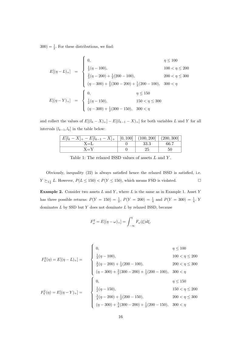
300) = 12 . For these distributions, we find:

E[(η − L)+] =

0, η ≤ 100

13 (η − 100), 100 < η ≤ 200

23 (η − 200) + 1

3 (200− 100), 200 < η ≤ 300

(η − 300) + 23 (300− 200) + 1

3 (200− 100), 300 < η

E[(η − Y )+] =

0, η ≤ 150

12 (η − 150), 150 < η ≤ 300

(η − 300) + 12 (300− 150), 300 < η

and collect the values of E[(lk −X)+] − E[(lk−1 −X)+] for both variables L and Y for all

intervals (lk−1, lk] in the table below:

E[lk −X]+ − E[lk−1 −X]+ [0, 100] (100, 200] (200, 300]X=L 0 33.3 66.7X=Y 0 25 50

Table 1: The relaxed ISSD values of assets L and Y .

Obviously, inequality (22) is always satisfied hence the relaxed ISSD is satisfied, i.e.

Y �1 12L. However, P (L ≤ 150) < P (Y ≤ 150), which means FSD is violated.

Example 2. Consider two assets L and Y , where L is the same as in Example 1. Asset Y

has three possible returns: P (Y = 150) = 12 , P (Y = 200) = 1

4 and P (Y = 300) = 14 . Y

dominates L by SSD but Y does not dominate L by relaxed ISSD, because

F 2ω = E[(η − ω)+] =

∫ η

−∞Fω(ξ)dξ,

F 2L(η) = E[(η − L)+] =

0, η ≤ 100

13 (η − 100), 100 < η ≤ 200

23 (η − 200) + 1

3 (200− 100), 200 < η ≤ 300

(η − 300) + 23 (300− 200) + 1

3 (200− 100), 300 < η

F 2Y (η) = E[(η − Y )+] =

0, η ≤ 150

12 (η − 150), 150 < η ≤ 200

34 (η − 200) + 1

2 (200− 150), 200 < η ≤ 300

(η − 300) + 34 (300− 200) + 1

2 (200− 150), 300 < η

16

illustrating that E[(η − L)+] ≥ E[(η − Y )+], while

E[(300− L)+]− E[(200− L)+] =2003

≤ E[(300− Y )+]− E[(200− Y )+] = 75.

Below we prove one more technical result regarding relaxed ISSD which has important

consequences for a practical way of modelling relaxed ISSD constraints as stated in the rest

of this section.

Proposition 3. Let Y and L be random variables, whose probability distributions are discrete

with realizations y1, · · · , yM and l1, · · · , lK , respectively. Let Y dominate L by relaxed ISSD.

If there exists k ∈ {1, . . . ,K − 1}, such that

{y1, · · · , yM} ∩ (lk, lk+1) = ∅, (30)

then F 1Y (t) ≤ F 1

L(t) for all t ∈ [lk, lk+1]

Proof. For any k such that

{y1, · · · , yM} ∩ (lk, lk+1) = ∅, (31)

F 1Y (t) = F 1

Y (lk), t ∈ [lk, lk+1). Then by the relaxed ISSD relation,

∫ lk+1

lk

F 1Y (t)dt = F 1

Y (lk)(lk+1 − lk) ≤∫ lk+1

lk

F 1L(t)dt = F 1

L(lk)(lk+1 − lk)

⇒ F 1Y (lk) ≤ F 1

L(lk).

Remark 4. By comparing relaxed ISSD and ISSD which is equivalent to FSD, we can see

the relaxation is at the points of ym. Assume the relaxed ISSD is true. From the above

proposition, F 1Y (t) ≤ F 1

L(t) holds in any interval [lk, lk+1) which does not contain any ym.

Actually, even if ym appears in this interval, F 1Y (t) ≤ F 1

L(t) still holds if F 1Y (ym) ≤ F 1

L(lk).

Such a relation is violated only in the interval in which the probability of Y jumps over the

probability of the benchmark L. This violation will not transfer to the next interval because

of relaxed ISSD.

17

Proposition 3 opens a way to express chance constraints in LP form by imposing relaxed

ISSD constraints. Assume L is a benchmark with discrete distribution and the portfolio

Y dominates L by relaxed ISSD, and let lk < lk+1 be two neighbouring realisations of the

benchmark. If [lk, lk+1] is such that the portfolio will not have any realization in this interval,

then

P (Y ≤ t) ≤ P (L ≤ t), ∀t ∈ [lk, lk+1].

Hence, the probability of the portfolio can be constrained for those values in such an interval.

There is an issue of how to guarantee the existence of such intervals. We address this problem

below.

The risk control in ALM modelling reflects concerns about the underfunding which is the

amount of unsatisfied liability. Bogentoft, et al. [3] applied CVaR to control the return of the

pension fund with a certain percentage to cover the liability. While it is difficult and costly

to avoid any underfunding at all, it seems highly desirable to limit the probability that any

underfunding happens. We will show how to express such probability constraints in LP form.

Suppose the portfolio is expected to satisfy the following chance constraint:

P (final wealth− liability < 0) ≤ α, (32)

where α is a given threshold. An interval [θ1, θ2] is assumed to exist such that the following

two equations

final wealth− liability < θ1 (33)

final wealth− liability < θ2 (34)

are equivalent to

final wealth− liability < 0. (35)

For example, it is the same to the fund manager in practice to have either no underfunding

or an underfunding of £1. Then this interval can be [−1, 0]. We assume that such an interval

always exists. Suppose the return of the portfolio is modelled by M scenarios. A benchmark

L can be constructed satisfying the following conditions:

• The benchmark value has K realizations and K > M + 1;

• Among the K realizations, at least M + 1 are allocated in the interval [θ1, θ2], with θ1

and θ2 defined as above; and

18

• Last but most important, P (L− Liability < 0) ≤ α.

If a portfolio outperforms such a benchmark by relaxed ISSD, there must be an interval

[lk, lk+1) ⊂ [θ1, θ2], where the portfolio value has no realization. Then by Proposition 3, this

portfolio has return below lk+1 with probability less than α. While there is no difference to the

fund manager to have an underfunding of lk+1 or 0, the chance constraint of the underfunding

is successfully satisfied. For multiple chance constraints, separate relaxed ISSD constraints

can be applied and the derivation is the same as in the single case.

4 Multi-Stage ALM Model with SSD and Relaxed ISSD

Constraints

Now, we will apply SSD and relaxed ISSD in the multi-stage ALM model to control risk.

Either SSD or relaxed ISSD can be independently incorporated in the model. Both SSD

and relaxed ISSD constraints are set at each stage: overall portfolio returns are required to

dominate a benchmark by SSD and relaxed ISSD constraint guarantees that the portfolio

value minus liabilities dominates a benchmark by relaxed ISSD.

In addition to the notation listed in Section 2, new notation is introduced to construct

the stochastic dominance constraints in the model as follows:

τl: the values of benchmark performance used for the SSD constraint, l = 1, . . . , L;

µk: the values of benchmark performance used for the relaxed ISSD constraint, k = 1, . . . ,K.

These values are set such that the probability of this benchmark being negative is equal to

α, i.e. we want the probability of underfunding to be less than or equal to α;

τl = E[(τl − τ)+], l = 1, . . . , L;

µk = E[(µk − µ)+], k = 1, . . . ,K;

slj,t: shortfall of the portfolio in node j at stage t compared to lth value of the benchmark in

the SSD constraint;

vkj,t: shortfall of the portfolio in node j at stage t compared to kth value of the benchmark

in the relaxed ISSD constraint.

In the following model (36), we can find that (36f) and (36g) are SSD constraints that the

return of the portfolio is restricted to dominate the benchmark τ by SSD; while (36h), (36i)

and (36j) are relaxed ISSD constraints which guarantee that the value of the portfolio minus

the amount of the liability dominates the benchmark µ by relaxed ISSD, so as to control the

19

probability of underfunding:

max∑

j∈NT

πTj (

∑i∈I

(1− γ)WixhTi,j + cTj − λbTj ) (36a)

s.t. (1 + γ)∑i∈I

Wixh0i,0 + c0 = G−A0 +D0 (36b)

(1 + γ)∑i∈I

Wixbti,j + ctj = (1− γ)

∑i∈I

Wixsti,j + (1 +Rt

c,j)ct−1a(j) −At

j +Dtj , (36c)

(1 +Rti,j)xh

t−1i,a(j) + xbti,j − xst

i,j = xhti,j , (36d)

∑i∈I

(1− γ)WixhTi,j + cTj + bTj ≥ ψAT

j , (36e)

∑i∈I

(1 +Rti,j)Wixh

t−1i,a(j) + (1 +Rt

c,j)ct−1a(j) + sl

j,t ≥ τl, (36f)

∑j∈Nt

πtjs

lj,t ≤ τl, l = 1, . . . , L, (36g)

∑i∈I

(1 +Rti,j)Wixh

t−1i,a(j) + (1 +Rt

c,j)ct−1a(j) − ψAj,t + vk

j,t ≥ µk, (36h)

∑j∈Nt

πtjv

kj,t −

∑j∈Nt

πtjv

k−1j,t ≤ µk − µk−1, k = 2, . . . ,K, (36i)

∑j∈Nt

πtjv

1j,t ≤ µ1, (36j)

xhti,j ≥ 0, xst

i,j ≥ 0, xbtj ≥ 0, bTj ≥ 0

xhtj , xst

j , xbtj ∈ Rm

i ∈ I = {1, . . . ,m}, j ∈ Nt = {1, . . . , nt}, t = 1, · · · , T,

l = 1, . . . , L, k = 1, . . . ,K.

Now we can see that, by incorporating SSD in the ALM model, the risk incurred by overall

performance is controlled by requesting that our portfolio outperforms the benchmark by SSD

in (36f) and (36g); by incorporating relaxed ISSD, the risk of underfunding is controlled in

terms of chance constraints (36h), (36i) and (36j).

20

5 Numerical Results

The models discussed in this paper are applicable in practice. We first demonstrate the

advantages of taking stochastic dominance constraints into account using a small example,

followed with an out-of-sample backtest. Then we will show how real-world problems can

be solved. We use the structure-exploiting interior point solver OOPS [20] to solve these

problems and compare its performance with that of the general-purpose commercial optimizer

CPLEX 10.0 on a number of medium scale test examples.

5.1 A Model Example

Consider a small investment problem with 2 stages and 4 stocks to be chosen from. One

stage corresponds to one day. There are 4 branches at the first stage and 2 branches from

each node of the second stage. Both asset returns and liabilities are random. The returns in

per cent of the 4 stocks are shown in Table 2 with the probabilities in brackets and the other

parameters are presented in Table 3:

1st Stg A B C D 2nd Stg A B C D

1 (0.5) 0.0145 -0.1020 -0.0305 0.22991 (0.40) 0.1145 -0.2020 -0.0305 0.02992 (0.10) -0.1060 0.2450 0.0341 0.0167

2 (0.2) 0.0056 0.2050 0.1041 -0.02361 (0.16) 0.1145 -0.2020 -0.0305 0.02992 (0.04) -0.1060 0.2450 0.0341 0.0167

3 (0.2) -0.0113 0.0007 -0.0287 0.16581 (0.16) 0.1145 -0.2020 -0.0305 0.02992 (0.04) -0.1060 0.2450 0.0341 0.0167

4 (0.1) 0.1573 -0.0286 0.0645 -0.07421 (0.08) 0.1145 -0.2020 -0.0305 0.02992 (0.02) -0.1060 0.2450 0.0341 0.0167

Table 2: Returns of the assets in per cent.

Parameter Value# of assets m 4# of leaf nodes nT 8# of SSD benchmarks K1 1# of rISSD benchmarks K2 1length of investment horizon T 2penalty coefficient for underfunding at horizon λ 2lower bound of funding ratio φ 1.01transaction fee ratio γ 0.03

Table 3: Typical parameter values.

We generate the optimal investment strategy using 3 models. In the first one, (i), the

21

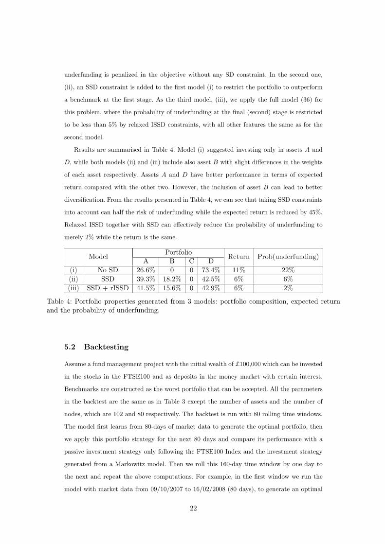
underfunding is penalized in the objective without any SD constraint. In the second one,

(ii), an SSD constraint is added to the first model (i) to restrict the portfolio to outperform

a benchmark at the first stage. As the third model, (iii), we apply the full model (36) for

this problem, where the probability of underfunding at the final (second) stage is restricted

to be less than 5% by relaxed ISSD constraints, with all other features the same as for the

second model.

Results are summarised in Table 4. Model (i) suggested investing only in assets A and

D, while both models (ii) and (iii) include also asset B with slight differences in the weights

of each asset respectively. Assets A and D have better performance in terms of expected

return compared with the other two. However, the inclusion of asset B can lead to better

diversification. From the results presented in Table 4, we can see that taking SSD constraints

into account can half the risk of underfunding while the expected return is reduced by 45%.

Relaxed ISSD together with SSD can effectively reduce the probability of underfunding to

merely 2% while the return is the same.

ModelPortfolio

Return Prob(underfunding)A B C D

(i) No SD 26.6% 0 0 73.4% 11% 22%(ii) SSD 39.3% 18.2% 0 42.5% 6% 6%(iii) SSD + rISSD 41.5% 15.6% 0 42.9% 6% 2%

Table 4: Portfolio properties generated from 3 models: portfolio composition, expected returnand the probability of underfunding.

5.2 Backtesting

Assume a fund management project with the initial wealth of £100,000 which can be invested

in the stocks in the FTSE100 and as deposits in the money market with certain interest.

Benchmarks are constructed as the worst portfolio that can be accepted. All the parameters

in the backtest are the same as in Table 3 except the number of assets and the number of

nodes, which are 102 and 80 respectively. The backtest is run with 80 rolling time windows.

The model first learns from 80-days of market data to generate the optimal portfolio, then

we apply this portfolio strategy for the next 80 days and compare its performance with a

passive investment strategy only following the FTSE100 Index and the investment strategy

generated from a Markowitz model. Then we roll this 160-day time window by one day to

the next and repeat the above computations. For example, in the first window we run the

model with market data from 09/10/2007 to 16/02/2008 (80 days), to generate an optimal

22

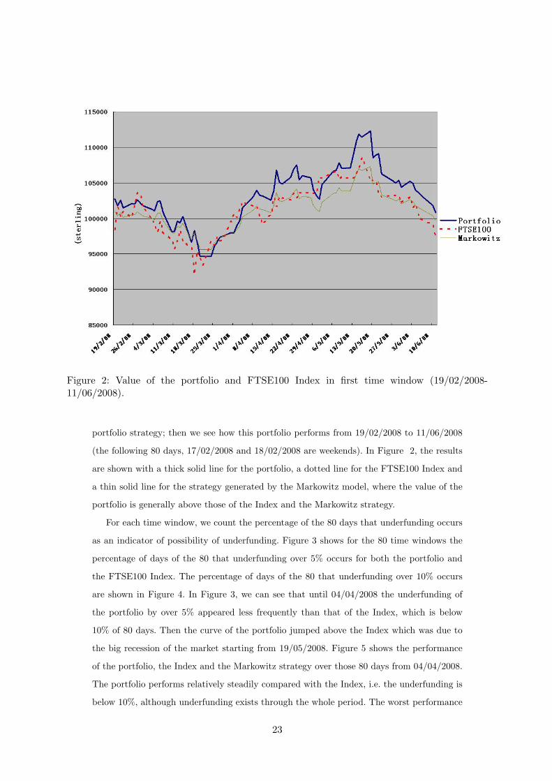
Figure 2: Value of the portfolio and FTSE100 Index in first time window (19/02/2008-11/06/2008).

portfolio strategy; then we see how this portfolio performs from 19/02/2008 to 11/06/2008

(the following 80 days, 17/02/2008 and 18/02/2008 are weekends). In Figure 2, the results

are shown with a thick solid line for the portfolio, a dotted line for the FTSE100 Index and

a thin solid line for the strategy generated by the Markowitz model, where the value of the

portfolio is generally above those of the Index and the Markowitz strategy.

For each time window, we count the percentage of the 80 days that underfunding occurs

as an indicator of possibility of underfunding. Figure 3 shows for the 80 time windows the

percentage of days of the 80 that underfunding over 5% occurs for both the portfolio and

the FTSE100 Index. The percentage of days of the 80 that underfunding over 10% occurs

are shown in Figure 4. In Figure 3, we can see that until 04/04/2008 the underfunding of

the portfolio by over 5% appeared less frequently than that of the Index, which is below

10% of 80 days. Then the curve of the portfolio jumped above the Index which was due to

the big recession of the market starting from 19/05/2008. Figure 5 shows the performance

of the portfolio, the Index and the Markowitz strategy over those 80 days from 04/04/2008.

The portfolio performs relatively steadily compared with the Index, i.e. the underfunding is

below 10%, although underfunding exists through the whole period. The worst performance

23

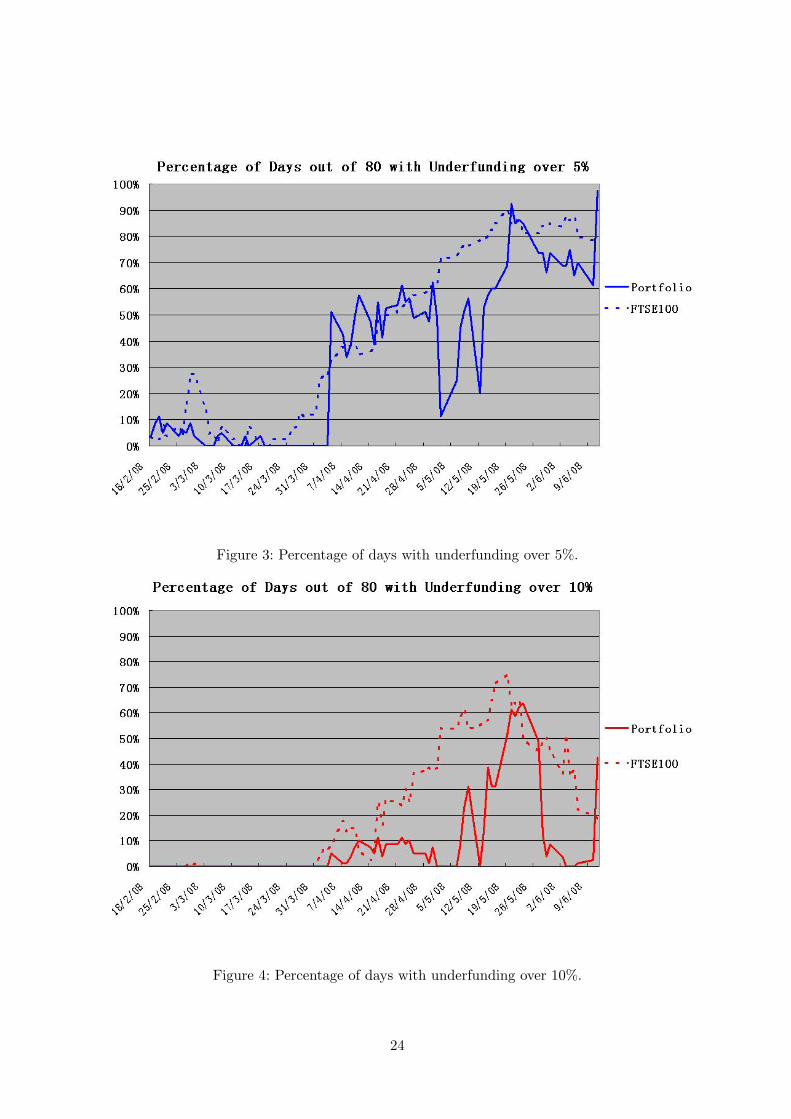
Figure 3: Percentage of days with underfunding over 5%.

Figure 4: Percentage of days with underfunding over 10%.

24

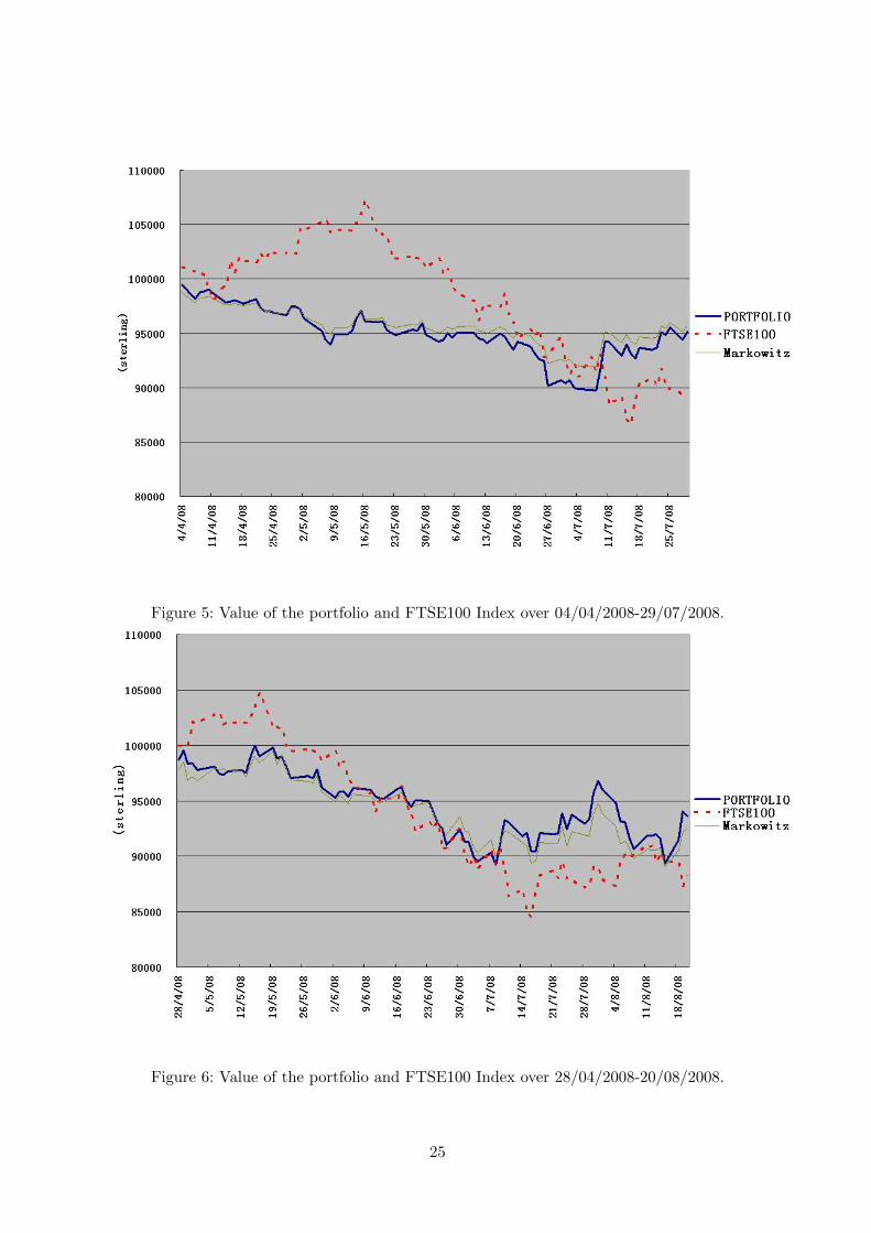
Figure 5: Value of the portfolio and FTSE100 Index over 04/04/2008-29/07/2008.

Figure 6: Value of the portfolio and FTSE100 Index over 28/04/2008-20/08/2008.

25

of the portfolio in both Figures 3 and 4 appears around 20/05/2008, similarly to the Index,

when the market was at a turning point and started to decrease along the way until touching

a 21-month-low on 15/07/2008.

Through the whole test the portfolio generated by the model presents a relative steady

performance compared with FTSE100 Index. For example on 28/04/2008, the two curves

in Figure 3 cross, which means the percentages of days with underfunding over 5% are

the same for both the portfolio and the Index investment. However, the possibility of the

portfolio underfunding over 10% corresponding to that day is 5% as shown in Figure 4,

significantly smaller than the 37.5% of the Index. That 80-day performance is illustrated in

Figure 6. Among the 80 time windows, there are 58 windows (72.5%) when the percentage

of days with portfolio underfunding over 5% is smaller than that of the Index, as illustrated

in Figure 3, and 75 windows (93.75%) for underfunding over 10%, as is shown in Figure 4.

5.3 Numerical Efficiency

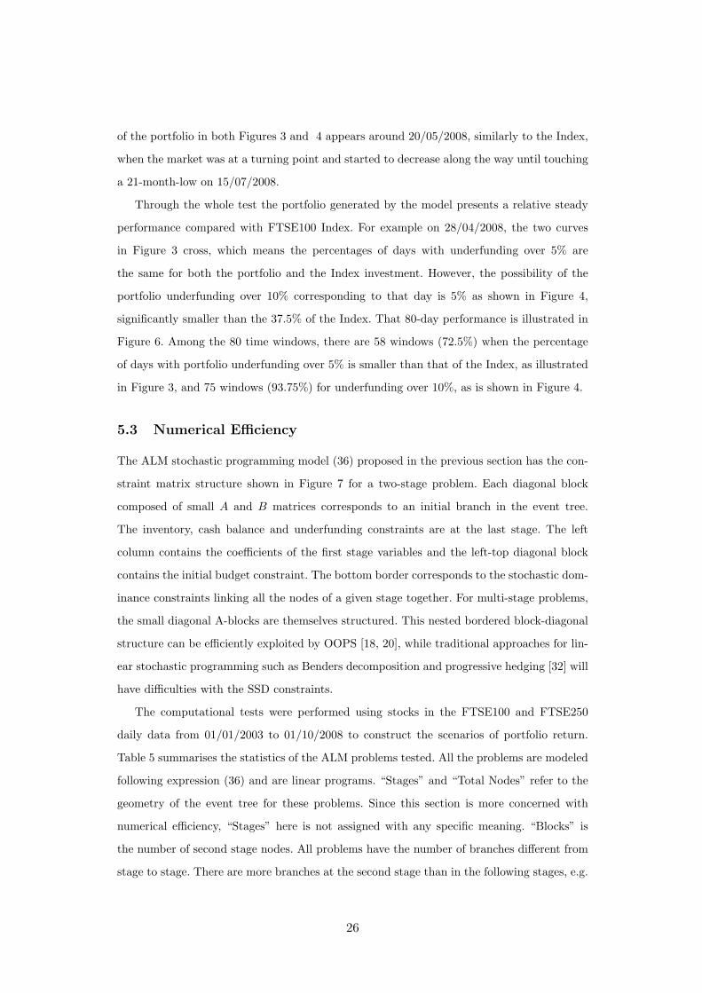
The ALM stochastic programming model (36) proposed in the previous section has the con-

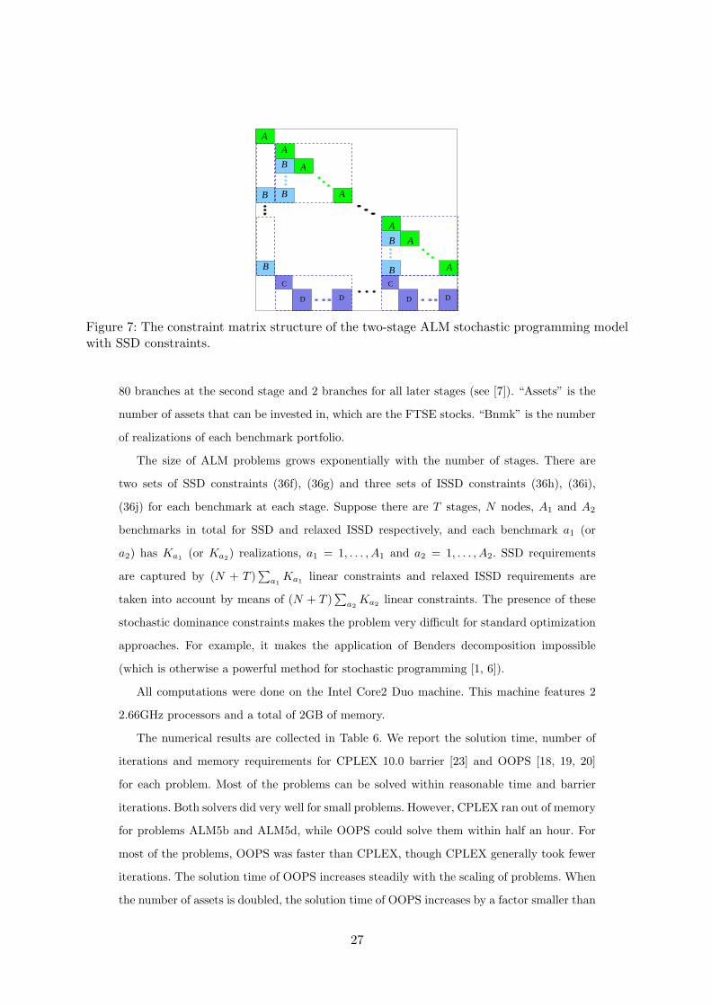
straint matrix structure shown in Figure 7 for a two-stage problem. Each diagonal block

composed of small A and B matrices corresponds to an initial branch in the event tree.

The inventory, cash balance and underfunding constraints are at the last stage. The left

column contains the coefficients of the first stage variables and the left-top diagonal block

contains the initial budget constraint. The bottom border corresponds to the stochastic dom-

inance constraints linking all the nodes of a given stage together. For multi-stage problems,

the small diagonal A-blocks are themselves structured. This nested bordered block-diagonal

structure can be efficiently exploited by OOPS [18, 20], while traditional approaches for lin-

ear stochastic programming such as Benders decomposition and progressive hedging [32] will

have difficulties with the SSD constraints.

The computational tests were performed using stocks in the FTSE100 and FTSE250

daily data from 01/01/2003 to 01/10/2008 to construct the scenarios of portfolio return.

Table 5 summarises the statistics of the ALM problems tested. All the problems are modeled

following expression (36) and are linear programs. “Stages” and “Total Nodes” refer to the

geometry of the event tree for these problems. Since this section is more concerned with

numerical efficiency, “Stages” here is not assigned with any specific meaning. “Blocks” is

the number of second stage nodes. All problems have the number of branches different from

stage to stage. There are more branches at the second stage than in the following stages, e.g.

26

C

DD

C

DD

B

B

A

A

B

B

A

A

A

AB

B

A

Figure 7: The constraint matrix structure of the two-stage ALM stochastic programming modelwith SSD constraints.

80 branches at the second stage and 2 branches for all later stages (see [7]). “Assets” is the

number of assets that can be invested in, which are the FTSE stocks. “Bnmk” is the number

of realizations of each benchmark portfolio.

The size of ALM problems grows exponentially with the number of stages. There are

two sets of SSD constraints (36f), (36g) and three sets of ISSD constraints (36h), (36i),

(36j) for each benchmark at each stage. Suppose there are T stages, N nodes, A1 and A2

benchmarks in total for SSD and relaxed ISSD respectively, and each benchmark a1 (or

a2) has Ka1 (or Ka2) realizations, a1 = 1, . . . , A1 and a2 = 1, . . . , A2. SSD requirements

are captured by (N + T )∑

a1Ka1 linear constraints and relaxed ISSD requirements are

taken into account by means of (N + T )∑

a2Ka2 linear constraints. The presence of these

stochastic dominance constraints makes the problem very difficult for standard optimization

approaches. For example, it makes the application of Benders decomposition impossible

(which is otherwise a powerful method for stochastic programming [1, 6]).

All computations were done on the Intel Core2 Duo machine. This machine features 2

2.66GHz processors and a total of 2GB of memory.

The numerical results are collected in Table 6. We report the solution time, number of

iterations and memory requirements for CPLEX 10.0 barrier [23] and OOPS [18, 19, 20]

for each problem. Most of the problems can be solved within reasonable time and barrier

iterations. Both solvers did very well for small problems. However, CPLEX ran out of memory

for problems ALM5b and ALM5d, while OOPS could solve them within half an hour. For

most of the problems, OOPS was faster than CPLEX, though CPLEX generally took fewer

iterations. The solution time of OOPS increases steadily with the scaling of problems. When

the number of assets is doubled, the solution time of OOPS increases by a factor smaller than

27

Problem Stages Blocks Assets Bnmk Total Nodes Constraints VariablesT B I L |N | =

∑T−1t=0 Nt (I+L+2)|N| (3I+L+2)|N|

ALM1a 2 80 64 20 81 6966 17334ALM1b 2 40 128 20 41 6150 16646ALM1c 2 80 128 20 81 12150 32886ALM1d 2 160 128 20 161 24150 65366ALM2a 2 80 64 40 81 8586 18954ALM2b 2 40 128 40 41 6970 17466ALM2c 2 80 128 40 81 13770 34506ALM2d 2 160 128 40 161 27370 68586ALM3a 2 80 64 80 81 11826 22194ALM3b 2 40 128 80 41 8610 19106ALM3c 2 80 128 80 81 17010 37746ALM3d 2 160 128 80 161 33810 75026ALM4a 3 40 128 10 201 28140 79596ALM4b 3 80 128 10 241 33740 95436ALM5a 4 40 128 10 1641 229740 649836ALM5b 4 40 128 10 2921 408940 1156716ALM5c 4 80 128 10 1681 235340 665676ALM5d 4 80 128 10 3281 459340 1299276

Table 5: Problems scales for comparison of OOPS with CPLEX.

three, which can be seen from the comparison of solution statistics of ALM1a and ALM1c,

ALM2a and ALM2c, ALM3a and ALM3c. By comparing solution statistics of problems

ALM1a, ALM2a and ALM3a, we can observe the influence of the number of benchmark

realizations on the efficiency of both solvers compared. The solution statistics of ALM1b/c/d,

ALM2b/c/d and ALM3b/c/d demonstrate that the solution time of CPLEX increases with

the number of blocks much faster than that of OOPS. Both CPLEX and OOPS solution times

are badly affected by the increase of the number of benchmark realizations. The memory

requirements of OOPS are generally smaller than those of CPLEX.

6 Conclusions

In addition to the operational constraints, i.e. inventory and cash balance, ALM models

require sophisticated risk control to ensure that liabilities are met. As a consequence, un-

derfunding, which measures the amount of non-satisfied liabilities, is expected to be zero.

Stochastic dominance as a reference to efficient risk control can manage the risk in ALM

problems effectively by its consistency with utility theory. Furthermore, the concept of re-

laxed interval second-order stochastic dominance is developed and used to model chance

28

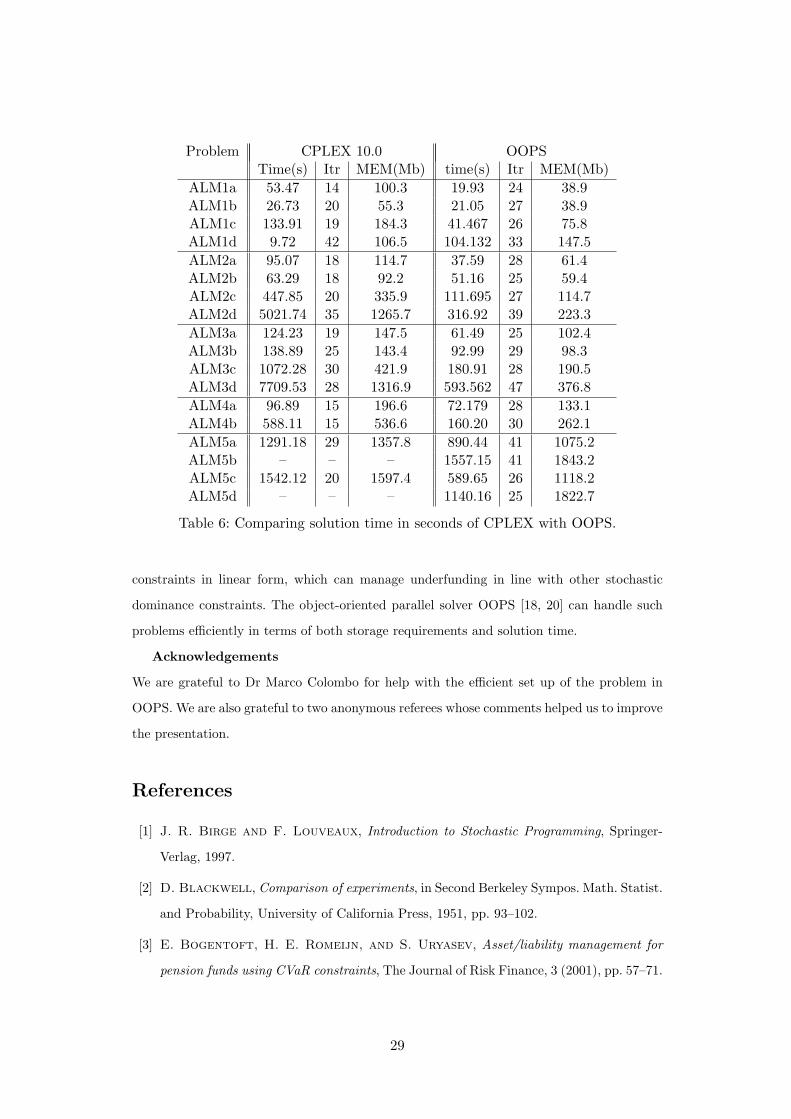
Problem CPLEX 10.0 OOPSTime(s) Itr MEM(Mb) time(s) Itr MEM(Mb)

ALM1a 53.47 14 100.3 19.93 24 38.9ALM1b 26.73 20 55.3 21.05 27 38.9ALM1c 133.91 19 184.3 41.467 26 75.8ALM1d 9.72 42 106.5 104.132 33 147.5ALM2a 95.07 18 114.7 37.59 28 61.4ALM2b 63.29 18 92.2 51.16 25 59.4ALM2c 447.85 20 335.9 111.695 27 114.7ALM2d 5021.74 35 1265.7 316.92 39 223.3ALM3a 124.23 19 147.5 61.49 25 102.4ALM3b 138.89 25 143.4 92.99 29 98.3ALM3c 1072.28 30 421.9 180.91 28 190.5ALM3d 7709.53 28 1316.9 593.562 47 376.8ALM4a 96.89 15 196.6 72.179 28 133.1ALM4b 588.11 15 536.6 160.20 30 262.1ALM5a 1291.18 29 1357.8 890.44 41 1075.2ALM5b – – – 1557.15 41 1843.2ALM5c 1542.12 20 1597.4 589.65 26 1118.2ALM5d – – – 1140.16 25 1822.7

Table 6: Comparing solution time in seconds of CPLEX with OOPS.

constraints in linear form, which can manage underfunding in line with other stochastic

dominance constraints. The object-oriented parallel solver OOPS [18, 20] can handle such

problems efficiently in terms of both storage requirements and solution time.

Acknowledgements

We are grateful to Dr Marco Colombo for help with the efficient set up of the problem in

OOPS. We are also grateful to two anonymous referees whose comments helped us to improve

the presentation.

References

[1] J. R. Birge and F. Louveaux, Introduction to Stochastic Programming, Springer-

Verlag, 1997.

[2] D. Blackwell, Comparison of experiments, in Second Berkeley Sympos. Math. Statist.

and Probability, University of California Press, 1951, pp. 93–102.

[3] E. Bogentoft, H. E. Romeijn, and S. Uryasev, Asset/liability management for

pension funds using CVaR constraints, The Journal of Risk Finance, 3 (2001), pp. 57–71.

29

[4] D. R. Carino, T. Kent, D. H.Myers, C. Stacy, M. Sylvanus, A. L. Turner,

K. Watanabe, and W. T. Ziemba, The Russell-Yasuda Kasai model: An as-

set/liability model for a Japanese insurance company using multistage stochastic pro-

gramming, Interfaces, 24 (1994), pp. 29–49.

[5] D. R. Carino and W. T. Ziemba, Formulation of the Russell-Yasuda Kasai financial

model, Operations Research, 46 (1998), pp. 433–449.

[6] G. Consigli and M. A. H. Dempster, Dynamic stochastic programming for asset-

liability management, Annals of Operation Research, 81 (1998), pp. 131–161.

[7] M. A. Dempster, M. Germano, E. A. Medova, M. I. Rietbergen, F. Sandrini,

and M. Scrownston, Designing minimum guaranteed return funds, Quantitative Fi-

nance, 7 (2007), pp. 245–256.

[8] D. Dentcheva, R. Henrion, and A. Ruszczynski, Stability and sensitivity of op-

timization problems with first order stochastic dominance constraints, SIAM Journal of

Optimization, 18 (2007), pp. 322–337.

[9] D. Dentcheva and A. Ruszczynski, Optimization with stochastic dominance con-

straints, SIAM Journal of Optimization, 14 (2003), pp. 548–566.

[10] , Optimality and duality theory for stochastic optimization problems with nonlinear

dominance constraints, Mathematical Programming, 99 (2004), pp. 329–350.

[11] , Portfolio optimization with stochastic dominance constraints, Journal of Banking

Finance, 30 (2006), pp. 433–451.

[12] , Optimization with multivariate stochastic dominance constraints, Mathematical

Programming, 117 (2009), pp. 111–127.

[13] C. I. Fabian, G. Mitra, and D. Roman, Processing second-order stochastic dom-

inance models using cutting-plane representations, Mathematical Programming. DOI:

10.1007/s10107-009-0326-1.

[14] C. I. Fabian and A. Veszpremi, Algorithms for handling CVaR constraints in dy-

namic stochastic programming models with applications to finance, Journal of Risk, 10

(2008), pp. 111–131.

[15] R. Gollmer, U. Gotzes, F. Neise, and R. Schultz, Risk modeling via stochastic

dominance in power systems with dispersed generation, tech. report, Department of

Mathematics, University of Duisburg-Essen, 2007.

30

[16] R. Gollmer, U. Gotzes, and R. Schultz, A note on second-order stochastic domi-

nance constraints induced by mixed-integer linear recourse, Mathematical Programming,

(2009). Published online Febrary 2009.

[17] R. Gollmer, F. Neise, and R. Schultz, Stochastic programs with first-order domi-

nance constraints induced by mixed-integer linear recourse, SIAM Journal on Optimiza-

tion, 19 (2008), pp. 552–571.

[18] J. Gondzio and A. Grothey, Parallel interior point solver for structured quadratic

programs: Application to financial planning problems, Annals of OR, 152 (2007),

pp. 319–339.

[19] J. Gondzio and A. Grothey, Solving nonlinear portfolio optimization problems with

the primal-dual interior point method, European Journal of Operational Research, 181

(2007), pp. 1019–1029.

[20] J. Gondzio and A. Grothey, Exploiting structure in parallel implementation of in-

terior point methods for optimization, Computational Management Science, 6 (2009),

pp. 135–160.

[21] J. Hadar and W. R. Russell, Rules for ordering uncertain prospects, Amer. Eco-

nomic Rev., 59 (1969), pp. 25–34.

[22] G. Hanoch and H. Levy, The efficiency analysis of choices involving risk, Rev. Eco-

nomics Studies, 36 (1969), pp. 335–346.

[23] ILOG, Ilog cplex 10.0. www.ilog.com.

[24] P. Kall and S. W. Wallace, Stochastic Programming, John Wiley & Sons, 1994.

[25] P. Krokhmal, J. Palmquist, and S. Uryasev, Portfolio optimization with condi-

tional value-at-risk objective and constraints, Journal of Risk, 4 (2001), pp. 43–68.

[26] M. I. Kusy and W. T. Ziemba, A bank asset and liability management model, Oper-

ations Research, 34 (1986), pp. 356–376.

[27] H. Levy, Stochastic dominance and expected utility: survey and analysis, Management

Science, 38 (1992), pp. 555–593.

[28] H. M.Markowitz, Portfolio Selection, Efficient Diversification of Investments, John

Wiley& Sons, 1959.

[29] N. Noyan, G. Rudolf, and A. Ruszczynski, Relaxations of linear programming

problems with first order stochastic dominance constraints, Operations Research Letters,

34 (2006), pp. 653–659.

31

[30] W. Ogryczak and A. Ruszczynski, Dual stochastic dominance and related mean-risk

models, SIAM Journal of Optimization, 13 (2002), pp. 60–78.

[31] D. H. Pyle, On the theory of financial intermediation, Journal of Finance, 26 (1971),

pp. 737–747.

[32] R. T. Rockafellar and R. J.-B. Wets, Scenarios and policy aggregation in opti-

mization under uncertainty, Mathematics of Operations Research, 16 (1991), pp. 119–

147.

[33] D. Roman, K. Darby-Dowman, and G. Mitra, Portfolio construction based on

stochastic dominance and target return distributions, Mathematical Programming, 108

(2006), pp. 541–569.

[34] A. Ruszczynski and A. Shapiro, Optimization of convex risk functions, Mathematics

of Operation Research, 31 (2006), pp. 433–452.

[35] A. Ruszczynski and R. J. Vanderbei, Frontiers of stochastic nondominated portfo-

lios, Econometrica, 71 (2003), pp. 1287–1297.

[36] W. T. Ziemba and J. M. Mulvey, Worldwide Asset and Liability Modeling, Publi-

cations of the Newton Institute, Cambridge University Press, Cambridge, 1998.

32