assimilation of simulated doppler radar observations with...

AUGUST 2003 1663S N Y D E R A N D Z H A N G

q 2003 American Meteorological Society

Assimilation of Simulated Doppler Radar Observations with anEnsemble Kalman Filter*

CHRIS SNYDER

National Center for Atmospheric Research, Boulder, Colorado

FUQING ZHANG

Department of Atmospheric Science, Texas A&M University, College Station, Texas

(Manuscript received 11 November 2002, in final form 30 January 2003)

ABSTRACT

Assimilation of Doppler radar data into cloud models is an important obstacle to routine numerical weatherprediction for convective-scale motions; the difficulty lies in initializing fields of wind, temperature, moisture,and condensate given only observations of radial velocity and reflectivity from the radar. This paper investigatesthe potential of the ensemble Kalman filter (EnKF), which estimates the covariances between observed variablesand the state through an ensemble of forecasts, to assimilate radar observations at convective scales. In the basicexperiment, simulated observations are extracted from a reference simulation of a splitting supercell and assim-ilated using the EnKF and the same numerical model that produced the reference simulation. The EnKF producesaccurate analyses, including the unobserved variables, after roughly 30 min (or six scans) of radial velocityobservations. Additional experiments, in which forecasts are made from the ensemble-mean analysis, reveal thatforecast errors grow significantly in this simple system, so that the ability of the EnKF to track the referencesolution is not simply because of stable system dynamics. It is also found that the covariances between radialvelocity and temperature, moisture, and condensate are important to the quality of the analyses, as is theinitialization chosen for the ensemble members prior to assimilating the first observations. These results arepromising, especially given the ease of implementing the EnKF. A number of important issues remain, however,including the initialization of the ensemble prior to the first observation, the treatment of uncertainty in theenvironmental sounding, the role of error in the forecast model (particularly the microphysical parameterizations),and the treatment of lateral boundary conditions.

1. Introduction

A long-standing problem in meteorology is to esti-mate, or retrieve, the state of the atmosphere in somedomain given observations of reflectivity and radial ve-locity from one or more Doppler radars. (Alternatively,one may speak of assimilating these observations.) Do-ing this requires an algorithm that infers from the ob-servations those variables not directly observed, suchas vertical velocity and temperature, and this in turnrequires additional information beyond the observationsthemselves. Such information is available, in principle,from our knowledge of the governing equations, andvarious techniques have been devised to utilize the gov-erning equations in assimilation or retrieval.

* The National Center for Atmospheric Research is sponsored bythe National Science Foundation.

Corresponding author address: Dr. C. Snyder, NCAR, P.O. Box3000, Boulder, CO 80307-3000.E-mail: [email protected]

This paper explores for the first time the use of anensemble Kalman filter (EnKF) to assimilate single-Doppler radar observations in a cloud-scale model. TheEnKF is a novel and flexible technique for data assim-ilation, first proposed in the geophysical literature byEvensen [1994; but see also Leith (1983, 375–377)].The EnKF uses forecast covariances between observedand unobserved variables to spread information fromthe observations both spatially and between variables.These covariances are estimated from an ensemble ofprior forecasts initialized when observations were lastavailable. Section 2 provides further background on theEnKF.

Other approaches for analyzing the atmospheric stategiven radar observations fall into two categories: re-trieval algorithms and four-dimensional variational as-similation (4DVAR). Retrieval algorithms typically be-gin by estimating the wind field given observations ofradial velocity from one or more radars. Since onlycertain components of the velocity are observed, theentire velocity field is estimated using additional infor-mation or constraints (such as continuity, the prognostic

1664 VOLUME 131M O N T H L Y W E A T H E R R E V I E W

equation for radial velocity, or the evolution of the re-flectivity field). Given knowledge of the wind field, thethermodynamic variables are then estimated from thevertical momentum equation after first calculating pres-sure perturbations at each level from the horizontal mo-mentum equations. Recent results from different algo-rithms, as well as earlier references, can be found in Xuet al. (2001), Montmerle et al. (2001), and Weygandt etal. (2002).

Four-dimensional variational schemes seek to fit anumerical simulation to observations spread over a timeinterval by adjusting the state at the beginning of theinterval. Like retrieval algorithms, 4DVAR has shownpractical value in estimating unobserved variables givenradar observations (Sun and Crook 1997, 1998). Unlikethe more empirical retrieval algorithms, however,4DVAR analyzes all variables in a unified fashion.4DVAR also allows the systematic treatment of obser-vation error and information from recent forecasts, butcovariance matrices for both the observation and fore-cast error must be specified. Further background on4DVAR appears in Sun and Crook (1997), while Rabieret al. (2000) discuss the implementation of 4DVAR foran advanced numerical weather prediction model.

The EnKF has several appealing properties that mo-tivate its consideration as an alternative to retrieval al-gorithms or 4DVAR. Like 4DVAR, it is a statisticalscheme that handles uncertainty in the observations andthe prior forecast gracefully and approximates, subjectto certain assumptions, the Bayesian update for the fore-cast state given new observations. The EnKF also pro-vides direct estimates of the forecast covariances fromthe forecast ensemble and then explicitly updates thatensemble to be consistent with the uncertainty of theanalysis. Thus, because it produces not only an analysis(the ensemble mean) but also an ensemble of initialconditions, the EnKF is a natural foundation for ensem-ble forecasting schemes. This is particularly importantat convective scales, where probabilistic forecasts maybe warranted even at lead times of an hour. Finally, theEnKF is both relatively simple to implement, as tangentlinear and adjoint versions of the forecast model are notrequired, and relatively straightforward to parallelize.

While applications of the EnKF to large-scale flowshave progressed nearly to the point of operational testing(Mitchell et al. 2002; further references appear in section2), similar successes are not guaranteed at convectivescales, where the motions are fully three dimensional,are driven by distinctly nonlinear microphysical pro-cesses, and lack the approximate balances between themass and wind fields, such as geostrophy, that pertainat larger scales. In order to test the EnKF at convectivescales and with radar observations, we extract simulatedradial-velocity observations from a numerical simula-tion of a splitting supercell and then use the EnKF toassimilate those observations. A detailed description ofthe numerical experiments appears in section 3.

The results of these experiments show that the EnKF

has strong potential for convective-scale assimilation;specifically, the state of the simulated supercell can beaccurately estimated given an initial sounding for thedomain and several volume scans of radial velocity.Section 4 presents these results, together with some dis-cussion of the characteristics of the forecast covariances.Since supercells are robust solutions, in the sense thata variety of initial conditions can and will produce qual-itatively similar supercells given an appropriate envi-ronmental sounding, one might worry that predictionand data assimilation for a system of supercells areanomalously easy. We show in section 5 that forecasterrors in fact grow significantly even in our idealizedsystem. Section 6 addresses tuning the filter, the im-portance of the cross covariances between radial veloc-ity and temperature or moisture or rainwater, and therole of the initialization of the ensemble. We summarizein the final section and outline a number of interestingissues that are not addressed in this initial study.

2. The ensemble Kalman filter

This section provides further background on the en-semble Kalman filter. We begin with a heuristic look atthe central ideas in section 2a, then informally reviewthe Kalman filter (section 2b), and finally detail thespecific ensemble technique employed here (section 2c).Readers familiar with the EnKF may wish to skip di-rectly to section 3, while those interested in a morecomplete and rigorous introduction to estimation theoryand the Kalman filter are referred to Cohn (1997). Fur-ther discussion of aspects of the EnKF, together withresults for large scales in the atmosphere, can be foundin Houtekamer and Mitchell (1998), Hamill and Snyder(2000), Anderson (2001), Whitaker and Hamill (2002),and Mitchell et al. (2002). There is also a substantialoceanic literature; see Brusdal et al. (2003), Keppenneand Rienecker (2002), and references therein.

Except for the dimensions of the state and observationvectors, our notation will follow that of Ide et al. (1997).

a. Basic notions

Suppose that at some time, t 5 tk, and over someregion of interest, we possess an ensemble of forecaststhat are representative, in a sense to be made more pre-cise below, of the forecast uncertainty. Typically, theensemble-mean forecast is the best prediction of theatmospheric state at tk. Now suppose we receive anobservation valid at the same time tk. Our problem isthen to assimilate the observation or equivalently toupdate our prediction of the state and its uncertaintygiven this new observation. While the observation ob-viously carries information about the measured quantity,we wish also to extract information about the unob-served portion of the state. How can this be done?

Figure 1a portrays the situation schematically. Fordefiniteness, suppose that the observation is of radial


FIG. 1. Schematic depiction of the EnKF update (or analysis). (a) Forecast values of w andy r for an ensemble of 50 members (black dots). Thin arrows on each axis show the ensemblemeans, each roughly 9 m s21. A hypothetical observation of y r equal to 14 m s21 is indicatedby the bold arrow on the y r axis, while the accompanying curve is meant to suggest theobservational uncertainty. (b) As in Fig. 1a but for the updated ensemble given the observationof y r. The forecast ensemble and observation are reproduced in gray for reference.

velocity y r at some location and the unobserved variableis vertical velocity w at another location. The forecastsfrom each ensemble member for y r and w are shown asa scatterplot; in this case, the sample of ensemble mem-bers suggests that y r and w are positively correlated inthe forecast. Our best forecasts of each variable, theensemble means, are indicated on each axis by the thinarrows. The observed value of y r is assumed to be 14m s21 and is marked on the vertical axis by a thickarrow, along with the specified observational error dis-tribution.

Intuitively, we expect that the best estimate for y r

should lie between the observed value and the meanforecast, and that the uncertainty in this updated, orposterior, estimate should be smaller than that of eitherthe observation or the forecast. In addition, it is clearthat refining our estimate of y r provides information onw; the updated estimate of w should increase, since y r

and w were positively correlated in the forecast and theobservation indicated that y r was larger than was fore-casted.

The updated situation given the observation is shownschematically in Fig. 1b. The updated ensemble is againdisplayed as a scatterplot and the updated means indi-cated by arrows on each axis, while the forecast andobserved quantities from Fig. 1a are shown in gray. Asintuition suggested, the updated ensemble has lessspread in both variables, reflecting the additional in-formation provided by the observation; the updated es-timate of y r lies between the forecast mean and theobservation; and the mean of w has increased from theforecast value. The EnKF, which provided the updatedensemble in Fig. 1b, will be discussed below after abrief review of the Kalman filter.

b. The Kalman filter

Let x of dimension Nx be the state of the system insome discrete representation, such as values on a regulargrid. Thus, x consists of all gridpoint values for allvariables concatenated into a single vector of length Nx.For the purposes of this paper, we will ignore the oftenprickly issues that surround projecting the continuousatmosphere onto a discrete representation and account-ing for the uncertainties associated with that projection(see Cohn 1997).

Since we have a limited set of imperfect observations,the true state of the system, denoted by xt, cannot bedetermined precisely. It is therefore convenient to con-sider xt to be a random variable; the most that can beknown about the system is then p(xt), the probabilitydistribution function (pdf ) of xt. Our goal becomes toestimate and forecast p(xt) given the available obser-vations.

Now suppose, as in the section above, that we havemade a forecast of p(xt) at a time to and possess a setor vector yo of Ny observations also valid at to.1 Subjectto two assumptions, the Kalman filter provides formulasfor calculating p(xt | yo), the pdf of xt given the obser-vations yo. The first assumption is that the observationsare linearly related to xt:

ty 5 Hx 1 e, (1)

where H is a Ny 3 Nx matrix mapping the state variables

1 To be more precise, p(xt) is the pdf for xt at t 5 to conditionedon all observations prior to yo; this is why we refer to p(xt(t 5 to)as a forecast. Since all the equations in this section are valid at t 5to and p(xt) is always conditioned on the prior observations, we willsuppress explicit references to to or the observations prior to to.


onto the observations, and e is a random error vectorof dimension Ny that is independent of xt. The secondassumption is that both the prior (or background) fore-cast of p(xt) and the pdf of e are Gaussian, where theforecast has mean f and covariance Pf and the obser-xvation error has zero mean and covariance R.

Under these assumptions, p(xt | yo) is also Gaussian,with mean a and covariance Pa given by the Kalmanxfilter analysis equations,

a f o fx 5 x 1 K(y 2 Hx ), (2a)a fP 5 (I 2 KH)P , (2b)

where

T 21f T fK 5 P H (HP H 1 R) . (3)

In order to assimilate subsequent observations, a methodis also required to predict the forecast covariances atlater times given Pa; we will discuss the covariancepropagation used in the EnKF in section 2c below. Since

T t t T t tfP H [ Cov(x , x )H 5 Cov(x , Hx ),

P f HT is the forecasted covariance of the state and ob-served variables. We will define 5 P fHT to reflectfPxy

this.Interpretation of (2) is simplest for a single, scalar

observation yo. In that case, is a column vector c offPxy

dimension Nx, HP f HT 1 R is a scalar d, and the updateof the ith element of the mean becomes

a f fox 5 x 1 c (y 2 Hx )/d.i i i (4a)

This result corresponds heuristically to Fig. 1 (settingxi to be the vertical velocity and y to be the radial ve-locity): the updated estimate differs from the priorax i

estimate by an amount proportional to the product offx i

yo 2 H f and ci 5 Cov( , Hxt). For example, if the ob-tx xi

servation yo is greater than its forecast value H f and ifxis positively correlated with Hxt (ci . 0), then the an-txi

alyzed estimate should be greater than the forecast .a fx xi i

The update of the covariance matrix also simplifiesfor a single observation, with (2b) becoming

Ta fP 5 P 2 cc /d. (4b)

If we think of the forecast uncertainty of a state variableas being measured by its variance (the correspondingdiagonal element of P f ), then the observation reducesthe uncertainty most in state variables that have largecovariance with the observed quantity.

We will use one further property of the Kalman filterto simplify the implementation of the EnKF below. Ifthe observations (1) have independent errors, then theupdate (2), which treats all observations (i.e., each el-ement of y) simultaneously, is equivalent to serial as-similation of individual observations through repeatedapplication of (4). To be more precise, one can assim-ilate the first element of yo using (4) and then assim-oy1

ilate subsequent again using (4) but with P f replacedoyj

in the definition of c by the Pa calculated for , oroyj21

equivalently using the expectation conditioned on ,oy1

. . . , to calculate 5 Cov(xt, Hxt). We emphasizeo fy Pxyj21

that independent observation errors and serial assimi-lation of observations are not required for the EnKF butdo result in a simpler algorithm.

Finally, it is important to emphasize that the Kalmanfilter update is optimal only in the case of linear ob-servation operators and Gaussian errors [see (1) and theassociated discussion]. Convective-scale dynamics,however, are often nonlinear, in part because of the im-portance of latent heat release and other microphysicalprocesses. Thus, forecast pdfs will potentially be non-Gaussian and the Kalman filter update will at best ap-proximate the mean and covariance of p(xt | yo).

c. The algorithm

As discussed above, the Kalman filter is a scheme forupdating p(xt) given observations yo. The idea under-lying ensemble filtering techniques is to work with asample, or ensemble, drawn from p(xt) rather than withp(xt) itself. This notion was first proposed for data as-similation in the geophysical literature by Evensen(1994) but is of course at the heart of ensemble fore-casting as well.

The algorithm proceeds in two steps, an analysis orupdate step and a forecast or propagation step, both ofwhich are described in detail below. The analysis stepbegins with an ensemble drawn from p(xt) and convertsthis ensemble into a sample from the updated distri-bution p(xt | yo) conditioned on the most recent obser-vations yo. The analysis proceeds according to the Kal-man filter equations (2)–(4) but with the required meansand covariances replaced by the sample values

Ne

f 21 fx 5 N x , (5)Oe nn51

Ne

21 f f f f TfP 5 (N 2 1) (x 2 x )(Hx 2 Hx ) . (6)Oxy e n nn51

In the forecast step, forecasts are made from each en-semble member produced in the analysis step; this is aMonte Carlo approximation to propagating the p(xt | yo)forward to the time of the next observation. (Imperfec-tions of the forecast model should also be accounted forin this step, although this issue will not arise in thepresent experiments.) The forecast ensemble is thenused in the next analysis step and the algorithm contin-ues.

As an aside, we note that this algorithm unifies en-semble forecasting and data assimilation. The ensembleof forecasts provides the statistical information, requiredfor data assimilation, concerning the uncertainty at agiven time and location and the relations between ob-servations and state variables. The analysis step, in turn,explicitly constructs an appropriate analysis ensembleto serve as initial conditions for subsequent forecasts.


1) THE ANALYSIS STEP

In the analysis step, observations are processed se-rially, as described above. For each observation, thealgorithm first calculates the mean of the prior ensemblefrom (5) and the difference of each member from themean. The ensemble mean is then updated according to(4a), but replacing ci and d with sample covariancescalculated from the ensemble.

In addition to updating the ensemble mean, thescheme must also update the difference of each memberfrom the mean, which corresponds to the covarianceupdate (2b) of the Kalman filter. Following Whitakerand Hamill (2002), the update of the nth member fromthe mean is given by

a a f fx 2 x 5 [I 2 b(c/d)H](x 2 x ),n n (7)

where b 5 [1 1 (R/d)1/2]21, and c and d are sampleestimates, as in (5) and (6), of c and d defined prior to(4). [See Anderson (2001) for a different, but mathe-matically equivalent, version of (7).] The ensemble{ } calculated in (7) then becomes the prior ensembleaxn

for the assimilation of the next observation and the al-gorithm continues until all observations are processed.

In practice, the update is restricted to those state var-iables that are within a certain radius from the obser-vation location. We do this because state variables farfrom the observation location typically have small co-variances ci with the observation variable; at large dis-tances, the sampling error (i.e., the error incurred byestimating covariances from a finite sample) then be-comes comparable to or larger than ci unless the en-semble is very large (Houtekamer and Mitchell 1998;Hamill et al. 2001). Most previous applications of theEnKF have restricted the influence of observations inthe horizontal but not in the vertical; here, for convec-tive-scale motions that are not quasi–two dimensional,we allow observations to influence only state variableswithin a sphere of given radius. Besides the substantialcomputational savings, the resulting algorithm also per-forms better than if each observation influenced all statevariables (Houtekamer and Mitchell 1998; Anderson2001; Hamill et al. 2001). Houtekamer and Mitchell(2001) present a more sophisticated approach to re-stricting the influence of an observation on distant statevariables; this will be discussed further in section 6b.

Two additional points deserve comment. First, thisensemble-based algorithm asymptotically approachesthe Kalman filter update in the limit of a large ensembleand Gaussian distributions; differences arise only fromthe approximation of covariances by their sample val-ues. Second, since (7) is deterministic, the ensembleproduced by this scheme is not strictly a random samplefrom p(xt | yo), and the ensemble is perhaps betterthought of a set of states whose sample covariance ap-proximates Pa.

2) THE FORECAST STEP

Given the analysis ensemble, the forecast step simplyinvolves forecasting each member forward to the timeof the next available observations. This procedure is aMonte Carlo approximation to the computationallyoverwhelming propagation of the full pdf p(xt) forwardin time, at least to the extent that the analysis ensembleis a random sample from p(xt). Moreover, if the forecastdynamics is nonlinear, this procedure generalizes thecovariance propagation step of the extended Kalmanfilter, in which the analysis error covariance matrix ispropagated by the tangent linear dynamics based on alinearization about the nonlinear forecast trajectory fromthe analysis mean. If the forecast dynamics is linear, theforecast step, like the analysis step, approaches that ofthe Kalman filter in the limit of a large ensemble.

In practice, forecast models are typically imperfectand the forecast step should account for such imper-fections, either through the addition of noise to eachmember after the forecast (see, e.g., Mitchell and Hou-tekamer 2000) or through the incorporation of stochasticnoise terms in the model itself. The simplified experi-ments presented here, however, all assume a perfectforecast model.

3. Description of the assimilation experiments

We will test the EnKF using simulated observationsof radial velocity from an isolated supercell thunder-storm. In the experiments, a numerical model first pro-duces a reference solution of the supercell. Simulatedobservations are then constructed by adding random ob-servational error to the radial velocity from the referencesolution, and those observations are assimilated usingthe EnKF and the same numerical model. These ex-periments suffice to demonstrate the feasibility and po-tential of the EnKF for convective-scale data assimi-lation, but it is important to note that, in any practicalimplementation, we will have neither a perfect forecastmodel nor complete knowledge of the observation er-rors.

a. The reference solution

The reference solution begins with a warm, moistbubble in a horizontally uniform environment; that is,u, y, ul, and qr vary only with height outside the bubble,and w is zero. The environmental sounding (Fig. 2) isbased on the Oklahoma City sounding from 0000 UTC25 July 1997, where 7 m s21 has been substracted fromthe zonal wind in order to minimize the movement ofthe right-moving supercell through the domain. Thewarm bubble initiates a convective cell, which firstforms rain after 20 min of simulation. As is commonfor soundings as in Fig. 2, the initial cell splits into astrong primary supercell that moves to the right of theenvironmental shear and a weaker, secondary supercell


FIG. 2. Skew T diagram for the environmental sounding. Temper-ature and dewpoint (8C) profiles are indicated by thick solid and thickdashed lines, respectively. Wind vectors are shown at the right (halfbarbs, 2.5 m s21; full barbs, 5 m s21; flags, 25 m s21).

moving to the left of the shear. Splitting of the initialcell occurs at about 55 min, and the left-moving cellpasses from the computational domain after 100 min.Snapshots of the reference solution will be shown insection 4.

The numerical model used in the reference simulation(and in the assimilation experiments) is that of Sun andCrook (1997) and is documented in detail there.2 Briefly,the model solves the nonhydrostatic equations using ul,the liquid-water potential temperature, as the thermo-dynamic variable and including only warm-rain micro-physics. The equations are discretized spatially usingsecond-order centered differences and a second-orderAdams-Bashforth time step is used. The lateral bound-ary conditions depend on the sign of the normal com-ponent of velocity at the boundary. Where there is flowinto the domain, gradients normal to the boundary arecomputed by assuming that, outside the domain, eachvariable is given by the environmental sounding, whileat out-flow boundaries normal gradients are computedusing one-sided differences.

For all simulations, the computational domain is a70-km 3 70-km square in the horizontal with 2-km grid

2 In a more recent version of the model, developed after the bulkof the results reported here, the numerical smoothing algorithms havebeen modified and the effective dissipation in the model has beensignificantly reduced (J. Sun 2002, personal communication). Wehave repeated a limited number of experiments using the newer ver-sion of the model and find no qualitative change in our results, al-though the new version produces only a single, right-moving supercellwhen initialized as in our reference simulation.

spacing and extends from surface to 17 km in the ver-tical with 500-m grid spacing. The origin of the Car-tesian coordinates (x, y, z) is taken to lie at the lowerleft (southwest) corner of the domain.

b. The experiments

Simulated Doppler radar wind observations are ex-tracted from the reference solution as follows. We as-sume that 1) the radar is located at the southwest cornerof the computational domain, at (x, y, z) 5 (0, 0, 0); 2)it measures y r, the radial velocity in a spherical coor-dinate system centered on the radar; 3) the observationshave independent, Gaussian random errors of zero meanand variance R 5 1 m2 s22; and 4) observations areavailable at 5-min intervals and at each grid point wherethe rainwater qr . 0.13 g kg21. While observations ofradar reflectivity undoubtedly will provide useful in-formation in practice, they are not assimilated in thepresent experiments for simplicity.

The observations are thus related to the referencestate by

y 5 (x/r)u 1 (y/r)y 1 (z/r)w 1 e,r (8)

where r 5 (x2 1 y2 1 z2)1/2 and e is drawn from N(0,R). Note also that the dependence of y r on the fall speedof rain has been neglected; its inclusion has no quali-tative influence on the results below. Given velocitieson the computational grid, y r is calculated by first av-eraging u, y, and w to qr grid points from the two ad-jacent, staggered grid points for each velocity compo-nent, and then using the averaged velocities in (8).

The assimilation experiments begin at t 5 20 min,when rain first begins to form in the reference simu-lation. Observation sets, consisting of y r at all pointswith qr exceeding the threshold given above, are thenassimilated every 5 min thereafter. The analysis vari-ables are the same as the forecast model’s prognosticvariables (u, y, w, water vapor, and qr). A typical ob-servation set includes O(103) inividual observations.

The initialization of the ensemble begins with theenvironmental sounding shown in Fig. 2, which is as-sumed known. (Estimation of the environmental sound-ing is an outstanding problem for convective-scale fore-casting and will be addressed in a subsequent study.)Each ensemble member is initialized at t 5 0 by addingrealizations of Gaussian noise to the environmentalsounding. This noise is independent at each grid pointand for each variable, has zero mean, and has standarddeviation 3 m s21 for each velocity component and 3K for ul. Water vapor and cloud water are initializedusing the environmental sounding at each level.

Our choice of these statistics for the initial ensembleis motivated entirely by simplicity. As will be discussedin sections 6c and 7, more sophisticated initializationsare possible and, because of the relatively short durationof the experiments, will influence the performance ofthe EnKF. Except where noted, the EnKF uses 50 mem-


FIG. 3. Vertical velocity at z 5 6 km in (a)–(e) the reference simulation (wt) and (f–j) the EnKF analysis (the ensemblemean). Shades of red and blue indicate upward and downward motion, respectively, with gradations of color every2.5 m s21 beginning at 61.25 m s21 and up to a maximum of 26.25 m s21. Contours of the 20.75-K temperatureperturbation at z 5 1 km are also displayed (black lines). Fields are shown at t 5 30, 35, 45, 60, and 80 min, asmarked on each panel.

bers in all experiments, and each observation is allowedto influence state variables within a sphere of radius4 km.

4. Results

This section presents results from the basic assimi-lation experiment outlined above. We first show that theEnKF analyses closely approximate the reference so-lution after a few assimilation cycles and then discussthe characteristics and quality of the ensemble covari-ances.

a. Ensemble-mean analyses

Figure 3 compares the ensemble-mean analysis ofvertical velocity ( a) with the reference solution (wt)wat several times. The reference solution evolves as de-scribed in section 3a, with the initial cell splitting intolong-lived left- and right-moving supercells (Figs. 3a–e). At t 5 30 min (after three assimilation cycles; Fig.3f), the analysis suggests an updraft in rough agreementwith the reference solution. The structure of the ana-lyzed updraft and its relation to the buoyancy and rain-water, however, are sufficiently in error that the celldecays during the next 5-min forecast and remains tooweak in the analysis at t 5 35 min (Fig. 3g). By t 545 min (Fig. 3h), the analysis approximates the location,size, and strength of the main updraft. The analysis con-tinues to improve beyond this time and after an hour of

assimilation (t 5 80 min; Fig. 3j) captures much of thedetailed structure of the reference solution.

The analysis also faithfully approximates the ther-modynamic variables, which unlike w have no directinfluence on the observations. Figure 3 also shows the20.75-K contour of the temperature perturbation at aheight of 1 km, which broadly outlines the low-levelcold pool. As for the vertical velocity, the analysis con-tains some information after a few assimilation cyclesand then beyond t 5 60 min becomes increasingly de-tailed and accurate.

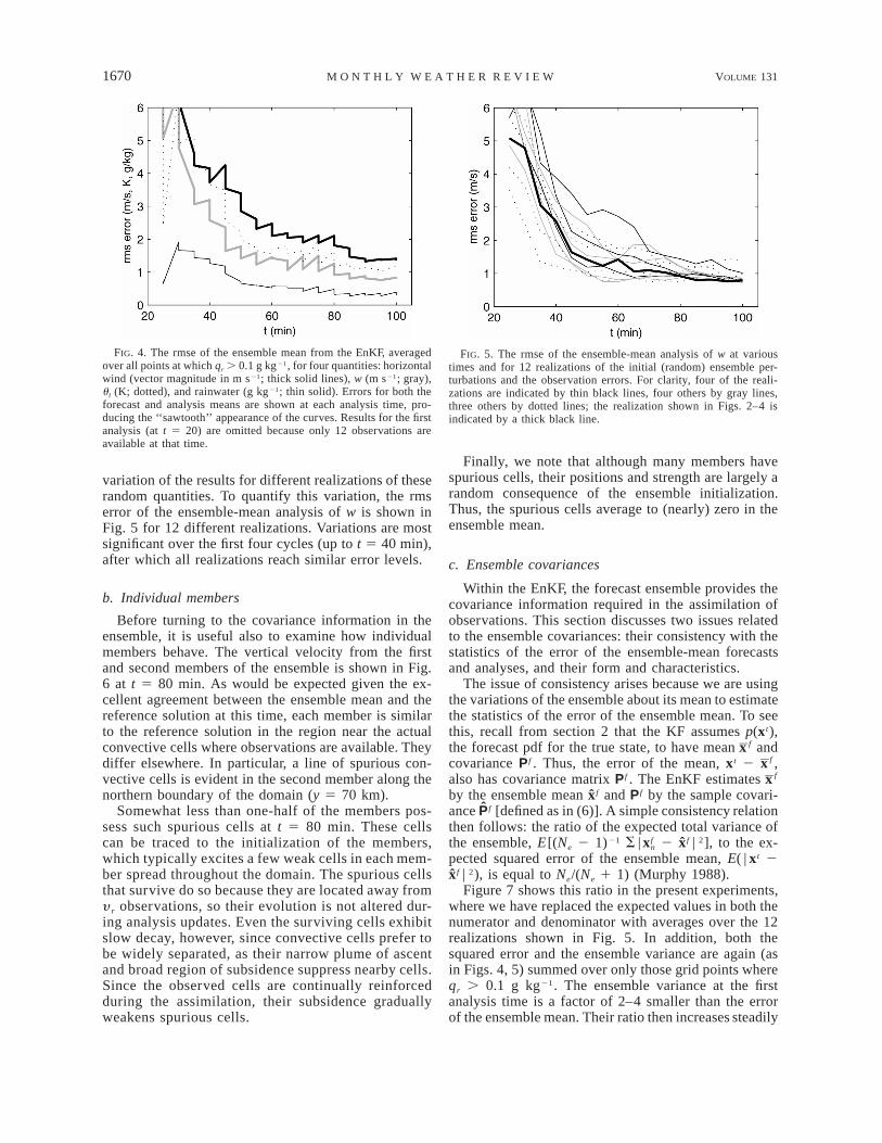
The overall quality of the ensemble-mean forecastsand analyses can be obtained from Fig. 4, where therms errors for the horizontal wind, ul, w, and rainwaterare shown as a function of time. Errors are averagedonly over the portion of the domain where qr . 0.1 gkg21 in order to provide a more accurate and sensitivemeasure of the analysis quality near the cells. (Over therest of the domain, errors tend to be small simply be-cause the variability of the reference simulation aboutthe initial sounding is small.) As was evident in Fig. 3,the analyses improve rapidly over the first 20–30 minof assimilation. The errors in all fields then level off ata magnitude that is small compared to the O(10 m s21,10 K) variations typically found near the convectivecells in the reference solution.

The results shown to this point are all based on asingle set of initial ensemble members. Since the initialensemble is drawn randomly with a specified pdf, as arethe observation errors, one may expect some random


FIG. 4. The rmse of the ensemble mean from the EnKF, averagedover all points at which qr . 0.1 g kg21, for four quantities: horizontalwind (vector magnitude in m s21; thick solid lines), w (m s21; gray),ul (K; dotted), and rainwater (g kg21; thin solid). Errors for both theforecast and analysis means are shown at each analysis time, pro-ducing the ‘‘sawtooth’’ appearance of the curves. Results for the firstanalysis (at t 5 20) are omitted because only 12 observations areavailable at that time.

FIG. 5. The rmse of the ensemble-mean analysis of w at varioustimes and for 12 realizations of the initial (random) ensemble per-turbations and the observation errors. For clarity, four of the reali-zations are indicated by thin black lines, four others by gray lines,three others by dotted lines; the realization shown in Figs. 2–4 isindicated by a thick black line.

variation of the results for different realizations of theserandom quantities. To quantify this variation, the rmserror of the ensemble-mean analysis of w is shown inFig. 5 for 12 different realizations. Variations are mostsignificant over the first four cycles (up to t 5 40 min),after which all realizations reach similar error levels.

b. Individual members

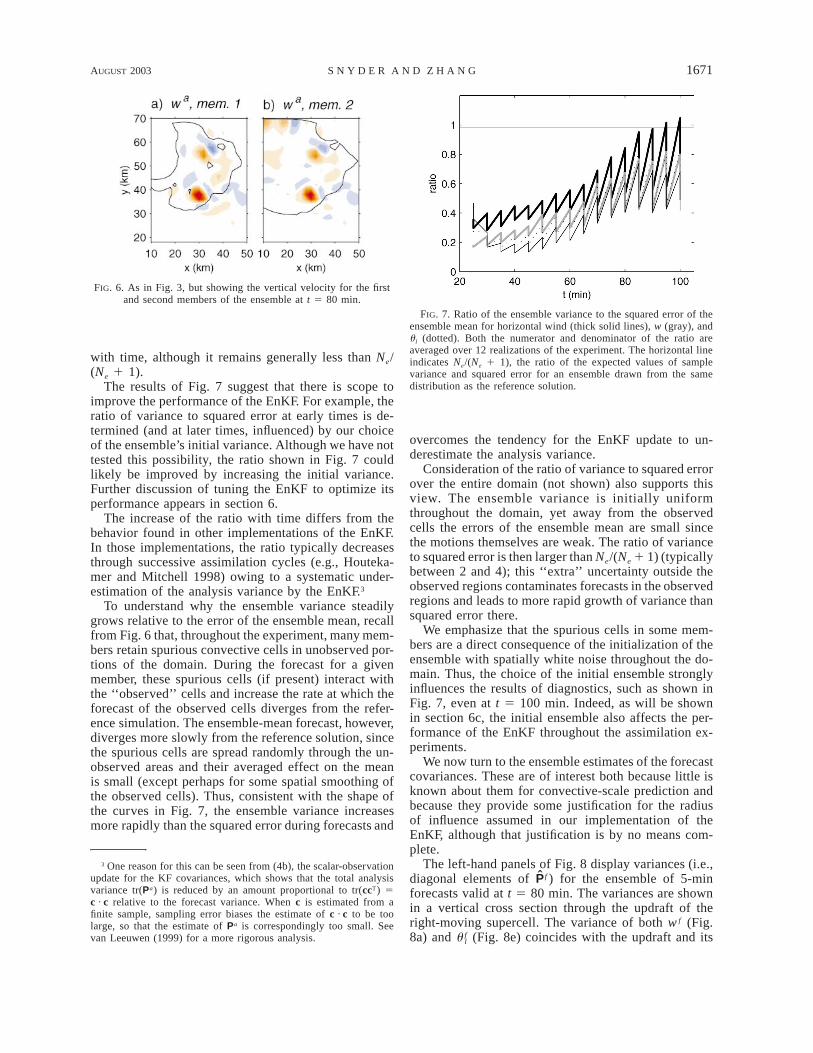
Before turning to the covariance information in theensemble, it is useful also to examine how individualmembers behave. The vertical velocity from the firstand second members of the ensemble is shown in Fig.6 at t 5 80 min. As would be expected given the ex-cellent agreement between the ensemble mean and thereference solution at this time, each member is similarto the reference solution in the region near the actualconvective cells where observations are available. Theydiffer elsewhere. In particular, a line of spurious con-vective cells is evident in the second member along thenorthern boundary of the domain (y 5 70 km).

Somewhat less than one-half of the members pos-sess such spurious cells at t 5 80 min. These cellscan be traced to the initialization of the members,which typically excites a few weak cells in each mem-ber spread throughout the domain. The spurious cellsthat survive do so because they are located away fromy r observations, so their evolution is not altered dur-ing analysis updates. Even the surviving cells exhibitslow decay, however, since convective cells prefer tobe widely separated, as their narrow plume of ascentand broad region of subsidence suppress nearby cells.Since the observed cells are continually reinforcedduring the assimilation, their subsidence graduallyweakens spurious cells.

Finally, we note that although many members havespurious cells, their positions and strength are largely arandom consequence of the ensemble initialization.Thus, the spurious cells average to (nearly) zero in theensemble mean.

c. Ensemble covariances

Within the EnKF, the forecast ensemble provides thecovariance information required in the assimilation ofobservations. This section discusses two issues relatedto the ensemble covariances: their consistency with thestatistics of the error of the ensemble-mean forecastsand analyses, and their form and characteristics.

The issue of consistency arises because we are usingthe variations of the ensemble about its mean to estimatethe statistics of the error of the ensemble mean. To seethis, recall from section 2 that the KF assumes p(xt),the forecast pdf for the true state, to have mean f andxcovariance P f . Thus, the error of the mean, xt 2 f ,xalso has covariance matrix P f . The EnKF estimates fxby the ensemble mean xf and P f by the sample covari-ance P f [defined as in (6)]. A simple consistency relationthen follows: the ratio of the expected total variance ofthe ensemble, E[(Ne 2 1)21 S | 2 xf | 2], to the ex-fxn

pected squared error of the ensemble mean, E( | xt 2xf | 2), is equal to Ne/(Ne 1 1) (Murphy 1988).

Figure 7 shows this ratio in the present experiments,where we have replaced the expected values in both thenumerator and denominator with averages over the 12realizations shown in Fig. 5. In addition, both thesquared error and the ensemble variance are again (asin Figs. 4, 5) summed over only those grid points whereqr . 0.1 g kg21. The ensemble variance at the firstanalysis time is a factor of 2–4 smaller than the errorof the ensemble mean. Their ratio then increases steadily


FIG. 6. As in Fig. 3, but showing the vertical velocity for the firstand second members of the ensemble at t 5 80 min.

FIG. 7. Ratio of the ensemble variance to the squared error of theensemble mean for horizontal wind (thick solid lines), w (gray), andul (dotted). Both the numerator and denominator of the ratio areaveraged over 12 realizations of the experiment. The horizontal lineindicates Ne/(Ne 1 1), the ratio of the expected values of samplevariance and squared error for an ensemble drawn from the samedistribution as the reference solution.

with time, although it remains generally less than Ne/(Ne 1 1).

The results of Fig. 7 suggest that there is scope toimprove the performance of the EnKF. For example, theratio of variance to squared error at early times is de-termined (and at later times, influenced) by our choiceof the ensemble’s initial variance. Although we have nottested this possibility, the ratio shown in Fig. 7 couldlikely be improved by increasing the initial variance.Further discussion of tuning the EnKF to optimize itsperformance appears in section 6.

The increase of the ratio with time differs from thebehavior found in other implementations of the EnKF.In those implementations, the ratio typically decreasesthrough successive assimilation cycles (e.g., Houteka-mer and Mitchell 1998) owing to a systematic under-estimation of the analysis variance by the EnKF.3

To understand why the ensemble variance steadilygrows relative to the error of the ensemble mean, recallfrom Fig. 6 that, throughout the experiment, many mem-bers retain spurious convective cells in unobserved por-tions of the domain. During the forecast for a givenmember, these spurious cells (if present) interact withthe ‘‘observed’’ cells and increase the rate at which theforecast of the observed cells diverges from the refer-ence simulation. The ensemble-mean forecast, however,diverges more slowly from the reference solution, sincethe spurious cells are spread randomly through the un-observed areas and their averaged effect on the meanis small (except perhaps for some spatial smoothing ofthe observed cells). Thus, consistent with the shape ofthe curves in Fig. 7, the ensemble variance increasesmore rapidly than the squared error during forecasts and

3 One reason for this can be seen from (4b), the scalar-observationupdate for the KF covariances, which shows that the total analysisvariance tr(Pa) is reduced by an amount proportional to tr(ccT) 5c · c relative to the forecast variance. When c is estimated from afinite sample, sampling error biases the estimate of c · c to be toolarge, so that the estimate of Pa is correspondingly too small. Seevan Leeuwen (1999) for a more rigorous analysis.

overcomes the tendency for the EnKF update to un-derestimate the analysis variance.

Consideration of the ratio of variance to squared errorover the entire domain (not shown) also supports thisview. The ensemble variance is initially uniformthroughout the domain, yet away from the observedcells the errors of the ensemble mean are small sincethe motions themselves are weak. The ratio of varianceto squared error is then larger than Ne/(Ne 1 1) (typicallybetween 2 and 4); this ‘‘extra’’ uncertainty outside theobserved regions contaminates forecasts in the observedregions and leads to more rapid growth of variance thansquared error there.

We emphasize that the spurious cells in some mem-bers are a direct consequence of the initialization of theensemble with spatially white noise throughout the do-main. Thus, the choice of the initial ensemble stronglyinfluences the results of diagnostics, such as shown inFig. 7, even at t 5 100 min. Indeed, as will be shownin section 6c, the initial ensemble also affects the per-formance of the EnKF throughout the assimilation ex-periments.

We now turn to the ensemble estimates of the forecastcovariances. These are of interest both because little isknown about them for convective-scale prediction andbecause they provide some justification for the radiusof influence assumed in our implementation of theEnKF, although that justification is by no means com-plete.

The left-hand panels of Fig. 8 display variances (i.e.,diagonal elements of P f ) for the ensemble of 5-minforecasts valid at t 5 80 min. The variances are shownin a vertical cross section through the updraft of theright-moving supercell. The variance of both w f (Fig.8a) and (Fig. 8e) coincides with the updraft and itsfu l


FIG. 8. Variances and correlations estimated from the ensemble at t 5 80 min in the x–z plane along y 5 36 km,which passes through the maximum updraft. (left) Variances of (a) w f , (c) u f , and (e) are indicated by black contoursfu l

(at 0.2, 0.4, and 0.8 of the maximum in the cross section); (right) the correlation (black lines, negative values dashed;contours at 60.3 and 60.6) between the forecast value of y r at the point x 5 30 km, z 5 5 km (indicated by a blackdot) and (b) w f , (d) uf , and (f ) at each point in the cross section. Shades of red and blue indicate positive andfu l

negative values, respectively, of fields from the reference solution: (a), (b) w t, with shading increments every 4 m s21

beginning at 62 m s21; (c), (d) ut, with shading as in Figs. 8a,b; and (e), (f ) , with shading increments every 4 Ktu l

beginning at 62 K.

accompanying ul deficit, while Var(u f ) has two maximanear z 5 10 km, one just upstream of the updraft andthe other extending downstream from the updraft. Noneof the variance fields has pronounced maxima near thesurface.

As might be expected given that the EnKF analysesestimate unobserved variables, the ensemble reveals sig-nificant correlations between y r and the state variables.Three examples appear in the right-hand panels of Fig.8, which show the correlation of w f , u f , or at eachfu l

point in the cross section with the forecast value of y r

at a point at the base of the updraft. Like the variances,the correlations reflect the structure of the reference so-lution: for w f and , significant correlations (negativefu l

for w and positive for ul) extend along the height of theupdraft and its accompanying buoyancy deficit. For u f ,strong positive correlations coincide with the region of

weak flow from the base of the updraft upward anddownstream.

Figure 8 provides justification for our choice of a 4-km radius of influence in the assimilation, at least in itsorder of magnitude: that radius is comparable to thescale of variation of the covariances. Moreover, the larg-est covariances are found within that radius of the ob-servation point. It is clear, however, that the 4-km radiusdoes not include all locations with significant covariancewith y r at the observation point, nor does it exclude alllocations with small covariances that are likely stronglycontaminated by sampling error.

Figure 8 also demonstrates that covariances havecomplex structure that is highly inhomogeneous and an-istropic, and are flow dependent in that their structureis related to position and form of the convective cell inreference state. It would likely be difficult to model the


FIG. 9. (a) The rmse for forecasts of w (black lines), starting fromthe ensemble-mean analysis at t 5 30, 45, 60, 80 min and averagedover the entire domain. Errors for the forecast and analysis means ofw are indicated by the gray lines as in Fig. 4 (b) As in Fig. 9a, butfor forecasts starting from initial conditions whose error has beenrescaled by factors of 2 (thin lines), 0.4 (thick), and 0.2 (dotted). Tobe more precise, initial conditions for each forecast are created bycalculating the error of the ensemble-mean analysis at the appropriatetime, multiplying the error field by a constant scalar factor (2, 0.4,0.1), and adding the rescaled error to the reference solution. The rmsefor the original forecast (scale factor of 1) is shown in gray.

covariance structure and its relation to reference statewith just a few parameters.

5. Forecast-error growth

In many geophysical systems, the accuracy of stateestimates is limited in part by forecast-error growth. Itis not obvious, however, that the present system of twoisolated supercells will behave similarly. In particular,each supercell is long lived and quasi-steady, whichindicates that they are at least structurally stable to smallperturbations. This in turn raises the possibility that thedecrease of analysis error with time shown in Figs. 4and 5 arises mainly because forecast errors grow slowlyor decay. This section examines the forecast-errorgrowth in our experiments.

Perhaps the simplest diagnostic is to compare the er-ror of the ensemble-mean 5-min forecast to that of thepreceeding analysis. As can be seen in Fig. 4, errors dotypically grow over the course of the forecast, althoughthere are instances in the initial few cycles in whichdecay occurs.

Errors also grow during longer forecasts. Figure 9ashows rms errors for w for forecasts beginning from theensemble-mean analysis at various times. (Althoughthey are not shown, forecast errors for other variablesbehave similarly. Also note that in Fig. 9 the errors areaveraged over the entire domain.) The time required forthe error to double is roughly 10–20 min in all cases,consistent with the dynamical timescale of the super-cells. Moreover, it is clear that the assimilation of ob-servations with the EnKF provides a significantly betterstate estimate than would be available given only a fore-cast from an earlier time.

Although it does not prevent error growth, the struc-tural stability of the supercells manifests itself in certaincharacteristics of the forecast errors. Specifically, initialerrors can have two effects on the forecast: they mayalter the position and the instantaneous intensity of thesupercells, or they can extinguish one or both cells. Att 5 100 min, for example, the forecasts shown in Fig.9a each contain a right-moving supercell, displaced bya few grid points from that in the reference solution andtypically weaker, while none of the forecasts, exceptthat from t 5 80 min when splitting has already begun,capture the left-moving cell.

In addition, the structural stability of the supercellsmeans that smaller initial errors should produce smallerforecast errors, even beyond the time at which errorgrowth begins to saturate. To test this possibility, wehave performed additional forecasts whose initial con-ditions (at each of the times shown in Fig. 9a) werecreated by scaling the initial error by a factor of 2, 0.4,or 0.1 and then adding that rescaled perturbation to thereference solution. Figure 9b illustrates the results ofthese experiments in terms of the rms error of w. Asexpected, smaller errors at any initial time give rise tosmaller forecast errors through the entire length of the

forecast. In a chaotic system, error growth would pro-ceed from even very small initial errors until the forecastwas completely decorrelated from the reference solu-tion, and the curves in Fig. 9b would, in contrast, allapproach a limiting value with time, regardless of thesize of the initial error. Presumbably, this would alsooccur in a more complex convective situation with mul-tiple cells and outflows.

6. Other issues

a. Importance of covariance information

We have suggested that the EnKF is particularly ap-pealing for use at convective scales because of its abilityto estimate forecast covariances with a minimum of pri-or assumptions, and thereby infer state variables thatare unobserved. Here, we test this assertion with anexperiment in which the EnKF updates only the three


FIG. 10. As in Fig. 5, but for the experiment in which ul, qr, andqt are not updated in the analysis; i.e., observations of y r influenceonly the velocities.

components of the wind given observations of y r, anddoes not use the information available in cross covari-ances between y r and ul, qr and qt.

The rms error of the ensemble-mean analysis of w isshown as a function of time in Fig. 10 for 10 realizationsof the experiments (i.e., for 10 realizations of the initialensemble and 10 realizations of the observation errors).The error is typically more than three times what itwould be if all variables were updated during the anal-ysis (see Fig. 5), and even in the best realization theerror is still doubled. The error in variables other thanw behaves similarly.

Except in the single, anomalously accurate realizationevident in Fig. 10, the analyses (not shown) fail to cap-ture either the updraft or surface cold pool of the ob-served cell at least through t 5 45 min. Instead, theanalyses (and the individual members) contain a noisymix of updrafts and downdrafts spread over the regionof observations, with a variety of spurious cells outsidethat region in individual members. Beyond an hour, theanalyses begin to exhibit narrow updrafts in the loca-tions of the observed cells and small cold pools beneaththese updrafts. The analyzed updrafts then decay mark-edly during the course of the 5-min forecasts to the nextanalysis time.

We have also performed experiments in which theobserved variable is u and only u is updated by theEnKF, so that cross covariances between components ofvelocity are also ignored in the assimilation. Analysiserrors are even larger and the analyses never capturethe updrafts of the observed cells (not shown). Together,these two sets of experiments show that covariancesestimated by the EnKF contain significant informationabout relations among the state variables, despite thesampling errors associated with an ensemble of 50 mem-bers.

b. Tuning of algorithm

To implement EnKF as described here, one mustchoose the ensemble size Ne and the radius of influencefor the observations. Although we have not systemati-cally tuned the algorithm (by determining optimal radiusfor a given Ne), we have performed a number of ex-periments with values other than Ne 5 50 and r 54 km.

It is clear for these additional experiments that theresults in section 4 depend quantitatively on the choiceof Ne and r. In particular, decreasing Ne to 25 increasesthe rms error of the ensemble-mean analyses and alsomakes the results less robust, in the sense that there willbe realizations of the initial ensemble for which theanalyses are always a poor approximation to the ref-erence simulation, as was the case for the experimentsdescribed in section 6a above that did not update ul orthe moisture variables. (Increasing Ne has smaller, butopposite, effects.) For sufficiently large r (roughly 20km or larger, using Ne 5 50), the ensemble-mean anal-ysis noticeably deterioriates and ‘‘outlying’’ realizationsagain become frequent, although more modest varia-tions of r, from 2 to 6 km, have little effect on theanalysis quality. Such dependence on Ne and r is broadlyconsistent with other examples of the EnKF (e.g., Hou-tekamer and Mitchell 1998; Anderson 2001; Whitakerand Hamill 2002).

The results of our experiments also depend on howthe analysis update is performed within the radius r. Amore sophisticated approach is to decrease the influenceof an observation on the state with increasing distancefrom the observation location by multiplying ci in (4a)by a correlation function with local support, as in Hou-tekamer and Mitchell (2001). In this way, the influenceof an observation on the analysis decreases smoothlyto zero at finite radius, rather than jumping discontin-uously to zero. Using such an approach improves theresults presented here (A. Caya 2002, personal com-munication).

Another aspect of the algorithm that can likely beimproved is our choice of the probability distributionfrom which the initial ensemble is drawn. In the resultsjust presented, the initial ensemble is centered on theenvironmental sounding and each member is initializedwith independent Gaussian noise at each grid point andin each variable. Although the initial variance in thissimple scheme could presumably be tuned, we will showin section 6c below that a careful choice of that initialdistribution is likely more important.

A final aspect of ensemble filters that is often subjectto tuning is the covariance inflation (Anderson 2001;Hamill et al. 2001), in which the ensemble covariancesare multiplied by a scalar factor slightly greater than 1to compensate for the usual bias of the EnKF to un-derestimate the analysis uncertainty. We have performedexperiments with several inflation factors and alwaysfind that inflation degrades the results. There appears to


FIG. 11. As in Fig. 5, but for the local perturbations experimentin which the initial ensemble perturbations are nonzero only in a 20km 3 20 km box centered on the location of the first echoes.

FIG. 12. As in Fig. 7, but for the local perturbations experiment.

be two related reasons for this: first, the tendency forthe ensemble forecasts to overestimate, because of thepresence of spurious cells, the growth of variance in theregion of the observed cells; and second, the fact thatthe inflation enhances the spurious cells by increasingdeviations from the ensemble mean. Since the spuriouscells are an artifact of the ensemble initialization, itseems likely that covariance inflation may yet provebeneficial given a more sophisticated initialization. Weleave a more systematic exploration of tuning the EnKFfor subsequent work. The following section providesfurther discussion of the role of the initial ensemble.

c. Dependence on the statistics of the initial ensemble

Sections 4b,c discuss how the initialization of eachmember with noise throughout the domain leads to spu-rious convective cells in many members, which in turndegrade the forecasts from those members and affectthe properties and performance of the EnKF. A naturalquestion is then the extent to which the result might beimproved with a different initialization of the ensemble.

One easy modification, which should reduce the spu-rious cells, is to restrict the initial noise in each memberto the vicinity of the radar echoes. To be more specific,we have performed experiments in which the membersare initialized at t 5 0 with noise confined to a 20 km3 20 km box centered on the location of the first echoes(i.e., the first nonzero values of qr) at t 5 20 min. Exceptfor this restriction of the initial noise to a portion of thedomain, these experiments are identical to those dis-cussed in section 4. Our use of information from t 520 min to initialize the ensemble at t 5 0 is akin thatof 4DVAR or the Kalman smoother (Cohn 1997), inwhich observations influence the state estimate at earliertimes as well as the present time. Note also that thisinitialization is feasible in practice, as one would simplywait until observations were available and then initializethe ensemble at a somewhat earlier time.

The rms error for w is shown in Fig. 11. Analysesare significantly improved over those based on the orig-inal initialization of the ensemble. Averaging over 12realizations of the experiments, error at t 5 50 min isreduced by a factor of 2, while that at t 5 100 min isreduced by a factor of 3.

In the individual members (not shown), some spu-rious cells are still excited by the initial noise, but theseare of course located much closer to the observed cellon average. The subsidence surrounding the observedcell then suppresses the spurious cells more stronglythan in the previous experiments, so that they are weakerthroughout the simulation and almost all have disap-peared by t 5 70 min. The fact that the forecasts fromindividual members are not degraded by the presenceof spurious cells is at least one factor contributing tothe improved performance of the EnKF.

In section 4c, we also argued that the presence ofspurious cells in some members led to a continual in-crease in the ensemble variance relative to the squarederror of the ensemble mean. Figure 12 shows the ratioof these quantities for the present ‘‘local perturbation’’experiment and should be compared to Fig. 5. The ratioof variance to error increases through the first half ofboth experiments. By t 5 70 min, the ratio stops itssystematic increase in the local perturbation experiment;this coincides with the time at which most spurious cellshave been suppressed.

7. Summary and discussion

In the experiments presented here, we have used theEnKF to assimilate simulated Doppler radar observa-tions of radial velocity in a nonhydrostatic, cloud-scalemodel. The observations are taken (together with ran-dom observational noise) from a reference simulationof a splitting supercell storm, produced with the samenumerical model. We assume that observations areavailable every 5 min, but only in the small fraction ofthe domain where the rainwater in the reference simu-lation exceeds a threshold.


These experiments demonstrate the potential of theEnKF for assimilation of radar data at the convectivescale. Using an ensemble of 50 members, the EnKFproduces analyses that accurately approximate the truestate (i.e., that from the reference simulation) after aboutseven assimilation cycles and a half hour of observa-tions. Variables not directly observed, including the ver-tical velocity and temperature, are accurately estimatedin the analyses. Examination of forecasts also showsthat the simple supercell simulation considered here sup-ports significant growth of forecast error and, thus, thatthe ability of the EnKF to track the growth and splittingof the cell is not simply a consequence of stable systemdynamics.

In principle, the crucial element of the EnKF is itsdirect estimate of forecast covariances between radialvelocity (or other observed quantities) and the state var-iables. To test the importance of such covariances, wealso performed experiments in which the covariancesof y r with the thermodynamic and moisture variableswere set to zero in the assimilation, so that the obser-vations did not influence the analyses of temperature,moisture, and cloud water. The rms analysis error morethan tripled in these experiments.

It is worth emphasizing that the dynamics of moistconvection represents a significant test for the EnKF.Unlike the large-scale flows in the atmosphere or basinscales in the ocean, which have been the setting of allprevious implementations of the EnKF, convective-scalemotions generally lack approximate, static balances,such as geostrophy, that link the velocity to thermo-dynamic fields. Our results indicate that the lack of suchbalances is not a fundamental obstacle to the use of theEnKF at convective scales, as the dynamically producedrelations among state variables (i.e., those that arisethrough the evolution of the flow) are sufficiently strongand develop rapidly. In addition, moist convection isdriven by distinctly nonlinear microphysical processes,such as condensation, and tends to form discrete, co-herent structures, such as supercells, whose dynamicsare nonlinear; both of these facts call into question theGaussian assumptions that underlie the EnKF analysisstep. The success of the EnKF in the present problemsuggests that the nonlinearity inherent in moist convec-tion is also not a fundamental obstacle to the EnKF.Nevertheless, continued development of the EnKF forconvective scales will undoubtedly require further con-sideration of nonlinear and non-Gaussian effects, par-ticularly in relation to reflectivity observations.

Our experiments also differ from those of previousstudies with the EnKF in that they cover a limited timeinterval, spanning only a few dynamical timescales. Thequality of the analyses, and even diagnostics of the per-formance of the scheme such as the ratio of variance toerror, are therefore strongly influenced throughout ourexperiments by the choice of the initial ensemble. Aparticular example appears in section 6c. (In contrast,other studies have collected results over long simula-

tions of systems that possess a statistically steady state,so that the initial ensemble is not important.) Althoughthe initial conditions for the ensemble should clearlyreflect our best knowledge of p(xt) prior to any obser-vations, considerable latitude remains for choosing themreasonably. We expect that improving the initial ensem-ble and diagnosing its role are likely to be persistentissues for the EnKF at convective scales.

The performance of the EnKF relative to retrievaltechniques or 4DVAR is an important question that wehave not addressed in this paper. In fact, our use the ofthe model of Sun and Crook (1997) was motivated bythe possibility of comparing against the existing 4DVARscheme for that model. Comparisons are under way andwill be reported elsewhere (A. Caya and J. Sun 2003,personal communication).

There are a number of other important issues that werebeyond the scope of this initial paper. These include theuse of reflectivity observations; estimation of the en-vironmental sounding and its uncertainty; accountingfor imperfections in the forecast model, particularly themicrophysical parameterizations; the treatment of lateralboundary conditions and their uncertainty; and quan-tification of errors in real radar observations and in theforward operators for both radial velocity and reflectiv-ity, as well as quality control for radar observations.Progress on all of these issues is likely important if theEnKF, or indeed another technique, is to be applied rou-tinely and successfully to the assimilation of radar ob-servations.

Acknowledgments. We are particularly indebted toJuanzhen Sun for the use of her cloud model in thisstudy. Both Alain Caya and David Dowell have sharedwith us their results related to various refinements ofthe algorithm used here. It is a pleasure to acknowledgehelpful discussions with them and with William Ska-marock and Jeff Anderson. This research was supportedat NCAR by the U.S. Weather Research Program andby NSF Grant 0205655.

REFERENCES

Anderson, J. L., 2001: An ensemble adjustment filter for data assim-ilation. Mon. Wea. Rev., 129, 2884–2903.

Brusdal, K., J. M. Brankart, G. Halberstadt, G. Evensen, P. Brasseur,P. J. van Leeuwen, E. Dombrowsky, and J. Verron, 2003: Ademonstration of ensemble based assimilation methods with alayered OGCM from the perspective of operational ocean fore-casting systems. J. Mar. Syst., 40–41, 253–289.

Cohn, S. E., 1997: An introduction to estimation theory. J. Meteor.Soc. Japan, 75, 257–288.

Evensen, G., 1994: Sequential data assimilation with a nonlinear qua-si-geostrophic model using Monte Carlo methods to forecasterror statistics. J. Geophys. Res., 99 (C5), 10 143–10 162.

Hamill, T. M., and C. Snyder, 2000: A hybrid ensemble Kalman filter/3D-variational analysis scheme. Mon. Wea. Rev., 128, 2905–2919.

——, J. S. Whitaker, and C. Snyder, 2001: Distance-dependent fil-tering of background error covariance estimates in an ensembleKalman filter. Mon. Wea. Rev., 129, 2776–2790.


Houtekamer, P. L., and H. L. Mitchell, 1998: Data assimilation usingan ensemble Kalman filter technique. Mon. Wea. Rev., 126, 796–811.

——, and ——, 2001: A sequential ensemble Kalman filter for at-mospheric data assimilation. Mon. Wea. Rev., 129, 123–137.

Ide, K., P. Courtier, M. Ghil, and A. C. Lorenc, 1997: Unified notationfor data assimilation: Operational, sequential, and variational. J.Meteor. Soc. Japan, 75, 181–189.

Keppenne, C. L., and M. M. Rienecker, 2002: Initial testing of amassively parallel ensemble Kalman filter with the Poseidonisopycnal ocean general circulation model. Mon. Wea. Rev., 130,2951–2965.

Leith, C. E., 1983: Predictability in theory and practice. Large-ScaleDynamical Processes in the Atmosphere, B. J. Hoskins and R.P. Pearce, Eds., Academic Press, 365–383.

Mitchell, H. L., and P. L. Houtekamer, 2000: An adaptive ensembleKalman filter. Mon. Wea. Rev., 128, 416–433.

——, ——, and G. Pelerin, 2002: Ensemble size, balance, and model-error representation in an ensemble Kalman filter. Mon. Wea.Rev., 130, 2791–2808.

Montmerle, T., A. Caya, and I. Zawadzki, 2001: Simulation of amidlatitude convective storm initialized with bistatic Dopplerradar data. Mon. Wea. Rev., 129, 1949–1967.

Murphy, J. M., 1988: The impact of ensemble forecasts on predict-ability. Quart. J. Roy. Meteor. Soc., 114, 463–493.

Rabier, F., H. Jarvinen, E. Klinker, J.-F. Mahfouf, and A. Simmons,2000: The ECMWF operational implementation of four-dimen-sional variational assimilation. Part I: Experimental results withsimplified physics. Quart. J. Roy. Meteor. Soc., 126, 1143–1170.

Sun, J., and N. A. Crook, 1997: Dynamical and microphysical re-trieval from Doppler radar observations using a cloud model andits adjoint. Part I: Model development and simulated data ex-periments. J. Atmos. Sci., 54, 1642–1661.

——, and ——, 1998: Dynamical and microphysical retrieval fromDoppler radar observations using a cloud model and its adjoint.Part II: Retrieval experiments of an observed Florida convectivestorm. J. Atmos. Sci., 55, 835–852.

van Leeuwen, P. J., 1999: Comments on ‘‘Data assimilation using anensemble Kalman filter technique.’’ Mon. Wea. Rev., 127, 1374–1377.

Weygandt, S. S., A. Shapiro, and K. K. Droegemeier, 2002: Retrievalof model initial fields from single-Doppler observations of asupercell thunderstorm. Part I: Single-Doppler velocity retrieval.Mon. Wea. Rev., 130, 433–453.

Whitaker, J. S., and T. M. Hamill, 2002: Ensemble data assimilationwithout perturbed observations. Mon. Wea. Rev., 130, 1913–1924.

Xu, Q., H. D. Gu, and S. Yang, 2001: Simple adjoint method forthree-dimensional wind retrievals from single-Doppler data.Quart. J. Roy. Meteor. Soc., 127, 1053–1067.

assimilation of simulated doppler radar observations with...

Documents