Data Assimilation

Alan O’Neill

National Centre for Earth Observation

&

University of Reading

Contents

• Motivation

• Univariate (scalar) data assimilation

• Multivariate (vector) data assimilation– Optimal Interpoletion (BLUE)

– 3d-Variational Method

– Kalman Filter

– 4d-Variational Method

• Applications of data assimilation in earthsystem science

Motivation

What is data assimilation?

Data assimilation is the technique

whereby observational data are

combined with output from a

numerical model to produce an

optimal estimate of the evolving

state of the system.

DARC

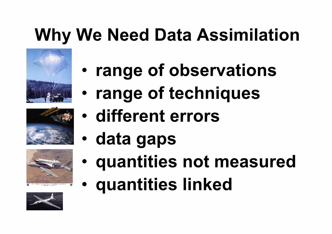
Why We Need Data Assimilation

• range of observations

• range of techniques

• different errors

• data gaps

• quantities not measured

• quantities linked

Preliminary Concepts

What We Want To Know

c

s

x

)(

)(

t

t atmos. state vector

surface fluxes

model parameters

)),(),(()( csxX ttt =

What We Also Want To Know

Errors in models

Errors in observations

What observations to make

Numerical

ModelDAS

DATA ASSIMILATION SYSTEM

O

Data

Cache

A

A

B

F

model

observations

Error Statistics

The Data Assimilation Process

observations forecasts

estimates of state & parameters

compare

reject

adjust

errors in obs. & forecasts

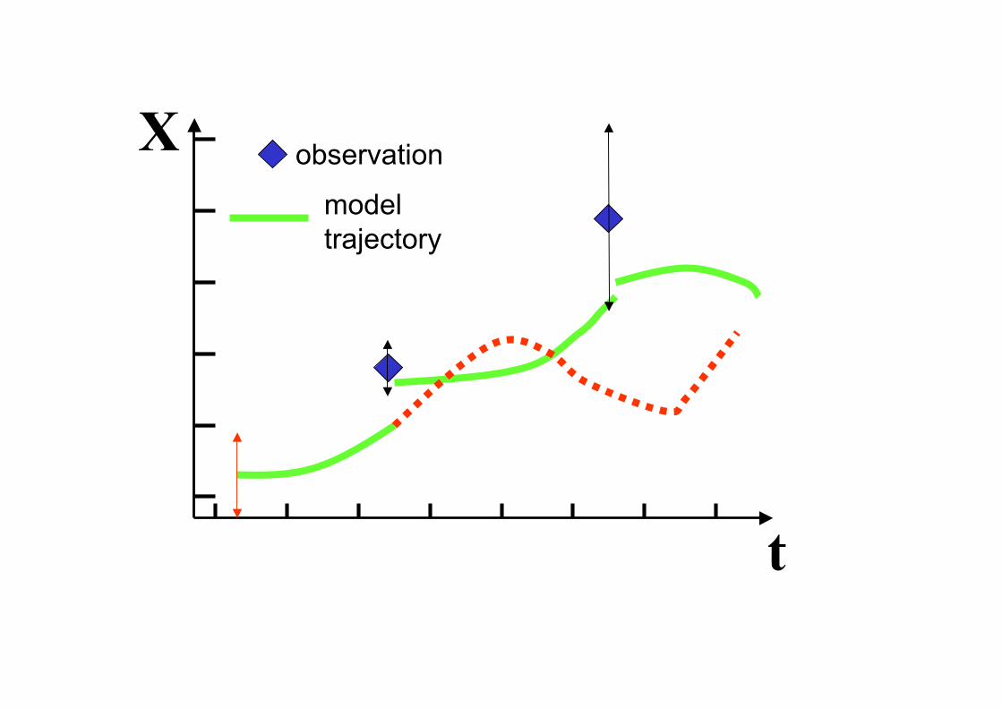
X

t

observation

model

trajectory

Basic Concept of

Data Assimilation

• Information is accumulated in time into

the model state and propagated to all

variables.

What are the benefits of

data assimilation?

• Quality control

• Combination of data

• Errors in data and in model

• Filling in data poor regions

• Designing observational systems

• Maintaining consistency

• Estimating unobserved quantities

DARC

Some Uses of

Data Assimilation (state

estimation, inverse modelling)• Satellite retrievals

• Operational weather and ocean forecasting

• Seasonal weather forecasting

• Land-surface process

• Surface-flux estimation

• Model parameter estimation

• Global climate datasets

• Planning satellite measurements

• Evaluation of models and observations

DARC

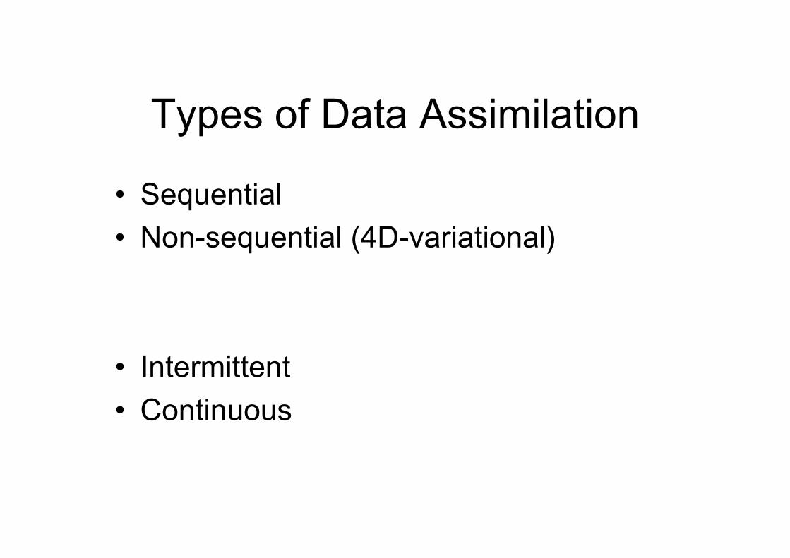
Types of Data Assimilation

• Sequential

• Non-sequential (4D-variational)

• Intermittent

• Continuous

Sequential Intermittent

Assimilation

analysis analysisanalysismodel model

obsobsobsobsobs obs

Non-sequential Continuous

Assimilation

analysis + model

obsobs

obsobsobs

obs

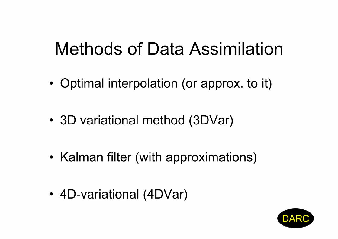
Methods of Data Assimilation

• Optimal interpolation (or approx. to it)

• 3D variational method (3DVar)

• Kalman filter (with approximations)

• 4D-variational (4DVar)

DARC

Statistical Approach to

Data Assimilation

DARC

Data Assimilation

Made Simple

(scalar case)

Least Squares Method

(Minimum Variance)

1

:unbiased be should analysis The

nsobservatio theofn combinatiolinear a as Estimate

eduncorrelat are tsmeasuremen twothe,0

)(

)(

0

21

2211

t

21

2

2

2

2

2

1

2

1

21

22

11

=+!

>>=<<

+=

>=<

>=<

>=<

>=>=<<

+=

+=

aa

TT

TaTaT

T

TT

TT

ta

a

t

t

""

#"

#"

""

"

"

Least Squares Method

Continued

0 constraint thesubject to

)(

))()(()(

:error squaredmean its minimizingby Estimate

21

2

22

2

1

2

21

2

2211

22

=+

+>=+=<

>!+!>=<!=<

111

aa

aaaa

TTaTTaTT

T

tttaa

a

""##

"

Least Squares Method

Continued

2

2

2

2

111

1

!!

!

+=

1

1a

2

2

2

2

2

211

1

!!

!

+=

1

a

2

2

2

1

2

111

!!!+="

a

The precision of the analysis is the sum of the precisions

of the measurements. The analysis therefore has higher

precision than any single measurement (if the statistics

are correct).

Maximum Likelihood Estimate

• Obtain or assume probability distributions for

the errors

• The best estimate of the state is chosen to

have the greatest probability, or maximum

likelihood

• If errors normally distributed,unbiased and

uncorrelated, then states estimated by

minimum variance and maximum likelihood

are the same

Maximum Likelihood Approach

(Bayesian Derivation)

pdf.prior the2

)(exp )(

:is statisticserror Gaussian for

truth theofon distributiy probabilit Then the

on).assimilati datain forecast background the(

,n observatioan madealready have weAssume

2

2

1

1

!!"

#$$%

& ''(

1)

TTTp

T

T

Maximum Likelihood

Continued

).statisticsGaussian (for case ldimensiona-multifor holds eEquivalenc

function.cost theminimizing asanswer same get the We

truth. theestimate toln)(or pdfposterior theMaximize

T. oft independenfactor gnormalisin is )( since

2

)(exp

2

)(exp

)(

)()|()|(

:is n observatio given the pdfposterior for the formula sBayes'

2

2

1

2

1

2

2

2

2

2

22

2

Tp

TTTT

Tp

TpTTpTTp

T

!!"

#$$%

& ''!

!"

#$$%

& ''(=

))

Variational Approach

0for which of value theis

)()(

2

1)(

2

2

2

2

2

2

1

=!

!

"#

$%&

' (+

(=

1

TJTT

TTTTTJ

a

))

)(TJ

T

Simple Sequential Assimilation

1

2 2 2 1

2 2

Let

( ) where ( ) is the "innovation".

The optimal weight is given by:

( ) , and the analysis error variance is:

(1 )

b o

a b o b o b

b b o

a b

T T T T

T T W T T T T

W

W

W

! ! !

! !

"

= =

= + " "

= +

= "

Comments

• The analysis is obtained by adding first

guess to the innovation.

• Optimal weight is background error variance

multiplied by inverse of total variance.

• Precision of analysis is sum of precisions of

background and observation.

• Error variance of analysis is error variance of

background reduced by (1- optimal weight).

Simple Assimilation Cycle

• Observation used once and then

discarded.

• Forecast phase to update and

• Analysis phase to update and

• Obtain background as

• Obtain variance of background as

bT

2

b!

aT

2

a!

)]([)( 1 iaibtTMtT =+

)()(ely alternativ )()(2

1

22

1

2

iaibibibtattt !!!! == ++

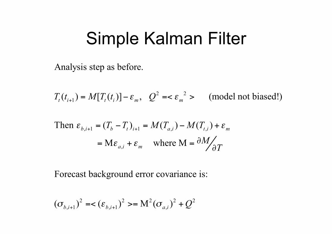
Simple Kalman Filter

2 2

1

, 1 1 , ,

,

Analysis step as before.

( ) [ ( )] , (model not biased!)

Then ( ) ( ) ( )

M where M

Forecast background error covariance

t i t i m m

b i b t i a i t i m

a i m

T t M T t Q

T T M T M T

MT

! !

! !

! !

+

+ +

= " =< >

= " = " +

#= + =#

2 2 2 2 2

, 1 , 1 ,

is:

( ) ( ) M ( )b i b i a i Q$ ! $+ +

=< >= +

Multivariate Data Assimilation

Multivariate Case

!!!!!

"

#

$$$$$

%

&

=

nx

x

x

t2

1

)(x vector state

!!!

"

#

$$$

%

&

=

my

y

y

t 2

1

)( vector nobservatio y

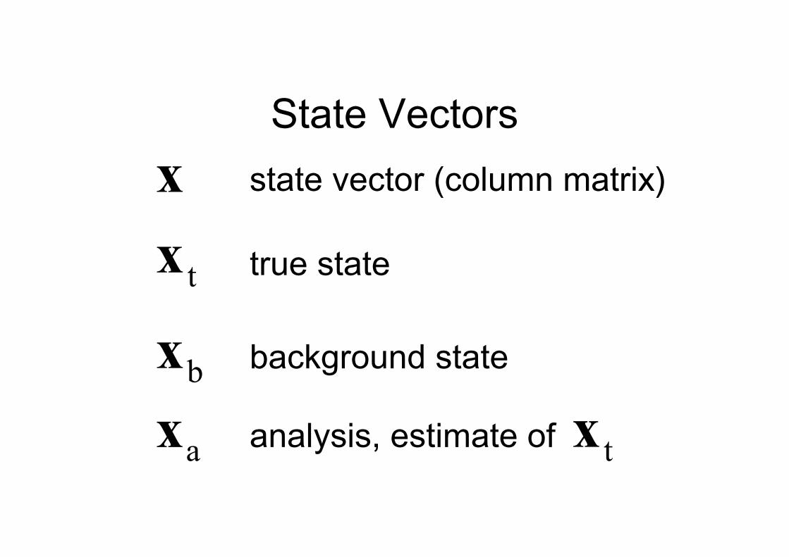
State Vectors

x

bx

tx

ax

state vector (column matrix)

true state

background state

analysis, estimate oftx

Ingredients of Good Estimate

of the State Vector (“analysis”

• Start from a good “first guess” (forecastfrom previous good analysis)

• Allow for errors in observations andfirst guess (give most weight to datayou trust)

• Analysis should be smooth

• Analysis should respect knownphysical laws

Some Useful Matrix Properties

inversion) through conserved isproperty this(

. unless 0,scalar the,

:matrix symmetrix for ssdefinitene Positive

)()( : transposea of Inverse

)( :product a of Inverse

)( :product a of Transpose

T

T11T

111

TTT

0xxAxx

A

AA

ABAB

ABAB

=>!

=

=

=

""

"""

Observations

• Observations are gathered into an

observation vector , called the

observation vector.

• Usually fewer observations than variables in

the model; they are irregularly spaced; and

may be of a different kind to those in the

model.

• Introduce an observation operator to map

from model state space to observation space.

y

)(xx H!

Errors

Variance becomes

Covariance Matrix

• Errors in xi are often correlated

– spatial structure in flow

– dynamical or chemical relationships

• Variance for scalar case becomes

Covariance Matrix for vector case COV

• Diagonal elements are the variances of xi

• Off-diagonal elements are covariances

between xi and xj

• Observation of xi affects estimate of xj

The Error Covariance Matrix

( )

!!!!!!!!

"

#

$$$$$$$$

%

&

><><><

><><><

><><><

>==<

=

!!!!!!!!

"

#

$$$$$$$$

%

&

=

nnnn

n

n

n

n

eeeeee

eeeeee

eeeeee

eee

e

e

e

...

......

......

......

...

...

...

.

.

.

21

22212

12111

T

21

T

2

1

''

''

P

2

iiiee !>=<

Background Errors

• They are the estimation errors of the

background state:

• average (bias)

• covariance

tbbxx !="

><b!

>><!><!=<T

bb ))(( """"B

Observation Errors

• They contain errors in the observation

process (instrumental error), errors in

the design of , and

“representativeness errors”, i.e.

discretization errors that prevent

from being a perfect representation of

the true state.

H

tx

)( to xy H!=" ><o!

>><!><!=<T

oooo ))(( """"R

Control Variables

• We may not be able to solve the

analysis problem for all components of

the model state (e.g. cloud-related

variables, or need to reduce resolution)

• The work space is then not the model

space but the sub-space in which we

correct , called control-variable

spacebx

xxx !+=ba

Innovations and Residuals

• Key to data assimilation is the use ofdifferences between observations andthe state vector of the system

• We call the innovation

• We call the analysis

residual

)( bxy H!

)( axy H!

Give important information

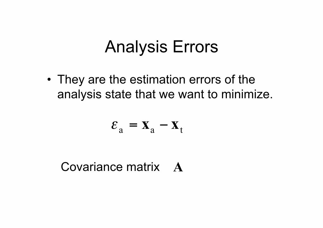
Analysis Errors

• They are the estimation errors of the

analysis state that we want to minimize.

taaxx !="

Covariance matrix A

Using the Error

Covariance Matrix

Recall that an error covariance matrix

for the error in has the form:

T>=< !!C

If where is a matrix, then

the error covariance for is given by:

Hxy = H

x

yT

HCHC =y

C

BLUE Estimator

• The BLUE estimator is given by:

• The analysis error covariance matrix is:

• Note that:

1TT

bba

)(

))((

!+=

!+=

RHBHBHK

xyKxx H

BKHIA )( !=

1T11T11TT )()( !!!!!+=+ RHHRHBRHBHBH

Statistical Interpolation with

Least Squares Estimation

• Called Best Linear Unbiased Estimator

(BLUE).

• Simplified versions of this algorithm

yield the most common algorithms

used today in meteorology and

oceanography.

Assumptions Used in BLUE• Linearized observation operator:

• and are positive definite.

• Errors are unbiased:

• Errors are uncorrelated:

• Linear analysis: corrections to backgrounddepend linearly on (background – obs.).

• Optimal analysis: minimum variance estimate.

)()()( bb xxHxx !=!HH

B R

0)( ttb >=!>=<!< xyxx H

0))()(( T

ttb >=!!< xyxx H

Optimal Interpolation

))(( bba xyKxx H!+=

“analysis”

“background”

(forecast)

observation

1RHBHBHK

-+= )(TT

• linearity H H

• matrix inverse

• limited area

observation

operator

!

!

!

!

!

!!

!

)( bxy H!=" at obs. point

bx

data void

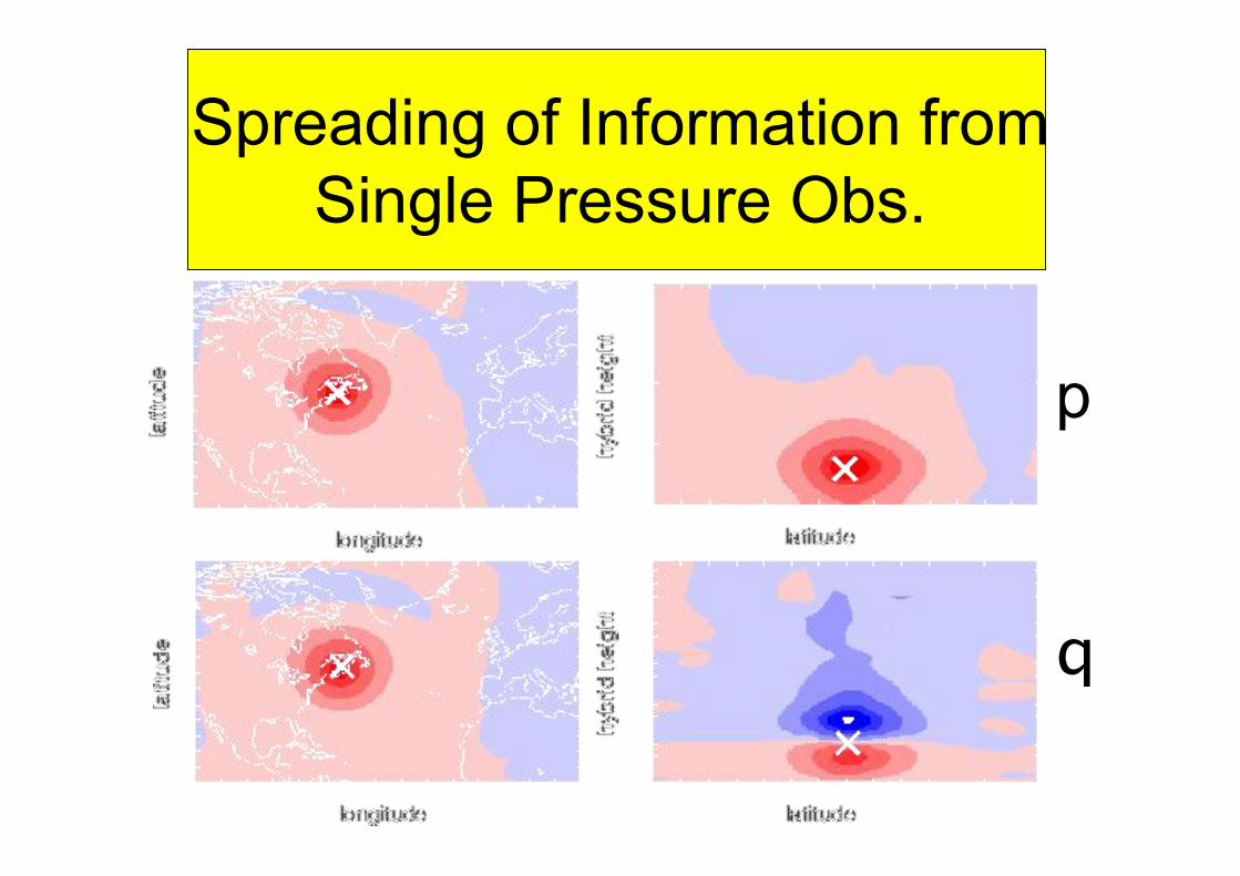
Spreading of Information from

Single Pressure Obs.

p

q

MIPAS observations 6 day model forecast

Analysis

Ozone at 10hPa, 12Z 23rd Sept 2002

bx

3D variational data assimilation - ozone at 10hPa

bx )(

bh xy !

3D variational data assimilation - ozone at 10hPa

bx )(

bh xy !

))((b

h xyK !

3D variational data assimilation - ozone at 10hPa

bx )(

bh xy !

))((bb

h xyKx !+ ))((b

h xyK !

The data assimilation cycle: ozone at 10hPa

Estimating Error Statistics

• Error variances reflect our uncertainty in the

observations or background.

• Often assume they are stationary in time and

uniform over a region of space.

• Can estimate by observational method or as

forecast differences (NMC method).

• More advanced, flow dependent errors

estimated by Kalman filter.

Estimating Covariance Matrix

for Observations, O

• O usually quite simple:

– diagonal or

– for nadir-sounding satellites, non-zero

values between points in vertical only

• Calibration against independent

measurements

Estimating the Error Covariance

Matrix B

• Model B with simple functions basedon comparisons of forecasts withobservations:

• Error growth in short-range forecasts“verifying” at the same time (NMCmethod)

>!!"<T)]24()48()][24()48([ hhhh ffff xxxxB

state vector at time t from forecast 48h or 24 h earlier

)exp( LdB ijjiij !" ## horiz. fn x vert. fn

3d-Variational Data

Assimilation

Variational Data Assimilation

)(xJ

x

vary

to minimise

x

)(xJ

ax

Equivalent Variational

Optimization Problem• BLUE analysis can be obtained by

minimizing a cost (penalty, performance)function:

• The analysis is optimal (closest in least-squares sense to ).

• If the background and observation errors areGaussian, then is also the maximumlikelihood estimator.

J

JJJ

HHJ

min

)()()(

))(())(()()()(

a

ob

1T

b

1T

b

=

+=

!!+!!=!!

x

xxx

xyRxyxxBxxx

ax

tx

ax

Remarks on 3d-VAR

• Can add constraints to the costfunction, e.g. to help maintain “balance”

• Can work with non-linear observationoperator H.

• Can assimilate radiances directly(simpler observational errors).

• Can perform global analysis instead ofOI approach of radius of influence.

))(())((

)()(

)(

1

1

xyRxy

xxBxx

x

HH

J

T

b

T

b

!!

+!!

=

!

!

Variational Data Assimilation

nonlinear operator

assimilate y

directly global

analysis

Maximum Probability or

Likelihood• For Gaussian errors the background,

observation and analysis pdfs are:

where b, o, and a are normalizing factors.

• Maximum probability estimate minimizes

T 1

b b b

T 1

o

a b o

( ) b exp[( ) ( )]

( ) o exp[( ( )) ( ( ))]

( ) a ( ) ( )

P

P H H

P P P

!

!

= ! !

= ! !

=

x x x B x x

x y x R y x

x x x

)(ln)( a xx PJ !=

Comments

• Biases occur in background and observations.

Remove them if known, otherwise analysis is

sub-optimal. Monitor (O-B), but is the bias in

the model or in observations?

• B and O errors usually uncorrelated, but could

be correlations in satellite retrievals.

• Error in the linearization of H should be much

smaller than observational errors for all values

of met in the analysis procedure.bxx !

Choice of State Variables and

Preconditioning

• Free to choose which variables to use to

define state vector, x(t)

• We’d like to make B diagonal

– may not know covariances very well

– want to make the minimization of J more

efficient by “preconditioning”: transforming

variables to make surfaces of constant J

nearly spherical in state space

x2

x1

Cost Function for Correlated Errors

x2

x1

Cost Function for

Uncorrelated Errors

x2

x1

Cost Function for

Uncorrelated Errors

Scaled Variables

The Kalman Filter

Kalman Filter

(expensive)

Use model equations to

propagate B forward in time.

B B(t)

Analysis step as in OI

Evolution of Covariance Matrices

adjoint. its is ;model"linear tangent " theis

where)()()(

))((

)( :is covarianceerror forecast The

:Subtract

)(

modellinear -non theis where)(

T

TT

T11

1

1

1

1

MM

QQMPM

PB

M

xx

xx

>=<+=

>=<

=

+=

!=

=

++

+

+

+

+

mmnnan

n

b

n

b

nf

m

n

a

n

b

m

n

t

n

t

n

a

n

b

ttt

t

M

MM

""

""

"""

"

HRHBP1T11 !!!

+=a

t

The Kalman Filter

1x

2x

Remarks

• In OI (and 3d-VAR) isolated observation

given more weight than observations close

together (forecast errors have large

correlations at nearby observation points).

• When several observations are close

together calculation of weights may be ill-

posed. Therefore combine into a “super

observation”.

Extended Kalman Filter

• Assumes the model is non-linear and

imperfect.

• The tangent linear model depends on the

state and on time.

• Could be a “gold standard” for data

assimilation, but very expensive to

implement because of the very large

dimension of the state space (~ 106 – 107 for

NWP models).

Ensemble Kalman Filter

• Carry forecast error covariance matrixforward in time by using ensembles offorecasts:

• Only ~ 10 + forecasts needed.

• Does not require computation of tangentlinear model and its adjoint.

• Does not require linearization of evolution offorecast errors.

• Fits in neatly into ensemble forecasting.

T

1

))((1

1><!><!

!" #

$

ff

k

fK

k

f

k

f

KxxxxP

4d-Variational Assimilation

4D Variational Data Assimilation

given X(to), the

forecast is

deterministic

vary X(to) for best fit to datato t

obs.

&

errors

4d-VAR For Single Observation

at time t

1x

2x

t

0x

x

yxx =)~( e wher~H

)),(( 0 tJ xx

4d-Variational Assimilation

constraint strong a as

treatedis model thei.e. ))(()( where

)]()([)]()([2

1

)]([)]([2

1))((

00

00

1

0

T

00

1T

0

0

tMt

tttt

HHtJ

ii

bb

iiii

N

i

i

xx

xxBxx

xyRxyx

!

"

"

=

=

""+

""= #

Minimize the cost function by finding the gradient

(“Jacobian”) with respect to the control variables in

)( 0tJ x!

)( 0tx

4d-VAR Continued

The 2nd term on the RHS of the cost function

measures the distance to the background

at the beginning of the interval. The term

helps join up the sequence of optimal

trajectories found by minimizing the cost

function for the observations. The “analysis”

is then the optimal trajectory in state space.

Forecasts can be run from any point on the

trajectory, e.g. from the middle.

xx a0

:M

Some Matrix Algebra

Azx

z

x

x

x

Azx

z

x

xAzxz

xx

x

x

xx

TT

00

T

T

T

00

0

:results theseCombining

shown that becan it Then

)()( :form following thehave Let

Then

))((

!"

#$%

&

'

'!!"

#$$%

&

'

'=

'

'

!"

#$%

&

'

'=

'

'

=

'

'!!"

#$$%

&

'

'=

'

'

=

J

J

JJ

JJ

JJ adjoint of the model

4d-VAR for Single Observation

MTL of time

in n integratio backward...

...

modellinear

tangentofadjoint ,)(

where

))](([

:Algebra"Matrix Some" slideon results usingBy

))](([))](([2

1))((

TTT

0

T

0

00

0

0

T

0

T

0

T

0

T

00

1TT

0

0

0

1T

00

1211

1211

!="

=

#

#=$$

%

&''(

)

#

#=

*+**=#

#

**=

,,,,

,,,,

,,

,*

,

*

*

*

tttttt

tttttt

t

t

tt

n

n

M

HJ

HHJ

LLLL

LLLL

x

x

x

xL

dLxxyRHLx

xxyRxxyxxobs. term only

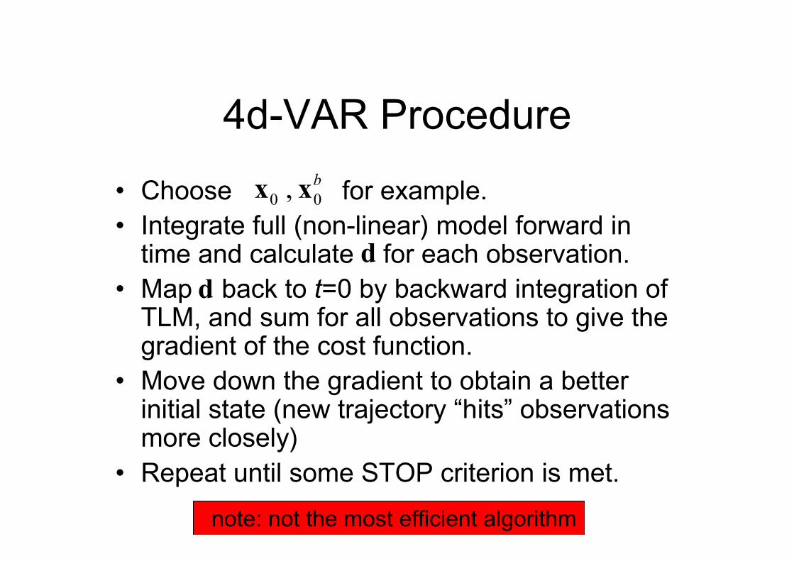
4d-VAR Procedure

• Choose for example.

• Integrate full (non-linear) model forward intime and calculate for each observation.

• Map back to t=0 by backward integration ofTLM, and sum for all observations to give thegradient of the cost function.

• Move down the gradient to obtain a betterinitial state (new trajectory “hits” observationsmore closely)

• Repeat until some STOP criterion is met.

note: not the most efficient algorithm

b

00 , xx

d

d

Comments• 4d-VAR can also be formulated by the method of

Lagrange multipliers to treat the model equations asa constraint. The adjoint equations that arise in thisapproach are the same equations we have derivedby using the chain rule of partial differentialequations.

• If model is perfect and B0 is correct, 4d-VAR at finaltime gives same result as extended Kalman filter(but the covariance of the analysis is not available in4d-VAR).

• 4d-VAR analysis therefore optimal over its timewindow, but less expensive than Kalman filter.

Incremental Form of 4d-VAR

• The 4d-VAR algorithm presented earlier is

expensive to implement. It requires repeated

forward integrations with the non-linear

(forecast) model and backward integrations

with the TLM.

• When the initial background (first-guess)

state and resulting trajectory are accurate, an

incremental method can be made much

cheaper to run on a computer.

Incremental Form of 4d-VAR

]),())(([]),())(([2

1

)()(2

1)(

by defined isfunction cost theof form lincrementa The

00

T

00

0

0

1

0

T

00

xLHxyxLHxy

xBxx

!!

!!!

iii

f

ii

N

i

ii

f

i tttHtttH

J

""""+

=

#=

"

Taylor series expansion

about first-guess trajectory

)( if tx

Minimization can be done in lower dimensional space

)()( where 000 ttbxxx !="

4D Variational Data Assimilation

• Advantages– consistent with the governing eqs.

– implicit links between variables

• Disadvantages– very expensive

– model is strong constraint

Some Useful References

• Atmospheric Data Analysis by R. Daley, CambridgeUniversity Press.

• Atmospheric Modelling, Data Assimilation andPredictability by E. Kalnay, C.U.P.

• The Ocean Inverse Problem by C. Wunsch, C.U.P.

• Inverse Problem Theory by A. Tarantola, Elsevier.

• Inverse Problems in Atmospheric ConstituentTransport by I.G. Enting, C.U.P.

• ECMWF Lecture Notes at www.ecmwf.int

END