Introduction to Data Assimilation Data Assimilation Training Course

IIRS, ISRO, Dehra Dun 17-21 December 2012

Peter Jan van Leeuwen Data Assimilation Research Center (DARC)

University of Reading p.j.vanleeuwen@reading.ac.uk

How do we process new data?

♬

A process description

•  Prior knowledge, from a model, a cat

•  Observations, the dog

•  Posterior knowledge, improvement of the model, the dog that has eaten the cat

What is missing?

Uncertainty !!!

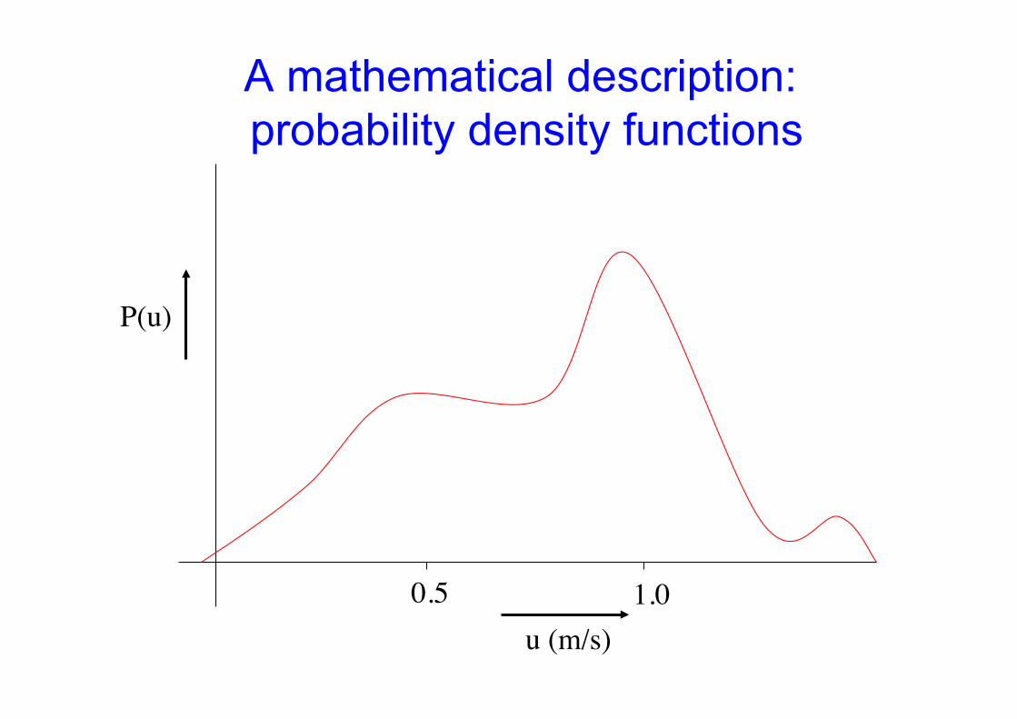
P(u)

u (m/s) 1.0 0.5

A mathematical description: probability density functions

Intermezzo: conditional pdf

Conditional pdf:

Similarly:

Combine:

Intermezzo: conditional pdf

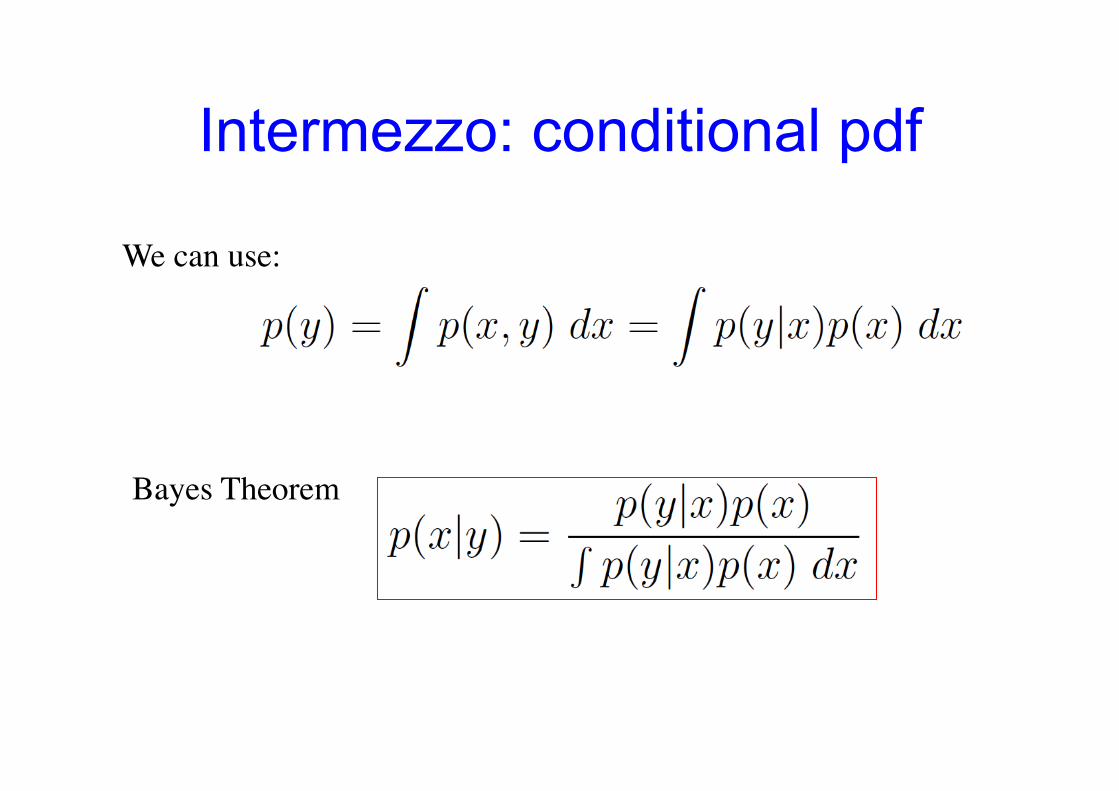
We can use:

Bayes Theorem

The model pdf p(x) p (u(x1), u(x2), T(x3), … )

u(x1)

u(x2)

T(x3)

Observations p(y|x)

•  In situ observations: irregular in space and

time e.g. sparse hydrographic observations,

•  Satellite observations: indirect

e.g. of the sea-surface

Thesolu)onisapdf!

Bayestheorem:

Data assimilation: general formulation

Filters and smoothers

Time

Filter: solve 3D problem sequentially

Smoother: solve 4D problem in specific time window all at once

Time

X

The Gaussian assumption

Prior pdf: multivariate Gaussian:

Likelihood: multivariate Gaussian

(Ensemble) Kalman Filter I

Use Gaussianity in Bayes at a specific time:

Multiplication:

Complete the squares to find again a Gaussian (only for linear H !!!):

(Ensemble) Kalman Filter III

Both lead to the Kalman filter equations, which are just the least squares solutions (best linear unbiased estimator, BLUE):

Two possibilities to find the expressions for the mean and covariance: 1)  Completing the squares 2)  Assume solution is linear combination of model and observations.

innovation weighting influence region K the Kalman Gain

Spatial correlation of SSH�and SST in the Indian Ocean

x

x

Haugen and Evensen, 2002

The error covariance:�

Tells us how model variables co-vary.

In the Kalman filter this comes in via the BHT term:

Kalman filters in practice: Ensembles How to propagate (or even store) the covariance matrix?

Ensemble Kalman Filter EnKF, ETKF, EAKF, …

Ensemble Kalman Filter: the update

Ensemble perturbation matrix

to represent prior covariance as:

Write posterior ensemble perturbations as:

Use to find

with

A variational method looks for the most probable state, which is the maximum of this posterior pdf also called the mode.

Instead of looking for the maximum one solves for the minimum of a so-called costfunction.

The pdf can be rewritten as

in which

Find min J from variational derivative: J is costfunction or penalty function

Variational methods

Gradient descent methods: Gauss-Newton iterations

J

model state xb

1 2 3 4 5 6 1’

4DVar There is an interesting extension to this formulation to a smoother.

Time

Filter: Solve a 3D problem at each observation time.

4DVar: Solve a 3D problem at the beginning of the time window using all observations. Note we get a new full 4D solution!

4DVar: the dynamical model

The dynamical model is denoted by M:

Using the model operator twice brings us to the next time step:

And some short-hand notation:

4DVar: the costfunction The total costfunction that we have to minimize now becomes:

in which the measurement operator Hi contains the forward model:

This nonlinear costfunction is minimised iteratively.

4DVar: the adjoint The solution to the linear iterates can be written as:

in which H now contains the model equations.

Note that HT contains the adjoint model equations, running from end of the time window to the initial time.

Present-day data-assimilation methods for NWP:

•  EnKF:

•  4DVar:

•  Hybrid methods: Combine the best of both. •  Nonlinear data-assimilation methods…

x

x

Nonlinear filtering: Particle filter

Use ensemble

with the weights.

What are these weights? •  The weight is the normalised value of the pdf of

the observations given model state . •  For Gaussian distributed variables is is given by:

•  One can just calculate this value •  That is all !!!

•  Or is it? More needed for high-dimensional problems…

Summary and outlook

•  We know how to formulate the data assimilation problem using Bayes Theorem. •  We have derived the Kalman Filter and shown that it is the best linear unbiased estimator (BLUE).

•  We derived 3D and 4DVar and discussed some of their properties.

•  We looked at a fully nonlinear method, the particle filter. •  This forms the basis for what is to come the rest of the

week!

ENJOY