Associated Legendre Polynomials andSpherical Harmonics Computation

for Chemistry Applications

Taweetham Limpanuparb ∗, Josh Milthorpe†

October 8, 2014

Abstract

Associated Legendre polynomials and spherical harmonics are central to calcula-tions in many fields of science and mathematics – not only chemistry but computergraphics, magnetic, seismology and geodesy. There are a number of algorithms forthese functions published since 1960 but none of them satisfy our requirements. Inthis paper, we present a comprehensive review of algorithms in the literature and,based on them, propose an efficient and accurate code for quantum chemistry. Ourrequirements are to efficiently calculate these functions for all non-negative integerdegrees and orders up to a given number (≤ 1000) and the absolute or the relativeerror of each calculated value should not exceed 10−10. We achieve this by nor-malizing the polynomials, employing efficient and stable recurrence relations, andprecomputing coefficients. The algorithm presented here is straightforward andmay be used in other areas of science.

1 Introduction

In 1782, Legendre1 introduced polynomials P` as the coefficients in the expansion of theNewtonian potential

1

r12=

1

|r1 − r2|=∞∑l=0

rl<rl+1>

P`(cos θ) (1)

where r< = min (|r1|, |r2|), r> = max (|r1|, |r2|) and r1 · r2 = |r1||r2| cos θ. AssociatedLegendre Polynomials (ALPs)a Pm

` of degree ` and order m ≥ 0 may be defined as themth derivative of P`,

Pm` (x) = (−1)m (1− x2)m/2 dm

dxmP`(x). (2)

∗Mahidol University International College, Mahidol University, Nakhonpathom 73170, Thailand Cor-responding author: taweetham.lim@mahidol.ac.th†IBM T.J. Watson Research Center, P.O. Box 704, Yorktown Heights, New York 10598, USAaALPs are sometimes referred to as Associated Legendre Functions (ALFs) because the (1− x2)m/2

factor is not a polynomial for odd m. This does not necessarily mean Associated Legendre functions ofthe second kind, Qµλ.

1

arX

iv:1

410.

1748

v1 [

phys

ics.

chem

-ph]

7 O

ct 2

014

The negative order can be related to the corresponding positive order via a proportionalityconstant that involves only ` and m,

P−m` (x) = (−1)m(`−m)!

(`+m)!Pm` (x). (3)

These ALPs are closely related to the spherical harmonics (SHs)b

Y m` (θ, φ) =

√(2`+ 1)(`−m)!

4π(`+m)!Pm` (cos θ) eimφ (4)

which are the analytic solutions for wavefunctions of the hydrogen atom and are commoningredients for some quantum chemistry calculations.2–10 It follows from the above equa-tions that Pm

` are the essential part for the computation of Y m` . In this manuscript, we

propose an algorithm to accurately and efficiently compute ALPs and SHs in the contextof quantum chemical applications. We note that the argument x = cos θ is real andbounded |x| ≤ 1 and both degree ` and order m are integers satisfying the conditions−` ≤ m ≤ ` and ` ≥ 0.

2 Review of algorithms for ALPs and SHs

The standard approach for special function calculation in quantum chemistry software isto use recurrence relations (RRs). However, there are a number of aspects that need tobe taken into consideration. There are myriad of RRs but not all of them are practical forcomputation using floating-point arithmetic. For some RRs, round-off error may rapidlypropagate and become significant if used in a certain direction. When the same RR isapplied in the reverse direction the numerical behavior might be the opposite. This isthe basis of Miller’s backward algorithm.11–14

Since the ultimate purpose of calculation is to obtain SHs, the ALPs may also bemodified or normalized to improve the stability of the RRs. ALPs and SHs have been asubject of numerous publications since 1960, but the best approach for ALP calculationmay differ depending on the application. “Numerical Recipes”, one of the most famousbooks on algorithms and numerical analysis, has even presented different algorithms inits second and third editions.15,16 The list below gives a brief summary of the algorithmsdeveloped over the past five decades ordered by year of publication. We indicate whetherPm` are normalized, however, normalization schemes differ between publications.

Ref Description

17 Calculation of P` by a RR in the direction of increasing `

18 Calculation of Pm` for ` < 20

Only half-page source code was provided in the manuscript.

19 Calculation of Pm` tested up to ` = m = 50

Start from P `` and use a RR in the direction of decreasing m.

bThere are several alternative definitions of ALPs and SHs which are commonly used in the fields ofmagnetic, geodesy and seismology. They are slightly different e.g. presence or absence of (−1)m or othernormalization factor. Our algorithm may be easily modified to suit their definitions.

2

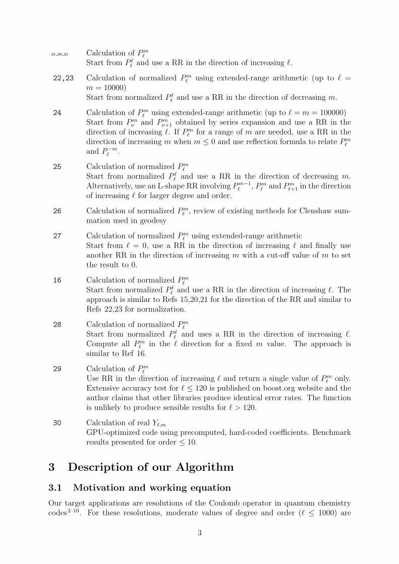
15,20,21 Calculation of Pm`

Start from P `` and use a RR in the direction of increasing `.

22,23 Calculation of normalized Pm` using extended-range arithmetic (up to ` =

m = 10000)Start from normalized P `

` and use a RR in the direction of decreasing m.

24 Calculation of Pm` using extended-range arithmetic (up to ` = m = 100000)

Start from Pmν and Pm

ν+1 obtained by series expansion and use a RR in thedirection of increasing `. If Pm

` for a range of m are needed, use a RR in thedirection of increasing m when m ≤ 0 and use reflection formula to relate Pm

`

and P−m` .

25 Calculation of normalized Pm`

Start from normalized P `` and use a RR in the direction of decreasing m.

Alternatively, use an L-shape RR involving Pm−1` , Pm

` and Pm`+1 in the direction

of increasing ` for larger degree and order.

26 Calculation of normalized Pm` , review of existing methods for Clenshaw sum-

mation used in geodesy

27 Calculation of normalized Pm` using extended-range arithmetic

Start from ` = 0, use a RR in the direction of increasing ` and finally useanother RR in the direction of increasing m with a cut-off value of m to setthe result to 0.

16 Calculation of normalized Pm`

Start from normalized P `` and use a RR in the direction of increasing `. The

approach is similar to Refs 15,20,21 for the direction of the RR and similar toRefs 22,23 for normalization.

28 Calculation of normalized Pm`

Start from normalized P `` and uses a RR in the direction of increasing `.

Compute all Pm` in the ` direction for a fixed m value. The approach is

similar to Ref 16.

29 Calculation of Pm`

Use RR in the direction of increasing ` and return a single value of Pm` only.

Extensive accuracy test for ` ≤ 120 is published on boost.org website and theauthor claims that other libraries produce identical error rates. The functionis unlikely to produce sensible results for ` > 120.

30 Calculation of real Y`,mGPU-optimized code using precomputed, hard-coded coefficients. Benchmarkresults presented for order ≤ 10.

3 Description of our Algorithm

3.1 Motivation and working equation

Our target applications are resolutions of the Coulomb operator in quantum chemistrycodes2–10. For these resolutions, moderate values of degree and order (` ≤ 1000) are

3

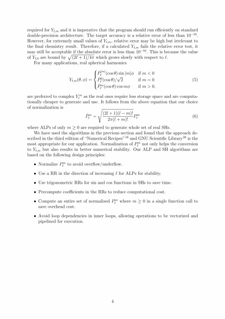
required for Y`,m and it is imperative that the program should run efficiently on standarddouble-precision architecture. The target accuracy is a relative error of less than 10−10.However, for extremely small values of Y`,m, relative error may be high but irrelevant tothe final chemistry result. Therefore, if a calculated Y`,m fails the relative error test, itmay still be acceptable if the absolute error is less than 10−10. This is because the valueof Y`,0 are bound by

√(2`+ 1)/4π which grows slowly with respect to `.

For many applications, real spherical harmonics

Y`,m(θ, φ) =

P|m|` (cos θ) sin |m|φ if m < 0

P 0` (cos θ)/

√2 if m = 0

Pm` (cos θ) cosmφ if m > 0.

(5)

are preferred to complex Y m` as the real ones require less storage space and are computa-

tionally cheaper to generate and use. It follows from the above equation that our choiceof normalization is

Pm` =

√(2l + 1)(l −m)!

2π(l +m)!Pm` (6)

where ALPs of only m ≥ 0 are required to generate whole set of real SHs.We have used the algorithms in the previous section and found that the approach de-

scribed in the third edition of “Numerical Recipes”16 and GNU Scientific Library28 is themost appropriate for our application. Normalization of Pm

` not only helps the conversionto Y`,m but also results in better numerical stability. Our ALP and SH algorithms arebased on the following design principles:

• Normalize Pm` to avoid overflow/underflow.

• Use a RR in the direction of increasing ` for ALPs for stability.

• Use trigonometric RRs for sin and cos functions in SHs to save time.

• Precompute coefficients in the RRs to reduce computational cost.

• Compute an entire set of normalized Pm` where m ≥ 0 in a single function call to

save overhead cost.

• Avoid loop dependencies in inner loops, allowing operations to be vectorized andpipelined for execution.

4

The set of working equations for our algorithm is described below.

am` =

√4l2 − 1

l2 −m2(7)

bm` = −

√(l − 1)2 −m2

4(l − 1)2 − 1(8)

P 00 =

√1

2π(9)

x = cos θ (10)

y = sin θ (11)

Pmm = −

√1 +

1

2my Pm−1

m−1 (12)

Pmm+1 =

√2m+ 3 xPm

m (13)

Pm` = am` (xPm

`−1 + bm` Pm`−2) (14)

To reduce the computational cost, two-term RRs

cosmφ = 2 cosφ cos(m− 1)φ− cos(m− 2)φ (15)

sinmφ = 2 cosφ sin(m− 1)φ− sin(m− 2)φ (16)

or one-term RRs

cos(mφ) = cosψ − [α cosψ + β sinψ] (17)

sin(mφ) = sinψ − [α sinψ − β cosψ] (18)

α = 2 sin2

(φ

2

)(19)

β = sinφ (20)

ψ = (m− 1)φ (21)

may also be used to calculate the sinusoidal functions in SHs. Using the RRs, sinφ andcosφ are the only two expensive transcendental function operations required to generatethe whole set of SHs.

3.2 Implementation

Initialization

The coefficients am` (7) and bm` (8) are precomputed for all ` ≤ L,m ≤ ` as follows:

1 #define PT(l,m) ((m)+((l)*((l)+1))/2)

23 for (size_t l=2; l<=LL; l++) {

4 double ls=l*l, lm1s = (l-1)*(l-1);

5 for (size_t m=0; m<l-1; m++) {

6 double ms=m*m;

7 A[PT(l,m)] = sqrt ((4*ls -1.)/(ls-ms));

8 B[PT(l,m)] = -sqrt((lm1s -ms)/(4*lm1s -1.));

9 }

10 }

5

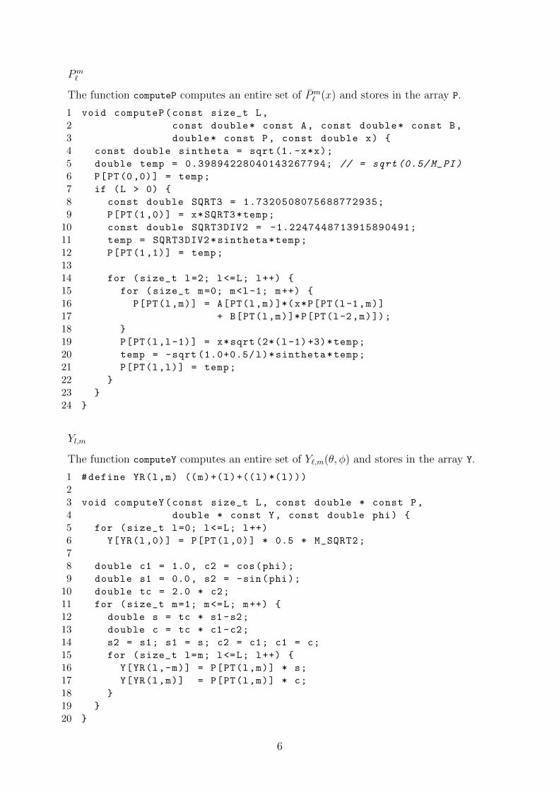
Pm`

The function computeP computes an entire set of Pm` (x) and stores in the array P.

1 void computeP(const size_t L,

2 const double* const A, const double* const B,

3 double* const P, const double x) {

4 const double sintheta = sqrt(1.-x*x);

5 double temp = 0.39894228040143267794; // = sqrt (0.5/ M_PI)

6 P[PT(0,0)] = temp;

7 if (L > 0) {

8 const double SQRT3 = 1.7320508075688772935;

9 P[PT(1,0)] = x*SQRT3*temp;

10 const double SQRT3DIV2 = -1.2247448713915890491;

11 temp = SQRT3DIV2*sintheta*temp;

12 P[PT(1,1)] = temp;

1314 for (size_t l=2; l<=L; l++) {

15 for (size_t m=0; m<l-1; m++) {

16 P[PT(l,m)] = A[PT(l,m)]*(x*P[PT(l-1,m)]

17 + B[PT(l,m)]*P[PT(l-2,m)]);

18 }

19 P[PT(l,l-1)] = x*sqrt (2*(l-1)+3)*temp;

20 temp = -sqrt (1.0+0.5/l)*sintheta*temp;

21 P[PT(l,l)] = temp;

22 }

23 }

24 }

Yl,m

The function computeY computes an entire set of Y`,m(θ, φ) and stores in the array Y.

1 #define YR(l,m) ((m)+(l)+((l)*(l)))

23 void computeY(const size_t L, const double * const P,

4 double * const Y, const double phi) {

5 for (size_t l=0; l<=L; l++)

6 Y[YR(l,0)] = P[PT(l,0)] * 0.5 * M_SQRT2;

78 double c1 = 1.0, c2 = cos(phi);

9 double s1 = 0.0, s2 = -sin(phi);

10 double tc = 2.0 * c2;

11 for (size_t m=1; m<=L; m++) {

12 double s = tc * s1 -s2;

13 double c = tc * c1 -c2;

14 s2 = s1; s1 = s; c2 = c1; c1 = c;

15 for (size_t l=m; l<=L; l++) {

16 Y[YR(l,-m)] = P[PT(l,m)] * s;

17 Y[YR(l,m)] = P[PT(l,m)] * c;

18 }

19 }

20 }

6

4 Numerical results

4.1 Accuracy

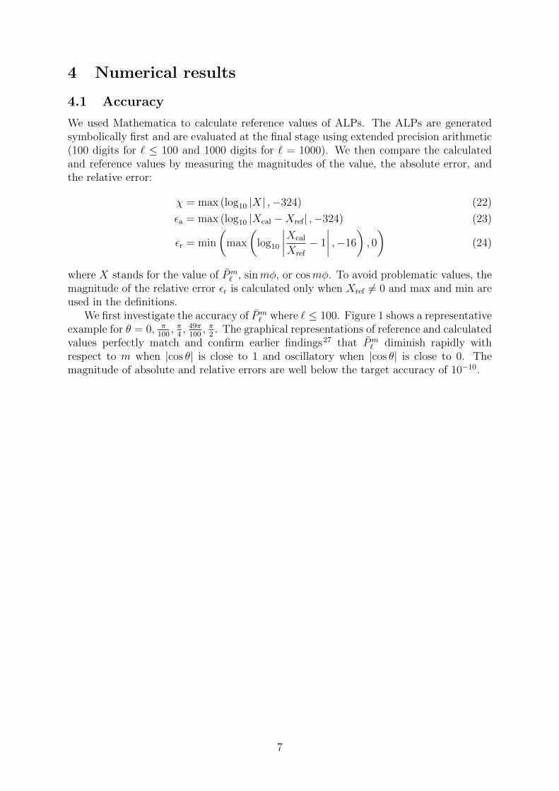
We used Mathematica to calculate reference values of ALPs. The ALPs are generatedsymbolically first and are evaluated at the final stage using extended precision arithmetic(100 digits for ` ≤ 100 and 1000 digits for ` = 1000). We then compare the calculatedand reference values by measuring the magnitudes of the value, the absolute error, andthe relative error:

χ = max (log10 |X| ,−324) (22)

εa = max (log10 |Xcal −Xref| ,−324) (23)

εr = min

(max

(log10

∣∣∣∣Xcal

Xref

− 1

∣∣∣∣ ,−16

), 0

)(24)

where X stands for the value of Pm` , sinmφ, or cosmφ. To avoid problematic values, the

magnitude of the relative error εr is calculated only when Xref 6= 0 and max and min areused in the definitions.

We first investigate the accuracy of Pm` where ` ≤ 100. Figure 1 shows a representative

example for θ = 0, π100, π4, 49π100, π2. The graphical representations of reference and calculated

values perfectly match and confirm earlier findings27 that Pm` diminish rapidly with

respect to m when |cos θ| is close to 1 and oscillatory when |cos θ| is close to 0. Themagnitude of absolute and relative errors are well below the target accuracy of 10−10.

7

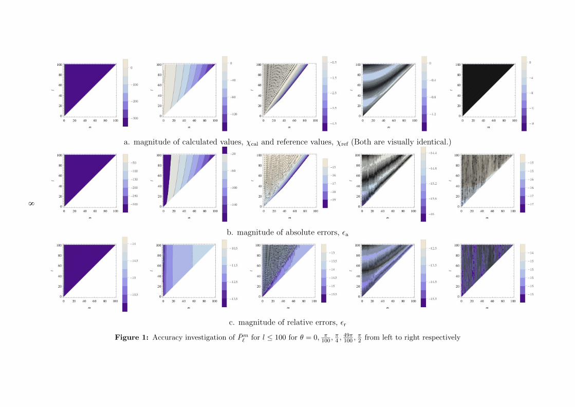
a. magnitude of calculated values, χcal and reference values, χref (Both are visually identical.)

b. magnitude of absolute errors, εa

c. magnitude of relative errors, εr

Figure 1: Accuracy investigation of Pm` for l ≤ 100 for θ = 0, π100 ,

π4 ,

49π100 ,

π2 from left to right respectively

8

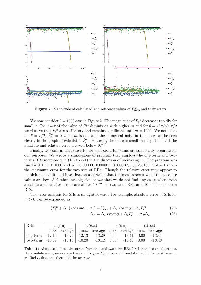
Figure 2: Magnitude of calculated and reference values of Pm1000 and their errors

We now consider ` = 1000 case in Figure 2. The magnitude of Pm` decreases rapidly for

small θ. For θ = π/4 the value of Pm` diminishes with higher m and for θ = 49π/50, π/2

we observe that Pm` are oscillatory and remains significant until m = 1000. We note that

for θ = π/2, Pm` = 0 when m is odd and the numerical noise in this case can be seen

clearly in the graph of calculated Pm` . However, the noise is small in magnitude and the

absolute and relative error are well below 10−10.Finally, we confirm that the RRs for sinusoidal functions are sufficiently accurate for

our purpose. We wrote a stand-alone C program that employs the one-term and two-terms RRs mentioned in (15) to (21) in the direction of increasing m. The program wasrun for 0 ≤ m ≤ 1000 and φ = 0.000000, 0.000001, 0.000002, ..., 6.283185. Table 1 showsthe maximum error for the two sets of RRs. Though the relative error may appear tobe high, our additional investigation ascertains that those cases occur when the absolutevalues are low. A further investigation shows that we do not find any cases where bothabsolute and relative errors are above 10−10 for two-term RRs and 10−12 for one-termRRs.

The error analysis for SHs is straightforward. For example, absolute error of SHs form > 0 can be expanded as(

Pm` + ∆P

)(cosmφ+ ∆c) = Y`,m + ∆P cosmφ+ ∆cP

m` (25)

∆Y = ∆P cosmφ+ ∆cPm` + ∆P∆c. (26)

RRs εa(sin) εa(cos) εr(sin) εr(cos)max average max average max average max average

one-term -12.13 -13.29 -12.13 -13.29 0.00 -13.41 0.00 -13.41two-term -10.59 -13.16 -10.20 -13.12 0.00 -13.43 0.00 -13.43

Table 1: Absolute and relative errors from one- and two-term RRs for sine and cosine functions.For absolute error, we average the term |Xcal −Xref| first and then take log but for relative errorwe find εr first and then find the average.

9

It is obvious that the last term ∆P∆c is negligible and the behavior of the other twoerror terms are more or less predictable since ∆ is multiplied to a bounded function. The

largest Pm` in our case is P 0

1000(1) =√

20012π≈ 18. Since absolute errors, ∆P and ∆c are

well below 10−10 we conclude that the resulting ∆Y is also below this threshold providedthat one-term RRs are used for the trigonometry functions. A similar analysis is alsoapplicable to m = 0 (change cosmφ, ∆c to 1/

√2, 0) and m < 0 (change cosmφ, ∆c to

sinmφ, ∆s).From the analysis here, it is anticipated that our algorithm may be used beyond

` = 1000. However, trigonometric RRs may be less attractive as the computational costsaving is no longer significant. A cut-off scheme for small values may be more helpfulin this circumstance. We do not provide an analysis for this as the reference values aredifficult to calculate and it is beyond the scope of our chemical applications.

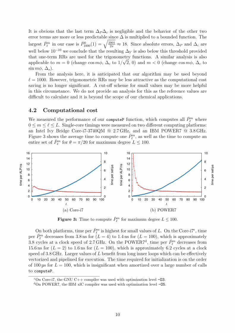
4.2 Computational cost

We measured the performance of our computeP function, which computes all Pm` where

0 ≤ m ≤ ` ≤ L. Single-core timings were measured on two different computing platforms:an Intel Ivy Bridge Core-i7-3740QM @ 2.7 GHz, and an IBM POWER7 @ 3.8 GHz.Figure 3 shows the average time to compute one Pm

` , as well as the time to compute anentire set of Pm

` for θ = π/20 for maximum degree L ≤ 100.

0

2

4

6

8

10

12

14

16

0 10 20 30 40 50 60 70 80 90 100 0

2

4

6

8

10

tim

e p

er

AL

P/n

s

tim

e p

er

se

t/µ

s

L

(a) Core-i7

0

2

4

6

8

10

12

14

16

0 10 20 30 40 50 60 70 80 90 100 0

2

4

6

8

10

tim

e p

er

AL

P/n

s

tim

e p

er

se

t/µ

s

L

(b) POWER7

Figure 3: Time to compute Pm` for maximum degree L ≤ 100.

On both platforms, time per Pm` is highest for small values of L. On the Core-i7c, time

per Pm` decreases from 3.8 ns for (L = 4) to 1.4 ns for (L = 100), which is approximately

3.8 cycles at a clock speed of 2.7 GHz. On the POWER7d, time per Pm` decreases from

15.6 ns for (L = 2) to 1.6 ns for (L = 100), which is approximately 6.2 cycles at a clockspeed of 3.8 GHz. Larger values of L benefit from long inner loops which can be effectivelyvectorized and pipelined for execution. The time required for initialization is on the orderof 100 µs for L = 100, which is insignificant when amortized over a large number of callsto computeP.

cOn Core-i7, the GNU C++ compiler was used with optimization level -O3.dOn POWER7, the IBM xlC compiler was used with optimization level -O5.

10

5 Concluding remarks

We have proposed an algorithm for the calculation of ALPs and SHs. Accuracy analysiswas conducted for degree and order up to 1000 and found that absolute or relative errorare satisfactorily below 10−10. Timing experiments showed that our C++ implementationtakes less than four cycles on average to produce an ALP. This new code will be used inour future quantum chemistry work.

References

[1] A.-M. Legendre, Memoires de Mathematiques et de Physique, presentes a l’Academie royaledes sciences (Paris), 1785, 10, 411–435.

[2] S. A. Varganov, A. T. B. Gilbert, E. Deplazes and P. M. W. Gill, J. Chem. Phys., 2008,128, 201104.

[3] P. M. W. Gill and A. T. B. Gilbert, Chem. Phys., 2009, 356, 86–90.

[4] T. Limpanuparb and P. M. W. Gill, Phys. Chem. Chem. Phys., 2009, 11, 9176–9181.

[5] T. Limpanuparb, A. T. B. Gilbert and P. M. W. Gill, J. Chem. Theory Comput., 2011, 7,830–833.

[6] T. Limpanuparb and P. M. W. Gill, J. Chem. Theory Comput., 2011, 7, 2353–2357.

[7] T. Limpanuparb, J. W. Hollett and P. M. W. Gill, J. Chem. Phys., 2012, 136, 104102.

[8] T. Limpanuparb, J. Milthorpe, A. Rendell and P. Gill, J. Chem. Theory Comput., 2013,9, 863–867.

[9] T. Limpanuparb, J. Milthorpe and A. Rendell, J. Comput. Chem., 2014, 35, In press.

[10] T. Limpanuparb, Applications of Resolutions of the Coulomb Operator in Quantum Chem-istry, PhD dissertation, Australian National University, http://hdl.handle.net/1885/8879,2012.

[11] W. Gautschi, SIAM Rev., 1967, 9, 24–82.

[12] F. W. J. Olver and D. J. Sookne, Math. Comput., 1972, 26, 941–947.

[13] F. W. J. Olver, Math. Comput., 1964, 18, 65–74.

[14] Lord Rayleigh (J. W. Strutt), Proc. R. Soc. A, 1910, 84, 25–46.

[15] W. H. Press, S. A. Teukolsky, W. T. Vetterling and B. P. Flannery, Numerical Recipes inC. The art of scientific computing, Cambridge University Press, 2nd edn., 1992, vol. 1.

[16] W. H. Press, Numerical Recipes 3rd edition: The art of scientific computing, CambridgeUniversity Press, 2007.

[17] G. Galler, Commun. ACM, 1960, 3, 353.

[18] J. R. Herndon, Commun. ACM, 1961, 4, 178–179.

[19] R. A. Wiggins and M. Saito, Bull. Seismol. Soc. Am., 1971, 61, 375–381.

11

[20] W. Braithwaite, Comput. Phys. Commun., 1973, 5, 390–394.

[21] B. I. Schneider, J. Segura, A. Gil, X. Guan and K. Bartschat, Comput. Phys. Commun.,2010, 181, 2091–2097.

[22] J. Smith, F. Olver and D. W. Lozier, ACM T. Math. Software, 1981, 7, 93–105.

[23] D. W. Lozier and J. Smith, ACM T. Math. Software, 1981, 7, 141–146.

[24] F. Olver and J. Smith, J. Comput. Phys., 1983, 51, 502–518.

[25] K. G. Libbrecht, Sol. Phys., 1985, 99, 371–373.

[26] S. A. Holmes and W. E. Featherstone, J. Geodesy, 2002, 76, 279–299.

[27] C. Jekeli, J. K. Lee and J. H. Kwon, J. Geodesy, 2007, 81, 603–615.

[28] M. Galassi, J. Davies, J. Theiler, B. Gough, G. Jungman, P. Alken, M. Booth and F. Rossi,GNU scientific library reference manual, Network Theory Ltd., 2009.

[29] B. Schling, The Boost C++ libraries, XML Press, 2011.

[30] P.-P. Sloan, J. Comput. Graph. Techniques, 2013, 2, 84–90.

12